a nano-scale multi-asperity contact and friction...
TRANSCRIPT
1
A Nano-Scale Multi-Asperity Contact and Friction Model
George G. Adams, Sinan Müftü and Nazif Mohd Azhar
Department of Mechanical, Industrial and Manufacturing Engineering, 334 SN
Northeastern University
Boston, MA 02115, USA
Submitted to Journal of Tribology, ASME Transactions, for review
September 2002
AbstractAs surfaces become smoother and loading forces decrease in applications such as MEMS andNEMS devices, the asperity contacts which comprise the real contact area will continue todecrease into the nano scale regime. Thus it becomes important to understand how the materialand topographical properties of surfaces contribute to measured friction forces at this nano scale.
In this investigation, the single asperity nano contact model of Hurtado and Kim isincorporated into a multi-asperity model for contact and friction which includes the effect ofasperity adhesion forces using the Maugis-Dugdale model. The model spans the range fromnano-scale to micro-scale to macro-scale contacts. Three key dimensionless parameters havebeen identified which represent combinations of surface roughness measures, Burgers vectorlength, surface energy, and elastic properties. Results are given for the friction coefficient vs.normal force, the normal and friction forces vs. separation, and the pull-off force for variousvalues of these key parameters.
Keywords: friction coefficient; contact; nanocontacts; multi-asperity models.

2
NomenclatureA = real contact area
AM = Maugis model contact radiusA = contact radius correction factor
B = y-intercept of region-2 of HKE = Young’s modulus
E* = composite Young’s modulusF = friction forceFf = friction force on a single asperity
F = dimensionless shear forceG = shear modulus
G* = effective shear modulusK = plane stress correction factor
M = slope of curve in region-2 of HKN = number of asperitiesP = normal forceP = dimensionless normal force
PM = Maugis model normal forceP = normal force correction factorR = radius of asperity curvaturea = contact radius
a = dimensionless contact radiusb = Burgers vector magnitudec = adhesion contact radiusd = separation
d = dimensionless separationh = maximum adhesion distancek = scaling factor
m = ratio of the radii of the adhesion region to the Hertz contact regionu = normal approach
u = dimensionless normal approachw = surface energy of adhesionz = asperity heightz = dimensionless asperity heights
α = surface roughness parameterβ = friction regime parameterγ = surface energy/compliance coefficient
δ = normal approach correction factor∆M = Maugis model penetration
λ = dimensionless adhesion parameterµ = static coefficient of frictionν = Poisson’s ratioσ = standard deviation of asperity peak heights
σo = adhesive tensile stressτf = friction stress
1 2,f fτ τ = shear stress at upper and lower limits of the HK model
φ = asperity peak probability distribution
3
IntroductionContact and friction affect the operation of many machines and tools we use every day, as wellas some of the most basic activities in nature. Examples range from belt drives, brakes, tires,clutches, in automobiles and in other machines; gears, bearings and seals in a variety ofmechanical systems; electrical contacts in motors; slider-disk interactions in a disk drive; MEMSmotors; a robotic manipulator joint; the motion of a human knee-joint (natural or artificial); andwalking/running on the ground. From these examples it is clear that friction can be beneficial(e.g. brakes, tires, walking) or detrimental (e.g. bearings, seals, robotic or human joints).Friction can also be classified as dynamic (e.g. sliding contact in brakes, slider-disk interactions,motion of joints) or predominately static (i.e. little, if any, relative motion, which may includemicro-slip as in rolling of train wheels, belt drives, and walking). Friction may also be classifiedas dry (i.e. without an intervening lubricant as with brakes, tires, and walking) or lubricated (e.g.slider-disk interactions, bearings, and human joints).
The friction force F is the tangential force resisting the relative motion of two surfaceswhich are pressed against each other with a normal force P. Amontons, in 1699, and Coulomb in1785, developed our phenomenological understanding of dry friction between two contactingbodies. Amontons-Coulomb friction states that the ratio of the friction force (during sliding) tothe normal force acting is a constant called the coefficient of kinetic friction. Similarly thecoefficient of static friction is the ratio of the maximum friction force that the surfaces cansustain, without relative motion, to the normal force. Experiments show that static friction issomewhat greater than dynamic friction. We can summarize these friction laws by defining thecoefficient of friction µ as
F
Pµ = (1)
without distinguishing between static and low-speed sliding friction. Although Eq. (1) providesan extraordinarily simple phenomenological friction law, the nature of the friction force is not atall well-understood.
Tabor [1] reviewed the state of understanding of friction phenomenon as it existed twodecades ago. Friction was originally thought to be due to the resistance of asperities on onesurface riding over the asperities of the mating surface. The distinction between static anddynamic friction was attributed to the asperities jumping over the gap between neighboringasperities on the other surface during sliding. The main criticism of this roughness theory offriction is that it is a conservative process whereas friction is known to be dissipative.Nonetheless the terminology of “smooth” and “rough” to represent frictionless and frictionalcontact respectively still persists in, for example, many elementary mechanics textbooks.
The adhesion theory of friction relates roughness to friction in a different manner [1].Because real surfaces always possess some degree of roughness (Fig. 1), the contact between twobodies occurs at or near the peaks of these contacting asperities. Thus the real area of contactwill generally be much less than the apparent contact area and the average normal stress in thereal contact area can easily exceed the material hardness. If each asperity contact is viewed as aplastic indentation, then the normal contact stress is constant, and the real area of contact isproportional to the normal force. Thus the adhesion theory of friction, which gives a frictionforce proportional to the real contact area, also gives the required proportionality between thefriction force and the normal load for Amontons-Coulomb friction, i.e. Eq. (1). However even inthe absence of plastic deformation, the real area of contact is nearly proportional to the normalload if the asperities have a statistical distribution of heights (Geeenwood and Williamson, [2]).Thus Tabor [1] lists the following three basic elements contributing to the friction ofunlubricated solids: (1) the real contact area between the sliding surfaces; (2) the type and the
4
strength of the bond at the contact interface; and (3) the shearing and rupturing characteristics ofthe material in and around the contact regions. These basic elements can be strongly affected byvarious factors such as the presence of oxide films, the contact size of individual asperities, andtemperature effects.
Consequently, contact modeling becomes an essential part of any friction model. Itconsists of two related steps. First, the equations representing the contact of a single pair ofasperities are determined. In general this procedure includes elastic, elastic-plastic, orcompletely plastic deformation. Depending on the scale of the contact, plasticity effects may bepenetration-depth dependent (Hutchinson, [3]). For nanometer scale contacts the effect ofadhesion on the contact area is important. Second, the cumulative effects of individual asperitiesare determined. Conventional multi-asperity contact models may be categorized aspredominately uncoupled or predominately coupled. Uncoupled contact models representsurface roughness as a set of asperities, often with statistically distributed parameters. The effectof each individual asperity is local and considered separately from the other asperities; thecumulative effect is the summation of the actions of individual asperities. Coupled modelsinclude the effect of the loading on one asperity on the deformation of neighboring asperities.Such models are far more complex mathematically than the uncoupled models and for thatreason have been used less frequently.
The well-known solution for the single contact area between two elastic bodies wasdeveloped in the late nineteenth century by Hertz. The assumptions for what has become knownas the Hertz contact problem are: (1) the contact area is elliptical; (2) each body is approximatedby an elastic half-space loaded over an elliptical contact area; (3) the dimensions of the contactarea must be small compared to the dimensions of each body and to the radii of curvature of thesurfaces; (4) the strains are sufficiently small for linear elasticity to be valid; and (5) the contactis frictionless, so that only a normal pressure is transmitted. For the case of solids of revolution,the contact area is circular. The interference, contact radius, and maximum contact pressure aregiven by simple equations [4] which depend upon the Young’s moduli, the Poisson’s ratios, theradii of curvature, and the applied force.
Various statistical models of multi-asperity contact have been developed in order todetermine the normal contact force, many of which are related in some way to the pioneeringwork of Greenwood and Williamson (GW) [2]. The GW model assumes that in the contactbetween one rough and one smooth surface: (1) the rough surface is isotropic; (2) asperities arespherical near their summits; (3) all asperity summits have the same radius of curvature whiletheir heights vary randomly; (4) there is no interaction between neighboring asperities; and (5)there is no bulk deformation. The first three assumptions were relaxed by McCool [5] whotreated anisotropic rough surfaces with ellipsoidal asperities. However his results were in goodagreement with the simpler GW model. Greenwood and Tripp [6] showed that the contact oftwo rough surfaces can be replaced with the contact of a single rough body with a smoothsurface.
For sufficiently small size contacts, the normal adhesion forces between the surfacesaffect the contact conditions. Various adhesion models, between an elastic sphere and a flat,have been introduced. The model by Johnson, Kendall and Roberts (JKR) assumes that theattractive intermolecular surface forces cause elastic deformation beyond that predicted by theHertz theory, and produces a subsequent increase of the contact area [7]. This model alsoassumes that the attractive forces are confined to the contact area and are zero outside the contactarea. The model by Derjaguin, Muller and Toporov (DMT), on the other hand, assumes that thecontact area does not change due to the attractive surface forces and remains the same as in theHertz theory [8]. In this model the attractive forces are assumed to act only outside of thecontact area. Due to the assumptions involved, the JKR model is more suitable for soft materials

5
and the DMT model is more appropriate for harder materials. Another model, introduced byMaugis [9], describes a continuous transition between the JKR and DMT models [10]. In orderto represent the surface forces, Maugis used a Dugdale approximation [11] in which theattractive stress is a constant 0σ for surface separations up to a prescribed value h. Intimate
contact is maintained over a central region of radius 0 r a≤ ≤ , an adhesive stress of constantmagnitude 0σ acts outside the contact zone in a r c≤ ≤ , and the region cr > is stress-free.
Models to predict the friction force in a multi-asperity contact are relatively few. In thefirst of a series of papers Chang, Etsion and Bogy (CEB) [12] developed an elastic-plastic multi-asperity contact model for normal loading based on volume conservation of a plasticallydeformed asperity control volume. In [13], the effect of adhesion was included in the multi-asperity contact model of [12] by using the DMT model for contacting asperities and theLennard-Jones potential between non-contacting asperities. The DMT model was used becauseit was thought to be appropriate for the contact of hard metal surfaces. The effects of the surfaceenergy of adhesion and of the surface roughness, on the adhesion force and on the pull-off forcewere examined. Finally a model for calculating the coefficient of friction was given in [14]. Itassumed that once plastic yielding is initiated in a pair of contacting asperities, no furthertangential force can be sustained. In order to calculate this limiting shear force, the stress fieldfor an asperity subject to normal and lateral tractions developed by Hamilton [15] was used. Fora given normal load, the maximum tangential force that can be sustained before the initiation ofplastic yielding (based upon the von Mises yield criterion) was calculated. Thus any asperitywhich was plastically deformed under normal loading cannot resist a lateral load. Chang, Etsionand Bogy then calculated the total shear force that a multi-asperity interface can sustain byintegrating the shear force relation statistically as in the GW model. They showed that the staticcoefficient of friction decreases with increasing plasticity index and that it increases withincreasing surface energy. Also as the external normal force increases, the static frictioncoefficient decreases. This latter result is contrary to ordinary Amonton-Coulomb friction, butconsistent with the results of various experimental investigations cited in [14].
Fuller and Tabor [16] investigated the effect of roughness on the adhesion betweenelastic bodies. Experiments were conducted between rubber spheres and a hard flat surface withcontrolled roughness. A theoretical model which used the JKR model of adhesion along with aGaussian distribution of asperity heights was developed. Their work showed that relativelysmall surface roughness is sufficient to reduce the adhesion between the surfaces to a very smallvalue. A key parameter was identified which depends on surface energy, composite elasticmodulus, standard deviation of asperity heights, and asperity curvature.
Stanley, Etsion and Bogy (SEB) [17] developed a model for the adhesion of two roughsurfaces, affected by sub-boundary layer lubrication, in elastic-plastic multi-asperity contact.Sub-boundary lubrication occurs when an extremely thin layer of lubricant is applied to a solidsurface and forms a strong bond with the surface, without tending to form menisci. The analysisin [17] showed that even though the introduction of the lubricant reduces the surface free energy,there can be an increase in the overall adhesive force relative to the dry case without theformation of liquid meniscus bridges. A roughness-dependent critical lubricant thickness exists,above which the adhesion force increases rapidly. Polycarpou and Etsion [18] used the SEBmodel to predict the static friction coefficient in the presence of sub-boundary layer lubrication.The tangential load was found using the same procedure as in the CEB model [14] for solid-solidcontact. They found that the coefficient of friction increases with decreasing normal load andthat a roughness-dependent critical lubricant thickness exists, above which the adhesion forceincreases rapidly within the sub-boundary regime.
6
One of the interesting and important results of the GW model is that the real area ofcontact is roughly proportional to the normal load. Thus if the friction stress is constant, thefriction force is proportional to the real area of contact, and hence the friction force will beroughly proportional to the normal load. This leads to a coefficient of friction which is nearlyindependent of normal load. However recent experimental evidence shows that there is asignificant change in the friction stress τf acting on a single asperity contact, as the contact areachanges from the micro to nano scale. Experiments, in which the friction force is measuredusing an atomic force microscope (AFM) [19], show that the friction stress can be more than anorder of magnitude higher as compared to experiments in which the friction is measured with thesurface force apparatus (SFA) [20]. A typical contact radius for an AFM tip is estimated to beon the order of 3-14 nm, whereas for SFA it is on the order of 40-250 µm.
The scale dependence of the friction stress has recently been investigated by Hurtado andKim (HK), [21,22]. They presented a micromechanical dislocation model of frictional slipbetween two asperities for a wide range of contact radii. According to the HK model, if thecontact radius a is smaller than a critical value, the asperities slide past each other in a concurrentslip process, where the adhesive forces are responsible for the shear stress; hence the shear stressremains at a high constant value. On the other hand, if the contact radius is greater than thecritical value, the shear stress decreases for increasing values of contact radius until it reaches asecond constant, but lower value. This behavior is approximated in Fig. 2. In the transitionregion between the two critical contact radius values, single dislocation assisted slip takes place,where a dislocation loop starts in periphery of the contact region and grows toward the center;the shear stress is dominated by the resistance of the dislocation to motion. Multi-dislocation-cooperated slip is responsible for the friction stress in the second constant shear stress region[21]. It is emphasized that in the HK model the dislocation motion is confined to the interface;hence bulk plastic deformation need not occur.
The HK model provides an expression for the behavior of the friction stress over a widerange of contact areas, including nano scale contacts. In this paper, as in the Adams, Müftü, andMohd Azhar (AMM) model [23], the frictional slip model of Hurtado and Kim, and the adhesioncontact model of Maugis, are combined with the Greenwood and Williamson statistical multi-asperity contact model, in order to derive the relationship between the friction force F and thenormal load P between two rough surfaces during a slip process. The attractive forces betweenasperities that are not in contact are neglected. The coefficient of friction µ is then calculated asthe ratio of the shear force to the applied normal load. Three dimensionless parameters thatrepresent the surface roughness, the friction regime of the contacts, and the surfaceenergy/compliance, are seen to influence the value of the friction coefficient. The effect ofvarying these three parameters on the coefficient of friction and on the pull-off force isdiscussed.
Development of the ModelHurtado-Kim ModelHurtado and Kim (HK) [21,22] presented a micromechanical dislocation model of frictional slipbetween two asperities which states that, for contact radii smaller than a critical value, thefriction stress is constant. Above that critical value, the friction stress decreases as the contactradius increases until a second transition occurs where the friction stress again becomesindependent of the contact size. The relationship between the non-dimensional friction stress
f f Gτ τ= / * and the non-dimensional contact radius /a a b= , according to Hurtado and Kim is
given in Fig. 2. The contact radius a is normalized by the Burgers vector b and the friction stress

7
fτ is normalized by the effective shear modulus G*=2G1G2/(G1+G2) where G1 and G2 are the
shear moduli of the contacting bodies. In this figure, region-1 represents typical experimentalvalues obtained using the atomic force microscope (AFM) while region-3 represents the typicalexperimental values obtained with the surface force apparatus (SFA). These two regions areconnected by the transition region-2.
From Fig. 2, the dimensionless shear stress is a function of the dimensionless contactradius and can be approximated by
( )1
2
1
1 2
2
f
f
f
a a
M a B a a a
a a
ττ
τ
<
= + < < >
log ,
log log ,
log , (2)
where the left and right limits of region-2 are ( )11, fa τ and ( )
22, fa τ respectively. The constants
of Eq. (2) are given by
( )( ) ( )( )( ) ( ) ( ) ( )( ) ( )( )
1 2
1 2
2 1
2 1 2 1
f f
f f
M a a
B a a a a
τ τ
τ τ
= −
= −
log log
log log log log log
(3)
The friction force Ff acting on a single asperity can be determined from Eq. (2) by using the
relationship 2f fF aπ τ= as follows
1
2
21
21 22
22
10
f
f B M
f
a a aF
a a a aG b
a a a
τ
τ
+
<
= < < >
,
,*
,
(4)
A Multi-Asperity Friction Model Based on the HK ModelThe maximum shear force in the static contact of two asperities can be predicted by the HKmodel given in Eq. (4). The Greenwood and Williamson model describes the multi-asperitycontact of two real rough surfaces [2]. The conditions for which the GW model are valid, givenin the Introduction, are assumed to hold here. Then, when two real surfaces are separated by adistance d the number of contacting asperities n can be found from
( )d
n N z dzφ∞
= ∫ (5)
where N is the total number of asperities, σ is the standard deviation of asperity peak heights,
z z σ= is the dimensionless height coordinate measured from the mean of asperity heights,
( )zφ is the probability density of asperity peaks, and d d σ= is the non-dimensional
separation between the two surfaces. The general relation between the normal load P and thedeformation u of two spherical asperities in contact is given by the Hertz contact theory as
( ) 1 2 3 24 3 * / /P E R u= , where R is the composite radius of curvature of the asperity tips, and *E is
the composite Young’s modulus of the two materials [4]. In this work, one of the surfaces isassumed to be rigid and flat. Thus the composite Young’s modulus is given by 21E E ν= −* ( ) andG*=2G where ν, E, G are the Poisson’s ratio, Young’s modulus, and shear modulus of the elasticbody respectively. The total deformation u of the asperities is equal to the penetration, i.e.u z d= − , as shown in Fig. 1.

8
Thus the GW model gives the non-dimensional normal force per asperity P between twonominally flat, otherwise rough surfaces, separated by a distance d as
( ) ( )3 222
4 2
3 1 d
PP z d z dz
NGbαβ φ
ν
∞
= = −− ∫
/ (6)
In Eq. (6), the two non-dimensional surface parameters α and β have been defined as1 2/
R
σα = , ( )1 2/
R
b
σβ = , (7)
and the relation G=E/2(1+ν) has been used. For Hertz contact, the dimensionless relations for asingle asperity contact are
( )1 2
1 2Rua z d
bβ= = −
//( ) or
2
2
az d
β= + . (8)
In order to provide a physical interpretation of the surface parameters α and β, it is notedthat in a simple vertical scaling of the surface by a factor k, the standard deviation of asperityheights σ is scaled by k but the asperity radius of curvature R is scaled by 1/k. Thus, α is scaledby k, but β remains constant. Hence α is a representation of the surface roughness, and will bereferred to as a surface roughness parameter. The parameter β describes the ratio of the contactradius (due to a penetration equal to σ) to the Burgers vector length. Thus small β are expectedto be indicative of nano scale asperity contacts and progressively larger values of β correspond totransition and larger values of the contact radius (Fig. 2). Therefore β will be referred to as thefriction regime parameter.
The total shear force F acting on the nominal contact area can be calculated integratingthe shear forces acting on each asperity against the probability density function
( )f
d
F N F z dzφ∞
= ∫ . (9)
In non-dimensional form, the force per asperity )(F becomes, using Eqs. (4) and (9),
( ) ( ) ( )1 2
1 2
1 2
2 2 22
2 2 10 2z z
B Mf f
d z z
FF a z dz a z dz a z dz
NGbπτ φ π φ πτ φ
∞+= = + +∫ ∫ ∫ (10)
The constants 1f
τ and 2f
τ are described in Eq. (2); the integration limits 1z and 2z are
determined from Eq. (2) and Eq. (8); and the contact radius a is a function of z according to
Eq. (8). Thus, the coefficient of friction µ for two real surfaces separated by a distance d , canbe obtained from Eqs. (1), (6) and (10). Note that the relationship between the scaled coefficientof friction αµ( ) and the scaled normal force )/( αP depends only on the friction regime
parameter (β).
Adhesion Effects in the Multi-Asperity Contact and Friction ModelIn the contact of two bodies, the adhesive stresses between the two surfaces affects the contactconditions. For micro-scale or larger contacts these effects are negligible, whereas at the nano-scale adhesion becomes important. Adhesive effects in the elastic contact of two spheres, areincluded in the JKR model, which is suitable for soft surfaces, and in the DMT model, which isappropriate for hard surfaces. In the present investigation, we use the Maugis model of elasticadhesive contact, which uses a Dugdale approximation of the adhesive stresses and is applicableover the entire range of material properties. In the Dugdale approximation, a uniform tensilestress 0σ exists between the contacting asperities just outside the contact zone, a r c≤ ≤ , where

9
c is the extent of the adhesion zone in the radial direction. The separation between the twosurfaces at r = c is equal to the prescribed maximum adhesion distance h. In [9] the followingnon-dimensional relations among asperity contact radius (AM), asperity contact force (PM), andasperity deformation ()M) were obtained
( )2 22 2 1 2 2 1 24
1 2 tan 1 1 tan 1 1 12 3M M$ $
m m m m m m− − − + − − + − − − + = (11)
3 2 2 2 1 21 1tanM M MP A A m m mλ − = − − + − (12)
13
422 −−=∆ mAA MMM λ (13)
where λ is the non-dimensional adhesion parameter, and m is the non-dimensional adhesionradius. The various non-dimensional quantities used in the Maugis model are defined as
1 3 1 3
02 2
1 32
2 2
2
M
M M
K RA a
wR wK
c P Km P u
a wR w R
λ σπ π
π π
= =
= = ∆ =
/ /
/
, ,
, ,
(14)
where w is the surface energy of adhesion (w = σ0 h) and K = (4/3) E*.The simultaneous solution of Eqs. (11)–(13) gives the relations between m, PM, AM and
)M for a given value of λ. In practice it is convenient to vary m and solve the resulting quadraticequation for the only positive root AM in (11). Then (12) and (13) can be solved explicitly for PM
and )M respectively. We also express the non-dimensional adhesion parameter λ in terms of thesurface roughness parameter α, the friction regime parameter β, the maximum adhesion distanceh, Burgers vector b, and the surface energy coefficient γ as
1 329
2
/b
h
βγλπα
= , (15)
where the surface energy/compliance coefficient (γ) is defined as
*
w
E bγ = . (16)
Note that a high value of γ represents strong adhesion compared to the product of the compositeYoung’s modulus and the Burgers vector.
The non-dimensional variables (AM, PM and ∆M) used in the Maugis model can beexpressed in terms of the non-dimensional parameters defined in this work )/,,( σuuPa =respectively, according to
ˆ ˆˆ, ,M M Mu P P P a A Aδ= ∆ = = (17)where
( )1 32 3 22
2
13 4
4 2 3
//
ˆ ˆˆ, ,P Aν απγ αδ
α β πβγ πγ β
− = = =
An expression for the non-dimensional normal force P acting on the nominal contact area canbe obtained by integrating the normal force on individual asperities from the Maugis model (PM),as follows

10
( )1ˆ M
d
P P z dzP
φ∞
= ∫ . (18)
Adhesion affects the relationship between the normal force and the contact radius, but itdoes not affect the relation between the friction force and contact radius. The contact radius ais used in Eq. (10) to obtain the shear force F . Then the coefficient of friction for this multi-asperity contact with adhesive effects can be obtained from Eq. (1).
Results and DiscussionAlthough a variety of surface height distributions may be considered, a Gaussian distribution ofasperity peaks, which gives the following probability density function
( )( )
( )21 2
12
2/ exp /z zφ
π= − . (19)
is chosen. The integrals in Eqs. (6), (10) and (18) were evaluated numerically using MATLAB.For specified λ and a range of values of m, the values of AM, PM, and )M were obtained fromEqs. (11)–(13) respectively. In the following, the effects of changing the dimensionlessparameters α, β, and γ, on the normal force, the shear force, the friction coefficient, and the pull-off force, are presented. For all of these results, the values of the shear stress and contact radii at
the ends of the transition region are 1 2 1
41 21/43, /30, 28, 8 10f f f a aτ τ τ= = = = × [21].
Figure 3 shows the variation of the coefficient of friction with the normal force when theeffect of adhesion between contacting asperities is neglected (γ = 0). This case corresponds tohighly contaminated surfaces and also serves as a baseline for the adhesive contact presentedlater. In this figure the friction regime parameter β varies in the range 2 610 10β≤ ≤ , whereas
the surface roughness parameter α appears only as a scaling factor in the normal force )/( αP
and in the friction coefficient ( )µα . The scaled coefficient of friction (αµ) is the ratio of the
shear force F to scaled normal force )/( αP and is a convenient quantity to plot because αappears only as a scaling factor. The friction coefficient is observed to be higher for small valuesof the friction regime parameter β, indicating the importance of the nano friction region of Fig. 2.This difference is especially significant when the normal force is low. Also note that for high β,the friction coefficient becomes less dependent on the normal force. The results given in thisfigure are attributed to the effects of contact scale; when a greater fraction of the asperities are incontact with smaller contact radii, the result is a higher friction shear stress according to the HKmodel. At high normal load, the asperity friction force due to the larger contact radii dominatethe total friction force even though the friction stress is lower. The effect of increasing α, atfixed normal load, is to increase αµ somewhat due to the change in the P/α coordinate.However the net effect is that µ varies approximately as the inverse of α.
The effect of adhesion on the friction coefficient is studied next. The coefficient offriction is found from the solution of Eqs. (10)–(12), (17) and (18). The effects of the parametersα, β and γ on the coefficient of friction are investigated in Figs. 4-6. Unless otherwise specified,the values of the parameters are α = 10-2, β = 103, γ =10-3, and the maximum adhesion distance(h) is taken equal to the Burgers vector length (b).
Figure 4 shows the variation of the friction coefficient with the normal load, for variousvalues of the surface roughness parameter α. Note that the results for different α values arecompared to the case where there are no adhesion effects. It is only for α less than about 0.06that these results differ from the case without adhesion. Small α correspond to lower roughness

11
as would be expected in micro- and nano-scale applications. As α decreases below 0.01 theeffect of adhesion increases significantly. For high loads the effect of the surface roughnessrepresented by α is much less; in fact near P = 106 the curves approach the same scaledcoefficient of friction value.
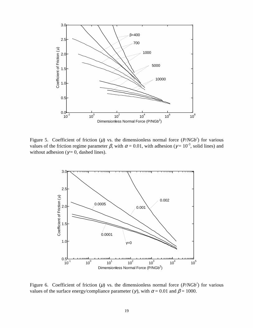
The effect of the friction regime roughness parameter β on the variation of the frictioncoefficient with normal force is shown in Fig. 5. The cases in which the adhesion effects areincluded are plotted with solid lines whereas the cases without adhesion are plotted with brokenlines. This figure shows that our model predicts higher coefficients of friction values for lower βvalues. The effect of adhesion, which is to increase the friction coefficient and the differencebetween the results with and without adhesion, is greatest for low β and low normal force. Lowβ indicates that the contacts are more likely to be in the nano region (Fig. 2) in which thefriction stress is greatest and the effect of adhesion on the contact radius is expected to be mostimportant. For high β the friction coefficient is nearly independent of adhesion and less sensitiveto normal load. A large normal force results in µ being nearly independent of both adhesion andof β. The value of µ decreases with increasing P . Although it may not at first be obvious fromFigs. 3-5, due to the scalings involved, the friction coefficient is more sensitive to α than to β.
Finally, the effect of the adhesion parameter γ on µ vs. P is plotted in Fig. 6. A baselineplot without adhesion is also given for comparison. As expected the results show that for high γ ,the model predicts higher coefficient of friction values, especially at low loads. It is noted that ineach of Figs. 4-6 the friction coefficient decreases with the applied load. Even for a zero valueof the applied normal force, the effect of adhesion can be to create a finite contact area and hencea finite friction force which leads to an infinite friction coefficient.
The dimensionless normal force vs. separation is shown in Fig. 7 for various values of and � with �= 10-3. Note that an order of magnitude increase in produces roughly a two ordersof magnitude increase in the normal force. Without adhesion P varies as
2, but with adhesionthat relation is more complex. It may appear surprising that the friction regime parameter wouldhave such a strong influence on the normal force. However from Eq. (7)
/ bσ αβ= and αβ // =bR (20)
and so 22/12/32 /bRσαβ = which, without adhesion, more explicitly shows the dependence ofthe normal force with the surface topography ( �5). The effect of increasing is to increase theQRUPDO� IRUFH� LQ� D� QHDUO\� OLQHDU�PDQQHU�� �1RWH� WKH� DSSDUHQW� GLVFRQWLQXLW\� LQ� WKH� FXUYH� IRU� � ������� � ��������,Q�WKLV�FDVH�DQG�IRU�D�VHSDUDWLRQ��G� ��RI�DSSUR[LPDWHO\������WKH�QRUPDO�IRUFHapproaches zero. For larger separations, the negative of the normal force has been plotted – theSHDN�YDOXH�RI�ZKLFK� LQGLFDWHV� WKH�SXOO�RII� IRUFH�� �1RWH� WKDW� IRU� WKH� ILYH� FDVHV�SORWWHG�RQO\� � ������� � ������JLYHV�D�WHQVLOH�IRUFH�RQ�VHSDUDWLRQ�
The dimensionless friction force vs. separation is shown in Fig. 8 for various values of and � with �= 10-3. The trend of a nearly two orders of magnitude increase in the friction forcewith an order of magnitude increase in the friction regime parameter appears at first to becounter-intuitive. Note, however, that while an increase in does cause a decrease in the frictioncoefficient (Fig. 5) it also causes an increase in both the normal and friction force due to theeffect of surface topography, i.e. Eq. (20). The effect of on the friction force is not as strong,especially at small separations for which the effect of adhesion is less.
The dimensionless average contact pressure (P/E*A) vs. normal force is shown in Fig. 9for various values of and � with �= 10-3. The real contact area (A) was computed from

12
( ) ( ) ( )2 2 2 2
d d
A N b a z dz N b z d z dzπ φ π β φ∞ ∞
= = −∫ ∫ (21)
The solid and dashed lines are with and without adhesion respectively. There is a relativelysmall change in the average contact pressure as the normal force varies over several orders ofmagnitude. The effect of adhesion is to reduce the average contact pressure by increasing thereal contact area for a given applied load. Also the results are more sensitive to α than to β,with low α (smooth surfaces) giving lower contact pressures due to a greater real contact area.
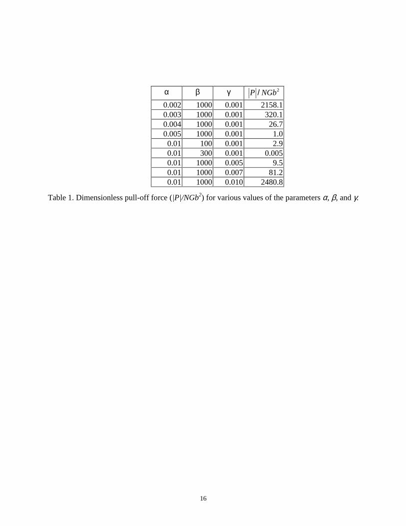
Finally Table 1 shows the dimensionless pull-off force for various values of theparameters α, β, and γ. As described in connection with Fig. 7, the pull-off force (|P|/NGb2) isthe largest magnitude of tensile force needed to separate the surfaces. For most of the materialcombinations presented, the normal force remains compressive and a pull-off force does notexist. Note that low α and high γ increase the pull-off force dramatically.
ConclusionsThe friction force measured between two bodies is the combined result of friction forces whichare present in a very large number of nano- and micro-scale asperity contacts. It is known fromrecent experiments with the AFM and SFA, that single asperity contacts yield friction stresseswhich have a constant value in the micro range (SFA) but give a constant and much higher valuein the nano range (AFM). This difference in friction stress is greater than an order of magnitude.Recent single asperity modeling efforts by Hurtado and Kim [21,22] have demonstrated amechanism which can explain this phenomenon.
In this paper, the single asperity nano contact model of Hurtado and Kim has beenincorporated into a multi-asperity model for contact and friction which includes the effect ofasperity adhesion forces using a Maugis model. Three key dimensionless parameters α, β and γhave been defined which represent surface roughness, friction regime, and surfaceenergy/compliance. Results are shown for the friction coefficient vs. the normal load, for thenormal and friction forces vs. separation, and for the average contact pressure vs. normal load,for various values of these three key dimensionless parameters. The importance of nano effectsin multi-asperity contacts are shown to be most significant for small α and/or β, high γ, and lownormal load. Future work should include the effects of scale-dependent plasticity, thin films,various distributions of asperity heights and shapes, asperity coupling, and experiments tovalidate the model.

13
References[1] Tabor, D., 1981, “Friction–The Present State of Our Understanding,” ASME Journal of
Lubrication Technology, 103, pp. 169-179.
[2] Greenwood, J.A and Williamson, J.B.P., 1966, “Contact of Nominally Flat Surfaces,”Proceedings of the Royal Society of London, A295, pp. 300-319.
[3] Hutchinson, J.W., 2000, “Plasticity at the Micron Scale,” International Journal of Solidsand Structures, 37, pp. 225-238.
[4] Johnson, K.L., 1985, Contact Mechanics, Cambridge University Press, Cambridge, UK.
[5] McCool, J.I., 1986, “Comparison of Models for the Contact of Rough Surfaces,” Wear,107, pp. 37-60.
[6] Greenwood, J.A., and Tripp, J.H., 1971, “The Contact of Two Nominally Flat RoughSurfaces,” Proceedings of the Institution of Mechanical Engineers, 185, pp. 625-633.
[7] Johnson, K. L., Kendall, K., and Roberts, A. D., 1971, “Surface Energy and the Contact ofElastic Solids,” Proceedings of the Royal Society of London, A324, pp. 301-313.
[8] Derjaguin, B. V., Muller, V. M., and Toporov, Y. P., 1975, “Effect of ContactDeformations on the Adhesion of Particles,” Journal of Colloid and Interface Science, 53,pp. 314-326.
[9] Maugis, D., 1992, “Adhesion of Spheres: The JKR-DMT Transition Using a DugdaleModel,” Journal of Colloid and Interface Science, 150, pp. 243-269.
[10] Johnson, K.L. and Greenwood, J.A., 1997, “An Adhesion Map for the Contact of ElasticSpheres,” Journal of Colloid and Interface Science, 192, pp. 326-333.
[11] Dugdale, D. S., 1960, “Yielding in Steel Sheets Containing Slits,” Journal of the Mechanicsand Physics of Solids, 8, pp. 100-104.
[12] Chang, R. W., Etsion, I., Bogy, D. B., 1987, “An Elastic-Plastic Model for the Contact ofRough Surfaces,” ASME Journal of Tribology, 109, pp. 257-263.
[13] Chang, R. W., Etsion, I., Bogy, D. B., 1988, “Adhesion Model for Metallic RoughSurfaces,” ASME Journal of Tribology, 110, pp. 50-56.
[14] Chang, R. W., Etsion, I., Bogy, D. B., 1988, “Static Friction Coefficient Model for MetalicRough Surfaces” ASME Journal of Tribology, 110, pp. 57-63.
[15] Hamilton, G.M., 1983, “Explicit Equations for the Stresses Beneath a Sliding SphericalContact,” Proceedings of the Institution of Mechanical Engineers, 197C, pp. 53-59.
[16] Fuller, K.N.G and Tabor, D., 1975, “The Effect of surface roughness on the adhesion ofelastic solids,” Proceedings of the Royal Society of London, A345, pp. 327-342.
[17] Stanley, H.M., Etsion, I. and Bogy, D.B., 1990, “Adhesion of Contacting Rough Surfacesin the Presence of Sub-Boundary Lubrication,” ASME Journal of Tribology, 112, pp. 98-104.
[18] Polycarpou, A. A., and Etsion, I.,1998, “Static Friction of Contacting Real Surfaces in thePresence of Sub-Boundary Lubrication,” ASME Journal of Tribology, 120, pp. 296-303.
[19] Carpick, R.W., Agrait, N. Ogletree, D.F. and Salmeron, M., 1996, “Measurement ofInterfacial Shear (friction) with an ultrahigh vacuum atomic force microscope,” Journal ofVacuum Science and Technology, B14, pp. 1289-1295.

14
[20] Homola, A.M, Israelachvili, J.N., McGuiggan, P.M. and Gee, M.L., 1990, “Fundamentalexperimental studies in tribology: the transition from 'interfacial' friction of undamagedmolecularly smooth surfaces to 'normal' friction with wear,” Wear, 136, pp. 65-83.
[21] Hurtado, J.A. and Kim, K.-S., 1999, “Scale Effects in Friction of Single Asperity Contacts:Part I; From Concurrent Slip to Single-Dislocation-Assisted Slip,” Proceedings of theRoyal Society of London, A455, pp. 3363-3384.
[22] Hurtado, J.A. and Kim, K.-S.,1999, “Scale Effects in Friction in Single Asperity Contacts:Part II; Multiple-Dislocation-Cooperated Slip,” Proceedings of the Royal Society ofLondon, A455, pp. 3385-3400.
[23] Adams, G.G., Müftü, S., and Mohd Azhar, N., 2002, “A Nano-Scale Multi-Asperity Modelfor Contact and Friction,” 2002 ASME/STLE Tribology Conference, Cancun, Mexico, Oct.28-30, 2002. Proceedings on CD-ROM. Paper No. ASME2002-TRIB-258.

15
List of Figures
Figure 1. The topography of a rough surface and a smooth flat surface.
Figure 2. Relationship between the dimensionless friction stress and the dimensionless contactradius according to the HK model.
Figure 3. Scaled coefficient of friction (αµ) vs. scaled normal force (P/αNGb2) for variousvalues of β, without adhesion (γ = 0).
Figure 4. Scaled coefficient of friction (αµ) vs. scaled normal force (P/αNGb2) for variousvalues of α, with γ =10-3.
Figure 5. Coefficient of friction (µ) vs. the dimensionless normal force (P/NGb2) for variousvalues of the friction regime parameter β, with α = 0.01, with adhesion (γ = 10-3, solid lines) andwithout adhesion (γ = 0, dashed lines).
Figure 6. Coefficient of friction (µ) vs. the dimensionless normal force (P/NGb2) for variousvalues of the surface energy/compliance parameter (γ ), with α = 0.01 and β = 1000.
Figure 7. Dimensionless normal force (P/NGb2) vs. dimensionless separation (σ /d), for variousvalues of α and β, and with γ = 10-3. Dashed lines indicate that the normal force is tensile.
Figure 8. Dimensionless friction force (F/NGb2) vs. dimensionless separation (σ /d), for variousvalues of α and β, and with γ = 10-3.
Figure 9. Dimensionless average contact pressure (P/E*A) vs. dimensionless normal force(P/NGb2), for various values of α and β, with γ = 10-3 (solid lines), and γ = 0 (dashed lines).
List of Tables
Table 1. Dimensionless pull-off force (|P|/NGb2) for various values of the parameters α, β, and γ.
16
Table 1. Dimensionless pull-off force (|P|/NGb2) for various values of the parameters α, β, and γ.
α β γ 2/P NGb
0.002 1000 0.001 2158.10.003 1000 0.001 320.10.004 1000 0.001 26.70.005 1000 0.001 1.00.01 100 0.001 2.90.01 300 0.001 0.0050.01 1000 0.005 9.50.01 1000 0.007 81.20.01 1000 0.010 2480.8

17
Figure 1. The topography of a rough surface and a smooth flat surface.
Figure 2. Relationship between the dimensionless friction stress and the dimensionless contactradius according to the HK model.
10-2
100
102
104
106
10-4
10-3
10-2
10-1
Dimensionless Contact Radius (a/b)
Dim
ensi
onle
ss F
rictio
n S
tres
s (τ
f /G
*)
1
2
3
z
x
Mean of surface height
Separation, dMean of asperity heights
u

18
Figure 3. Scaled coefficient of friction (αµ) vs. scaled normal force (P/αNGb2) for variousvalues of β, without adhesion (γ = 0).
Figure 4. Scaled coefficient of friction (αµ) vs. scaled normal force (P/αNGb2) for variousvalues of α, with γ =10-3.
10-5
100
105
1010
1015
0.00
0.01
0.02
0.03
0.04
Sca
led
Coe
ffici
ent o
f Fric
tion
(αµ )
Dimensionless Normal Force (P/αNGb2)
β=102
103
104
105
106
100
101
102
103
104
105
106
107
0.005
0.010
0.015
0.020
0.025
0.030
Sca
led
Coe
ffici
ent o
f Fric
tion
(αµ )
Dimensionless Normal Force (P/αNGb2)
Without Adhesion
α=0.006 0.01
0.03
0.06
19
Figure 5. Coefficient of friction (µ) vs. the dimensionless normal force (P/NGb2) for variousvalues of the friction regime parameter β, with α = 0.01, with adhesion (γ = 10-3, solid lines) andwithout adhesion (γ = 0, dashed lines).
Figure 6. Coefficient of friction (µ) vs. the dimensionless normal force (P/NGb2) for variousvalues of the surface energy/compliance parameter (γ ), with α = 0.01 and β = 1000.
10-2
100
102
104
106
108
0.0
0.5
1.0
1.5
2.0
2.5
3.0
Coe
ffici
ent o
f Fric
tion
(µ)
Dimensionless Normal Force (P/NGb2)
β=400
700
1000
5000
10000
10-1
100
101
102
103
104
105
0.5
1.0
1.5
2.0
2.5
3.0
Coe
ffici
ent o
f Fric
tion
(µ)
Dimensionless Normal Force (P/NGb2)
0.002
0.001 0.0005
0.0001
γ=0

20
Figure 7. Dimensionless normal force (P/NGb2) vs. dimensionless separation (σ /d), for variousvalues of α and β, and with γ = 10-3. Dashed lines indicate that the normal force is tensile.
Figure 8. Dimensionless friction force (F/NGb2) vs. dimensionless separation (σ /d), for variousvalues of α and β, and with γ = 10-3.
0 1 2 3 410
-2
100
102
104
106
108
Dim
ensi
onle
ss N
orm
al F
orce
(P
/NG
b2 )
Dimensionless Separation (d/σ)
α=0.01,β=10000
0.01,5000
0.05,1000
0.01,1000
0.005,1000
0 1 2 3 410
-1
100
101
102
103
104
105
106
Dim
ensi
onle
ss F
rictio
n F
orce
(F
/NG
b2 )
Dimensionless Separation (d/σ)
α=0.01,β=10000
0.01,5000
0.002,1000
0.01,1000

21
Figure 9. Dimensionless average contact pressure (P/E*A) vs. dimensionless normal force(P/NGb2), for various values of α and β, with γ = 10-3 (solid lines), and γ = 0 (dashed lines).
10-2
100
102
104
106
1080.000
0.002
0.004
0.006
0.008
0.010A
vera
ge D
imen
sion
less
Con
tact
Pre
ssur
e (P
/E* A
)
Dimensionless Normal Force (P/NGb2)
0.01,1000
α=0.02, β=1000
0.01,10000
0.005,1000