a multi-sided bézier patch with a simple control structure

EUROGRAPHICS 2016 / J. Jorge and M. Lin(Guest Editors)

Volume 35 (2016), Number 2

A Multi-sided Bézier Patch with a Simple Control Structure

Tamás Várady1 Péter Salvi1 György Karikó2

1 Budapest University of Technology and Economics2 ShapEx Ltd.

AbstractA new n-sided surface scheme is presented, that generalizes tensor product Bézier patches. Boundaries and corresponding cross-derivatives are specified as conventional Bézier surfaces of arbitrary degrees. The surface is defined over a convex polygonaldomain; local coordinates are computed from generalized barycentric coordinates; control points are multiplied by weighted,biparametric Bernstein functions. A method for interpolating a middle point is also presented.This Generalized Bézier (GB) patch is based on a new displacement scheme that builds up multi-sided patches as a combinationof a base patch, n displacement patches and an interior patch; this is considered to be an alternative to the Boolean sum concept.The input ribbons may have different degrees, but the final patch representation has a uniform degree. Interior control points—other than those specified by the user—are placed automatically by a special degree elevation algorithm.GB patches connect to adjacent Bézier surfaces with G1 continuity. The control structure is simple and intuitive; the numberof control points is proportional to those of quadrilateral control grids. The scheme is introduced through simple examples;suggestions for future work are also discussed.

Categories and Subject Descriptors (according to ACM CCS):I.3.5 [Computer Graphics]: Computational Geometry and ObjectModeling—Curve, surface, solid, and object representations

1. Introduction

The mathematical formulation of multi-sided surfaces is an impor-tant area in Computer Aided Geometric Design. There is a widevariety of these patches due to several (often contradictory) require-ments, and it is hard to find a single best representation. For exam-ple, transfinite patches constrain only some boundaries and cross-derivatives, then the patch interior is created solely from this infor-mation. Control point-based patches provide multiple local controlsfor the interior by means of a well-defined structure of 3D vectors.

The transfinite approach is helpful when we are satisfied withthe shape by the automatic settings, however, difficulties may ariseif the shape needs to be further modified or optimized in the in-terior. Control point-based schemes are attractive when the num-ber of control points is relatively low, however, if certain detailsat the boundaries require the presence of too many control points,it is hard to generate and manipulate these. Locality can be bothan advantage and a problem, depending on whether we want toedit smaller or larger parts of the surface. Another aspect is how tostitch together adjacent surfaces smoothly; here transfinite patchesmay provide simpler solutions. The efficiency of numerical compu-tations may also be a concern, and in this regard control point-basedsurfaces seem to be superior to transfinite surfaces, and the list goeson.

In this paper we propose a new control point-based surface rep-resentation, called the GB patch, which generalizes tensor prod-uct Bézier patches. It extends the mathematical elegance of Bézierpatches to an arbitrary number of sides, and allows the combina-tion of Bézier boundaries of different degrees with related crossderivatives. In some sense, we try to combine the advantages of thetransfinite schemes (e.g. [SVR14]) and conventional control point-based approaches: basically the patch is constructed from boundaryinformation, and at the same time an interior structure of controlpoints is built up in an automatic manner. These control points maybe satisfactory as they are, but can also be modified, allowing forinteractive editing or shape optimization. The input Bézier ribbonsmay have different degrees and complexity, but each can be editedseparately. The patch evolves naturally “behind the scenes”, andsmoothly blends together all information into a single entity. Inte-rior control points are inserted when and where it is necessary.

Generalized Bézier patches are rational polynomials with C∞

continuity within the patch. There is no need for artificial in-ternal subdividing structures between quadrilaterals, however—according to our best knowledge—they cannot be directly con-verted into a standard CAD format. These patches can be utilized invarious areas of CAGD: (i) Aesthetic design of complex free-formobjects is still a challenging task; this includes general topologycurve network-based design, as well. (ii) Hole filling is also an im-portant problem in various modeling situations, in particular whencomplex vertex blends are created. (iii) The approximation of 3D

c© 2016 The Author(s)Computer Graphics Forum c© 2016 The Eurographics Association and JohnWiley & Sons Ltd. Published by John Wiley & Sons Ltd.

T. Várady, P. Salvi, Gy. Karikó / A Multi-sided Bézier Patch with a Simple Control Structure

point clouds when points are located in an irregular, multi-sidedregion, is also an interesting application.

This paper is structured as follows. After reviewing previouswork in Section 2, we discuss a new approach for creating multi-sided patches that applies the displacement principle (Section 3).We introduce the Generalized Bézier patch in Section 4 with itsparameterization, control structure, and blending functions. In Sec-tion 5 the algorithm of combining Bézier surfaces of various de-grees to constitute a single GB patch is discussed. This sectioncomprises the algorithms of degree reduction and elevation for GBpatches. The paper is concluded by a few examples (Section 6), in-cluding the pros and cons of the scheme and suggestions for futurework.

2. Previous work

Multi-sided surfaces have been studied since the early 80s, see re-lated reviews in [Mal98, VRS11] amongst others. An early controlpoint-based solution appeared in Sabin’s quadratic patch [Sab83],and the cubic surface of Hosaka and Kimura [HK84]. These werelater generalized to arbitrary degrees by Zheng and Ball [ZB97]using a control net structure similar to ours. Their parameterizationmethod depends on the number of sides; solutions for 3, 5 and 6-sided patches are described in the paper. The sum of the blendingfunctions is set to 1 by compensating at the interior control points(cf. weight deficiency in our solution, see Section 4.4). The individ-ual weights are products of powers of distance parameters, whichyields an expression of much higher degree than the one proposedin Section 4.3. A subsequent publication [Zhe01] generalized thispatch for non-twist-compatible configurations.

Another line of research started with the S-patch [LD89], wherethe binomial coefficients of Bernstein polynomials were replacedby multinomials, and the (u,v) quadrilateral domain was replacedby a convex polygon with generalized barycentric coordinates.While beautiful in theory, its practical use is somewhat limited dueto the high number of control points and the special, fairly com-plex, multi-linked control structure. (For example, a 6-sided quinticS-patch requires 222 internal control points disregarding the bound-aries; our GB patch only 25.) To our best knowledge, these prob-lems have not been addressed, though a recent paper on cage defor-mation [SS15] proposes selective degree elevation for S-patches.

Warren [War92] introduced an interesting idea: multi-sided sur-faces are created by “cutting off” edges of rational Bézier trian-gles, using base points (points where all homogeneous coordinatesare 0). With this method, one can build patches of 3 to 6 sideswith a low number of control points, and the boundary curves canhave different degrees. C1 continuity to adjacent patches can alsobe achieved, but this is not so straightforward, due to the specialcontrol structure (cf. Section 4.6).

A recent publication [SZ15] explores conditions for G1 continu-ity between toric surfaces. This is a new and interesting multi-sidedpatch formulation, but the lattice structure of its control points is aconstraint that may limit its usefulness for e.g. 5-sided surfaces.

None of the above publications deals with the automatic place-ment of control points. While this can arguably be done by mini-mizing a suitable target function, there is a strong demand in design

applications to provide a default arrangement for the interior con-trol points. Our solution for GB patches will be discussed in detailsin Section 5.

Finally we should mention a special kind of n-sided patches, thatare created as a collection of rectangular patches with central split-ting. The main issues are how to create and control good subdi-viding boundaries, and how to ensure smooth connections betweenthe adjacent patches, in particular at the extraordinary center point.We can list only a few from the many interesting publications. Oneof the earliest was Gregory’s C1 bicubic solution [GZ94], followedby various biquadratic, bicubic and biquartic surface splines withG1 (e.g. [Pet94]), biseptic with G2 [LS08], and bisextic surfaceswith C2 continuity [Pra97]. A recent result in this area is a fair,quasi-G2 continuous biquartic configuration proposed in [KNP15].

The basic advantage of these methods is that they stitch togetherstandard patches, but may not have high-degree continuity alongtheir seam lines, in contrast to genuine n-sided patches, such asthe GB patch. Another aspect is that the majority of these methodsapproximate a control polyhedron, while our focus is to develop acombined scheme that interpolates a prescribed set of curves andoffer additional interior control.

In the forthcoming sections we will discuss several features thatdistinguish the proposed GB scheme from other approaches, suchas: simple control structure, ease of connecting multiple ribbonswith various degrees, intuitive method to automatically generateinterior control points (gaining further degrees of freedom), andC∞ continuity in the interior of the patch.

3. The displacement approach

The majority of transfinite patch formulations for quadrilateral andn-sided patches are based on the Boolean sum principle. BicubicCoons patches [Coo67] take two side-to-side interpolants and sub-tract a correction term that interpolates the corner positions, tan-gents, and twists. Gregory patches [Gre86] use corner interpolants,where the sum of two adjacent boundaries and cross-derivatives iscompensated by correction terms. Generalized Coons patches, pro-posed in [SVR14], are also composed by adding n side ribbons andsubtracting n corner correction terms to ensure interpolation alongthe boundaries.

Here we propose an alternative, the displacement scheme. Thebasic idea is that we define curves by separating the end constraints(positions and first derivatives) from their middle parts. For sur-faces we distinguish three parts: corner constraints (positions, tan-gents and twists), side constraints (positions and cross-derivatives),and a surface interior. We will use this approach for combiningBézier surfaces using GB patches.

Any parametric curve can be written as r(u) = rB(u) + rD(u),where rB(u) denotes the base curve, and rD(u) denotes the dis-placement curve. We assume that rB(u) interpolates the end po-sitions and end tangents, i.e., (assuming a parametric intervalof [0,1]) rB(0) = r(0), rB(1) = r(1), r′B(0) = r′(0), r′B(1) = r′(1).Let us take a simple example, see Figure 1. A quartic Bézier curve

c© 2016 The Author(s)Computer Graphics Forum c© 2016 The Eurographics Association and John Wiley & Sons Ltd.


D2D4

C3C2

C3C1 C2C4

Q0Q4

Q1Q4

Q2Q4

Q3Q4

Q4Q4

Figure 1: Displacements (red: original quartic curve, green: cubiccurve, blue: cubic curve elevated to quartic).

is given as

r(u) =4

∑i=0

Q4i B4

i (u), (1)

where Q4i are its control points. The base curve rB(u) is a cubic

curve

rB(u) =3

∑i=0

C3i B3

i (u), (2)

where C30 = Q4

0, C31 = Q4

0 +43 (Q

41−Q4

0), C32 = Q4

4 +43 (Q

43−Q4

4),and C3

3 = Q44.

After degree elevating rB(u), an identical curve of degree 4 isobtained with control points C4

i . Clearly C4i = Q4

i , except for i = 2;where C4

2 = 12 (C

31 +C3

2) 6= Q42. We define the displacement vector

D42 between the middle control points as D4

2 = Q42−C4

2 , and thusobtain a displacement curve rD(u) = D4

2B42(u). It can be seen that

rD(u) influences only the middle part of the curve and not the ends.

The same logic can be applied to n-sided surfaces, as well. Letus compose our surface as the sum of a base patch, n displacementpatches and an interior patch:

S(u,v) = SB(u,v)+n

∑i=1

SDi(u,v)+SI(u,v). (3)

The base patch interpolates the corner data, the displacementpatches act only in the middle of the sides and vanish as we movetowards the corners. The interior patch determines the surface inthe middle and vanishes as we approach the sides and the corners.

While in the Boolean sum approach correction terms are sub-tracted, in the displacement approach the sum of different surfacecomponents are taken. By switching the individual components“on” and “off”, local effects can be observed and analyzed.

4. The Generalized Bézier patch

A Generalized Bézier (GB) patch S(u,v) is generated by mappingthe (u,v) points of an n-sided convex polygonal domain Γ into 3D.We can handle patches with an arbitrary number of sides (n ≥ 3).The sides of the polygon Γi (i = 1 . . .n) are mapped to the bound-aries of the patch; each boundary is a degree d Bézier curve. Themulti-sided control net, whose structure is determined by n and d,is a straightforward extension of the control grid of quadrilateralBézier patches with degree d.

We associate certain rows of control points with individual sidesof the domain and introduce the number of control point layersl = (d + 1)÷ 2. For example, Figure 4 shows a 5-sided, degree 4control net where l = 2. Figure 5 shows a 5-sided, degree 5 controlnet where l = 3. (From the above definition it follows that thereare always two patches with a given number of layers, with degreed = 2l and d = 2l−1.)

First we introduce some elements of the GB scheme, includingcontrol net, parameterization and weight deficient blending func-tions, and then we will be able to formulate the surface equation.

4.1. Control nets

The concept of multi-sided control nets is depicted in Figure 2.First let us consider a quadrilateral control grid. For even degreesthe grid consists of a central control point and four quadrants (blackframes in Fig. 2a). For odd degrees (see Fig. 2b) a conventional gridconsists of just the four quadrants. It is a peculiar feature of the GBpatch, that its control network contains a central control point (C0)also for odd degrees. This structure can be generalized to n corners;the number of control points will be proportional to n.

Comparing the above examples with the five-sided patches ofFigures 2c and 2d, we can see that in the quartic case, the 4-sidedpatch has 4 ·6+1 = 25 control points, while the 5-sided GB patchhas 5 ·6+1 = 31 points. In the quintic case, a conventional 4-sidedpatch (with no C0) has 4 · 9 = 36 control points, while the 5-sidedGB patch has 5 ·9+1 = 46 points.

In general, for even degrees (d = 2l), the number of controlpoints is n · l(l+1)+1 for both the conventional 4-sided and the n-sided GB patches. For odd degrees (d = 2l−1), the number of con-trol points is 4l2 for the conventional 4-sided patches, and n · l2 +1for the n-sided GB patches.

4.2. Local coordinates and Bernstein blending functions

For each side of the polygonal domain we introduce local sideand distance parameters, denoted by si = si(u,v) and hi = hi(u,v),see Figure 3. These parameters are computed using Wachspressbarycentric coordinates λi = λi(u,v), i = 1 . . .n. There are sev-eral publications that thoroughly discuss the properties of gener-alized barycentric coordinates, see for example [HF06]. It is well-known that (i) λi ≥ 0 [positivity] and (ii) ∑λi = 1 [partition ofunity] hold for all points within a convex domain. Denote thevertices of the polygon by Pi and take an arbitrary point (u,v).Then (iii) (u,v) = ∑Piλi(u,v) [reproduction] holds, as well. Fi-nally, for all vertices Pj, we have (iv) λi = δi j [Lagrange property],where δi j is the Kronecker delta.

While generalized barycentric coordinates are associated withthe vertices of the polygon, the si and hi parameters of GB patchesare associated with the individual sides, inheriting important prop-erties that we will use later.

Let us define the local parameters as

si =λi

λi−1 +λi, (4)

hi = 1−λi−1−λi. (5)



(a) n = 4, d = 4 (b) n = 4, d = 5 (c) n = 5, d = 4 (d) n = 5, d = 5

Figure 2: Quadrants of quartic and quintic patches.

Pi-1 Pi

Pi-2

Pi+1

Γi

(u,v)Γi-1

Γi+1

si(λi-1,λi)

hi(λi-1,λi)

Figure 3: Multi-sided domain and parameterization.

The side parameter si varies from 0 to 1 on side i; si = 0 on side i−1, si = 1 on side i+1. For all other points, si takes values between0 and 1. The distance parameter hi vanishes on side i, since thisis the only place where the sum λi−1 +λi equals to 1. It increaseslinearly from 0 to 1 on sides i−1 and i+1. On the remaining sideshi = 1. On side i the equations si = hi−1 and si = 1−hi+1 are alsosatisfied.

Note: the above equation for si is undefined for points on the“distant” sides Γ j, j /∈ {i− 1, i, i + 1}, however, there exists anequivalent formula that resolves this problem. Introducing h⊥i−1 andh⊥i+1 as the perpendicular distances from edges Γi−1 and Γi+1, wehave

si =sin(θi)h⊥i−1

sin(θi)h⊥i−1 + sin(θi−1)h⊥i+1, (6)

where θi denotes the angle at Pi.

We are going to use degree d biparametric Bernstein blendingfunctions of (si,hi) over the domain:

Bdj,k(si,hi) =

(dj

)(1− si)

d− js ji ·

(dk

)(1−hi)

d−khki . (7)

These Bernstein functions are defined in the same way as for thequadrilateral domains with the difference that the “opposite” side(where hi = 1) will be mapped to multiple sides of the domainpolygon.

4.3. Control points of the i-th side

The control points of the i-th side are denoted by Cd,ij,k, 0 ≤ j ≤ d,

0≤ k < l. The “contribution” of the i-th side can be written as

Sdi (si,hi) =

d

∑j=0

l−1

∑k=0

µij,kCd,i

j,kBdj,k(si,hi). (8)

The µij,k-s are scalar multipliers that will ensure that the multi-

sided patch on side i is determined solely by its associated con-trol points Cd,i

j,k. In other words, neither the adjacent, nor the distantsides will have any effect on the i-th side.

It is important to notice that there are shared control pointsaround the corners that affect two adjacent sides. For example, takethe four control points (colored red) in Figure 4 that fall into boththe black and grey frames. These four control points determine theposition, the first derivatives and the mixed partial derivative (twistvector) of the patch at the corner. (For simplicity’s sake we assumetwist compatibility in this paper.) Taking the bottom side as side i,these control points occur both in the Sd

i (si,hi) and Sdi+1(si+1,hi+1)

parts, being indexed in two different ways. For the i-th side wehave Cd,i

j,k, j ∈ {d−1,d}, k ∈ {0,1}; for the (i+1)-th side Cd,i+1j,k ,

j,k ∈ {0,1}. This also means that in the final surface equationthe shared control points will actually be multiplied by a weightedcombination of Bernstein functions

µid−k, jB

dd−k, j(si,hi)+µi+1

j,k Bdj,k(si+1,hi+1), j,k ∈ {0,1}.

In Figure 4 a quartic patch is shown (l = 2) with quadruples ofshared control points. In Figure 5 a quintic patch is shown (l = 3),where 3×3 control points are shared at each corner.

Let us return to assigning weights to the control points of the i-thside. First take the quartic case in Figure 4. The four shared controlpoints at the left will be multiplied by a scalar function αi, andthose at the right by βi (see below). A weight of 1 will be assignedto the control points in the middle. Formally, we define µi

j,k as

µij,k =

k<2

αi =

hi−1hi−1+hi

j < 2,

1 2≤ j ≤ d−2,βi =

hi+1hi+1+hi

j > d−2.

(9)

This sets all µ-s to 1 on the i-th side, where hi = 0, thus producinga constant 1 multiplier for the corresponding Bernstein functions.



Figure 4: Control points of a patch with 2 layers (n = 5, d = 4).

Figure 5: Control points of a patch with 3 layers (n = 5, d = 5).

The method of assigning weights is more complicated whenl ≥ 3; an example is shown in Figure 5. All weights for k < 2 arecomputed as before. When k ≥ 2, take the diagonal j = k on theleft side (where j < l). Weights of 1

2 will be assigned to the controlpoints on the diagonal, and zeros for all the control points abovethis diagonal (where j < k). Taking the right side, another diago-nal is defined by j = d− k; the weights are assigned in a similarmanner as before. All the remaining weights of the control pointsbetween the two diagonals belong exclusively to the i-th side andwill have a weight of 1. We can formally define the k ≥ 2 case asfollows:

µij,k =

j<l

0 j < k,12 j = k,1 j > k,

µij,k =

j≥l

0 j > d− k,12 j = d− k,1 j < d− k.

(10)

4.4. Weight deficiency

For affine invariance the sum of the blending functions must be 1.In the case of GB patches, we introduce a central control point thatis multiplied by a central blending function Bd

0(u,v), that is equalto the weight deficiency of the blending functions assigned to the

other control points:

Bd0(u,v) = 1−

n

∑i=1

d

∑j=0

l−1

∑k=0

µij,kBd

j,k(si(u,v),hi(u,v)). (11)

We have found that setting the default center point to the averageof the n innermost control points is a natural choice:

C0 =1n

n

∑i=1

Cd,il,l−1. (12)

With this we can define an interior surface using the central controlpoint as

Sd0(u,v) =C0Bd

0(u,v). (13)

The central control point is useful for moving the middle point ofthe GB patch to an arbitrary location, as we will see in Section 5.3.

4.5. The patch equation

Now we are ready to formulate the equation of the GB patch. UsingEquations (8) and (13):

Sd(u,v) =n

∑i=1

Sdi (si(u,v),hi(u,v))+Sd

0(u,v). (14)

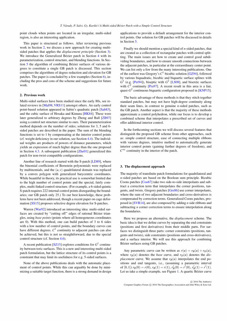
The GB patch is a convex combination of a net of control points,similarly to the tensor product Bézier patches. As shown in Fig-ure 6, the control points can be classified by their location withinthe structure. Control points around the vertices (red) are to repro-duce the positional and tangential constraints at the corners; theseare multiplied by a rational combination of two biparametric Bern-stein functions. Control points between these quadruples (green)are to reproduce boundaries and cross-derivatives; control pointsin the interior (yellow) are to produce a smooth blend between theboundaries and the interior. The latter groups of control points aremultiplied by ordinary biparametric Bernstein functions. Finally,the central control point (blue) is to adjust the interior of the GBpatch, and is multiplied by a special blend, the weight deficiency.

In the next subsection we will investigate how GB patches can beconnected to adjacent tensor product Bézier surfaces or other GBpatches with G1 continuity.

4.6. Bézier ribbons and cross-derivatives

Let us take the first two rows of control points that belong to side i:Cd,i

j,k, k < 2. Using ordinary biparametric Bernstein functions, these

define a Bézier ribbon, that determines a boundary curve rdi and a

first cross-derivative tdi along the side parameter si:

rdi (si) =

d

∑j=0

Cd,ij,0Bd

j,0(si,0), (15)

tdi (si) =

d

∑j=0

d(Cd,ij,1−Cd,i

j,0)Bdj,0(si,0). (16)

Let us take the same set of control points and apply the local pa-rameterization and the weighted Bernstein functions of GB patches.We will show that S(u,v) and S′(u,v) reproduces the boundary and



the cross-derivative along Γi. In this section x′ denotes a directionalderivative of x by an arbitrary direction in the (u,v) domain. Ourproof consists of three parts. First we show that Si(u,v) does notaffect the distant sides Γ j, j /∈ {i−1, i, i+1}, neither in positionalnor in differential sense. Then we show how Si(u,v) affects theadjacent sides Γ j, j ∈ {i− 1, i+ 1}. Finally we show that Si(u,v)reproduces the prescribed boundary functions. For this proof, it issufficient to investigate the properties of the weighted Bernstein

functions µij,kBd

j,k(si,hi) and their derivatives(

µij,kBd

j,k(si,hi))′

inthe first two rows (k < 2).

(i) The contribution of Γi does not affect the distant sides, sincethe weighted Bernstein functions and their derivatives vanish. Thisholds, because by definition hi equals 1 there, and all related blend-ing functions contain a (1−hi)

2 term.

(ii) Take the positional contributions of Γi to the adjacent sideΓi−1. (For Γi+1 we proceed in the same way.) The weighted Bern-stein functions vanish, since (a) for j < 2 the multiplier µi

j,k = 0due to hi−1 = 0, (b) the remaining Bernstein functions with j ≥ 2contain at least one si term, but si = 0 on side Γi−1.

Next look at the derivatives of the weighted Bernstein functionsof Γi on Γi−1. Those with indices j ≥ 2 have obviously no effecton Γi−1, as they contain at least one si term, and si = 0. But forj < 2 the derivatives do contribute to Γi−1:(

hi−1hi−1 +hi

Bdj,k

)′=

h′i−1hi

Bdj,k(si,hi). (17)

Similarly, the contribution to the other side (Γi+1) is(hi+1

hi+1 +hiBd

j,k

)′=

h′i+1hi

Bdj,k(si,hi). (18)

(iii) The related boundary curve will be reproduced positionallyon Γi, since the ordinary and weighted Bernstein functions becomeidentical. For 2≤ j ≤ d−2 all µi

j,k-s are constant 1; for the cornerterms, where j < 2 or j > d−2 the µi

j,k-s are also equal to 1, sincehi = 0, see Eq. (9).

In order to show the reproduction of the cross-derivative func-tion, we need to show that the derivatives of the weighted Bernsteinfunctions are identical to those of the ordinary Bernstein functions.We will take into consideration the differential terms from the Γi−1and Γi+1 sides. First take the left corner, where(

hi−1hi−1 +hi

Bdj,k

)′= Bd

j,k(si,hi)′− h′i

hi−1Bd

j,k(si,hi), (19)

while the contribution from the (i−1)-th side is

h′ihi−1

Bdd−k, j(si−1,hi−1), (20)

as can be seen by shifting the indices of Eq. (18). When hi = 0,all coefficients vanish except for Bd

j,0(si,hi) and Bdd, j(si−1,hi−1).

Fortunately hi = 1− si−1 = 0 and si = hi−1 on the i-th boundary,consequently

Bdj,0(si,hi) = Bd

d, j(si−1,hi−1), j < 2. (21)

This means that the contribution from Γi−1 cancels the second term

of Eq. (19), and only Bdj,k(si,hi)

′ remains, this is exactly what wewanted to prove. The same cancellation takes place at the othercorner due to the contribution from side Γi+1.

To sum it up, we have shown that the weighted Bernstein func-tions of S(u,v) are identical to the ordinary Bernstein functions onΓi along the boundary, i.e., the GB patch behaves as an ordinaryBézier patch having the same two rows of control points. ThusGB patches can be inserted into patchworks of quadrilateral Bézierpatches, and they can be smoothly connected to other multi-sidedGB patches.

5. Control network generation

In this section we will discuss how Generalized Bézier patches canbe used to interpolate and nicely blend Bézier ribbons of differentdegrees into a single multi-sided patch. We will show how the in-dividual ribbons can be degree elevated preserving the boundaryconstraints, and how new control points can be inserted in the inte-rior to complete the patch. These algorithms generalize the degreereduction and elevation algorithms of Bézier curves.

5.1. Degree elevation and reduction

The algorithm to degree elevate Bézier curves is well-known. Takea degree d control polygon with control points Cd

i , i = 0 . . .d. Keepthe end control points Cd+1

0 = Cd0 and Cd+1

d+1 = Cdd , and create new

interior control points on each chord of the polygon by linear inter-polation: Cd+1

i = ηiCdi−1+(1−ηi)Cd

i , where ηi =i

d+1, , i = 1 . . .d.The new curve will be a convex combination of control points usingthe Bd+1

i Bernstein functions.

Concerning the degree reduction of Bézier curves there are dif-ferent possibilities. Our preference is to perform an “inverse” de-gree elevation. In the elevation process, we have d equations to de-termine d unknowns, while in reduction we use the same equationsto determine the unknown internal control points Cd

i , i = 1 . . .d−1from the given Cd+1

i -s, but here we have one more equation thanneeded. Using index i upwards from 1, and j downwards from dwe obtain the following pairs of equations:

Cdi =

Cd+1i −ηiCd

i−11−ηi

, 1≤ i≤ k, (22)

Cdj−1 =

Cd+1j − (1−η j)Cd

j

η j, d− k+1≤ j ≤ d, (23)

where k = d÷2. We have 2k equations and d−1 unknowns, so ford = 2k+ 1 these are sufficient to determine all the interior controlpoints, but for d = 2k we obtain two different expressions for Cd

k ,and their average needs to be taken.

Degree elevation is trivial for quadrilateral Bézier patches andrelatively easy for GB patches, as well, generalizing the above al-gorithm. We retain the corner control points, and degree elevatethe boundaries by inserting new control points to each chord of theperimeter control polygons; then for each quadrilateral of the con-trol net we insert a new control point by linear interpolation. Forthe GB patches it is essential that the central control point can alsoact as a corner of a quadrilateral, so it does influence the degree



Figure 6: Degree elevation from quartic to quintic—blue lines showthe original control net. Control points are colored by classification(see Section 4.5).

elevation process. This is illustrated in Figure 6, where a quinticcontrol net was created from a quartic.

Degree elevation for GB patches basically proceeds as forquadrilateral patches. Assume we have a patch with l layers, then

Cd+1,ij,k = η jϑkCd,i

j−1,k−1 +(1−η j)ϑkCd,ij,k−1 +

η j(1−ϑk)Cd,ij−1,k +(1−η j)(1−ϑk)C

d,ij,k, (24)

where η j =j

d+1, , ϑk =k

d+1, , 1≤ j ≤ l, 1≤ k ≤ d÷2.

There are two options for setting the central control point Cd+10 :

either we compute the default central point, as was proposed inEquation (12), or we compute Cd+1

0 in such a way, that the middlesurface point stays the same. Details of the latter approach can befound in Section 5.3. We are going to use the following notation for

the degree elevation operation: Sd+1(u,v) =[Sd(u,v)

]↑.

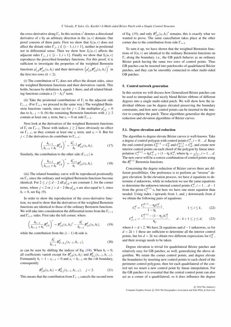
It must be emphasized that degree elevation does not producean identical GB surface, as in the case of tensor product Bézierpatches. The above procedure creates an elevated network, but theweights of the control points are computed as it was described inSection 4.3. The boundaries and cross-derivatives are preserved,of course, but the interior of the elevated patch only approximatesthe original patch. This is due to the different blending functionsand the different weight deficiencies. Figure 7a shows a 6-sidedquintic patch, and Figure 7b shows its degree elevated version witha superimposed deviation map. There are minor differences, evenwhen the middle point of the surfaces are kept identical.

Degree reduction for GB patches is also fairly straightforward,based on the related curve algorithm, so we do not go into details,

just introduce a notation: Sd(u,v) =[Sd+1(u,v)

]↓.

5.2. Creating a GB patch from Bézier ribbons

The input is a collection of Bézier ribbons with different degrees,denoted by di, i = 1 . . .n, see for example Figure 8a. We are goingto create a GB patch of degree dmax = max(di), that interpolatesand smoothly connects these ribbons. The patch will have a well-defined net of internal control points, along with a central control

(a) Original quintic patch

(b) Sextic patch with deviation

Figure 7: Deviations after elevation.

point. All control points can be used for editing or optimization.The algorithm is split into three phases.

(i) In the first phase we reduce the degrees of the individual rib-bons step by step from di to 3. Using our former notations, thecontrol points of the i-th ribbon are Cdi,i

j,k , j = 0 . . .di, k < 2. After

the first degree reduction we obtain Cdi−1,ij,k , j = 0 . . .di−1, k < 2;

then at the end C3,ij,k, j = 0 . . .3, k < 2. (Intermediate control points

are stored for later use.)

(ii) We create a base patch S3(u,v), defined by n quadruples ofcontrol points, associated with the corners. We assume that the rib-bons are compatible, i.e., although their degrees may be different,they must define the same position, tangents and twist vectors atthe corners. Consequently, after the degree reduction phase is com-pleted, a consistent cubic control net with cubic boundaries andcross-derivatives is obtained. We set the central control point C3

0(see Section 5.3) and start to build the network bottom up.

(iii) We perform degree elevations step by step for each side andcreate intermediate surfaces Md(u,v). First we compute M4(u,v) =[S3(u,v)

]↑; the degree elevated control points of the i-th ribbon are

denoted by Q4,ij,k. Then we compute the displacement vectors for all

ribbons whose degree was at least 4. These vectors will compensatethe corresponding control points of the current intermediate surfaceto reproduce all degree 4 ribbons, or partly reproduce ribbons withdegrees greater then 4. Finally we compute the degree 4 interiorcontrol points.

In general, we repeat this step several times: intermediate sur-



(a) Input Bézier ribbons (b) Reduced to cubic (base patch) (c) Elevated to quartic (d) Elevated to quintic (final patch)

Figure 8: Evolution of a GB patch.

(a) Initial configuration (b) Moving control points (c) Moving the surface center

Figure 9: Editing a GB patch.

faces are computed as Md(u,v) =[Sd−1(u,v)

]↑, then displace-

ment corrections are made where Cd,ij,k exists and the difference

vectors Cd,ij,k−Qd,i

j,k, j = 2 . . .di, k < 2 are not zero. Obviously, wenever tweak the default quadruples at the corners, since they are al-ways properly set. Then we define Cd

0 , and this completes the patchSd(u,v). After repeated degree elevations the process terminates atthe highest degree dmax.

The evolution of the GB patch is demonstrated by a simple ex-ample in Figure 8. Figure 8a shows a patch with five ribbons withdegrees 3, 4, 5, 5, and 3, respectively, starting at the bottom edgeand going in CCW direction. After degree reductions we obtain thebase patch with boundaries reduced to cubic (Figure 8b). The firstdegree elevation retains the shape of ribbons 1 and 5, reproducesthe quartic ribbon 2, and modifies ribbons 3 and 4 (Figure 8c). Thesecond degree elevation retains the shape of ribbons 1, 2 and 5, andreproduces the quintic ribbons 3 and 4. Figure 8d shows the finalquintic patch with its automatically inserted interior control points,which ensure a natural blending to connect the input ribbons.

5.3. Computing the central control point

An alternative method for computing the central control point C0allows one to specify a 3D point P0 to be interpolated by the middlepoint of the surface. Let (u0,v0) denote the center of the domainpolygon, then we want to set Sd(u0,v0) = P0. Using Equations (13)

and (14) we can reformulate this asn

∑i=1

Sdi (si(u0,v0),hi(u0,v0))+C0Bd

0(u0,v0) = P0, (25)

from which we can compute C0 as

C0 =P0−∑

ni=1 Sd

i (si(u0,v0),hi(u0,v0))

Bd0(u0,v0)

. (26)

6. Evaluation

In this section we will present a few examples and discuss thestrengths and weaknesses of the GB patch.

6.1. Example 1

The control points of GB patches can be manually edited or op-timized as in standard control point-based formulations. Figure 9ashows the curvature map of a 5-sided patch, whose control points—both in the interior and along the boundaries—have been modified;see Figure 9b. (Computing derivatives in the interior is possible, butquite complex, and thus the curvature maps here were computed us-ing a dense triangular mesh.) The user may want to explicitly setthe middle surface point to adjust the fullness of the shape. Thendegree elevation will proceed accordingly, and in each phase an ap-propriate central control point will be set to satisfy this additional



(a) Control points (b) Contouring (c) Gaussian curvature (d) Isophote lines

Figure 10: A setback vertex blend.

Figure 11: The dolphin model.

constraint. The result is shown in Figure 9c, where the first two lay-ers of the control points are the same as before, but the interior andcentral control points are relocated to force the surface to interpo-late the small red cubical marker in the middle.

6.2. Example 2

GB patches are well-suited for creating vertex blends. For exam-ple, Figure 10 shows a 6-sided setback-type vertex blend, whichconnects three edge blends with different radii. The boundary con-straints are determined by the surrounding primary and fillet sur-faces, and the fullness of the patch is also optimized by means ofthe interior control points.

6.3. Example 3

GB patches can be used to fill up general topology curve networks.The degree of the ribbons associated with the edges of the networkmay be different, but for smooth surfaces it is necessary that thetwist vectors should be compatible at the corners and G1 continu-ity is ensured between the ribbons sharing the same edge. Then theGB patches will automatically provide G1 transitions, as well. Adolphin model is shown in Figures 11–13. It consists of 12 curvesthat define eighteen faces: eight 3-sided, four 4-sided, four 5-sidedand two 6-sided surface patches. Some close-up pictures show thetop-left 6-sided patch with its ribbons (12a), full control-net (12b)and isophotes (12c). Another close-up sequence shows six patchestogether with ribbons (13a), mean curvature map (13b) and slic-ing (13c).

6.4. Example 4

The woman head in Figure 14 is a fairly complex surface modelwith many details, including the eyes, the nose and the ears. Alto-gether there are 117 curves that define 105 patches. Besides several6-sided and 3-sided patches, the important large areas are domi-nantly covered by 4-sided and 5-sided patches. This model wascreated as a collection of Generalized Bézier patches; a 5-sidedpatch—with its control-net—is shown in the middle.

6.5. Advantages/limitations and future work

The simplicity of the control structure is an attractive feature ofGB patches. Control points can be defined by means of externallayers, then the proposed method fills up the internal control pointsin a fair and predictable manner, and these can be further edited, aswell. The setting of the central control point is not an obvious issue.Our proposed default setting (see Section 4.4) is one possibility, butalternative solutions may also exist.

The GB patch inherits important properties of ordinary Bézierpatches, including affine invariance (see notes below), convex hullproperty, linear reproduction and localized effect of editing. Ourhigh-resolution numerical tests (n = 4 . . .12, d = 3 . . .12) meet theexpectations that weight deficiency is always positive. Unfortu-nately, at this point we have no algebraic proof, and this is sub-ject of future research. It must be noted, that for n = 3 the classicalbarycentric coordinates produce negative weight deficiency; nev-ertheless, 3-sided patches work nicely—see the examples. In thiscase, the middle control point is supposed to be set either by the de-fault algorithm (Section 4.4) or by interpolating a prescribed mid-dle surface point (Section 5.3). In order to ensure positive weightdeficiency for triangular surfaces, our recommendation is a simplereparametrization of the distance coordinates, similarly to the onesuggested in [SVR14].

The GB patch can be used with linear and quadratic boundaries,as well. In these cases there is only a single layer of control points,so C0 continuity is guaranteed, and the scheme remains valid.

The extension of the GB scheme to higher degree ribbons andG2 continuity, and the use of incompatible twists are subject ofongoing research; results are encouraging.

For the majority of practical applications it is sufficient that the



(a) Ribbons (b) Control points (c) Isophotes

Figure 12: Close-up of a 6-sided patch.

(a) Ribbons (b) Mean curvature (c) Slicing

Figure 13: Close-up of connected patches.

Figure 14: The face model.

GB patch intuitively interpolates the ribbons and produces a pre-dictable middle surface point, but from a mathematical point ofview it is a deficiency that this sort of degree elevation cannot re-produce the original degree d−1 patch. Our experiments show thatgood approximations by manual editing are possible; still, this isexpected to be solved by an optimization algorithm. It is an openquestion whether a scheme with perfect degree elevation exists.

The GB scheme, as all control point based schemes, is suitablefor fairing by minimizing various smoothness functionals, tweak-ing primarily the control points in the interior. Other sorts of opti-mizations are also possible, including the approximation of givenpoint sets while the boundaries are constrained. These algorithmsare subject of future research, as well.

Conclusion

A new multi-sided surface scheme has been proposed that general-izes tensor product Bézier patches, based on the displacement prin-ciple. The control net seems to be the simplest extension of con-ventional quadrilateral grids. GB patches combine Bézier ribbonswith different degrees, and build up a uniform structure with auto-matically produced interior control points. This is accomplished byspecial degree elevation and degree reduction algorithms. There ex-ists an extra degree of freedom to set the middle point of the patch,if needed.

GB patches use rationally weighted biparametric Bernstein func-tions; this explains why the most important properties of tensorproduct Bézier patches remain valid. The patches have internal C∞

continuity, it is easy to evaluate them and are well-suited for aGPU implementation. GB patches are expected to be used in vari-ous computer graphics and CAD applications including interactivegeneral topology curve network-based design, hole filling, reverseengineering and surface approximation. There are lots of challeng-ing open issues for future research.

Acknowledgments

This is a joint work by researchers at the Budapest Universityof Technology and Economics and a small technology companyShapEx Ltd., Budapest. The pictures were generated by a prototypesystem called Sketches. The dolphin model has been provided forus by Cindy Grimm (Washington University); the face model wasdesigned by Supriya Chewle (KAUST, Saudi Arabia). The projectwas partially supported by the Hungarian Scientific Research Fund(OTKA, No. 101845).



References[Coo67] COONS S. A.: Surfaces for Computer-Aided Design of Space

Forms. Tech. Rep. MIT/LCS/TR-41, Massachusetts Institute of Tech-nology, 1967. 2

[Gre86] GREGORY J. A.: N-sided surface patches. In Mathematics ofSurfaces I (1986), Oxford University Press, pp. 217–232. 2

[GZ94] GREGORY J. A., ZHOU J.: Filling polygonal holes with bicubicpatches. Computer Aided Geometric Design 11, 4 (1994), 391–410. 2

[HF06] HORMANN K., FLOATER M. S.: Mean value coordinates forarbitrary planar polygons. Transactions on Graphics 25, 4 (2006), 1424–1441. 3

[HK84] HOSAKA M., KIMURA F.: Non-four-sided patch expressionswith control points. Computer Aided Geometric Design 1, 1 (1984), 75–86. 2

[KNP15] KARCIAUSKAS K., NGUYEN T., PETERS J.: Generalizingbicubic splines for modeling and IGA with irregular layout. Computer-Aided Design (2015). 2

[LD89] LOOP C. T., DEROSE T. D.: A multisided generalization ofBézier surfaces. Transactions on Graphics 8 (1989), 204–234. 2

[LS08] LOOP C., SCHAEFER S.: G2 tensor product splines over extraor-dinary vertices. In Computer Graphics Forum (2008), vol. 27, WileyOnline Library, pp. 1373–1382. 2

[Mal98] MALRAISON P.: A bibliography for n-sided surfaces. In Math-ematics of Surfaces VIII (1998), Information Geometers, pp. 419–430.2

[Pet94] PETERS J.: Constructing C1 surfaces of arbitrary topology usingbiquadratic and bicubic splines. In Designing Fair Curves and Surfaces:Shape Quality in Geometric Modeling and Computer-Aided Design. So-ciety for Industrial and Applied Mathematics, 1994. 2

[Pra97] PRAUTZSCH H.: Freeform splines. Computer Aided GeometricDesign 14, 3 (1997), 201–206. 2

[Sab83] SABIN M.: Non-rectangular surface patches suitable for inclu-sion in a B-spline surface. In EuroGraphics (1983), North Holland,pp. 57–70. 2

[SS15] SMITH J., SCHAEFER S.: Selective degree elevation for multi-sided Bézier patches. Computer Graphics Forum 34, 2 (2015), 609–615.2

[SVR14] SALVI P., VÁRADY T., ROCKWOOD A.: Ribbon-based transfi-nite surfaces. Computer Aided Geometric Design 31, 9 (2014), 613–630.1, 2, 9

[SZ15] SUN L.-Y., ZHU C.-G.: G1 continuity between toric surfacepatches. Computer Aided Geometric Design 35–36 (2015), 255–267.Geometric Modeling and Processing 2015. 2

[VRS11] VÁRADY T., ROCKWOOD A., SALVI P.: Transfinite surfaceinterpolation over irregular n-sided domains. Computer Aided Design43, 11 (2011), 1330–1340. 2

[War92] WARREN J.: Creating multisided rational Bézier surfaces usingbase points. Transactions on Graphics 11 (1992), 127–139. 2

[ZB97] ZHENG J., BALL A.: Control point surfaces over non-four-sidedareas. Computer Aided Geometric Design 14, 9 (1997), 807–821. 2

[Zhe01] ZHENG J.: The n-sided control point surfaces without twist con-straints. Computer Aided Geometric Design 18, 2 (2001), 129–134. 2


a multi-sided bézier patch with a simple control structure

Documents