A Multi-Exchange Local Search Algorithm

for the Capacitated Facility Location Problem

Jiawei Zhang∗ Bo Chen† Yinyu Ye ‡

October 19, 2003

Abstract

We present a multi-exchange local search algorithm for approximating the capacitated facility

location problem (CFLP), where a new local improvement operation is introduced that possibly

exchanges multiple facilities simultaneously. We give a tight analysis for our algorithm and show

that the performance guarantee of the algorithm is between 3+2√

2− ε and 3+2√

2+ ε for any

given constant ε > 0. Previously known best approximation ratio for the CFLP is 7.88, due to

Mahdian and Pal (2003), based on the operations proposed by Pal, Tardos and Wexler (2001).

Our upper bound 3 + 2√

2 + ε also matches the best known ratio, obtained by Chudak and

Williamson (1999), for the CFLP with uniform capacities. In order to obtain the tight bound

of our new algorithm, we make interesting use of techniques from the area of parallel machine

scheduling.

Key words: capacitated facility location, approximation algorithm, local search algorithm.

∗Department of Management Science and Engineering, Stanford University, Stanford, CA, 94305, USA.

Email:jiazhang@stanford.edu.†Warwick Business School, The University of Warwick, Coventry, England, UK. Email:B.Chen@warwick.ac.uk.‡Department of Management Science and Engineering, Stanford University, Stanford, CA, 94305, USA.

Email:yinyu-ye@stanford.edu.

1

1 Introduction

In the capacitated facility location problem (CFLP), we are given a set of clients D and a set of

facilities F . Each client j ∈ D has a demand dj that must be served by one or more open facilities.

Each facility i ∈ F is specified by a cost fi, which is incurred when facility i is open, and by a

capacity ui, which is the maximum demand that facility i can serve. The cost for serving one unit

demand of client j from facility i is cij . Here, we wish to open a subset of facilities such that the

demands of all the clients are met by the open facilities and the total cost of facility opening and

client service is minimized. We assume that unit service costs are non-negative, symmetric, and

satisfy the triangle inequality, i.e., for each i, j, k ∈ D ∪ F , cij ≥ 0, cij = cji and cij ≤ cik + ckj .

The CFLP is a well-known NP-hard problem in combinatorial optimization with a large variety

of applications, such as location and distribution planning, telecommunication network design, etc.

Numerous heuristics and exact algorithms have been proposed for solving CFLP. In this paper,

we are concerned with approximation algorithms for the CFLP. Given a minimization problem,

an algorithm is said to be a (polynomial) ρ-approximation algorithm, if for any instance of the

problem, the algorithm runs in polynomial time and outputs a solution that has a cost at most

ρ ≥ 1 times the minimal cost, where ρ is called the performance guarantee or the approximation

ratio of the algorithm.

Since the work of Shmoys, Tardos and Aardal (1997), designing approximation algorithms

for facility location problems has received considerable attention during the past few years. In

particular, almost all known approximation techniques, including linear programming relaxation,

have been applied to the uncapacitated facility location problem (UFLP), which is a special case of

the CFLP with all ui = ∞. The best currently known approximation ratio for the UFLP is 1.517

due to Mahdian, Ye and Zhang (2002 and 2003). Furthermore, Guha and Khuller (1999) proved

that the existence of a polynomial time 1.463-approximation algorithm for the UFLP would imply

that P = NP.

On the other hand, because the (natural) linear programming relaxation for the CFLP is

known to have an unbounded integrality gap, all known approximation algorithms for the CFLP

with bounded performance guarantee are based on local search techniques. Korupolu, Plaxton

and Rajaraman (1998) is the first to show that local search algorithm proposed by Kuehn and

2

Hamburger (1963) has an approximation ratio of 8 for the case where all the capacities are uniform,

i.e., ui = u for all i ∈ F . The ratio has been improved to 5.83 by Chudak and Williamson

(1998) using a simplified analysis. When the capacities are not uniform, Pal et al. (2001) have

recently presented a local search algorithm with performance guarantee between 4 and 8.53. Their

algorithm consists of the following three types of local improvement operations: open one facility;

open one facility and close one or more facilities; close one facility and open one or more facilities.

Very recently, Mahdian and Pal (2003) reduced the upper bound to 7.88 by using operations that

combines those in Pal et al. (2001).

The main contribution of this paper is the introduction of a new type of operations, called

the multi-exchange operation, which possibly exchanges multiple facilities simultaneously, i.e., close

many facilities and open many facilities. In general, the multi-exchange operation cannot be com-

puted in polynomial time since it is NP-hard to determine if such an operation exists so that a

solution can be improved. However, we will restrict our attention to a subset of such operations

such that the aforementioned determination can be computed efficiently. We will show that the

restricted multi-exchange operation generalizes those in Pal et al. (2001).

This new type of operations enables us to approximate the CFLP with a factor of 3 + 2√

2 + ε

for any given constant ε > 0. The approximation ratio of our algorithm matches what has been

proved by Chudak and Williamson (1999) for the uniform capacity case. We also show that our

analysis is almost tight. In particular, we construct an instance of the CFLP such that the ratio of

the cost resulted from the improved local search algorithm to the optimal cost is 3 + 2√

2 − ε for

any given constant ε > 0.

The performance guarantee of our algorithm follows from a set of inequalities that is implied by

the local optimality of the solution, i.e., none of the legitimate operations can improve the solution.

The multi-exchange operations is meant to give stronger inequalities than those implied by simpler

operations. The major task of the proof is to identify those inequalities, which involves partitioning

the facilities into groups. Here, we make uses of proof techniques from the area of parallel machines

scheduling. Our proof also uses the notion of exchange graph from Pal et al. (2001).

The remainder of this paper is organized as follows. In Section 2, we present our new local

search operation together with some preliminary analyses. The performance guarantee of the

algorithm is proved in Section 3. We present the lower bound ratio example in Section 4 and then

3

make some remarks in the final section.

2 Local search algorithm

Given a subset S ⊆ F , denote by C(S) the optimal value of the following linear program LP(S):

LP(S): Minimize∑

i∈S

fi +∑

i∈S

∑

j∈Dcijxij

subject to∑

i∈S

xij = dj ∀j ∈ D∑

j∈Dxij ≤ ui ∀i ∈ S

xij ≥ 0 ∀i ∈ S, j ∈ D

where xij denotes the amount of demand of client j served by facility i. The above linear program

LP(S) is feasible if and only if∑

i∈S ui ≥∑

j∈D dj . If it is infeasible, we denote C(S) = +∞. If

it is feasible, then an optimal solution xS = (xij) and the optimal value C(S) can be found in

polynomial time.

Therefore, the CFLP is reduced to finding a subset S ⊆ F , which we simply call a solution with

service allocation xS , such that C(S) is minimized. Let Cf (S) =∑

i∈S fi and Cs(S) = C(S)−Cf (S)

denote the respective facility cost and service cost associated with solution S.

Given the current solution S, the algorithm proposed by Pal et al. (2001) performs the

following three types of local improvement operations:

• add(s): Open a facility s ∈ F\S and reassign all the demands to S∪{s} by computing xS∪{s}

and C(S ∪ {s}) using linear program LP(S ∪ {s}). The cost of this operation is defined as

C(S ∪ {s})− C(S), which can be computed in polynomial time for each s ∈ F\S.

• open(s, T ): Open a facility s ∈ F\S, close a set of facilities T ⊆ S and reassign all the

demands served by T to facility s. Demands served by facilities in S\T will not be affected.

Let the cost of reassigning one unit of demand of any client j from facility t ∈ T to facility s

be cts, which is an upper bound on the change of service cost cjs− cjt. The cost of operation

open(s, T ) is defined as the sum of (fs −∑

i∈T fi) and the total cost of reassigning demands

4

served by facilities in T to s. Pal et al. (2001) have shown that, for each s /∈ S, if there

exists a set T such that the cost of open(s, T ) is fs−α for some α ≥ 0, then one can find in

polynomial time a set T ′ such that the cost of open(s, T ′) is at most fs − (1 − ε)α for any

given ε > 0.

• close(s, T ): Close a facility s ∈ S, open a set of facilities T ⊆ F\S, and reassign all the

demands served by s to facilities in T . Demands served by facilities in S\{s} will not be

affected. Again let the cost of reassigning one unit of demand of any client j from facility s to

facility t ∈ T be cst, which is an upper bound of cjt − cjs. The cost of operation close(s, T )

is defined as the sum of (∑

i∈T fi − fs) and the total cost of reassigning demands served by

s to facilities in T . Similarly, for each s ∈ S, if there exists a set T such that the cost of

close(s, T ) is α− fs for some α ≥ 0, then one can find in polynomial time a set T ′ such that

the cost of close(s, T ) is at most (1 + ε)α− fs for any given ε > 0.

In our algorithm, we introduce an additional type of powerful restricted multi-exchange oper-

ations, which is defined below and consists of three parts.

• multi(r,R, t, T ): (i) Close a set of facilities {r} ∪R ⊆ S where r /∈ R and R may be empty;

(ii) Open a set of facilities {t} ∪ T ⊆ F\S where t /∈ T and T may be empty; (iii) Reassign

the demands served by facilities in R to facility t and the demands served by facility r to

{t} ∪ T . Recall that we let cst be the cost of reassigning one unit of demand from facility

s ∈ {r} ∪ R to facility t and crt be the cost of reassigning one unit of demand from facility

r to facility t ∈ T . Then, the cost of operation multi(r,R, t, T ) is defined as the sum of

(ft +∑

i∈T fi − fr −∑

i∈R fi) and the total cost of reassigning (according to the given rules)

demands served by facilities in {r} ∪R to facilities in {t} ∪ T .

It is clear that multi(r,R, t, T ) generalizes open(t, R ∪ {r}) by letting T = ∅. Operation

multi(r,R, t, T ) also generalizes close(r, T ∪ {t}) by letting R = ∅. However, we will still use

both notions open(t, R) and close(r, T ) to distinguish them from the more general and powerful

operation multi(r,R, t, T ). In the following lemma, we show that the restricted multi-exchange

operation can also be implemented efficiently and effectively.

5

Lemma 1. For any r ∈ S and t ∈ F\S, if there exist a set R ⊆ S and a set T ⊆ F\S such that

the cost of multi(r,R, t, T ) is A − B for some A ≥ 0 and B = fr + Σs∈Rfs, then one can find in

polynomial time sets R′ and T ′ such that the cost of multi(r,R′, t, T ′) is at most (1+ε)A−(1−ε)B

for any given ε > 0.

The ideas behind the proof of the lemma is as follows. Note that in the multi-exchange

operation multi(r,R, t, T ), all demands served by facilities in R are only reassigned to facility t.

Let d be the total amount of demand served by facilities in R. For any s ∈ S, denote by ds the

total amount of demand served by facility s in the current solution S and let ws = fs− dscst, which

is the profit of closing facility s and reassigning the demands served by s to t. We split facility t

into two, t′ and t′′, such that they are the same as facility t except that t′ has a reduced capacity

d and t′′ has a capacity ut − d and facility cost 0. Let the cost of close(r, {t′′} ∪ T ) be α− fr and

the cost of open(t′, R) be ft − Σs∈Rfs + β for some α, β ≥ 0. Then The total cost of operation

multi(r,R, t, T ) is simply the sum of these two costs (ft + α + β)− (fr + Σs∈Rfs), i.e.,

A = ft + α + β. (1)

We also have∑

s∈R

ws =∑

s∈R

fs − β. (2)

Suppose we know the value of d. Then we can perform the split of t into t′ and t′′. Since we

can approximate both operations close(r, {t′′} ∪ T ) and open(t′, R) efficiently and effectively, we

can do so also for operation multi(r,R, t, T ). Therefore, the main issue in proving Lemma 1 is to

determine d efficiently. In the following proof, we show how to locate d in one of a small number

of intervals and then use approximation.

Proof of Lemma 1. Given the constant ε > 0, let k = d1/εe. Let R0 be any set of facilities in S

such that |R0| ≤ k. We can enumerate all possible R0 in polynomial time since k is a constant. If

|R| ≤ k, then there must exist an R0 such that R0 = R, i.e., we can find R in polynomial time.

Therefore, without loss of generality we assume |R| > k and that we have found in polynomial time

R0 ⊆ R such that R0 contains k most profitable elements of R, i.e., those facilities s that have the

largest ws in R. For any S′ ⊆ S, denote d(S′) = Σs∈S′ ds and w(S′) = Σs∈S′ws.

6

Suppose first that we know the value of d(R). Consider the following knapsack problem:

Maximize∑

s∈S\(R0∪{r}) wszs

subject to∑

s∈S\(R0∪{r}) dszs ≤ d(R)− d(R0)

zs ∈ {0, 1}, ∀s ∈ S\(R0 ∪ {r})

(3)

It is evident that w(R) − w(R0) is the optimal value of the above knapsack problem. Note that,

in any optimal solution, ws ≥ 0 if zs = 1. Let S = {s ∈ S\(R0 ∪ {r} : ws ≥ 0} and m = |S|. We

index the facilities s ∈ S in order of non-increasing ws/ds and obtain S = {s1, . . . , sm}. Denote

R` = R0 ∪ {s1, . . . , s`} for any ` = 1, . . . , m.

Suppose d(Rm) > d(R). The opposite case will be dealt with very easily. Then there exists a

(unique) integer m such that 0 ≤ m < m and

m∑

i=1

dsi ≤ d(R)− d(R0) <m+1∑

i=1

dsi . (4)

Let S0 be an optimal solution to the above knapsack problem: w(S0) = w(R) − w(R0). Since

according to our indexing of elements in S,

dsiws ≤ dswsi , ∀s ∈ S0\{s1, . . . , sm+1},∀si ∈ {s1, . . . , sm+1}\S0,

summation of these inequalities, together with (4), leads to w(R)− w(R0) ≤ Σm+1i=1 wsi , i.e.,

w(R) ≤ w(Rm+1). (5)

Now we replace facility t with t, which is the same as t except that t has capacity ut −d(Rm) and facility cost 0. Recall that facility t′′ has capacity ut − d(R) and the cost of operation

close(r, T ∪{t′′}) is α− fr. By performing operation close(r, T ∪{t}) for T ⊆ F\(S ∪{t}), we can

find in polynomial time Tm such that the cost of close(r, Tm ∪ {t}) is at most (1 + ε)α− fr, since

facility t has at least the same capacity as t′′ to accommodate demands reassigned from facility r

according to the first inequality of (4). Now we claim the pair (R′, T ′) = (Rm, Tm) has the desired

approximation property as stated in the lemma.

In fact, with (5) we have

w(Rm) = w(Rm+1)− wsm+1 ≥ w(R)− wsm+1 .

7

However, by definition of R0, we have wsm+1 ≤ 1kw(R). Hence

w(Rm) ≥ (1− 1/k)w(R) ≥ (1− ε)w(R). (6)

Consequently, the total cost of multi(r,Rm, t, Tm) is at most

(ft − w(Rm)) + ((1 + ε)α− fr) ≤ ft − (1− ε)w(R) + (1 + ε)α− fr.

According to (1) and (2), the right-hand side of above is

ft − (1− ε) (Σs∈Rfs − β) + (1 + ε)α− fr ≤ (1 + ε)A− (1− ε)B.

Therefore, (Rm, Tm) is indeed a good qualified approximation of (R, T ).

If d(Rm) ≤ d(R), then it is evident that w(Rm) = w(R). Hence both (6) and the first inequality

of (4) are satisfied for m = m. Therefore, in the same way we can quickly find a qualified pair

(Rm, Tm).

Now let us drop our initial assumption for the knowledge of d = d(R), which is used in the

formulation of the knapsack problem (3). Observe that we actually need not solve (3). To obtain

the required pair (Rm, Tm), we can simple enumerate all m + 1 pairs (Ri, Ti) for i = 0, 1, . . . , m,

corresponding to all possibilities that d(R) is in one of the intervals d(Ri) ≤ d(R) < d(Ri+1) and

d (R) ≥ d(Rm). More specifically, we proceed as follows. For i = 0, 1, . . . , m, let ti be a facility that

is the same as t except that ti has capacity ut − d(Ri) and facility cost 0. Find Ti in polynomial

time by approximating the cheapest operation among all close(r, T ∪ {ti}) for T ⊆ F\(S ∪ {ti}).Among the m + 1 operations multi(r,Ri, t, Ti), i = 0, 1, . . . , m, we choose the cheapest to be used

as the required operation multi(r,R′, t, T ′).

Starting with any feasible solution S, our local search algorithm repeatedly performs the legit-

imate four types of operations defined above until none of them is admissible, where an operation

is said to be admissible if its cost is less than −C(S)/p(‖D‖, ε) with p(‖D‖, ε) = 3‖D‖/ε. Then it is

clear that the algorithm will terminate after at most O (p(‖D‖, ε) log(C(S)/C(S∗))) operations. A

solution is said to be a local optimum if none of the four legitimate operations will have a negative

cost. We summarize results in this section in the following theorem.

8

Theorem 1. The multi-exchange local search algorithm can identify and implement any admissible

operation in polynomial time for any given ε > 0. The algorithm terminates in polynomial time

and outputs a solution that approximates a local optimum to any pre-specified precision.

3 Analysis of the algorithm

Now we are ready to analyze our algorithm. Let S, S∗ ⊆ F be any local and global optimal

solutions, respectively. As is done in Korupolu et al (1998), Chudak and Williamson (1999), Pal

et al (2001), and Mahdian and Pal (2003), we will bound the facility cost Cf (S) and service

cost Cs(S) separately. As stated in Mahdian and Pal (2003), any local search algorithm with add

operation in its repertoire will guarantee a low service cost when it settles down to a local optimum,

which is summarized in the following lemma, various versions of which have been proved in the

aforementioned papers. We omit its proof here.

Lemma 2. The service cost Cs(S) is bounded above by the optimal total cost C(S∗).

Denote x(i, ·) =∑

j∈D xij . Using a simple argument of network flow, Pal, Tardos and Wexler

(2001) have proved the following.

Lemma 3. The optimal value of the following linear program is at most Cs(S∗) + Cs(S):

minimize∑

s∈S\S∗

∑

t∈S∗csty(s, t) (7)

subject to∑

t∈S∗y(s, t) = x(s, ·) ∀s ∈ S\S∗

∑

s∈S\S∗y(s, t) ≤ ut − x(t, ·) ∀t ∈ S∗

y(s, t) ≥ 0 ∀s ∈ S\S∗, t ∈ S∗.

For notational clarity, we denote c(s, t) = cst. Let y(s, t) be the optimal solution of (7).

Consider bipartite graph G = (S\S∗, S∗, E), where S\S∗ and S∗ are the two sets of nodes in the

bipartite graph and E = {(s, t) : s ∈ S\S∗, t ∈ S∗ and y(s, t) > 0} is the set of edges. Due to the

optimality of y(s, t), we can assume without loss of generality that G is a forest.

9

Consider any tree Tr of G, which is rooted at node r ∈ S∗. It is evident that the tree

has alternate layers of nodes in S∗ and in S\S∗. For each node t in this tree, let K(t) be the

set of children of t. For any t ∈ S∗ and any s ∈ S\S∗, denote y(·, t) = Σs∈S\S∗y(s, t) and

y(s, ·) = Σt∈S∗y(s, t). A facility node t ∈ S∗ is said to be weak if∑

s∈K(t) y(s, t) > 12y(·, t), and

strong otherwise.

Let us concentrate on any given sub-tree of depth at most 2 rooted at t ∈ S∗, which consists of

t, K(t) and G(t) =⋃

s∈K(t) K(s). A node s ∈ K(t) is said to be heavy if y(s, t) > 12y(·, t), and light

otherwise. A light node s ∈ K(t) is said to be dominant if y(s, t) ≥ 12y(s, ·), and non-dominant

otherwise. The set K(t) is partitioned into three subsets: the set H(t) of heavy nodes, the set

Dom(t) of light and dominant nodes and the set NDom(t) of light and non-dominant nodes (see

Figure 1 for an illustration). It is clear that if t ∈ S∗ is strong, then H(t) must be empty.

������������

������������

��������������������

��������������������

������������

������������

��������������������

��������������������

t

Heavy

s

K(s):

Light Non−dominantLight Dominant

Weak Strong

Figure 1: Facility classification

We are to present a list of legitimate operations such that (i) each facility in S\S∗ is closed

exactly once, (ii) every facility in S∗ is opened a small number of times, and (iii) the total reassign-

ment cost is not too high. Depending on their types, the nodes in S\S∗ and S∗ will be involved in

different operations.

Let us first deal with the nodes in NDom(t). For each node s ∈NDom(t), let W (s) = {t′ ∈K(s) : t′ is week} and

Rem(s) = max

y(s, t)−

∑

t′∈W (s)

y(s, t′), 0

.

10

Re-index the nodes in NDom(t) as s1, s2, · · · , sk for some k ≥ 0 (NDom(t) = ∅ if k = 0), such that

Rem(si) ≤Rem(si+1) for i = 1, . . . , k− 1. The operations given below will close si exactly once for

1 ≤ i < k. We will consider node sk together with nodes in Dom(t).

We perform operation close(si,K(si) ∪ (K(si+1)\W (si+1))) for any i = 1, · · · , k − 1. The

feasibility and costs of these operations are established in the following lemma.

Lemma 4. For i = 1, 2, · · · , k − 1, the following hold:

(i) Operation close(si,K(si) ∪ (K(si+1)\W (si+1))) is feasible, i.e., the total capacity of facil-

ities opened by the operation is at least the total capacity of those closed by the operation:

y(si, ·) ≤∑

t′∈K(si)∪(K(si+1)\W (si+1))

y(·, t′).

(ii) The cost of operation close(si,K(si) ∪ (K(si+1)\W (si+1))) is at most

c(si, t)y(si, t) +∑

t′∈W (si)

2c(si, t′)y(si, t

′) +∑

t′∈K(si)\W (si)

c(si, t′)y(si, t

′)

+ c(si+1, t)y(si+1, t) +∑

t′∈K(si+1)\W (si+1)

c(si+1, t′)y(si+1, t

′).

Proof. As illustrated in Figure 2, we note that

y(si, ·) = y(si, t) +∑

t′∈W (si)

y(si, t′) +

∑

t′∈K(si)\W (si)

y(si, t′) = Y1 + Y2 + Y3,

where Y1 = y(si, t)−∑

t′∈W (si)y(si, t

′), Y2 = 2∑

t′∈W (si)y(si, t

′) and Y3 =∑

t′∈K(si)\W (si)y(si, t

′).

We have Y2 ≤∑

t′∈W (si)y(·, t′) since W (si) is a set of weak nodes, and

Y1 ≤ Rem(si) ≤ Rem(si+1)) ≤∑

t′∈K(si+1)\W (si+1)

y(si+1, t′),

where the last inequality holds because si+1 is non-dominant. Therefore,

Y1 + Y2 + Y3 ≤∑

t′∈K(si)∪(K(si+1)\W (si+1))

y(·, t′)

The proof of (i) has suggested a way to reassign the remands from si to K(si)∪(K(si+1)\W (si+1))

as follows: Reassign y(si, t′) amount of demand to t′ for any t′ ∈ K(si)\W (si) and the cost of re-

assigning each unit is at most c(si, t′); reassign Rem(si) to t′ ∈ K(si+1)\W (si+1) and the cost of

11

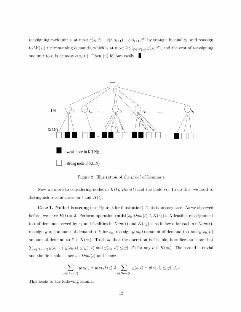
reassigning each unit is at most c(si, t) + c(t, si+1) + c(si+1, t′) by triangle inequality; and reassign

to W (si) the remaining demands, which is at most 2∑

t′∈W (si)y(si, t

′), and the cost of reassigning

one unit to t′ is at most c(si, t′). Then (ii) follows easily.

������������

������������

��������������������

��������������������

������������

������������

������������

������������

��������

��������

������������

������������

� � � �

������������

���������������

���������������

��������������������������������������������������������������������������������������������������������������������������������������������������������

��������������������������������������������������������������������������������������������������������������������������������������������������������

����������������������������������������

����������������������������������������

������������������������

������������������������

��������

��������

����������������������������������������

����������������������������������������

����������������������������������������

����������������������������������������

����������������������������������������

����������������������������������������

��������

!�!!�!!�!!�!!�!!�!!�!!�!

"�""�""�""�""�""�""�""�"

#�##�##�##�##�##�##�##�#

$�$$�$$�$$�$$�$$�$$�$$�$

%%%%%%%%

&&&&&&&&

'�'�''�'�''�'�''�'�''�'�''�'�''�'�''�'�'

(�(�((�(�((�(�((�(�((�(�((�(�((�(�((�(�(

)�)�)�)�))�)�)�)�))�)�)�)�))�)�)�)�))�)�)�)�))�)�)�)�))�)�)�)�))�)�)�)�)

*�*�*�*�**�*�*�*�**�*�*�*�**�*�*�*�**�*�*�*�**�*�*�*�**�*�*�*�**�*�*�*�*

+�+�+�++�+�+�++�+�+�++�+�+�++�+�+�++�+�+�++�+�+�++�+�+�+

,�,�,�,,�,�,�,,�,�,�,,�,�,�,,�,�,�,,�,�,�,,�,�,�,,�,�,�,

-�--�--�--�--�--�--�--�-

.�..�..�..�..�..�..�..�.

/�//�//�//�//�//�//�//�//�//�/

0�00�00�00�00�00�00�00�00�00�0

1�1�1�1�1�1�11�1�1�1�1�1�11�1�1�1�1�1�11�1�1�1�1�1�11�1�1�1�1�1�11�1�1�1�1�1�11�1�1�1�1�1�1

2�2�2�2�2�2�22�2�2�2�2�2�22�2�2�2�2�2�22�2�2�2�2�2�22�2�2�2�2�2�22�2�2�2�2�2�22�2�2�2�2�2�2

3333333

4444444

5�5�5�5�5�55�5�5�5�5�55�5�5�5�5�55�5�5�5�5�55�5�5�5�5�55�5�5�5�5�55�5�5�5�5�5

6�6�6�6�6�66�6�6�6�6�66�6�6�6�6�66�6�6�6�6�66�6�6�6�6�66�6�6�6�6�66�6�6�6�6�6

7�7�7�7�7�7�7�7�7�7�7�7�7�7�7�7�77�7�7�7�7�7�7�7�7�7�7�7�7�7�7�7�77�7�7�7�7�7�7�7�7�7�7�7�7�7�7�7�77�7�7�7�7�7�7�7�7�7�7�7�7�7�7�7�77�7�7�7�7�7�7�7�7�7�7�7�7�7�7�7�77�7�7�7�7�7�7�7�7�7�7�7�7�7�7�7�77�7�7�7�7�7�7�7�7�7�7�7�7�7�7�7�77�7�7�7�7�7�7�7�7�7�7�7�7�7�7�7�7

8�8�8�8�8�8�8�8�8�8�8�8�8�8�8�8�88�8�8�8�8�8�8�8�8�8�8�8�8�8�8�8�88�8�8�8�8�8�8�8�8�8�8�8�8�8�8�8�88�8�8�8�8�8�8�8�8�8�8�8�8�8�8�8�88�8�8�8�8�8�8�8�8�8�8�8�8�8�8�8�88�8�8�8�8�8�8�8�8�8�8�8�8�8�8�8�88�8�8�8�8�8�8�8�8�8�8�8�8�8�8�8�88�8�8�8�8�8�8�8�8�8�8�8�8�8�8�8�8

9�99�99�99�99�9

:�::�::�::�::�:

;�;;�;;�;;�;

<<<<

=====

>>>>>

?�??�??�?

@�@@�@@�@

AAAAAA

BBBBBB

C�C�C�CC�C�C�CC�C�C�CC�C�C�CC�C�C�CC�C�C�C

D�D�D�DD�D�D�DD�D�D�DD�D�D�DD�D�D�DD�D�D�D

E�E�E�E�E�EE�E�E�E�E�EE�E�E�E�E�EE�E�E�E�E�EE�E�E�E�E�EE�E�E�E�E�EE�E�E�E�E�E

F�F�F�F�FF�F�F�F�FF�F�F�F�FF�F�F�F�FF�F�F�F�FF�F�F�F�FF�F�F�F�FG�G�G�G�G

G�G�G�G�GG�G�G�G�GG�G�G�G�GG�G�G�G�GG�G�G�G�GG�G�G�G�GG�G�G�G�GG�G�G�G�GG�G�G�G�GG�G�G�G�G

H�H�H�H�HH�H�H�H�HH�H�H�H�HH�H�H�H�HH�H�H�H�HH�H�H�H�HH�H�H�H�HH�H�H�H�HH�H�H�H�HH�H�H�H�HH�H�H�H�H

s s s s s1 2 i i+1 k

t

...... ......

... ...

LN

K(LN)

: weak node in K(LN);

: strong node in K(LN).

Figure 2: Illustration of the proof of Lemma 4

Now we move to considering nodes in H (t), Dom(t) and the node sk. To do this, we need to

distinguish several cases on t and H(t).

Case 1. Node t is strong (see Figure 3 for illustration). This is an easy case. As we observed

before, we have H(t) = ∅. Perform operation multi(sk,Dom(t), t,K(sk)). A feasible reassignment

to t of demands served by sk and facilities in Dom(t) and K(sk) is as follows: for each s ∈Dom(t),

reassign y(s, ·) amount of demand to t; for sk, reassign y(sk, t) amount of demand to t and y(sk, t′)

amount of demand to t′ ∈ K(sk). To show that the operation is feasible, it suffices to show that∑

s∈Dom(t) y(s, ·) + y(sk, t) ≤ y(·, t) and y(sk, t′) ≤ y(·, t′) for any t′ ∈ K(sk). The second is trivial

and the first holds since s ∈Dom(t) and hence

∑

s∈Dom(t)

y(s, ·) + y(sk, t) ≤ 2∑

s∈Dom(t)

y(s, t) + y(sk, t) ≤ y(·, t).

This leads to the following lemma.

12

���������������

���������

���������������

���������������

���������������

���������������

���������

���������

t

Dom(t)

sk

Figure 3: Illustration of Case 1

Lemma 5. If t is strong, then operation multi(sk, Dom(t), t, K(sk)) is feasible, and the cost of

this operation is at most

∑

s∈Dom(t)

2c(s, t)y(s, t) + c(sk, t)y(sk, t) +∑

t′∈K(sk)

c(sk, t′)y(sk, t

′).

Case 2. Node t is weak and H(t) 6= ∅ (see Figure 4 for illustration). Since there can be

no more than two heavy nodes, let H(t) = {s0}. We perform operations close(s0, {t} ∪ K(s0))

and multi(sk,Dom(t), t, K(sk)). For operation multi(sk,Dom(t), t, K(sk)), the reassignment of

demands is done exactly as in Case 1. For operations close(s0, {t} ∪K(s0)), we reassign y(s0, t)

amount of demand to t and y(s0, t′) amount of demand to t′ ∈ K(s0), which is obviously feasible.

Then we have

Lemma 6. If node t is weak and H(t) = {s0}, then

(i) Operation multi(sk,Dom(t), t, K(sk)) is feasible and the cost of this operation is at most

∑

s∈Dom(t)

2c(s, t)y(s, t) + c(sk, t)y(sk, t) +∑

t′∈K(sk)

c(sk, t′)y(sk, t

′).

(ii) Operation close(s0, {t} ∪K(s0)) is feasible and its cost is at most

∑

t′∈K(s0)

c(s0, t′)y(s0, t

′) + c(s0, t)y(s0, t).

13

��������������������

������������

���������������

���������

���������

���������

���������������

���������������

���

���

���������

���������

� � � � � �

���������

Dom(t)

t

skH(t)={ s }

0

Figure 4: Illustration of Case 2

Case 3. Node t is weak and H(t) = ∅ (see Figure 5 for illustration). The analysis for this

last case is more involved. In order to find feasible operations, we need the following lemma, where

we make use of techniques from the area of parallel machine scheduling.

��������������������

������������

���������������

���������������

���������

���������

���������������

���������

������

���

���������

���������

� � �

���������

���������������

���������

t

sk g I 1I2

Dom(t)

Figure 5: Illustration of Case 3 (g = γ1 in the proof of Lemma 7).

Lemma 7. If Dom(t) 6= ∅, then there exists a node γ1 ∈ Dom(t) such that set Dom(t)\{γ1} can

be partitioned into two subsets D1 and D2 that satisfy the following:

y(γi, t) +∑

s∈Di

y(s, ·) ≤ y(·, t) for i = 1, 2,

where γ2 = sk.

14

Proof. If Dom(t) contains only one node, then we are done. We assume that Dom(t) contains at

least two nodes. First we note that

∑

s∈Dom(t)

2y(s, t) + 2y(sk, t) ≤ 2y(·, t). (8)

Initially set I1 := I2 := ∅. Let v(Ii) =∑

s∈Ii2y(s, t). Arrange the nodes in Dom(t) ∪ {sk} in a list

in non-increasing order of y(s, t). Iteratively add the first unassigned node in the list to I1 or I2

whichever has the smaller value of v(Ii) until all the nodes in the list are assigned. Based on (8),

we assume without loss of generality that Σs∈I12y(s, t) ≥ y(·, t) and∑

s∈I22y(s, t) ≤ y(·, t). Let φ

be the node last assigned to I1. It follows from (8) that

min

∑

s∈I1\{φ}2y(s, t) + y(φ, t),

∑

s∈I2

2y(s, t) + y(φ, t)

≤ y(·, t).

However, according to the way the assignment has been conducted, we have v(I1\{φ}) ≤ v(I2),

i.e.,∑

s∈I1\{φ} 2y(s, t) ≤ ∑s∈I2

2y(s, t). Therefore, the above displayed inequality implies:

∑

s∈I1\{φ}2y(s, t) + y(φ, t) ≤ y(·, t). (9)

If sk ∈ I2, then we let γ1 = φ, D1 = I1\{φ} and D2 = I2\{sk}. Then, since any node

s ∈ Dom(t) is dominant,

y(sk, t) +∑

s∈D2

y(s, ·) ≤ y(sk, t) +∑

s∈D2

2y(s, t) ≤∑

s∈I2

2y(s, t) ≤ y(·, t).

On the other hand, it follows from (9) that

y(γ1, t) +∑

s∈D1

y(s, ·) ≤ y(γ1, t) +∑

s∈D1

2y(s, t) ≤ y(·, t).

If sk ∈ I1, then let γ1 be any node in I2, let D2 = I1\{sk} and D1 = I2\{γ1}. Then,

y(γ1, t) +∑

s∈D1

y(s, ·) ≤ y(γ1, t) +∑

s∈D1

2y(s, t) ≤∑

s∈I2

2y(s, t) ≤ y(·, t).

Since sk ∈ I1 and φ is the node last assigned to I1, we have y(sk, t) ≥ y(φ, t). Hence,

y(sk, t) +∑

s∈D2

y(s, ·) ≤ y(sk, t) +∑

s∈D2

2y(s, t)

=∑

s∈I1

2y(s, t)− y(sk, t) ≤∑

s∈I1

2y(s, t)− y(φ, t).

15

Since the last term above is equal to∑

s∈I1\{φ} 2y(s, t)+ y(φ, t), the desired inequality follows from

(9), which completes our proof of the lemma.

Lemma 8. Let γi and Di (i = 1, 2) be those defined in Lemma 7. If node t is weak and H(t) = ∅,then operations multi(γi, Di, t, K(γi)) (i = 1, 2) are feasible, and their costs are respectively at most

∑

s∈Di

2c(s, t)y(s, t) + c(γi, t)y(γi, t) +∑

t′∈K(γi)

c(γi, t′)y(γi, t

′)

for i = 1, 2.

Now we are ready to provide a global picture of the impact of all the operations and demand

reassignment we have introduced, which will help bound the total facility cost of a local optimal

solution.

Lemma 9. Given any r ∈ S∗, the operations we defined on sub-tree Tr and the corresponding

reassignment of demands satisfy the following two conditions: (i) Each facility s ∈ S\S∗ is closed

exactly once; (ii) Every facility t ∈ S∗ is opened at most 3 times; (iii) The total reassignment cost

of all the operations is at most 2∑

s∈S\S∗∑

t∈S∗ c(s, t)y(s, t).

Proof. The bounds on the total reassignment cost follow from Lemmas 4,5,6 and 8. We show that

every facility t ∈ S∗ is opened at most 3 times. Note that when we take all sub-trees of Tr of depth

2 into account, any t ∈ S∗ can be the root or a leaf of such a sub-tree for at most once. If t ∈ S∗ is

strong, it will be opened once as a root and twice as a leaf. If t is weak, it will be opened at most

once as a leaf and at most twice as a root.

Theorem 2. C(S) ≤ 6Cf (S∗) + 5Cs(S∗).

Proof. Since S is locally optimal, none of the above defined operations has a negative cost. There-

fore, the total cost will also be non-negative. It follows from Lemma 9 that

3Cf (S∗\S) + 2∑

s∈S\S∗

∑

t∈S∗c(s, t)y(s, t)− Cf (S\S∗) ≥ 0.

The theorem follows from Lemmas 2 and 3.

16

Scaling the service costs cij by a factor δ = (1 +√

2)/2 and with Lemma 2 and Theorem 2,

we can show that C(S) ≤ (3 + 2√

2)C(S∗) which, together with Theorem 1, leads to the following

corollary.

Corollary 1. For any small constant ε > 0, the multi-exchange local search algorithm runs in

polynomial time with approximation guarantee of 3 + 2√

2 + ε ≤ 5.83.

4 A tight example

Figure 6 illustrates an example that gives a lower bound of our algorithm. In this example, we have

a total of 4n clients that are represented by triangles, of which 2n have demands n−1 each and the

other 2n have demands 1 each. There are a total of 4n + 1 facilities. In the current solution, the

2n open facilities are represented by squares, each of which has facility cost 4 and capacity n. The

other 2n+1 facilities are represented by circles, of which the one at the top of the figure has facility

cost 4 and capacity 2n, and each of the other 2n facilities at the bottom of the figure has facility

cost 0 and capacity n − 1. The numbers by the edges represent the unit service costs scaled by

the factor of δ = (1 +√

2)/2. Other unit service costs are given by the shortest distances induced

by the given edges. We will call a facility circle-facility or square-facility depending on how it is

represented in the figure.

We show that the current solution is a local optimum, i.e., none of the four operations will

have a negative cost. First of all, for add operation, it is easy to see that open any of the circle-

facilities would not reduce the total service cost. Secondly, notice that the connection cost between

a square-facility and a circle-facility is 0, 2, or 4. Therefore, closing any of the square-facilities would

require opening the top circle-facility, and hence any close operation will not have a negative cost.

Thirdly, we cannot open one bottom circle-facility while closing any of the square-facilities due to

the capacity constraint. Therefore, in order to open one facility and close one or many facilities,

we have to open the top circle-facility. In this case, we could possibly close any two of the square-

facilities. However, routing one unit of demand from any square-facility to the top circle-facility

will have a cost of 2. Therefore, any open operation will not be profitable. Finally, we show that

the restricted multi-exchange operation multi(r,R, t, T ) is not profitable either. We have already

shown that this is the case R = ∅ or T = ∅. Therefore, we assume that R 6= ∅ and T 6= ∅. By

17

...............

.................

.................

............

1 1 1

0

0

0 0

0 0

2n

4 4 4

n n n

4

0 00n−1 n−1 n−1

1 1

n−1 n−1n−1

11 1

facility cost

capacity

2n

1

Figure 6: A tight example with performance ratio 3 + 2√

2− ε

symmetry, we can assume r is any of the square-facilities. Since the demands served by R will be

routed to t, capacity constraint forces t to be the top circle-facility. By comparing the capacities of

the top circle-facility and the square-facilities, we know that |R| ≤ 2. Now our final claim follows

from the fact that routing one unit of demand from the square-facility to the circle-facility will cost

2. Therefore, the current solution is indeed a local optimum.

The current solution has a total facility cost of 8n and a total service cost of 2n/δ = 4n/(1+√

2)

in terms of the original (pre-scaling) data. However, if we open all the circle-facilities only, then

the total facility cost is 4 and the total service cost is 4n/(1 +√

2). The total costs of these two

solutions are 4n(3 + 2√

2)/(1 +√

2) and 4n/(1 +√

2) + 4, respectively, and their ratio approaches

3 + 2√

2 when n goes to ∞, which provides the desired lower bound of our algorithm.

5 Final remarks

A new local search algorithm for the CFLP has been proposed in this paper. The performance

guarantee of the algorithm is shown to be between 3 + 2√

2− ε and 3 + 2√

2 + ε for any constant

ε > 0. This is the currently best known approximation ratio for the CFLP. Moreover, it is the first

18

time that a tight bound of a local search algorithm for the CFLP is developed. Our result is based

not only on the introduction of a new type of multi-exchange local improvement, but also on the

exploitation of a technique from the area of parallel machine scheduling.

Several significant questions remain open. It is known that the UFLP can not be approximated

better than 1.463 in polynomial time and this lower bound naturally also applies to the more general

CFLP. But can better (larger) lower bound be established for the CFLP? On the other hand, it

would also be challenging to improve the upper bound 3 + 2√

2 + ε. In order to obtain a better

approximation ratio, it seems that new local improvement procedures are needed. Furthermore,

it is known that the natural linear programming relaxation has an unbounded integrality gap. It

would be interesting to develop new LP relaxations for the CFLP such that the known techniques

for the UFLP such as randomized rounding, primal-dual, and dual-fitting can be applied to the

CFLP.

Many other variants of the UFLP have been studied in the literature, e.g., k-median (Arya

et al 2001), multi-level facility location (Aardal, Chuak, and Shmoys 1999, Ageev, Ye, and Zhang

2003, Zhang 2004), fault-tolerant facility location (Guha, Meyerson, and Munagala 2001, Swamy

and Shmoys 2003), facility location with outlier (Charikar et al 2001). No constant approximation

ratio is known for any of these problems with capacity constraints. Since the presence of capacity

constraints is natural in practice, it would be important to study all of these problems with capacity

constraints.

References

[1] K. Aardal, F. A. Chudak and D. B. Shmoys, “A 3-Approximation Algorithm for the k-Level

Uncapacitated Facility Location Problem,”. Information Processing Letters 72(5-6): 161-167,

1999.

[2] A. Ageev, Y. Ye and J. Zhang, “Improved Combinatorial Approximation Algorithms for the

k-Level Facility Location Problem,” in Proceedings of the 30th International Colloquium on

Automata, Languages and Programming (30th ICALP), LNCS 2719, 145-156, 2003.

[3] V. Arya, N. Garg, R. Khandekar, A. Meyerson, K. Munagala and V. Pandit, “Local search

19

heuristic for k-median and facility location problems,” in Proceedings of the ACM Symposium

on Theory of Computing, 21-29, 2001.

[4] M. Charikar and S. Guha, “Improved combinatorial algorithms for facility location and k-

median problems,” in Proceedings of the 40th IEEE Foundations of Computer Science, 378-388,

1999.

[5] M. Charikar, S. Khuller, D. M. Mount and G. Narasimhan, “Algorithms for facility location

problems with outliers,” in Proceedings of the 12th Annual ACM-SIAM Symposium on Discrete

Algorithms, 642-651, 2001.

[6] G. Cornuejols, G.L. Nemhauser and L.A. Wolsey, “The uncapacitated facility location prob-

lem,” in: P. Mirchandani, R. Francis (Eds.), Discrete Location Theory, Wiley, New York,

119-171, 1990.

[7] F.A. Chudak and D.B Shmoys,“Improved approximation algorithms for the uncapacitated

facility location problem,” SIAM J. on Computing, to appear.

[8] F. A. Chudak and D. Williamson, “Improved approximation algorithms for capacitated fa-

cility location problems,” in Proceedings of the 7th Conference on Integer Programming and

Combinatorial Optimization (IPCO’99), 99-113, 1999.

[9] S. Guha and S. Khuller, “Greedy strikes back: improved facility location algorithms,” Journal

of Algorithms, 228-248, 1999.

[10] S. Guha, A. Meyerson and K. Munagala, “Improved algorithms for fault tolerant facility

location,” in Proceedings of the 12th Annual ACM-SIAM Symposium on Discrete Algorithms,

636-641, 2001.

[11] M. R. Korupolu, C. G. Plaxton and R. Rajaraman, “Analysis of a Local Search Heuristic

for Facility Location Problems,” Proceedings of the 9th Annual ACM-SIAM Symposium on

Discrete Algorithms, 1-10, 1998.

[12] A. A. Kuehn and M. J. Hamburger, “A heuristic program for locating warehouses,” Manage-

ment Science, 9:643–666, 1963.

20

[13] K. Jain, M. Mahdian, and A. Saberi, “A new greedy approach for facility location problems,”

in Proceedings of the 34th Annual ACM Symposium on Theory of Computing, 731-740, 2002.

[14] M. Mahdian and M. Pal, “Universal facility location,” in ESA 2003, to appear.

[15] M. Mahdian, Y. Ye and J. Zhang, “Improved approximation algorithms for metric facility

location problems,” in Proceedings of the 5th International Workshop on Approximation Al-

gorithms for Combinatorial Optimization (APPROX), LNCS 2462, 229-242, 2002.

[16] M. Mahdian, Y. Ye and J. Zhang, “A 2-approximation algorithm for the soft-capacitated

facility location problem,” Proceedings of the 6th International Workshop on Approximation

Algorithms for Combinatorial Optimization (APPROX), LNCS 2764, 129-140, 2003.

[17] M. Pal, E. Tardos and T. Wexler, “Facility location with hard capacities,” in Proceedings of

the 42nd IEEE Symposium on Foundations of Computer Science (FOCS), 329-338, 2001.

[18] D. B. Shmoys, “Approximation algorithms for facility location problems,” 3rd International

Workshop on Approximation Algorithms for Combinatorial Optimization (APPROX), 27-33,

2000.

[19] C. Swamy and D.B. Shmoys, “Fault-tolerant facility location,” in Proceedings of the 14th

Annual ACM-SIAM Symposium on Discrete Algorithms, 735-736, 2003.

[20] D.B. Shmoys, E. Tardos, and K.I. Aardal, “Approximation algorithms for facility location

problems,” in Proceedings of the 29th Annual ACM Symposium on Theory of Computing

(STOC), pages 265–274, 1997.

[21] J. Zhang, “Approximating the two-level facility location problem via a quasi-greedy approach,”

to appear in Proceedings of the 15th Annual ACM-SIAM Symposium on Discrete Algorithms

(SODA), 2004.

21