Accepted by IEEE Access (10.1109/ACCESS.2017.2768958)

1

Abstract—It is well known that AC power flows of a power

system do not have a closed-form analytical solution in general. This paper proposes a multi-dimensional holomorphic embedding method that derives analytical multivariate power series to approach true power flow solutions. This method embeds multiple independent variables into power flow equations and hence can respectively scale power injections or consumptions of selected buses or groups of buses. Then, via a physical germ solution, the method can represent each bus voltage as a multivariate power series about symbolic variables on the system condition so as to derive approximate analytical power flow solutions. This method has a non-iterative mechanism unlike the traditional numerical methods for power flow calculation. Its solution can be derived offline and then evaluated in real time by plugging values into symbolic variables according to the actual condition, so the method fits better into online applications such as voltage stability assessment. The method is first illustrated in detail on a 4-bus power system and then demonstrated on the IEEE 14-bus power system considering independent load variations in four regions.

Index Terms—Holomorphic embedding method, multi-dimensional holomorphic embedding method, power flow calculation, voltage stability.

I. INTRODUCTION

AST growing electricity markets and relatively slow upgrades on transmission infrastructure have pushed many

power systems to occasionally operate close to power transfer limits and raised more concerns about potential voltage instability. Voltage stability assessment is traditionally conducted by solving AC power-flow equations (PFEs) of a power system with or without contingencies. Iterative numerical methods such as the Gauss-Seidel method, Newton-Raphson (N-R) method and fast decoupled method have been widely adopted by commercialized power system software to analyze power flows and voltage stability of power systems. A major concern on these numerical methods is that the divergence of their numerical iterations is often interpreted as the happening of voltage collapse; however, theoretically speaking, does not necessarily indicate the non-existence of a

This work was supported in part by NSF grant ECCS-1610025 and SGCC Science and Technology Program under Grant 5455HJ160007.

C. Liu, B. Wang, X. Xu and K. Sun are with Department of EECS, University of Tennessee, Knoxville, TN, USA (email: cliu48@utk.edu, bwang13@vols.utk.edu, xxu30@vols.utk.edu, kaisun@utk.edu)

D. Shi is with GEIRI North America, San Jose, CA USA (email: di.shi@geirina.net).

C. L. Bak is with Department of Energy, Aalborg University, Aalborg, Denmark (email: clb@et.aau.dk)

power flow solution with acceptable bus voltages. Also, there is a probability for these numerical methods to converge to the “ghost” solutions that do not physically exist [1]. These concerns influence the performances of numerical methods especially in online applications, e.g. real-time voltage stability assessment.

As an alternative, non-iterative approach for power flow analysis, the holomorphic embedding load flow method (HELM) was firstly proposed by A. Trias in [1]-[3]. Its basic idea is to design a holomorphic function and adopt its analytical continuation in the complex plane to find an solution of PFEs. Recently, many derivative algorithms and applications based on the HELM were developed [4]-[14], such as the HELM with non-linear static load models [8], the HELM used in AC/DC power systems [9], using HELM to find the unstable equilibrium points [10], [11], network reduction [12] and the analysis of saddle-node bifurcation [13], [14].

This paper proposes a novel multi-dimensional holomorphic embedding method (MDHEM) to obtain an approximate analytic solution to PFEs. This method embeds multiple independent variables into PFEs to respectively scale power injections/consumptions of selected buses or groups of buses. Then, by means of a physical germ solution, the method represents each bus voltage as a multivariate power series of symbolic variables on the system conditions so as to derive the analytical solution expressed in a recursive form. This MDHEM has a non-iterative mechanism unlike traditional numerical methods. Its solution can be derived offline and then evaluated in real time by plugging values into symbolic variables according to the actual condition, so the method fits better into online applications for power flow or voltage stability analysis.

The rest of the paper is organized as follows. Section II introduces the conventional HELM. Section III describes the details of the proposed MDHEM including the physical germ solution, the algorithms of the MDHEM with and without PV buses, the transformations of bus types considering reactive power limits of generators, analysis on computational burdens and the details of the multi-dimensional discrete convolution algorithm that is used in the MDHEM. Section IV derives the resultant multivariate power series to multivariate Pade approximants so as to expand the region of convergence for the solution given by the MDHEM. Section V first uses a four-bus system to illustrate this method in detail and then uses the IEEE 14-bus system to verify its effectiveness and evaluate the accuracies of its analytical solutions of different

A Multi-Dimensional Holomorphic Embedding Method to Solve AC Power Flows

Chengxi Liu Member, IEEE, Bin Wang, Student Member, IEEE, Xin Xu, Student Member, IEEE, Kai Sun, Senior Member, IEEE, Di Shi, Senior Member, IEEE and Claus Leth Bak, Senior Member,

IEEE

F

Accepted by IEEE Access (10.1109/ACCESS.2017.2768958)

2

orders. Finally, conclusions are drawn in Section VI.

II. INTRODUCTION OF THE CONVENTIONAL HOLOMORPHIC

EMBEDDING LOAD FLOW METHOD

In the context of complex analysis, a holomorphic function is a complex function, defined on an open subset of the complex plane, which is continuous-differentiable in the neighborhood of every point in its domain. Define a complex function f(z) whose domain and range are subsets of the complex plane,

( ) ( ) ( , ) ( , )f z f x iy u x y i v x y (1)

where x and y are real variables and u(x, y) and v(x, y) are real-valued functions. The derivative of function f at z0 is

0

/ 00

0

( ) ( )( ) ,lim

z z

f z f zf z z

z zC

(2)

An important property that characterizes holomorphic functions is the relationship between the partial derivatives of their real and imaginary parts, known as Cauchy-Riemann condition, defined in (3). However, based on Looman-Menchoff theorem, functions satisfying Cauchy-Riemann conditions are not necessarily holomorphic unless the continuity is met [15].

0f f

ix y

(3)

The conventional HELM is founded on the theory of complex analysis, whose main advantages are its non-iterative nature. It can mathematically guarantee the convergence to a set of meaningful power flow solutions (e.g. the upper branch of the power-voltage curve on a bus) from a given correct germ solution. Additionally, assisted by Pade approximants, it is able to sufficiently and necessarily indicate the condition of voltage collapse when the solution does not exist.

For power flow calculation of a power grid having PV buses, the conventional HELM decomposes the admittance matrix Yik to a series admittance matrix Yik,tr and a shunt admittance matrix Yi,sh. Yik,tr is for the admittances between different buses, while Yi,sh is for the admittances of shunt components and off-nominal tap transformers. The advantage of this process mainly lies on the simplification of the white germ solution that has all bus voltages equal directly 1∠0 ̊ for the no-load, no-generation and no-shunt condition. See the conventional HELM of PFEs in Table I, where the 2nd and 3rd column are the original PFEs and the HELM equations for PQ, PV and slack buses respectively. The germ solution can be obtained by plugging s = 0 into expressions on the 3rd column of Table I, while the final solution of PFEs can be achieved with s = 1. Thus, under this circumstance, if the original implicit PFEs regarding voltage vectors can be transformed to the explicit form as a power series like (4), the final solution can be obtained by plugging s = 1 into the power series if only s = 1 is in the convergence region (refer to [6] for more details).

0

( ) [ ] n

n

V s V n s

(4)

There are several other methods of embedding the complex value to solve the original PFEs [7]-[10]. The embedding

method in Table I does not consider the Pload and Qload on PV buses. For more general cases with loads on generation buses, please refer [16]. The common idea of the solving process is to express each quantity embedded with s by a power series (4), e.g. V(s) and Q(s), and then equate both sides of the complex-valued equations with the same order to solve the coefficients of power series terms. Theoretically, similar to the mathematical induction method, the coefficients can be calculated term by term from low orders to high orders under a precondition that each complex-valued nonlinear holomorphic function embedded with s can be approximated by a power series in s.

TABLE I. THE EMBEDDING OF POWER FLOW EQUATIONS FOR PQ, PV AND

SLACK BUSES WITH THE CONVENTIONAL HELM

Type Original PFEs Holomorphic Embedding Method

SL ( ) SLi iV s V ( ) 1 ( 1)SL

i iV s V s

PQ *

*1

( )N

iik k

k i

SY V s

V

*

, ,* *1

( ) ( )( )

Ni

ik tr k i sh ik i

sSY V s sY V s

V s

PV

* *

1

ReN

i i ik kk

P V Y V

spi iV V

, ,* *1

( )( ) ( )

( )

Ni i

ik tr k i sh ik i

sP jQ sY V s sY V s

V s

2* *( ) ( ) 1 1spi i iV s V s V s

Fig. 1. One-line diagram of the demonstrative 3-bus system.

For the sake of simplification, use a simple three-bus system in Fig. 1 to illustrate the procedure of the conventional HELM. The system is made of one slack bus, one PQ bus and one PV bus. Quantities on both sides of the PV bus equation (i.e. column 3 and row 4 of Table I) can be replaced by power series in s as shown by (5). Then by equating both sides of (5) with the same order of sn, formula (6) is obtained to calculate the nth

terms on voltage from their (n-1)th terms.

2,

1

* *,

[0] [1] [2]

[0] [1] [0] [1] [0] [1]

N

ik tr k k kk

i i i i i i sh i i

Y V V s V s

sP j Q Q s W W s sY V V s

(5)

1* *

, ,1

1

[ ] [ 1] [ ] ( ) [ 1]N n

ik tr k i i i i i i sh ik

Y V n P W n j Q n Conv Q W Y V n

(6)

where Wi*(s) is defined as the reciprocal power series of Vi

*(s*). * * * * 2

* *

1( ) [0] [1] [2]

( )i i i ii

W s W W s W sV s

(7)

Thus, given the germ solution V[0] = 1 for this embedding method, the coefficients of Wi

*[n] can be calculated by the convolution between W*(s) and V*(s*).

Accepted by IEEE Access (10.1109/ACCESS.2017.2768958)

3

* *

1* * * *

0

[0] 1 [0] for 0

[ ] [ ] [ ] [0] for 1

i i

n

i i i i

W V n

W n W V n V n

(8)

Similarly, the coefficients of Q(s) can also be solved by the convolution between W*(s) and Q(s) based on (6). Finally, the s-embedded PFEs of this three-bus system can be separated into the real part and imaginary part, and expressed as the mathematical induction form, where the nth term on the left hand side is dependent on the 1st to (n-1)th terms on the right hand side of the equation (9).

1

1

21 21 22 23 23 2

21 21 22 23 23 2

31 31 32 33 33 3

31 31 32 33 33 3

0 1 1

1*

2 2 21

1 [ ]

1 [ ]

0 [ ]

1 [ ]

0 [ ]

0 [ ]

1

0

Re [ 1] (

re

im

im

re

im

SLn n

n

V n

V n

G B B G B Q n

B G G B G V n

G B B G B V n

B G G B G V n

V

P W n j Conv Q

*2 2, 2

2221

* * 222 2 2 2 2, 2

132

* *3 3 3, 3 32

* *3 3 3, 3

0

0) 1

Im [ 1] ( ) 1

Re 1 1

Im 1 1

sh

ren

sh

sh

sh

W Y V nG

V nBP W n j Conv Q W Y V nG

S W n Y V n B

S W n Y V n

(9)

In (9), V2re[n] is the real part of the PV bus, also dependent on the 1st to (n-1)th terms of V2, expressed as (10),

21

2 *2 0 1 2 2

1

1 1[ ] [ ] [ ]

2 2

sp n

re n n

VV n V V n

(10)

where δni is Kronecker delta function that equals 1 only for the order i = n and vanishes for other orders.

1 if

0 otherwiseni

n i

(11)

III. THE PROPOSED MULTI-DIMENSIONAL HOLOMORPHIC

EMBEDDING METHOD

Theoretically, given enough precision digits in numeric arithmetic, a conventional HELM can find the power flow solution at one required operating condition with high accuracy using the power series with a number of terms. However, the main drawback is that it does not give the expression of the power flow solution at any other operating condition, so the explicit expression is not for the whole solution space of the PFEs.

The proposed new MDHEM first finds a physical germ solution, which serves as an original point in the solution space instead of a virtual germ solution with voltage 1∠0.̊ In this way, it can extend from the physical germ solution by endowing the embedded variables with physical meanings, e.g. the loading scales to control the loading levels of load buses. Each loading scale can be either bound with each power, each load or each group of loads. A detailed procedure of the MDHEM is introduced as follows.

A. Physical Germ Solution

The proposed physical germ solution is an original point of the solution at an operating condition with physical meaning. Theoretically, any power flow solution can be defined as a physical germ solution. In this paper, the physical germ

solution is the operating condition in which each load bus (PQ bus) has neither load nor generation and each generator bus (PV bus) has specified active power output with reactive power output adjusted to control the voltage magnitude to the specified value. Such a physical germ solution has two advantages although other germ solutions can also be defined. First, it represents a condition having no load at all PQ buses. Second, the embedded variables can represent physical loading scales starting from zero and extendable to the whole solution space. If such a solution violates transmission capacity limits or bus voltage limits of the network, an acceptable light-load condition whose PQ buses have low consumptions may be used as a physical germ solution.

Fig. 2. The procedure of finding the physical germ solution.

Therefore, to find the physical germ, the s-embedded equations on PQ buses, PV buses and SL buses are expressed as in (12)-(14) respectively, where notations with subscript gi indicates the physical germ solution of bus i and S, P, V stand for the set of slack buses, PQ buses and PV buses, respectively.

( ) ,SLgi iV s V i S (12)

1

( ) 0,N

ik gkk

Y V s i

P (13)

* *

1

2 2 2* *

( )( )

( ) ,

( ) ( )

Ngi gi

ik gkk gi

spgi gi STi i STi

sP jQ sY V s

V s i

V s V s V V V s

V

(14)

The physical germ solution can be found by two steps illustrated in Fig. 2. The first step is to assume all PV and PQ buses injecting zero power to the network and find the initial voltage VSTi of every PV or PQ bus, which is indicated by Point A in Fig. 2(a) for a PV bus and Fig. 2(b) for a PQ bus. VSTi is calculated by (15)-(16).

,SLSTk kV V k S (15)

1

0,N

ik STkk

Y V k

S (16)

The second step is to replace “0” in (16) by injected reactive power as a form of s-embedded function, i.e. Qgi(s), for all PV buses to control their voltage magnitudes from the starting voltage |VSTi| towards the specified voltage |Vi

sp|, i.e. point B in Fig. 2(a). Meanwhile, the active power of each PV bus is controlled to the specified value, i.e. PGi.

Substitute power series for Vgi(s) and Wgi(s) in (13) and (14) and expand them as (17) and (18) for PQ buses and PV buses, respectively.

2

1

[1] [2] 0,N

ik STk gk gkk

Y V V s V s i

P (17)

Accepted by IEEE Access (10.1109/ACCESS.2017.2768958)

4

2

1

2 * *

2 * * * 2

2 2 2

[1] [2]

[1] [2] [0] [1],

[1] [2] [1] [2]

N

ik STk gk gkk

Gi gi gi gi gi

STi gi gi STi gi gi

sp

STi i STi

Y V V s V s

sP j Q s Q s W W si

V V s V s V V s V s

V V V s

V

(18)

Equate the coefficients of s, s2,… up to sn on both sides of (17) and (18), and then obtain Vgi[n], Wgi[n] and Qgi[n] by the terms 0 to n-1 of Wgi(s) and Qgi(s) from (19) and (20) for PQ buses and PV buses, respectively.

1

[ ] 0,N

ik gkk

Y V n i

P (19)

1* * *

1 1

* *

[ ] [ 1] [ ] [0] [ ] [ ],

[ ] [0] [ ] [0] [ 1]

N n

ik gk Gi gi gi gi gi gik

gi gi gi gi i

Y V n P W n j Q n W Q W ni

V n V V n V n

V

(20) where the voltage error of PV bus εi[n-1] is defined by (21). It will quickly converge within a small number of terms n, since it contains the high order terms of Vgi[n]sn.

12 2 *1

1

1 1[ 1] [ ] [ ]

2 2

nsp

i n i STi gi gin V V V V n

(21)

In (20), Vgi[n] and Wgi[n] are unknown complex numbers, and Qgi[n] is an unknown real number. Move all unknowns of the nth order coefficients to the left hand side and also break the PFEs into the equations respectively about real and imaginary parts. Then, a matrix equation similar to (9) is created containing all Vgi[n], Wgi[n] and Qgi[n]. Given the N-bus network with s slack buses, p PQ buses and v PV buses, the total number of equations is increased from 2s+2p+2v of (9) to 2s+2p+5v since a complex valued power series W(s) and a real valued power series Q(s) are added for each PV bus. The above method of finding a physical germ solution multiplies the active power generation at each PV bus by s and no-load at each PQ bus. If such a no-load germ solution does not exist due to the transmission capacity limits or bus voltage limits mentioned above, then an acceptable light-load condition may be used that sets a low active load Pli≠0 at each PQ bus. Then the number of equations is extended to 2s+4p+5v since W(s) is also added for each PQ bus. A 3-bus system is used to illustrate how to find a physical germ solution in detail in Appendix-B.

B. From Single-Dimension to Multi-Dimension

The conventional HELM only embeds one s into PFEs, so it may be considered a single-dimensional method. As a major drawback, it scales all loads in the system uniformly at the same rate. Loads cannot decrease, keep constant or grow at separate rates. Also, the power factor of each load is fixed. Therefore, its solutions are unable to cover all the operating conditions. Ref. [23] proposes a bivariate holomorphic embedding method, which extends the single-dimensional HELM to a two-dimensional method.

This paper proposes an MDHEM to obtain a wide variety of power flow solutions in the space about multiple embedded variables, i.e. s1, s2, …, sD. Here D is the number of dimensions. The analytical expression is derived from a physical germ solution by defining embedded variables as

individual scaling factors. For instance, each sj (j = 1~D) can control the scale of the active power or reactive power of either one load or a group of loads of interests. Thus, the conventional HELM is a special case of the MDHEM. In the following, the MDHEM will firstly be presented for a power network without PV bus and then the MDHEM for general networks will be introduced in next sub-sections.

Suppose a network has D dimensions to scale, so a D-dimensional HEM is defined in (23), where the embedding can be done by scaling each sj separately,

*

1 21 1 2

( , , , , , ) , ( , , , , , )

Nj i

ik k j Dk i j D

s SY V s s s s i

V s s s s

P (23)

where Vi(s1,s2,…,sj,…,sD) is the multivariate power series on bus i voltage given by (24). Its reciprocal is another multivariate power series Wi(s1,s2,…,sj,…,sD).

1

1

1 2 1 10 0 0

1 2

-dimensions

2 21 1 2 2

( , , , , , ) [ , , , , ]

[0, 0, , 0] [1,0, , 0] [0,1, , 0]

[2, 0, , 0] [1,1, , 0] [0, 2 ,0]

j D

D j

nn ni j D j D j D

n n n

i i i

D

i i i

V s s s s V n n n s s s

V V s V s

V s V s s V s

(24) The conventional single-dimensional HELM has three

properties [3], which needs to be verified for a multi-dimensional HEM as well.

1) Scale Invariance of the MDHEM As shown by (25), if every voltage Vk(s1,s2,,…,sj,…,sD) is

scaled to Vk’=ηVk, the resulting equations can be recovered to

the same form just with scaled injection Si by sj=|η|2. Therefore, scaling the power injection is equivalent to scaling all voltages by the same factor, which satisfies the property of scale invariance.

*

1 2

*1

1 2

2 *

1 2 *1

1 2

( , , , , , )

( , , , , , ) /

( , , , , , ) , ( , , , , , )

Nk j D i

ikk

i j D

Ni

ik k j Dk

i j D

V s s s s SY

V s s s s

SY V s s s s i

V s s s s

P

(25)

2) Holomorphicity of the MDHEM According to the generalized Cauchy-Riemann equations,

if a multivariate continuous function f(z1, z2, …, zn) defined in domain UCn satisfies (26) for each zλ, then f(z1, z2, …, zn) is holomorphic.

*0

f

z

(26)

This is also known as Wirtinger’s derivative, meaning that the function f has to be independent of zλ* for holomorphicity. Obviously, Vi in (23) does not depend on any si

* since

1

1

* * * * * *1 2 1 2

1 10 0 0

( , , , , , ) ( , , , , , )

[ , , , , ] j D

D j

i j D i j D

nn nj D j D

n n n

V s s s s V s s s s

V n n n s s s

(27)

A detailed proof of holomorphicity with the D-dimensional HEM is given in Appendix-A.

3) Reflection Condition of the MDHEM Since the complex conjugate of Vi unnecessarily preserves

Accepted by IEEE Access (10.1109/ACCESS.2017.2768958)

5

holomorphicity unless (27) holds. Under that circumstance, an image equation on conjugates should be added to (23), i.e.

*

1 2 *1

1 2

**1 2

1 1 2

( , , , , , )( , , , , , )

( , , , , , )( , , , , , )

Nj i

ik k j Dk

i j D

Nj i

ik i j Dk i j D

s SY V s s s s

V s s s s

s SY V s s s s

V s s s s

(28)

where 1 2( , , , , , )k j DV s s s s and *

1 2( , , , , , )i j DV s s s s are two sets

of independent holomorphic functions and should be conjugates of each other. Each sj must be a real value for any physical solution. Their solutions can both exist only if eq. (29) holds:

* * * * * *1 2 1 2( , , , , , ) ( , , , , , )i j D i j DV s s s s V s s s s (29)

Hence, the reflection condition is verified. After verifications of the above properties, the following

equation can be obtained from (23) and (24) with power series appear on both sides.

1 2

1

* * * *1 2

[0,0, 0] [1, 0, , 0] [0,1, , 0]

[0,0, 0] [1, 0, , 0] [0,1, , 0]

N

ik k k kk

j i i i i

Y V V s V s

s S W W s W s

(30)

Let M = n1+n2+…+nD denote the order of recursion, so Vk[0,0,…,0] is the physical germ solution for M = 0. Equate both sides of (30) and then extend the matrix equation to the Mth order as (31), where V1 is the slack bus.

1 1 1

2 1 2

1 1

* * *2 2

[ ,0, 0] [ 1,1,0, 0] [0,0, ]

[ ,0, 0] [ , , ] [0,0, ]

[ , , ]

[ , , ] [0,0, ]

[ ,0, 0] [ 1,1,0, 0] [0,0, ]

0 0 0 0 0

[ 1,0, 0]

col

k j

ik k jN N

k j N

N N N N N

i

V M V M V M

V M V n V M

Y V n

V n V M

V M V M V M

S W M S

*

* *3

* *

* *

[ 2,1, 0] 0

0 [ 1,0, 0] 0

0 0 [ , 1, ] 0

0 0 [0,0, 1]

i

i

i i j

N N

W M

S W M

S W n

S W M

(31)

Unlike the matrix equation of the conventional HELM, the

number of its columns denoted by Ncol is a D-polytope number expanding with the increase of order M. For a D-dimensional HEM at the Mth order,

1

11 !

1 ! ! 1 !

M D

i Mcol

i M DN

D M D

. (32)

Take a 2-D HEM for example. A 2-bus system with one slack bus and one PQ bus is demonstrated. s1 and s2 are selected to scale the active and reactive powers of the PQ bus, respectively. The Mth recursion of the matrix calculation is

1 1 1 1 2 1

1 1 1 1 2 1

2 2 2 1 2 221 21 22 22

2 2 221 21 21 22 4 4

[ ,0] [ 1,1] [ , ] [0, ]1 0 0 0

[ ,0] [ 1,1] [ , ] [0, ]0 1 0 0

[ ,0] [ 1,1] [ , ] [0, ]

[ ,0] [ 1,1]

re re re re

im im im im

re re re re

im im im

V M V M V n n V M

V M V M V n n V M

V M V M V n n V MG B G B

V M V M VB G G G

1 2 2 4 ( 1)

* * * *2 2 2 2 1 2 2 2 1 2 2 2

* * * *2 2 2 2 1 2 2 2 1 2 2 2

4 ( 1)

[ , ] [0, ]

0 0 0

0 0 0

Re [ 1,0] Re [ 1, ] [ , 1] Re [0, 1]

Im [ 1,0] Im [ 1, ] [ , 1] Im [0, 1]

im M

M

n n V M

PW M PW n n jQ W n n jQ W M

PW M PW n n jQ W n n jQ W M

(33)

where the 2-D discrete convolution between W(s1,s2) and

V(s1,s2) from 0 to M-1 is equal to 1. Therefore, the (M-1)th order of W[n1,n2] can be calculated from the obtained terms 0 to M-1 of V[n1,n2]. The matrix equation is divided into real and imaginary parts to be in consistent with the network with PV buses. The details of multi-dimensional discrete convolution used to calculate W[n1,n2] are described below.

C. Multi-Dimensional Discrete Convolution

For the transition towards a multi-dimensional HEM and calculation of W[n1,n2,…, nD] in (31), the single-dimensional discrete convolution on the right hand side of (9) needs to be replaced by multi-dimensional discrete convolution, which refers to rolling multiplications of two functions (e.g. f and g) on an high-dimensional lattice to produce a third function. Generally, “*” is used for the convolution operation. The number of dimensions in the given operation is reflected in the number of “*”. Take the D-dimensional HEM for example. A D-dimensional convolution is written as (34) and can be computed by summating products of corresponding terms.

1 2

1 2 1 2 1 2

1 1 2 2 1 2

, , , , * * , ,

, , , , ,D

D

D D D

D D D

y n n n f n n n g n n n

f n n n g

(34)

Different from the conventional multi-dimensional convolution taking terms from negative infinity to positive infinity, the D-dimensional convolution used in the MDHEM only keeps the 1st to (n-1)th terms. Therefore, the convolutions of W[n1,n2] on the right hand side of (33) are calculated by multiplication of two n-dimensional arrays. Fig. 3 illustrates the 1-, 2- and 3-dimensional discrete convolutions of term 0 to term 2, in which the blue and red lattices move and overlap with each other.

Fig. 3. The illustration of W*V(2,2,…,2) (a) 1-dimensional (b) 2- dimensional (c) 3- dimensional discrete convolution.

The convolution is the summation of multiplications between geometrically super-positioned red lattices and blue lattices. The discrete convolution for higher dimensions is similar but in higher-dimensional spaces.

Accepted by IEEE Access (10.1109/ACCESS.2017.2768958)

6

1 2

1 2

1

1 21, 1~

1 1 1

1 1 2 2 1 21 1 1

( )[ , , , ]

[ , , , ] [ , , ]

i i

i

D

D

k n

Dk i D

n n n

D D D

Conv W V k k k

W k k k V

， (35)

D. Multi-Dimensional HEM with PV buses

For a N-bus network with v PV buses, the PFEs for PV buses are in (36), with reactive power Q(si) also represented as a form of multivariate power series but with real coefficients

1 21 2 * * * *

1 1 2

( , , , )( , , , ) ,

( , , , )

Ni i D

ik k Dk i D

P jQ s s sY V s s s i

V s s s

V (36)

The following equation is thus obtained from (36), where multivariate power series appear on both sides.

1 21

1 2

* * *1 2

[0,0, 0] [1, 0, , 0] [0,1, , 0]

[0,0, 0] [1,0, , 0] [0,1, , 0]

[0,0, 0] [1, 0, , 0] [0,1, , 0]

N

ik k k kk

i i i i

i i i

Y V V s V s

P j Q Q s Q s

W W s W s

(37)

Then, (37) can be reformed to a recursive function about Vk[n1,n2,…,nD].

* *1 2 1 2 1 2

1

1* *

1 2 1 21, 1~

[ , , , ] [ , , , ] [0, 0, 0] [ , , , ]

[ , , , ] [0, 0, 0] ( )[ , , , ]i i

i

N

ik k D i i D i i Dk

k n

i D i i Dk i D

Y V n n n PW n n n jQ W n n n

jQ n n n W j Conv Q W k k k

(38)

where Qi[0,0,…,0] and Wi[0,0,…,0] are the obtained reactive power and the reciprocal of the voltage of the physical germ solution. Note that in (38), Vk[n1,n2,…,nD] also depends on extra unknowns W*

i[n1,n2,…,nD] and Qi[n1,n2,…,nD] of the same order. Thus three additional equations need to be added after all unknowns are moved to the left hand side: two for real and imaginary parts of W*

i[n1,n2,…,nD] and the third for the real value of Qi[n1,n2,…,nD]. For each PQ bus in the D-dimensional HEM, only one D-dimensional discrete convolution W*V is induced. However, for each PV bus in the D-dimensional HEM, three D-dimensional discrete convolutions, i.e. Q*W*, W*V and V*V* are induced. As an example, the 3-bus system in Fig. 1 for the MDHEM, having one slack bus, one PQ bus and one PV bus, is introduced in detail in Appendix-C.

E. Considering Reactive Power Limits

Reactive power limits of generators introduce discontinuity into the holomorphic functions. That is addressed in the proposed MDHEM as following. Let QGiMin and QGiMax represent the upper and lower limits of the reactive power output QGi of the generator at bus i. If QGi(s)<QGiMin or QGi(s)>QGiMax happen, the type of bus i is changed from PV to PQ and its the reactive power output is then fixed at the violated limit. Since the PFEs lose holomorphicity due to such discontinuity, the MDHEM needs to be rebuilt and resolved with altered bus types. In fact, the proposed MDHEM can predict violations of reactive power limits at PV buses beforehand from Q(si) with tested values of si.

Finally, the whole MDHEM flowchart for finding a power flow solution considering reactive power limits on PV buses is shown in Fig. 4.

F. Computer Resources Required by the MDHEM

The computational resources depend on the computation burden, i.e. the number of steps necessary to solve the problem, as well as memory space, i.e. the amount of required memory storage. For a D-dimensional HEM applied to an N-bus network with s slack buses, p PQ buses and v PV buses, Ncol terms in eq. (32) are needed to find a solution in the form of Mth-order multivariate power series. Put the unknown coefficients for Mth order power series on the left hand side and known variables on the right hand side of a matrix equation. Therefore, the left hand side of the matrix equation is a (2s+2p+5v)×(2s+2p+5v) extended admittance matrix multiplies with a (2s+2p+5v)×Ncol matrix for the unknown coefficients. The right hand side of the matrix equation is also a (2s+2p+5v)×Ncol matrix. For an Mth order truncation of the multivariate power series, the number of coefficients for each of V(si), W(si) and Q(si) is

0

1 !

! 1 !

M

termm

m DN

m D

. (39)

Fig. 4. The procedure of finding analytical solution of PFEs using the MDHEM.

7

Here, V(si) and W(si) are complex valued and Q(si) are real valued. The memory to save each of their elements depends on the digits of precision used in calculation, e.g. an element in the double-precision floating-point format taking 8 bytes. Sparse techniques can help reduce memory usage.

Most of computation burden is with multi-dimensional discrete convolution, which has totally (p+3v)×Ncol terms for the Mth order matrix equation. Each convolution involves (M-1)D-1 multiplications. However, that can be significantly speeded up by using the row-column decomposition [17] or direct matrix multiplication based on Helix transform [18], [19].

IV. MULTIVARIATE PADE APPROXIMANTS

The above-mentioned procedure can create truncated multivariate power series for all the quantities, such as voltage Vi(s1, s2, …, sD) and reactive power Qi(s1, s2, …, sD). Each multivariate power series has its convergence region, in which the power series can converge to the actual power flow solution. However, by just summing up these truncated power series, the convergence region usually can not be extended to the edge of the solution space about s1, s2, …, sD, especially close to the voltage stability boundary. The Pade approximants method is an effective tool to significantly extend the convergence region. According to Stahl’s theory, the diagonal Pade approximants can ensure the maximum analytic continuation of a power series to approximate an analytical function [20], [21].

For a bivariate power series, the method of Chisholm approximants is adopted to calculate the coefficients of a bivariate Pade approximants [22]. For example, ref. [23] uses the Chisholm approximants in a two-dimensional HEM. For more general multivariate power series, the multivariate Pade approximants (MPA) method is introduced in [24] and will be used in the proposed MDHEM.

Let f(s1, s2, …, sD) be a function of D variables approached by a formal power series expansion.

1 2

1 2

1 2 1 2 1 20 0 0

( , , , ) [ , , , ] D

D

n n nD D D

n n n

f s s s c n n n s s s

(40)

Then the Pade approximants to f(s1, s2, …, sD) is

1 2

1 2

1 2

1 2

1 2 1 20 0 0

/ 1 2

1 2 1 20 0 0

[ , , , ]

( , , , )[ , , , ]

D

D

D

D

L L Ln n n

D Dn n n

L L D L L Ln n n

D Dn n n

a n n n s s s

f s s sb n n n s s s

(41)

where L=L’ for the diagonal MPA and a[n1,n2,…,nD] and b[n1,n2,…,nD] are coefficients of term s1

n1s2n2…sD

nD in the numerator and denominator, respectively. Easily from (40) and (41), there is

1 1

1 1

1 1

1 1

1 1 1 10 0 0 0

1 1 10 0 2

[ , , ] [ , , ]

[ , , ]

D D

D D

D D

D D

L Ln n n n

D D D Dn n n n

L Ln n n n

D D Dn n n n L

b n n s s c n n s s

a n n s s o s s

(42) in which “o()” eqauls the sum of higher-order terms, representing the truncation error of [L/L]th order Pade

approximants. Since the orders of each si in both the numerator and

denominator in (41) are from 0 to L, a total number of 2(L+1)D coefficients need to be determined.

At the origin S0 in Fig. 5, the term 0 of eq. (42) satisfies [0,0, ,0] [0,0, ,0] [0,0, ,0]

:[0,0, ,0] 1

b c a

b

S0

(43)

Therefore, the remaining 2(L+1)D-2 unknown coefficients still need a number of 2(L+1)D-2 equations.

The following three sets of equations, i.e. eq. (44)-(46), are necessary for determining the remaining 2(L+1)D-2 unknown coefficients. Eq. (44) includes (L+1)D-1 equations defining coefficients in Zone S1, in which all intermediate variables τi are between 0 and L except for the original point (all τi are 0). Eq. (45) has L(L+1)D-1 equations defining the coefficients regarding τi in Zone S2. The additional (L+1)D-1-1 coefficients are defined by (46) to obtain the final unique solution. Fig. 5(a) and Fig. 5(b) showcase the zones regarding τi for two-variable and three-variable diagonal Pade approximants, respectively. More details can be found in [24].

1

1

1 1 1 10 0

1

: [ , , ] [ , , ] [ , , ],

for 0 and 0

D

D

D D D Dn n

i D

b n n c n n a

L

S1

(44)

1

1

1 1 10 0

1 2

: [ , , ] [ , , ] 0,

for 1 or 1 or or 1

D

D

D D Dn n

D

b n n c n n

L L L

S3

(45)

1

1

1 1 10 0

1 1 1

2 1 1

: [ , , ] [ , , ]

[ , , ] [ , , ] 0

for 2 1 or or 2 1

D

D

D D Dn n

D D D

D D

b n n c n n

b n n c n n

L L

S4

(46)

Fig. 5. Zones for (a) two-variable (b) three-variable diagonal MPA.

V. CASE STUDY

A. Demonstration on 4-bus Power System

Fig. 6. One-line diagram of the 4-bus power system

As shown in Fig. 6, a 4-bus system is first used to illustrate

8

the MDHEM by two cases. In Case 1, Bus 1 is the slack bus with fixed voltage 1.02pu,

Bus 2 and Bus 3 are load buses, and Bus 4 is a generator bus maintaining its voltage magnitude at 0.98pu. Loads at Bus 2 and Bus 3 are scaled by independent s1 and s2 embedded into PFEs, respectively. The MDHEM is implemented in MATLAB using MATPOWER toolbox, which takes 1.04 sec to obtain the result with maximum error of all bus voltages less than 10-8 for this 2-D MDHEM. Comparably, it takes 24.1 sec to screen the load flow of all scenarios by using the N-R method. The result is a 14th order multivariate power series (i.e. M = 14) and the terms of orders up to 2 are given in Table II.

TABLE II. Result of multivariate power series for Bus 2, 3, 4 (M<=2)

Bus  V[0,0]  V[1,0]  V[1,0]  V[2,0]  V[1,1] V[0,2]

V2 9.9510-1

+6.86110-2i -2.46510-2

-5.89410-2i 2.24810-3

-1.83310-2i -3.23210-3 +6.56210-6i

-1.33810-3 -1.98210-4i

-2.45810-4 -4.74510-4i

V3 1.005

+4.37910-2i 1.96210-3

-1.60110-2i -3.51010-2 -5.43610-2i

-3.13810-4 -3.87210-4i

-1.10710-3 +1.60010-4i

-3.75310-3 +2.76310-5i

V4 9.72710-1

+1.19710-1i 5.32310-3

-4.32610-2i 3.01210-3

-3.17910-2i -8.47810-4 -1.04710-3i

-1.27710-3 -1.29110-3i

-4.26110-4 -8.23410-4i

Fig. 7 shows the results of bus voltages by evaluating the

multivariate power series obtained by the MDHEM and compares the results with those from the N-R method at intervals of si=0.2.

Fig. 7. Comparison of results with PV bus between N-R and MDHEM.

Fig. 8. Difference between MDHEM and N-R in Case 1 with PV bus.

Fig. 8 shows the difference between the results from the N-R and MDHEM. Although the continuous power flow can also

used here to circumvent the convergence issue, the result is assigned to 0 here for simplicity if the N-R does not converge. The non-convergence of N-R does not theoretically signify the non-existence of a power flow solutions. It can be observed that in the N-R’s convergence region, the solutions from the MDHEM show great consistency. The maximum error of bus voltages is 6.52210-2pu at Bus 3 that appears very close to the edge of voltage collapse, and the multivariate power series generated by HDHEM has much less error in most of the region before voltage collapse.

Fig. 9 shows the results of bus voltages by evaluating the MDHEM using the MPA, which are also compared with the results of the N-R method calculated at intervals of si=0.2. Notice that for the voltages of two PQ buses, i.e. V2 and V3 in Fig. 9(b) and Fig. 9(c), the singularities of the MPA expression approach the actual edge of voltage collapse. Fig. 10 shows the difference between the results from the N-R and the MDHEM with MPA. The maximum difference of all bus voltages is reduced to 2.22110-2pu at Bus 3.

Fig. 9. Comparison of results with PV bus between N-R and MDHEM with multivariate Pade approximants (MDHEM+MPA).

Fig. 10. Difference between MDHEM and N-R in Case 1 with PV bus.

Fig. 11 shows the convergence region with the voltage error bound of 10-8 with order M = 14. It can be noticed that the MPA can significantly improve the convergence region.

9

Fig. 11. Convergence region with error bound of 10-8 for V2 and V3.

Fig. 12 shows the maximum voltage error of the PQ buses in the 2D space by using the multivariate power series and MPA. The error decreases by using a higher-order multivariate power series and the MPA can further extend the convergence region. Note that, the 1st order power series analytical solution is equivalent to the linear approximation of load flow solution.

Fig. 12. Maximum error of V2 and V3 in the 2D-space w.r.t. the order M.

Fig. 13. Comparison of results without PV bus between N-R and MDHEM.

In Case 2, with the increase of loading scales at load buses, the reactive power injection at the generator bus (Bus 2) violates its upper limit of 100MVar. The PV bus will be

transformed to a fixed PQ bus. Fig. 13 shows the results of bus voltages from the multivariate power series compared with the results of the N-R method. Fig. 14 shows their difference. It can be observed that V4 is no longer a PV bus with fixed voltage magnitude and the convergence region is smaller than that in Case 1. The maximum error increases to 0.0529pu at Bus 2 without the voltage support from PV buses.

Fig 14 shows the comparison of reactive powers and voltage magnitudes for Case 1 and Case 2. In Fig. 15(a), the reactive power surface of the PV bus follows a multivariate nonlinear function. Its intersection with the reactive power surface of the PQ bus determines the reactive power boundary with respect to different loading scales (i.e. s1 and s2). In Fig. 15(b), outside the “Qlim boundary”, the voltage of the PV bus type is higher than that of the PQ bus type, since PV bus type is able to maintain the voltage of Bus 4. The MDHEM can clearly tell the reactive power boundary in the multi-dimensional space about scaling factors si.

Fig. 14. Difference between MDHEM and N-R Case 2 without PV bus.

Fig. 15. The (a) reactive power and (b) voltage of PV bus for Case 1 and 2.

B. Demonstration on the 14-bus Power System

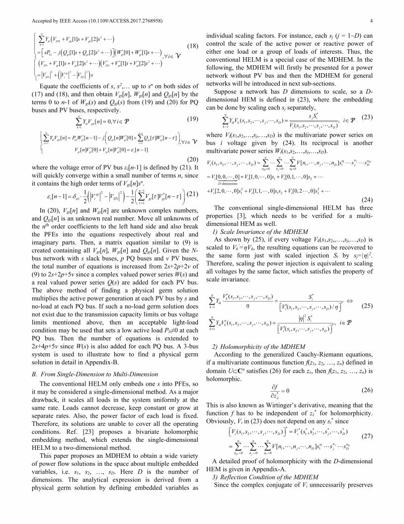
The MDHEM is also demonstrated on the IEEE 14-bus test system. The number and meanings of embedded variables can be defined arbitrarily. Here, we group all buses geographically into 4 areas with respective loading scales s1, s2, s3 and s4, as shown in Fig. 16. Then, a 4-dimensional MDHEM is performed and the result of a 11th order 4-D multivariate power series is obtained in 12.56 sec in MATLAB with the error tolerance 110-8 pu. However, it takes 121.01 sec to screen all the 4-D scenarios by using the N-R method in MATLAB.

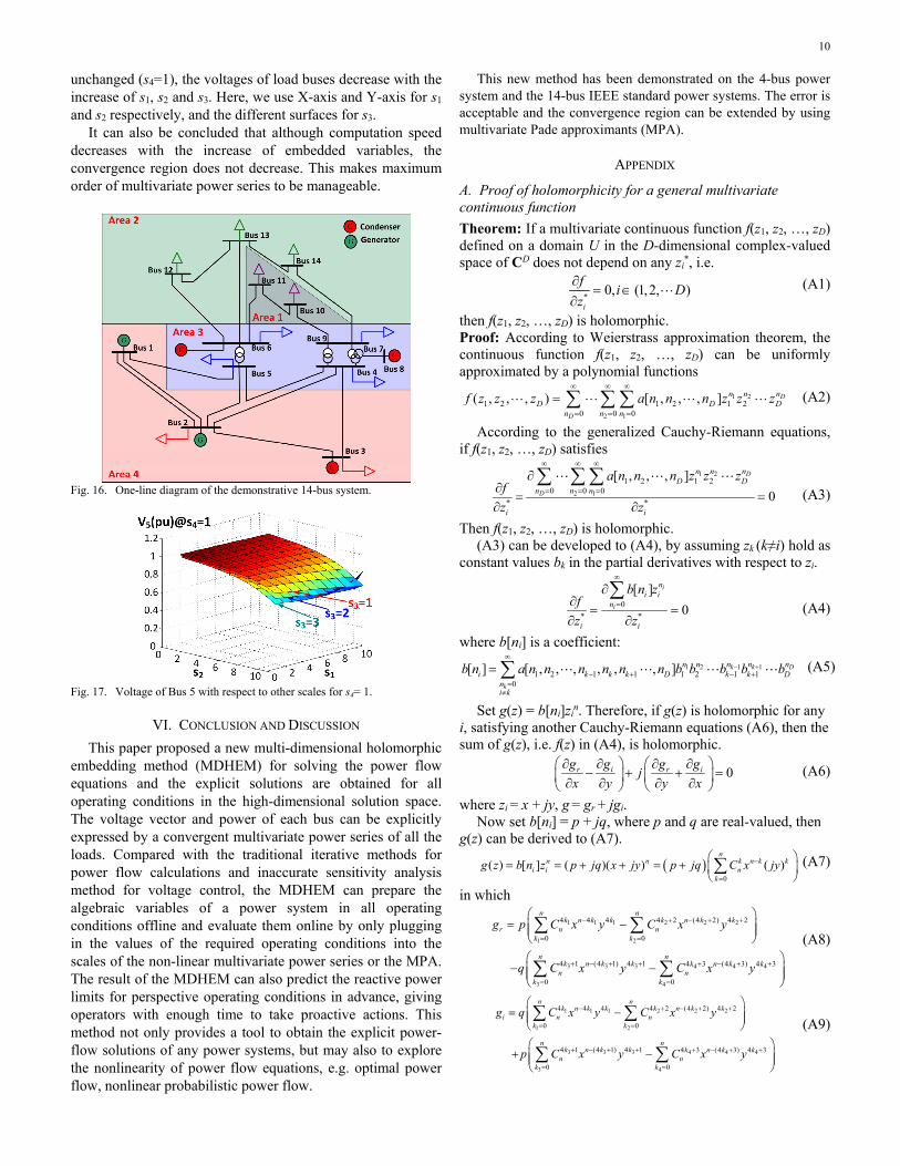
A load bus, i.e. Bus 5, is arbitrarily selected to observe the voltage with respect to s1, s2, s3 and s4, as shown in Fig 17. Other bus voltages are similar. Keeping the load of Area 4

10

unchanged (s4=1), the voltages of load buses decrease with the increase of s1, s2 and s3. Here, we use X-axis and Y-axis for s1 and s2 respectively, and the different surfaces for s3.

It can also be concluded that although computation speed decreases with the increase of embedded variables, the convergence region does not decrease. This makes maximum order of multivariate power series to be manageable.

Fig. 16. One-line diagram of the demonstrative 14-bus system.

Fig. 17. Voltage of Bus 5 with respect to other scales for s4= 1.

VI. CONCLUSION AND DISCUSSION

This paper proposed a new multi-dimensional holomorphic embedding method (MDHEM) for solving the power flow equations and the explicit solutions are obtained for all operating conditions in the high-dimensional solution space. The voltage vector and power of each bus can be explicitly expressed by a convergent multivariate power series of all the loads. Compared with the traditional iterative methods for power flow calculations and inaccurate sensitivity analysis method for voltage control, the MDHEM can prepare the algebraic variables of a power system in all operating conditions offline and evaluate them online by only plugging in the values of the required operating conditions into the scales of the non-linear multivariate power series or the MPA. The result of the MDHEM can also predict the reactive power limits for perspective operating conditions in advance, giving operators with enough time to take proactive actions. This method not only provides a tool to obtain the explicit power-flow solutions of any power systems, but may also to explore the nonlinearity of power flow equations, e.g. optimal power flow, nonlinear probabilistic power flow.

This new method has been demonstrated on the 4-bus power system and the 14-bus IEEE standard power systems. The error is acceptable and the convergence region can be extended by using multivariate Pade approximants (MPA).

APPENDIX

A. Proof of holomorphicity for a general multivariate continuous function

Theorem: If a multivariate continuous function f(z1, z2, …, zD) defined on a domain U in the D-dimensional complex-valued space of CD does not depend on any zi

*, i.e.

*0, (1,2, )

i

fi D

z

(A1)

then f(z1, z2, …, zD) is holomorphic. Proof: According to Weierstrass approximation theorem, the continuous function f(z1, z2, …, zD) can be uniformly approximated by a polynomial functions

1 2

2 1

1 2 1 2 1 20 0 0

( , , , ) [ , , , ] D

D

n n nD D D

n n n

f z z z a n n n z z z

(A2)

According to the generalized Cauchy-Riemann equations, if f(z1, z2, …, zD) satisfies

1 2

2 1

1 2 1 20 0 0

* *

[ , , , ]

0

D

D

n n nD D

n n n

i i

a n n n z z zf

z z

(A3)

Then f(z1, z2, …, zD) is holomorphic. (A3) can be developed to (A4), by assuming zk (k≠i) hold as

constant values bk in the partial derivatives with respect to zi.

0

* *

[ ]

0

i

i

ni i

n

i i

b n zf

z z

(A4)

where b[ni] is a coefficient:

1 11 21 2 1 1 1 2 1 1

0

[ ] [ , , , , , , ] k k D

k

n nn n ni k k k D k k D

ni k

b n a n n n n n n b b b b b

(A5)

Set g(z) = b[ni]zin. Therefore, if g(z) is holomorphic for any

i, satisfying another Cauchy-Riemann equations (A6), then the sum of g(z), i.e. f(z) in (A4), is holomorphic.

0i ir rg gg gj

x y y x

(A6)

where zi = x + jy, g = gr + jgi. Now set b[ni] = p + jq, where p and q are real-valued, then

g(z) can be derived to (A7).

0

( ) [ ] ( )( ) ( )n

n n k n k ki i n

k

g z b n z p jq x jy p jq C x jy

(A7)

in which

1 1 1 2 2 2

1 2

3 3 3 4 4 4

3 4

4 4 4 4 2 (4 2) 4 2

0 0

4 1 (4 1) 4 1 4 3 (4 3) 4 3

0 0

n nk n k k k n k k

r n nk k

n nk n k k k n k k

n nk k

g p C x y C x y

q C x y C x y

(A8)

1 1 1 2 2 2

1 2

3 3 3 4 4 4

3 4

4 4 4 4 2 (4 2) 4 2

0 0

4 1 (4 1) 4 1 4 3 (4 3) 4 3

0 0

n nk n k k k n k k

i n nk k

n nk n k k k n k k

n nk k

g q C x y C x y

p C x y C x y

(A9)

11

So the real part of Cauchy-Riemann equations (A6) is zero by setting k1 = k3 – 1 and k2 = k4 – 1.

0ir gg

x y

(A10)

Similarly, it can be proved the imaginary part of (A6) is also 0.

0ir gg

y x

(A11)

Therefore, g(z) is holomorphic, then f(z1, z2, …, zD) is also holomorphic.■

B. Example-1: Physical germ solution of the 3-bus system

A 3-bus system, shown in Fig. 1, is adopted to demonstrate the procedure of finding the physical germ solution. The first step is to calculate the initial no-load no-generation condition (Point A in Fig. 2). Only the slack bus propagates its voltage to the whole passive network.

11

1 1

21 21 22 22 23 23 2

21 21 22 22 23 23 2

31 31 32 32 33 33 3

31 31 32 32 33 33 3

Re1

1 Im

0

0

0

0

SL

ST re

SLST im

ST re

ST im

ST re

ST im

VV

V VG B G B G B V

B G B G B G V

G B G B G B V

B G B G B G V

(A12)

The second step is to find the physical germ solution by a simple embedding, i.e. 3rd column in TABLE I. The right hand side of the PQ bus (i.e. Bus 3) is 0, since no-load condition is held for the physical germ solution. Thus, the embedding of PV bus (i.e. Bus 2) is needed to gradually adjust its voltage magnitude to the specified value |V2pv

sp|.

1* * *

2 2 2 2 2 21 1

1 2 2* * *2 2 2 2 1 2 2

1

[ ] [ 1] [ ] [ ] [ ]

1 1[ ] [ ] ( )

2 2

N n

ik gk G g g ST g gk

nsp

ST g g ST n pv ST

Y V n P W n jQ n W j Q W n

V V n V n V Conv V V V V

-

(A13) where δni is Kronecker delta function defined by (11).

Separate the real and imaginary parts of the matrix equation and put all the nth order terms (i.e. the unknowns) to the left hand side and leave terms 0 to (n-1) (i.e. the knowns) the right hand side. The matrix equation is extended by adding Wg2(s) and Qg2(s) to the left hand side. The error of physical germ in PFE will quickly converge to 0 just in several recursions, since the deviation of voltage at PV Bus 2 contains high order terms of Vg2(s). There is (A14).

C. Example-2: MDHEM for the 3-bus system

Assume that s1 and s2 scale the active and reactive powers of the PQ bus respectively. The matrix equation for Mth order is shown correspondingly in (A15), where n1+n2=M.

21 21 22 22 23 23 2

21 21 22 22 23 23 2

31 31 32 32 33 33

31 31 32 32 33 33

2 2 2 2

2 2 2 2

2 2

1 0 0 0 0 0 0 0 0

0 1 0 0 0 0 0 0 0

0 0

0 0

0 0 0

0 0 0

0 0 0 0 0

0 0 0 0 0

0 0 0 0 0 0 0

ST im

ST re

ST re ST im ST re ST im

ST im ST re ST im ST re

ST re ST im

G B G B G B W

B G B G B G W

G B G B G B

B G B G B G

W W V V

W W V V

V V

1

1

2

2

3

3

2

2

2

1*

2 2 2 21

1

2 21

[ ]

[ ]

[ ]

[ ]

[ ]

[ ]

[ ]

[ ]

[ ]

0

0

Re [ 1] ( )

Im [ 1] (

g re

g im

g re

g im

g re

g im

g re

g im

g

n

g re

n

g re

V n

V n

V n

V n

V n

V n

W n

W n

Q n

PW n Conv Q W

PW n Conv Q

*2 2

2 2

2 2

1

2 21

1

2 21

1*

1 2 21

)

[0]0 where [1]

20

Re ( )

Im ( )

1[1] ( )

2

sppv ST

n

n

n

n

W

V V

Conv W V

Conv W V

Conv V V

(A14)

21 21 22 22 23 23 2 2 2

21 21 22 22 23 23 2 2 2

31 31 32 32 33 33

31 31 32 32 33 33

2 2 2 2

2 2 2 2

2 2

1 0 0 0 0 0 0 0 0

0 1 0 0 0 0 0 0 0

0 0 0

0 0 0

0 0 0 0 0

0 0 0 0 0

0 0 0 0 0 0 0

g g g im

g g g re

g re g im g re g im

g im g re g im g re

g re g im

G B G B G B P Q W

B G B G B G Q P W

G B G B G B

B G B G B G

W W V V

W W V V

V V

1 1 1 1 2 1

1 1 1 1 2 1

2 2 2 1 2 2

2 2 2 1 2 2

3

[ ,0] [ 1,1] [ , ] [0, ]

[ ,0] [ 1,1] [ , ] [0, ]

[ ,0] [ 1,1] [ , ] [0, ]

[ ,0] [ 1,1] [ , ] [0, ]

[ ,0]

re re re re

im im im im

re re re re

im im im im

re

V M V M V n n V M

V M V M V n n V M

V M V M V n n V M

V M V M V n n V M

V M

3 3 1 2 3

3 3 3 1 2 3

2 2 2 1 2 2

2 2 2 1 2 2

2 2 2 1 2 2

[ 1,1] [ , ] [0, ]

[ ,0] [ 1,1] [ , ] [0, ]

[ ,0] [ 1,1] [ , ] [0, ]

[ ,0] [ 1,1] [ , ] [0, ]

[ ,0] [ 1,1] [ , ] [0, ]

re re re

im im im im

re re re re

im im im im

V M V n n V M

V M V M V n n V M

W M W M W n n W M

W M W M W n n W M

Q M Q M Q n n Q M

1 2

1 1 2 1

1 2

1 1 2

1, 11 1* * *

2 2 2 2 2 21 1, 1 1

1, 11* *

2 2 2 21 1, 1

0 0 0

0 0 0

Im ( ) Im ( ) Im ( )

Re ( ) Re ( ) Re

n nM M

k k k k

n nM

k k k

Conv Q W Conv Q W Conv Q W

Conv Q W Conv Q W Co

1

1

1 1 2

1*

2 21

* * * *3 3 3 3 1 2 3 3 1 2 3 3

* * * *3 3 3 3 1 2 3 3 1 2 3 3

1,1

2 21 1, 1

( )

Re [ 1,0] Re [ 1, ] [ , 1] Re [0, 1]

Im [ 1,0] Im [ 1, ] [ , 1] Im [0, 1]

Re ( ) Re

M

k

nM

k k k

nv Q W

PW M PW n n jQ W n n jQ W M

PW M PW n n jQ W n n jQ W M

Conv W V Conv

2

2

1 2

1 1 2 2

1 2

1 1 2

1 1

2 2 2 21

1, 11 1

2 2 2 2 2 21 1, 1 1

1, 11* *

2 2 2 21 1, 1

( ) Re ( )

Im ( ) Im ( ) Im ( )

1 1 1( ) ( )

2 2 2

n M

k

n nM M

k k k k

n nM

k k k

W V Conv W V

Conv W V Conv W V Conv W V

Conv V V Conv V V C

2

1*

2 21

( )M

konv V V

(A15)

REFERENCES [1] A. Trias, “The Holomorphic Embedding Load Flow Method,” IEEE

PES GM, San Diego, CA, Jul. 2012. [2] A. Trias, “System and method for monitoring and managing electrical

power transmission and distribution networks,” US Patents 7 519 506

12

and 7 979 239, 2009-2011. [3] A. Trias, “Fundamentals of the holomorphic embedding load–flow

method” arXiv: 1509.02421v1, Sep. 2015. [4] S. S. Baghsorkhi and S. P. Suetin, “Embedding AC Power Flow with

Voltage Control in the Complex Plane: The Case of Analytic Continuation via Padé Approximants,” arXiv:1504.03249, Mar. 2015.

[5] M. K. Subramanian, Y. Feng and D. Tylavsky, “PV bus modeling in a holomorphically embedded power-flow formulation,” North American Power Symposium (NAPS), Manhattan, KS, 2013.

[6] M. K. Subramanian, “Application of Holomorphic Embedding to the Power-Flow Problem,” Master Thesis, Arizona State Univ., Aug. 2014.

[7] I. Wallace, D. Roberts, A. Grothey and K. I. M. McKinnon, “Alternative PV bus modelling with the holomorphic embedding load flow method,” arXiv:1607.00163, Jul. 2016

[8] S. S. Baghsorkhi and S. P. Suetin, “Embedding AC power flow in the complex plane part I: modelling and mathematical foundation,” arXiv:1604.03425, Jul. 2016

[9] A. Trias and J. L. Marin, “The holomorphic embedding loadflow method for DC power systems and nonlinear DC circuits,” IEEE Trans. on Circuits and Systems-I: regular papers, vol. 63, no.2, pp. 322-333, Sep. 2016.

[10] Y. Feng and D. Tylavsky, “A novel method to converge to the unstable equilibrium point for a two-bus system,” North American Power Symposium (NAPS), Manhattan, KS, 2013.

[11] Y. Feng, “Solving for the low-voltage-angle power-flow solutions by using the holomorphic embedding method,” Ph.D. Dissertation, Arizona State Univ., Jul. 2015.

[12] S. Rao and D. Tylavsky, “Nonlinear network reduction for distribution networks using the holomorphic embedding method,” North American Power Symposium (NAPS), Denver, CO, USA, 2016.

[13] S. Rao, Y. Feng, D. J. Tylavsky and M. K. Subramanian, “The holomorphic embedding method applied to the power-flow problem,” IEEE Trans. on Power Syst., vol. 31, no. 5, pp. 3816-3828, Sep. 2016.

[14] S. S. Baghsorkhi, S. P. Suetin, “Embedding AC power flow in the complex plane part II: a reliable framework for voltage collapse analysis,” arXiv:1609.01211, Sep. 2016

[15] R. Narasimhan and Y. Nievergelt, Complex Analysis in One Variable, 2nd Edition, Birkhäuser, ISBN 0-8176-4164-5.

[16] S. Rao, D. J. Tylavsky and Y. Feng, “Estimating the saddle-node bifurcation point of static power systems using the holomorphic embedding method,” International Journal of Electrical Power and Energy Systems, vol. 84, no. x, pp. 1-12, 2017.

[17] T. Sihvo and J. Niittylahti, “Row-column decomposition based 2D transform optimization on subword parallel processors,” pp. 99-102, International Symposium on Signal, Circuits and Systems, ICSSCS 2005.

[18] N. Mostafa and S. Mauricio, “Multidimensional convolution via a 1D convolution algorithm,” The Leading Edge, pp. 1336-1337, Nov. 2009.

[19] J. Claerbout, “Multidimensional recursive filters via a Helix,” Geophysicas, 1998.

[20] H. Stahl, “On the convergence of generalized Padé approximants,” Constructive Approximation, vol. 5, pp. 221-240, 1989.

[21] H. Stahl, “The convergence of Padé approximants to functions with branch points,” Journal of Approximation Theory, vol. 91, no. 2, pp. 139-204, 1997.

[22] J. S. R. Chisholm, “Rational approximants defined from double power series”, Mathematics of Computation, vol. 27. no. 124, pp. 841-848, 1973.

[23] Y. Zhu and D. Tylavsky, “Bivariate holomorphic embedding applied to the power flow problem,” North American Power Symposium (NAPS), Denver, CO, 2016.

[24] R. Hughes Jones, “General rational approximants in n-variables”, Journal of Approximation Theory, vol. 16, no. 3, pp. 201-223, 1976.

Chengxi Liu received his B. Eng. and M. Sc. degrees in Huazhong University of Science and Technology (HUST), China, in 2005 and 2007 respectively. He received the Ph.D. degree at the Department of Energy Technology, Aalborg University, Denmark in 2013. He worked in Energinet.dk, the Danish TSO, until 2016. Currently He is a Research Associate at the Department of EECS, University of Tennessee, USA. His research interests include power system stability and control, renewable energies and the

applications of artificial intelligence.  

Bin Wang (S’14) received the B. S. and M.S. degrees in Electrical Engineering from Xi’an Jiaotong University, China, in 2011 and 2013, respectively. He is currently pursuing the Ph.D. degree at the Department of EECS, University of Tennessee in Knoxville. His research interests include power system nonlinear dynamics, stability and control.    

    

Xin Xu (S’15) received the B.E. and M.E. degree in electrical engineering from Shandong University, in 2013 and 2016, respectively. He is now pursuing his Ph.D. degree at the department of EECS, University of Tennessee at Knoxville. His main research interests include nonlinear system dynamics, stability assessment and control.    

     

Kai Sun (M’06–SM’13) received the B.S. degree in automation in 1999 and the Ph.D. degree in control science and engineering in 2004 both from Tsinghua University, Beijing, China. He is currently an associate professor at the Department of EECS, University of Tennessee in Knoxville. He was a project manager in grid operations and planning at the EPRI, Palo Alto, CA from 2007 to 2012. Dr. Sun is an editor of IEEE Transactions on Smart Grid and an associate editor of IET Generation, Transmission and Distribution. His research

interests include power system dynamics, stability and control and complex systems.

 

13

Di Shi (M’12, SM’17) received the B.S. degree from Xi’an Jiaotong University, Xi’an, China, in 2007, and the M.S. and Ph.D. degrees from Arizona State University, Tempe, AZ, USA, in 2009 and 2012, all in electrical engineering. He currently leads the PMU & System Analytics Group at GEIRI North America, San Jose, CA, USA. Prior to that, he was a researcher at NEC Laboratories America, Cupertino, CA, and Electric Power Research Institute (EPRI), Palo Alto, CA. He served as Senior/Principal Consultant for

eMIT, LLC. and RM Energy Marketing, LLC. He has published over 60 journal and conference papers and hold 14 US patents/patent applications. One Energy Management and Control (EMC) technology he developed has been successfully commercialized. He received the Best Paper Award at 2017 IEEE PES General Meeting.  

Claus Leth Bak received the B.Sc. with honors in Electrical Power Engineering in 1992 and the M.Sc. in Electrical Power Engineering at the Department of Energy Technology (ET) at Aalborg University (AAU), Denmark in 1994. After his studies he worked as a professional engineer with Electric Power Transmission and Substations with specializations within the area of Power System Protection at the NV Net TSO. In 1999 he was employed as an Assistant Professor at

ET-AAU, where he holds a Full Professor position today. He received the PhD degree in 2015 with the thesis “EHV/HV underground cables in the transmission system”. He has supervised/co-supervised +35 PhD’s and +50 MSc theses. His main Research areas include Corona Phenomena on Overhead Lines, Power System Modeling and Transient Simulations, Underground Cable transmission, Power System Harmonics, Power System Protection and HVDC-VSC Offshore Transmission Networks. He is the author/coauthor of app. 250 publications. He is a member of Cigré JWG C4-B4.38, Cigré SC C4 and SC B5 study committees’ member and Danish Cigré National Committee. He is an IEEE senior member (M’1999, SM’2007). He received the DPSP 2014 best paper award and the PEDG 2016 best paper award. He serves as Head of the Energy Technology PhD program (+ 100 PhD’s) and as Head of the Section of Electric Power Systems and High Voltage in AAU and is a member of the PhD board at the Faculty of Engineering and Science.