a molecular modeling methods - university of alberta
TRANSCRIPT

1 | C o p y r i g h t @ S a m i r H . M u s h r i f
A MOLECULAR MODELING METHODS
A.1 Introduction
Modeling has gained significant importance in basic and applied
sciences research. In the past, the term ‘model’ was thought as a
prototype, made of different shapes of plastic/metal/wooden objects, of
some complex molecule or of a structure. However, in today’s scientific
research, it implies a set of mathematical equations that are capable of
describing a phenomenon/system under investigation. Most of the
models are so complex that an analytical solution is essentially impossible.
Hence, numerical methods are used to obtain the solution and the iterative
nature of these methods makes them convenient to be used on computers.
A computational model can be of a small system like a molecule, a crystal
lattice or a polymer chain, or can be of a macroscopic system like a liquid
solution or a reactor and can be of any phenomenon, may it be a chemical
reaction, a phase transition/separation, adsorption or a mechanical
failure. In any computational modeling effort, a balance between
simplicity and accuracy and that between the system size and the
phenomenon under investigation need to be sought. For example, a model
investigating the reaction pathway between two molecules may need to
and can explicitly take into account the sub-atomic particles of the system,
but a model investigating a hydrodynamic failure may not need to go to
that a small length scale and can treat the system (made up of infinite
number of small atoms and molecules) as one continuous medium.
Multiscale computational modeling combines the modeling approaches at
these different length scales in two different ways. (i) Material properties
calculated using atomic level modeling are used as input parameters for
2 | C o p y r i g h t @ S a m i r H . M u s h r i f
the higher length scales modeling. (ii) An area of interest in the system
that needs more accurate treatment is modelled at an atomic level and the
rest of the system is treated as one continuous medium. Figure A.1 shows
the computational modeling approaches at different length scales. It has to
be noted that with increasing precision and decreasing length scale, the
time scale of the modeling methods also decreases.
A.2 Molecular Modeling methods
Matter is composed of molecules and molecules can be thought of
as composed of individual atoms or of positively charged nuclei and
negatively charged electrons. Different molecules contain different atoms
(or same atoms in different spatial positions) or they contain different
nuclei and different number of electrons (or same nuclei and same number
of electrons in different spatial positions). These two different ways of
looking at molecules give rise to the two most popular molecular
modeling methods. The former is called as Force Field Method or
Molecular Mechanics and the later is called as Electronic Structure
Calculation or First‒principles or Ab initio Method. In molecular
mechanics, an individual atom is treated as the basic particle and the
potential energy is calculated as a parametric function of the atomic
coordinates. The dynamics of the atoms in molecular mechanics is
modelled by classical Newton’s laws of motion.

3 | C o p y r i g h t @ S a m i r H . M u s h r i f
Figure A.1: Computational modeling methods at different length and time scales. However, in electronic structure calculation methods, the positively
charged nuclei and the negatively charged electrons are the fundamental
particles and the interaction between these charged particles give rise to
the potential energy. The following subsections describe the technical
details of molecular mechanics and electronic structure calculations.
A.2.1 Molecular Mechanics
Force field calculations are called as molecular mechanics since
molecules in force fields calculations are described using a ‘ball and
spring’ type of model where the atoms are the “balls” of different sizes
and the bonds are the “springs” of different lengths and stiffness. The
non-bonded interactions like the van der Waals interaction and the
10-10 10-9 10-8 10-7 10-6 10-5 10-4 (nm) (μm)
Length (m)
10-15
10-12
10-9
10-6
10-3
100
(fs)
(ps)
(ns)
(μs)
(ms) T
ime
(sec
)
Electronic Structure Model
Atomistic Model
Mesoscale
Model
Continuum Level
Model

4 | C o p y r i g h t @ S a m i r H . M u s h r i f
electrostatic interaction are also taken into account in the force field
calculations.
Figure A.2: An illustration of energy terms in molecular mechanics (Adapted from Frank Jensen 7).
The energy in force field calculations is given by a sum of different
terms, where each term contributes for the specific type of deformation in
the species, as given in the following equation.
bonded non bonded
MM stretch bend torsion vdW electrostatic
E E
E E E E E E
(A.1)
where stretchE is the energy for stretching a bond between two atoms, bendE
is the energy for bending an angle formed by three bonded atoms, torsionE
is the energy for twisting around a bond and vdWE and electrostaticE are the
energies accounting for van der Waals interaction and electrostatic
interaction between two atoms. Figure A.2 shows a graphical illustration
of the basic terms involved in calculating force field energy. Since the
energy is a function of atomic coordinates, the minimum in the energy
corresponding to the most stable configuration can be calculated by
minimizing MME as a function of atomic coordinates.
The stretching energy between two bonded atoms 1 and 2, when
written as a Taylor expansion at the equilibrium bond length, is given as 7

5 | C o p y r i g h t @ S a m i r H . M u s h r i f
0 0
22
12 12 0 12 0
0 2
1
2!stretch
l l
dE d EE E l l l l
dl dl (A.2)
The first derivative at 0l is zero and 0E is usually set zero since it is a zero
point in the energy scale. Hence, equation (A.2) can be written as
0
22 2
12 12 0 12 0
2
1
2!stretch stretch
l
d EE l l K l l
dl (A.3)
where stretchK is the force constant. Equation (A.3) is in the form of a
harmonic oscillator. A similar expression for an angle bending is given as
2
123 123 0
bend bendE K (A.4)
The harmonic form for stretching and bending, though simple, may not
always be sufficient. In such cases the functional form is extended to
include higher order terms or instead of using a Taylor series expansion, a
Morse potential type function is used which is given below.7
12 012 1
l l
Morse dissE E e
(A.5)
where dissE is the dissociation energy and is related to the force
constant.
Torsion energy associated with the twisting around bond 2-3, in a
four atom sequence 1-2-3-4 where 1-2, 2-3, and 3-4 are bonded atoms, is
physically different from the bending and stretching energy because (i) the
rotation along the bond can have contributions from bonded and non-
bonded interactions and (ii) the torsion energy has to be periodic, since
after rotating along the bond for 360°, the energy should return to the
same value. To take into account the periodicity, the torsion energy is
usually given as 7
1234 1 costorsion torsionE K n (A.6)
where torsionK is the constant, is angle of rotation and n determines the
periodicity.

6 | C o p y r i g h t @ S a m i r H . M u s h r i f
The van der Waals energy, due to the repulsion and attraction
between the two non-bonded atoms, is usually given in the form of the
popular Lennard-Jones potential as follows
12 60 0
12
min 12 124 L J
vdW
R RE E
R R
(A.7)
where min
L JE is the depth of the minimum in the potential and 0R is the
distance at which the potential is zero. The electrostatic energy between
two atoms is usually given by the Coulomb potential as
1 212
12electrostatic
dielec
Q QE
R (A.8)
where 1Q and 2Q are the atomic charges and dielec is the dielectric
constant.
Assigning numerical values to different parameters in the above
described functions is also equally important in force field calculations.
Parameterization of the force field is usually done by reproducing the
structure, relative energies, vibrational spectra obtained from the
electronic structure calculation data and the experimental data. However,
it is also required that the parameters which are fitted in any force field
are transferable amongst different molecules and environments. A
compromise between accuracy and generality needs to be sought.
Different force fields have been developed over the years and some of the
main differences in these force fields are the functional forms of the
energy terms, the number of additional energy terms (other than the basic
ones described above) and the information used to fit the parameters in
the force field. Force fields containing simple functional forms, as
described above, are often called as “Harmonic” or “Class I” type Force
fields and those containing more complicated functional forms, additional
terms and sometimes heavily parameterized using electronic structure
7 | C o p y r i g h t @ S a m i r H . M u s h r i f
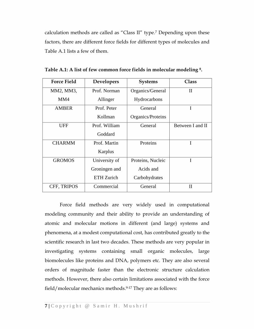
calculation methods are called as “Class II” type.7 Depending upon these
factors, there are different force fields for different types of molecules and
Table A.1 lists a few of them.
Table A.1: A list of few common force fields in molecular modeling 8.
Force Field Developers Systems Class
MM2, MM3,
MM4
Prof. Norman
Allinger
Organics/General
Hydrocarbons
II
AMBER Prof. Peter
Kollman
General
Organics/Proteins
I
UFF Prof. William
Goddard
General Between I and II
CHARMM Prof. Martin
Karplus
Proteins I
GROMOS University of
Groningen and
ETH Zurich
Proteins, Nucleic
Acids and
Carbohydrates
I
CFF, TRIPOS Commercial General II
Force field methods are very widely used in computational
modeling community and their ability to provide an understanding of
atomic and molecular motions in different (and large) systems and
phenomena, at a modest computational cost, has contributed greatly to the
scientific research in last two decades. These methods are very popular in
investigating systems containing small organic molecules, large
biomolecules like proteins and DNA, polymers etc. They are also several
orders of magnitude faster than the electronic structure calculation
methods. However, there also certain limitations associated with the force
field/molecular mechanics methods.9-17 They are as follows:

8 | C o p y r i g h t @ S a m i r H . M u s h r i f
1) Out-of-ordinary/Unusual situation 7, 13, 15, 16: Force field methods are
based on various approximate functional forms and their parameters.
Since the parameters are determined using experimental data, these
methods are empirical. Force field methods perform extremely well when
a lot of information about the system under investigation already exists in
the force field. For molecules that are “exotic” or a little “unusual” and for
which there is little information known, the force field methods may
perform poorly. To summarize, the interpolative force field methods may
lead to serious errors when used for extrapolation.
2) Diverse types of molecules 7, 13, 15, 16: Parameterization of a force field
needs a balance between generality and accuracy. The
generality/transferability of a force field can be improved by including
diverse types of molecules in the parameterization process but with a
given functional form of the energy terms, including additional data may
not help. On the other hand, changing the functional form or using
additional terms, may remove the cancellation of the error effect in the
simpler forms. Most of the force fields are restricted for specific types of
molecules.
3) Chemical reactions 13, 18: While performing force field calculations, the
input consists of (i) types of atoms, (ii) interactions between those atoms
(bonded or non-bonded) and (iii) the geometry. The first two factors are
crucial in assigning an appropriate functional form to each interaction in
the system. The force field calculations are appropriate when the type of
every atom and its types of interactions do not change with changes in
atomic coordinates. However, during the course of a chemical reaction,
covalent bonds are formed and are broken. Hence, a chemical reaction
leads to different energy functions in reactants and products for the same
atom. The electronic structure of the system also changes significantly
thereby changing the type of an atom (e.g. a carbon that was sp3 before the
9 | C o p y r i g h t @ S a m i r H . M u s h r i f
reaction may become sp2 or sp after the reaction and vice-versa). These two
factors in a chemical reaction change the fundamental information on
which the force field energy was calculated and thus the energy will not
remain smooth and continuous during the chemical reaction. Hence force
field calculations fail to model a system in which chemical reactions occur.
The harmonic description of the stretching energy would make it
impossible to find parameter values describing the dissociation of a
molecule.
4) Metal systems 7, 9-11, 14, 17, 19-23: Force field methods are believed to be
difficult, if not impossible, to apply to metal compounds and complexes
and especially to transition metal systems. The bonding in metals is much
different than in organic systems. In the case of metal-ligand complexes,
the metal forms a coordinate bond with the complex while in pure
metallic systems, the bonding may vary with the size of the metal cluster.
Since electronic effects can not be taken into account explicitly in force
field calculations, they need to be taken into account implicitly. The key
reasons for less successful implementation of force field methods to model
metal (including transition metals) complexes and compounds are as
follows:
Varied coordination numbers and geometries: In metal-complexes,
(organic or inorganic) coordination number of a metal is the number of
atoms in the ligand to which the metal is bound and in case of metal
clusters, it is defined as the number of nearest neighbour atoms. Transition
metals may exhibit coordination numbers ranging from 1 to 12. There are
also more than one ways to organize ligand atoms around the central
metal species, giving rise to isomerism. In case of pure metal clusters,
multiple structures, very close in energy, are present. The geometry may
also differ significantly depending upon the physical state of the system
(solid phase/solution/gas phase). Unlike organic compounds, metal
10 | C o p y r i g h t @ S a m i r H . M u s h r i f
coordinated compounds possess a much wider structural flexibility and
hence a variety of structural motifs are observed.22-24 This leads to
difficulty in defining the energy functional forms to describe them. Force
field methods are successfully applied to quite a few specific systems 20, 21,
25-27 and a few generalized approaches28-30 have also been developed to
tackle the problem.23, 31 However, whenever force field methods need to be
applied to a new system, very frequently a significant modification is
required to be performed and the predictive power still remains
questionable.9, 14
Varied oxidation states and electronic structures: Another problem
in using force field methods is that transition metals exhibit multiple
oxidation numbers and electronic states (e.g. palladium has oxidation
states of 0, 1, 2 and 4) and separate parameterization needs to be
performed (similar to carbon with sp, sp2, and sp3 hybridization). The
problem is further magnified due to multitude of transition metal
complexes, thus making the parameterization even more difficult.9, 19, 32, 33
Also in pure metallic systems, the nature of bonding and electronic
structure change as the number of atoms in the metal cluster changes (e.g.
Pd2 has a spin multiplicity of 3, Pd11 has a spin multiplicity of 7 and Pd12
has a spin multiplicity of 5).34
The d-shell electrons 10, 11: In the case of transition metal systems,
the effects due to d-orbital electrons pose further problems in using force
field methods. The structural, spectroscopic and magnetic properties of
transition metal complexes are significantly affected by the d-orbital
electrons. Some significant issues are the Jahn-Teller distortion, s-d orbital
mixing etc. Some efforts have been directed towards tackling these
problems in force field methods and the POS (points on a sphere) model
and the LFMM (ligand field augmented molecular mechanics) model have
garnered relatively more attention.11 However, these modifications are
11 | C o p y r i g h t @ S a m i r H . M u s h r i f
very specific and need significant code writing since they can not be
implemented in standard force field method softwares and to make these
approaches more diversified a lot of parameterization is needed. Another
situation that may hamper the use of these methods is when the system
under investigation contains both, the transition metal complexes and
some routine organic molecules.
A.2.2 Electronic Structure Calculations
To model chemical reactions taking place in a system containing
novel transition metal clusters and complexes and routine organic
compounds, at an atomic level, there is no substitution to the electronic
structure calculation methods. Since it explicitly takes into account the
electronic structure, it also offers an additional advantage of probing and
predicting the bonding and electronic structure changes in the system. The
following sub-sections describe the necessary background material of
electronic structure calculations and give a detailed description of the
methods.
A.2.2.1 Electronic Structure of Atom and Wave-particle duality
An atom consists of electrons, protons and neutrons (Protons and
neutrons are not the most fundamental particles of matter and they are
made up of even smaller particles called quarks. However, these details
are not required and are beyond the scope of this document). Electrically
neutral neutrons and positively charged protons are bound together
forming a positively charged nucleus and the negatively charged electrons
arrange themselves around the nucleus. There exists electromagnetic
interaction amongst these species. The wave-particle duality is known to
exist for a long time to describe matter and energy in physics and
chemistry and an appropriate mathematical form to describe an object
depends upon its mass (and velocity when relativistic effects need to be

12 | C o p y r i g h t @ S a m i r H . M u s h r i f
considered). Heavy objects can be treated as “particles only” and hence
can be modelled using classical Newtonian mechanics. However, the
borderline mass for Newtonian mechanics is the mass of a proton (and the
velocity as a fraction of the velocity of light, to neglect relativistic effects).
Electrons are a few orders of magnitude lighter than the neutrons and
protons (and hence the nucleus) and hence they display both wave and
particle like characteristics. The famous double slit-experiment was the first
experimental proof of electrons behaving like a wave. Given the wave like
behaviour of electrons, it is not possible to mathematically treat electrons
using classical Newtonian mechanics and hence they need a special
treatment, i.e. quantum mechanics.
A.2.2.2 Postulates of Quantum Mechanics
Quantum mechanics is nothing but a set of underlying principles
that can describe some of the most fundamental aspects of matter at a sub-
atomic level. The postulates of quantum mechanics are as follows: 7
1. Associated with any particle (like an electron) moving in a force
field (like the electromagnetic forces exerted on an electron due to the
presence of other electrons and nuclei) is a wave function which
determines everything that can be known about the particle.
2. With every physical observable there is an associated operator,
which when operating upon the wavefunction associated with a definite
value of that observable will yield that value times the wavefunction
n n nQ q .
3. Any operator associated with a physically measurable property will
be Hermitian **
a b a bQ dr Q dr .
4. The set of eigenfunctions of the operator will form a complete set of
linearly independent functions and j j j j jQ q c .

13 | C o p y r i g h t @ S a m i r H . M u s h r i f
5. For a system described by a given wavefunction, the expectation
value of any property can be found by performing the expectation value
integral with respect to that wavefunction *q Q dr .
A.2.2.3 Schrödinger Equation
The Schrödinger equation,35 which is a second order partial
differential equation, is the most important equation in quantum
mechanics and can describe the spatial and temporal evolution of the
wavefunction of a particle in a given potential. It is given as,
, ,H r t i r tt
(A.9)
where is the reduced Planck’s constant, is the wavefunction and H
is the Hamiltonian operator which is given as follows:
2
2
2H U r
m
(A.10)
The first term in the Hamiltonian operator is the kinetic energy operator
and the second term is the potential energy operator. Since equation (A.9)
is a partial differential equation, if the separation of variables method is
used, the wavefunction can be separated into spatial and temporal part as
,r t r f t (A.11)
Inserting equation (A.11) into equation (A.9) gives
1 1 dH r i f t
r f t dt
(A.12)
The left hand side of equation (A.12) depends only on space while the
right hand side depends only on time. Since these two are completely
independent variables, equation (A.12) can only be true when both the
sides of the equation are constant, i.e.
1; H r E H r E r
r
(A.13)

14 | C o p y r i g h t @ S a m i r H . M u s h r i f
E is a constant in equation (A.13). According to postulate number 2 of
quantum mechanics, with every physical observable there is an associated
operator. Since the Hamiltonian is an energy operator, it is intuitive that
the constant E is nothing but the energy of the system. The solution of the
time dependant right hand side part of equation (A.12) can be given as
iEtf t e and inserting this solution in equation (A.11) gives,
, iEtr t r e (A.14)
Thus the wavefunction is written as a function with amplitude r and
phase iEte . Inserting equation (A.14) into equation (A.9) gives the time
independent Schrödinger equation as
H r E r (A.15)
and the time dependence can be written as a product of the time
independent function and the phase factor. The phase factor is usually
neglected for time-independent problems.
A nucleus is much heavier than electrons and this large mass
difference also indicates that its velocity is much smaller than that of the
electrons. Hence nuclei exhibit small quantum effects and can be treated
classically. The electrons can adjust instantaneously to any change in the
nuclear coordinates. If we write the time-independent Schrödinger
equation for a system where n denotes nuclei and e denotes electrons and
the nuclear coordinates are denoted as nR and the electronic coordinates
are denoted as er then,
, ,sys sys e n sys sys e nH r R E r R (A.16)
where
,sys n e ee e en e n nn n n eH T T V r V r R V R T H (A.17)
T denotes the kinetic energy operator and V denotes the potential energy
operator (columbic interactions between electron-electron, electron-
15 | C o p y r i g h t @ S a m i r H . M u s h r i f
nucleus and nucleus-nucleus). The total wavefunction of the system
depends on the coordinates and velocities of the electrons and the nuclei.
However, due to the separation of time scales between the electronic and
nuclear motion (nuclei moving much slower than the electrons) it can be
assumed that the nuclei are almost stationary with respect to the electrons.
If the total wavefunction of the system is written as
,sys e e n n nr R R (A.18)
then the Schrödinger equation in a static arrangement of nuclei can be
written as
, ,e e e n e e e nH r R E r R (A.19)
Here the energy eE and the wavefunction e depend only on the nuclear
coordinates and not on nuclear velocities. The total energy of the system
then can be computed from the following equation.
n e n n sys n nT E R E R (A.20)
The energy eE is often called the adiabatic contribution to the energy of
the system and it is shown that the non-adiabatic contributions contribute
very little to the energy. The error in hydrogen molecule is of the order of
10-4 a.u. and as the molecule gets bigger, the nuclei become heavier and
thus the error decreases.7 Thus, with the separation of nuclear and
electronic motion, we can compute the energy eE as a function of different
nuclear coordinates. This way of computing the energy using e provides
a potential energy surface on which the nuclei move. The separation of
electronic and nuclear motion in a system, as described above, is called as
the Born-Oppenheimer approximation. Most of the electronic structure
calculations are performed using this approximation (i.e. using equation
A.19 instead of equation A.16) and all the electronic structure calculation
methods described henceforth in this will be using the Born-Oppenheimer
approximation.
16 | C o p y r i g h t @ S a m i r H . M u s h r i f
A.2.2.4 Solution for Hydrogen atom and Approximate Solution for Helium
The hydrogen atom is the simplest system on which electronic level
calculations can be performed by solving the Schrödinger equation. For
the hydrogen atom, with one electron and a nucleus of charge +1, the time
independent Schrödinger equation can be written as,
2
2
2U r r E r
m
(A.21)
where r is the distance of the electron from the nucleus and the potential
energy operator takes into account the columbic interaction between the
electron and the nucleus 1U r r . The analytical solution for the
wavefunction in spherical coordinates is given as,7
3
2 2 1
1 ,
0
1 !2, , . ,
2 1 !
l l
nlm n l l m
n lr e L Y
na n n
(A.22)
where n, l and m are the principal, azimuthal and magnetic quantum
numbers, 0a is the Bohr radius, 02r na , 2 1
1
l
n lL
are Laguerre
polynomials and lmY are spherical harmonics.
Once the wavefunction is determined, the square of the
wavefunction at any point gives the probability of finding an electron at
that point. Hence,
1d (A.23)
The physical quantity that is associated with the Hamiltonian operator H
is the energy and is given as
H dE H d H
d
(A.24)
It is a customary to write the integrals using a “Bra-ket” notation, as
shown in equation (A.24).

17 | C o p y r i g h t @ S a m i r H . M u s h r i f
The solution of Schrödinger equation for a system containing more
than one electron is more complicated since no analytical solution exists.
An approximate solution needs to be determined even for the helium
atom which contains two electrons and a nucleus. The Schrödinger
equation for this atom can be written as 8
1 2
2 2
1 2 1 2
1 2 12
1 2 1 2 1 2 1 2
12
1 1 1,
2 2
1, , ,
h h
Z Z
r r r
h h H Er
r r
r r r r r r
(A.25)
where Z denotes the charge on the nucleus, subscripts 1 and 2 represent
electrons 1 and 2 and 1 2 and r r represent their positions in space. If we
assume that the two electrons in the atom interact with the nucleus but do
not interact with each other, i.e. 1 2H h h , then equation (A.25) becomes
separable and an exact solution of the individual electron’s wavefunction
can be obtained. The two separate equations are
1 1 1 1 1 1 2 2 2 2 2 2 and h E h E r r r r (A.26)
and the total wavefunction then can be assumed as a product of
individual wave functions 1 2 1 1 2 2, r r r r . The total energy of the
helium atom with non-interacting electrons then can be given as
1 2E E E . To include the correction for repulsion between the two
electrons in helium atom, an additional term can be defined as,
1 2 2 2 1 1
12 12
1 1 and eff effU d U d
r r (A.27)
Since 1 and 2 are known from the non-interacting system, integrals in
equation (A.27) can be evaluated. Using equation (A.27), the effective
Hamiltonian that takes into account the electron-electron repulsion can be
defined as
18 | C o p y r i g h t @ S a m i r H . M u s h r i f
1 1 1 2 2 2
1 1 1 1 2 2 2 2 1 2 1 2
and
and , , ,
eff eff eff eff
eff eff
H h U H h U
H E H E E E
(A.28)
Thus the total energy of the system with interacting electrons, E can be
calculated as
1 2 1 2 1 2
12
1 2 1 2
12 12
1 2 1 2 1 2 1 2
12True Hamiltonian for He
1 2 1 2 12
12
1 2 12
2
1 1
1
1
eff effE E H H h hr
H Hr r
Hr
E d E Jr
E E E J
(A.29)
12J is called as the Coulomb integral. It can be seen that the exact solution
of hydrogen atom plays an important role in calculating an approximate
solution for the helium atom.
Both the electrons in helium are in the 1s orbital and it means that
they have the same principal, azimuthal and magnetic quantum numbers.
However, they differ in the spin since one has a 1 2 spin and the other
has 1 2 spin. In the above discussion, the total wavefunction of the
helium atom is written as the product of individual electron
wavefunctions as
1 2 1 1 2 2, 1 1 1 2s s r r r r (A.30)
where the wavefunctions/orbitals 1 and 1s s differ in spin. Pauli’s
exclusion principle states that, for two electrons, the total wavefunction is
antisymmetric 1 2 2 1, , r r r r . However, if is defined as in
equation (A.30) and we exchange electrons 1 and 2, we get
1 2 2 1
1 2 2 1
, 1 1 1 2 and , 1 2 1 1
, ,
s s s s
r r r r
r r r r (A.31)

19 | C o p y r i g h t @ S a m i r H . M u s h r i f
Equation (A.31) does not obey Pauli’s exclusion principle. Hence the
representation of the total wavefunction needs to be changed. A correct
representation would be
1 2
1, 1 1 1 2 1 2 1 1
2
1 1 1 11 =
1 2 1 22
s s s s
s s
s s
r r
(A.32)
The determinant in equation (A.32) is called as Slater determinant. If the
correct representation of the total wavefunction is put in equation (A.29),
we get
1 2 1 2 1 2
12 12
12True Hamiltonian for He
12 12
Coulomb Integral
2 1
1 1 1 1 1 2 1 2 1 1 1 1 1 2 1 2 1 1
2
1 1 1 1 1 1 1 2 1 1 1 2 1 2 1 1 1 2 1 1
2 2
eff effE E H H h h Hr r
H s s s s s s s sr
E s s s s s s s sr r
12 12
Exchange Integral
12 12
1 2 12 12
1 1 1 1 - 1 1 1 2 1 2 1 1 1 2 1 1 1 1 1 2
2 2
s s s s s s s sr r
E J K
E E E J K
(A.33)
A.2.2.5 Linear Combination of Atomic Orbitals (LCAO)
The discussion in the above section is limited to Helium, containing
only two electrons; however, any realistic system will be a polyelectronic
system. Any system consists of molecules and when more than one atoms
form a molecule (by forming electron sharing and non electron sharing
bonds), their electronic structure gets modified. For example, when two H
atoms form a covalent bond to make an H2 molecule, the electronic
20 | C o p y r i g h t @ S a m i r H . M u s h r i f
structure is different than that of an individual hydrogen atom. According
to the valence bond theory, the individual orbitals of two atoms overlap
and the shared electrons are localized in the overlapped region (the bond)
between the two atoms. However, in electronic structure computations,
the molecular orbital theory is used. According to this theory, the
electrons are not assigned to individual bonds and are considered to
arrange themselves around the molecule, under the influence of the
nuclei. Similar to orbitals in an atom, every molecule is considered to have
a set of molecular orbitals and these molecular orbitals (wavefunction) are
a mathematical construct of the individual atomic orbitals. Molecular
orbitals are expressed as a linear combination of atomic orbitals (LCAO),7
as if each atom were on its own.
1 1 2 2 3 3 ....... n nc c c c (A.34)
where is the molecular orbital, i is an atomic orbital and ic is the
coefficient associated with the atomic orbital i . To make sure that the
orbitals follow the antisymmetric constraint, they are expressed as Slater
determinants (similar to equation A.32). If there are N electrons in the
system with spin orbitals 1 2, , , N then the total wavefunction is given
as,
1 2
1 2
1 2
1 2
1 1 1
2 2 211,2, ,
!
= 1 2
N
N
N
N
NN
N N N
N
(A.35)
Since in a polyelectronic system, it is not possible to obtain analytical
solution, assuming non-interacting electrons (the way it is obtained in the
case of Helium), the atomic orbitals are expressed in the form of basis
functions. A basis function can be of any type; exponential, Gaussian,

21 | C o p y r i g h t @ S a m i r H . M u s h r i f
polynomial, cube function, planewaves, to name a few. Though these
basis functions need not be an analytical solution to an atomic Schrödinger
equation, they should properly describe the physics of the problem and
these functions go to zero when the distance between the nuclei and the
electron becomes too large. The two types of basis functions commonly
used to construct atomic orbitals are the Slater type orbital and the
Gaussian type orbital. The functional form of the Slater type orbitals is as
follows8
1
, , , ,, , , n r
n l m l mr NY r e
(A.36)
where N is a normalization constant, is a constant related to the effective
charge of the nucleus and ,l mY are spherical harmonic functions. The
Gaussian type orbitals are given as follows8
22 2
, , , ,, , , n l r
n l m l mr NY r e
(A.37)
The Slater type basis functions are superior to the Gaussian type basis
function since less number of Slater orbitals are required to get a given
accuracy and the physics of the system is better described using the Slater
type orbitals.7
The minimum number of basis functions that are needed to
describe any system is that which can just accommodate the number of
electrons present in the system. For ex. two sets of s functions (1s and 2s)
and a set of p functions (2px, 2py and 2pz) are required to describe the first
row elements in the periodic table. Increased accuracy can be obtained
using a larger number of basis functions. A detailed overview on different
types of basis functions is beyond the scope of this document and hence
not discussed here. The basis functions used in condensed phase and
periodic systems are planewaves and the pertaining details will be
discussed in section A.2.4.

22 | C o p y r i g h t @ S a m i r H . M u s h r i f
A.2.2.6 Hartree-Fock Calculations
While performing electronic structure calculations in a
polyelectronic system, we are aiming to calculate the molecular orbitals
(and the energy). Once the type and numbers of basis function are
decided, the molecular orbitals are formed as a linear combination of
atomic orbitals, as in equation (A.34), and the wavefunction is expressed
in the form of Slater determinant, as in equation (A.35). Since there is no
“exact” wavefunction, we need to determine the coefficients of equation
(A.34) which will give the best possible solution. The variational principle
is used to calculate these coefficients and ultimately the wavefunction. It
states that the energy calculated from an approximate wavefunction will
always be bigger than the “true” energy of the system.7 This implies that
the closer the approximate wavefunction to the actual solution, lower will
be the energy of the system. Hence to obtain the best possible
wavefunction, we need to determine the set of coefficients that will result
in the minimum energy of the system i.e. the electronic energy of the
system is minimized with respect to the coefficients. The numerical
procedure is as follows.
If there is an N electron system for which the Hamiltonian is given
as
21 1
2
N N N N
i i i ji i j
i ij
ZH
r r r r
h g
(A.38)
and the wave function is expressed as a Slater determinant, as in equation
(A.35) , then the energy is given as,

23 | C o p y r i g h t @ S a m i r H . M u s h r i f
1 2 1 2
1 2 1 2
2
= 1 2 1 2
1 2 1 2
=2
N N N
i ij
i i j
N
N i N
i
N N
N ij N
i j
N N N Ni
i i i i ij ij
i i i ji
E h g
N h N
N g N
ZJ K
r
(A.39)
where
12 1 2 1 2 12 1 2 2 1
12 12
1 11 2 1 2 and 1 2 1 2J K
r r
(A.40)
If every orbital is doubly occupied then,
,
2 2n n
ii ij ij
i i j
H h J K (A.41)
Varying the electronic energy as a function of orbitals and equating it to
zero we get,
, ,
2 2 2
0 2
n n n
ii ij ij ij i j ij
i i j i j
n n
i j j i ij j
j ji
h J K
h J K
(A.42)
where ij are the Lagrange multipliers that are introduced because the
minimization of the energy needs to be performed under the constraint
that the molecular orbitals remain orthogonal and normalized.
Since the wavefunction is a determinant, the matrix ij can be
brought into diagonal form as 0 and ij ii i ,
2n
i j j i i i i i
j
h J K
F (A.43)
Expressing i
M
ic
we get,

24 | C o p y r i g h t @ S a m i r H . M u s h r i f
M M
i i i ic c
F (A.44)
where ijc are the coefficients and M is the number of basis functions.
Multiplying equation (A.44) by a specific basis function and integrating
gives the following equation
and |F S
Fc Sc
F (A.45)
where F is called as the Fock Matrix and S is called as the overlap matrix.
Equation (A.45) is an eigenvalue problem and the Fock matrix needs to be
diagonalized to get the coefficients of the molecular orbitals. But it has to
be noted that the Fock matrix can only be calculated if the coefficients are
known. Hence, the Hartree-Fock procedure to perform electronic level
calculations starts with an initial guess for the coefficients, then calculating
the Fock matrix and then recalculating the new set of coefficients by
diagonalizing the Fock matrix. The procedure is repeated till the
coefficients used to form the Fock matrix are the same to those emanating
from the diagonalization of the Fock matrix. The convergence on the
coefficients implies that the system is at the minimum energy.
A.2.2.7 Semi-empirical methods
The electronic structure calculation methods, like the Hartree-Fock
method described above, are computationally very expensive and a
significant amount of computational effort is needed to calculate and
manipulate the integrals that are calculated in the process. Hence, to
reduce the computational cost of electronic structure calculations, some
approximations are made to these integrals, particularly to the two-
electron, multicentre integrals. These integrals are either neglected or are
parameterized using empirical data. Such methods are called as semi-

25 | C o p y r i g h t @ S a m i r H . M u s h r i f
empirical methods.36 Some common semi-empirical methods are Zero-
differential overlap (ZDO), Complete neglect of differential overlap
(CNDO), Intermediate neglect of differential overlap (INDO), Neglect of
diatomic differential overlap (NDDO), Modified neglect of diatomic
overlap (MNDO), Austin model-1 (AM1), Parametric model-3 (PM3) etc.36
A detailed discussion of all these methods is not included here. However,
these semi-empirical methods share a limitation of force field methods,
i.e., their performance on unknown species. The extent of this limitation is
not as severe as in the case of force field calculations though. Most of these
methods also use the minimal basis function only.
A.2.2.8 Post Hartree-Fock
The electronic structure calculations are performed in the Hartree-
Fock procedure by selecting the type and number of basis functions,
forming a Slater determinant and then obtaining the coefficients in an
iterative fashion, as explained in the previous section. The accuracy of
these calculations can be improved (or the energy of the system can be
further lowered) by increasing the number of basis functions used. The
Hartree-Fock wavefunction can provide 99% accuracy in calculating the
“true” energy of the system and hence suffices the purpose in a lot of
cases. However, in certain situations, this 1% difference becomes very
crucial to describe correctly the physics of the system. In order to further
improve the accuracy of electronic structure calculation methods beyond
the Hartree-Fock procedure, it is required to identify the root cause of this
slight inaccuracy. Assuming that a sufficiently large basis set is used, the
other possible source of error is due to electron-electron interaction
treatment in the Hartree-Fock procedure. Though the electron-electron
interaction is taken into account, as can be seen in equation (A.39), it has to
be noted that each electron in the Hartree-Fock procedure sees an average

26 | C o p y r i g h t @ S a m i r H . M u s h r i f
field of all other electrons and the motion of each and every electron is not
correlated. In other words, an electron does not see each and every other
electron as individual point charge so as to avoid it as much as possible. It
also does not allow electrons to cross each other. Hence, any method that
can improve the electron correlation this way will definitely lead to a
lower energy of the system than that calculated using the Hartree Fock
procedure. These methods are called as electron correlation methods and
the electron correlation energy is the difference between the “true” energy
of the system and the energy calculated using the Hartree Fock procedure.
One of the ways to further improve the electron correlation effects
in electronic structure calculations is to include additional (Slater)
determinants. Addition of determinants in the mathematical formulation
can also be seen physically as addition of some unoccupied/virtual
orbitals to the system, something very similar to addition of excited state
orbitals to the ground state orbitals of the system.
0 1 1 2 2HF
corrrelation c c c (A.46)
where HF is the single determinant wavefunction obtained using the
Hartree-Fock procedure and i are the additional determinants. There are
3 main methods that are used to take into account electron correlation
effects, viz., Configuration Interaction (CI)37, Coupled Cluster (CC)38 and
Møller-Plesset (MP)39 and they differ in ways to calculate the coefficients
in equation (A.46). Further details of these methods are beyond the scope
of this document and hence not provided here.
A.2.3 Density Functional Theory (DFT)
The previous section described the electronic structure calculation
methods (Hartree-Fock, Semi-empirical and Post-Hartree-Fock) based on
the multielectron wavefunction of the system. However, there exists one
more theoretical approach to perform electronic structure calculations and

27 | C o p y r i g h t @ S a m i r H . M u s h r i f
it is called as density functional theory. As the name suggests, the energy
of the system containing N electrons that repel each other, get attracted to
the nuclei by Columbic interaction and follow Pauli’s exclusion principle
is calculated using the density of electrons instead of the wavefunction.
The following sections describe the mathematical formulation of the
density functional theory and the necessary details.
A.2.3.1 Origin and formulation of DFT
The Schrödinger wave equation for an N electron system is given
as
21 1
2
N N N N
i i j iij i
ZE
r r
r
(A.47)
and, as mentioned before, the ground state electronic density of the
system can be calculated as
1 1 1 1 1 12 , ,2, , , , 2, ,r N dx d dN r x N r x N (A.48)
Equations (A.47) and (A.48) show that for a given potential r , it is
possible to compute the ground state density r , via the electronic
wavefunction . However, Hohenberg and Kohn40 showed that there
exists an inverse mapping with which it is possible to obtain an external
potential, if the ground state density is provided. In their seminal paper,40
they also showed that this inverse mapping can be used to calculate the
ground state energy of a multielectron system using the variational
principle, without having to resort to calculate the wavefunction. If the
wave function is expressed as
(A.49)
then since , the wavefunction can be written as

28 | C o p y r i g h t @ S a m i r H . M u s h r i f
(A.50)
Using the variational principle, the energy of the system can be calculated
as,
min min
min ee
E H H
T V
(A.51)
where 2 1
= , and 2
ee
ee
ZT V
r r
.
Equation (A.51) can be separated as,
3
E min
min
eeT V
F
d r r r F
(A.52)
The energy is thus minimized over the density and not over the
wavefunction. However, in equation (A.52), the functional form of F
is unknown.
The inverse mapping of density on potential is also valid for a
system of non-interaction electrons and Thomas-Fermi,41, 42 even before
the Hohenberg-Kohn theorem,40 provided a way to calculate the energy of
such a non-interacting system by replacing the wavefunction with electron
density as follows. For a non-interacting system,
23 3
1 1
23 3
1 1
2
2
N N
i i i i
i i
N N
i i
i i
E d r r r d r r r r
d r r r d r r r
(A.53)
As shown in equation (A.53), Thomas-Fermi just replaced the
wavefunction with the electron density. They also showed that the kinetic
energy part of a homogeneous electron gas is given as,

29 | C o p y r i g h t @ S a m i r H . M u s h r i f
2 3
2 3 5 333
10sT d r r (A.54)
Hence according to Thomas-Fermi approach the energy of the non-
interacting system can be given in terms of the electron density as,
2 3
2 3 5 3 3
1
33
10
N
i
E d r r d r r r
(A.55)
This Thomas-Fermi approach of calculating the kinetic energy part of the
non-interacting system of electrons is used to develop a scheme to
evaluate the functional F (for a system with interacting electrons) and
the details are provided in the following section.
A.2.3.2 Kohn-Sham formulation
To calculate the unknown functional F consisting of the
electronic kinetic energy part and the electron-electron interaction part,
Kohn and Sham43 came up with a scheme which calculates the total
energy of the system using a combination of the density functional theory
and orbital/wavefunction approach. A detailed description is as follows.
Kohn-Sham introduced a non-interacting system for which the
Hamiltonian can be given as
21
2ks KSh r (A.56)
If an orbital corresponding to the above Hamiltonian (usually referred as
Kohn-Sham orbitals) is given in the form of a determinant as
KS 1 2 3 1 2 3 ... N N (A.57)
then the Schrödinger equation will be
KS KS KS KSh E (A.58)
In the Kohn-Sham formulation, the potential KS r is defined in such a
way that the electron density calculated using the Kohn-Sham orbitals KS
is equivalent to the exact density of the electron-interacting system with
30 | C o p y r i g h t @ S a m i r H . M u s h r i f
the actual potential r . Using the Kohn-Sham orbitals, the kinetic
energy of the non-interacting system can be given as
S KS KST T (A.59)
From equations (A.56-A.59), with the actual wavefunction of the system as
, the ground state electronic energy of the system can be given as,
3
3 3 31
2
ee ee
K
S
K s ee
XC
E T V T d r r r V
T
r rT d r r r d rd r
r r
U
T T V U
E
(A.60)
where sT is the kinetic energy which can be calculated using the Kohn-
Sham orbitals. XCE is the only unknown function in the above
equation that needs to be approximated. It accounts for less than 10% of
the total energy.8
It is possible to calculate the total ground state energy of the
interacting system using the following steps:
(i) Define the Kohn-Sham non-interacting system
(ii) Calculate the density and kinetic energy of the system and
(iii) Calculate the ground state energy
However, it is only possible if the Kohn-Sham potential KS r is known.
The methodology to determine the potential is as follows.
From equations (A.56) and (A.58) we get
3minKS S KSE T d r r r
(A.61)
where 0 0KS SKS
E T
(A.62)

31 | C o p y r i g h t @ S a m i r H . M u s h r i f
From equation (A.60), the actual ground state energy of the system is
given as
3min S XCE T d r r r U E
(A.63)
where 30 0S XCrT EE
r d rr r
(A.64)
Combining equations (A.62) and (A.64), the Kohn-Sham potential can be
obtained as
3 XC
KS
r Er r d r
r r
(A.65)
If an approximate functional for XCE is known, the Kohn-Sham non-
interacting system can be solved to obtain the Kohn-Sham orbitals KS
and the density . Using this information the total energy of the system
can be calculated using equation (A.63). However, since the Kohn-Sham
potential depends on density the above equations need to be solved
iteratively.
To use the Kohn-Sham Density Functional theory, it is needed to
have an appropriate functional form for XCE and the following section
describes the approaches to obtain it.
A.2.3.3 Local density approximation and Generalized Gradient Approximation
From equation (A.60) it can be seen that the XCE term accounts for
(i) the difference between the actual/exact electronic kinetic energy of the
system and the Kohn-Sham non-interacting electronic kinetic energy
K sT T and (ii) the difference between the exact electron-electron
interaction energy and U (analogous to the Coulomb integral term J
in the Hartree-Fock method, as shown in equation A.39). In other words, it
accounts for the exchange-correlation energy XC X CE E E . The two

32 | C o p y r i g h t @ S a m i r H . M u s h r i f
common approximations for the functional XCE are the local density
approximation (LDA) and the generalized gradient approximation
(GGA).44
As described in section A.2.3.1, the energy of non-interacting,
homogeneous electron gas is given using equation (A.55) as
2 3
2 3 5 3 333
10d r r d r r r . However, it only takes into account
the kinetic energy part and the electron-nuclear interactions and neglects
the electron-electron interaction energy. A next step in this procedure is to
take into account the Coulomb interaction energy given by the term U ,
thus extending the Thomas-Fermi energy to
2 3
2 3 5 3 3 3 33 13
10 2TF
r rE d r r d r r r d rd r
r r
(A.66)
Equation (A.66) is a step ahead from the completely non-interacting
system but it still does not take into account the exchange and correlation
energy. Dirac 45 developed an exchange energy formula for the uniform
electron gas as
1 3
4 3
1 31 3
3 3
4
3 3
4
X
X
E r dr
Er
(A.67)
Since,
XC CXXC X C
E EEE E E
(A.68)
Ceperley and Alder 46 determined the exact values of CE
using numerical
simulations and Vosko et al.47 interpolated those values to obtain an
analytical function for the same. This analytical expression is given in the

33 | C o p y r i g h t @ S a m i r H . M u s h r i f
spin-dependant form (if the electrons have spins and , then the total
electron density is given as ) as
2 4 4
2
2
, ,
,0 1 ,1 ,00
Cs c s
c s a s c s c s
Er r
fr r r r f
f
(A.69)
where
4 3 4 3
2 1 3
2 21
2 2
/ 2 20 0 10
2 2 20 0
11 1 2
2
2 1
2 4ln tan
24
2 2 4ln tan
24
c a
f
x b c b
x bx c x bc bx A
x x b xbx c b
x bx c x bx c x bc b
(A.70)
sx r and 0, , ,A x b c are fitting constants. sr is the effective volume
containing an electron and the spin polarization is given as
. Thus, for a uniform electron gas, the total energy of
the system can be given as,
2 32 3 5 3 3
1 3
3 3 4 3 3
3
33
10
1 3 3
2 4
+
TF
C
E d r r d r r r
r rd rd r r d r
r r
Er d r
(A.71)
In the Kohn-Sham density functional theory approach (as discussed in
section A.2.3.2) , when the exchange correlation term XCE in equation
(A.60) is assumed to be equal to that of the uniform electron gas

34 | C o p y r i g h t @ S a m i r H . M u s h r i f
1 3
4 3 3 33 3+
4
CXC
EE r d r r d r
as shown in equation
(A.69), it is referred to as Local Density Approximation or LDA.
The Generalized gradient approximation or GGA is an
improvement over the LDA since it implements the gradient correction as
3 g ,GGA
XCE d r (A.72)
For the GGA to be practically useful, it is again important that it has an
analytical form like LDA. Different popular formats of the GGA48-54 are
used in the electronic structure calculations, but only the Perdew-Burke-
Ernzerhof approximation52 will be discussed here.
Similar to the LDA, the XCE term is again separated into the
exchange and correlation parts in GGA and in the Perdew-Burke-
Ernzerhof approximation,52 the correlation term is given as
3, , , GGA
C C s sE r H r t d r (A.73)
where t is the dimensionless density gradient given as 2 st k ,
is the scaling factor given as 2 3 2 3
1 1 2
and
1 3
2 2 24 3sk me . The functional form of H in equation (A.73)
is given as
2
2 2 2 3 2
2 2 4
0.066725 10.031091 ln 1
0.031091 1
AtH e me t
At A t
(A.75)
where 1
3 2 2 20.066725exp 0.031091 1
0.031091CA e me
The exchange energy term for this GGA approximation is defined as
3GGA
X x XE F s d r (A.76)
where s is another type of reduced density gradient given as
0.5
2 2 1.2277sr me t and the functional form of XF is as follows.

35 | C o p y r i g h t @ S a m i r H . M u s h r i f
2
0.8041 0.804
0.219511
0.804
XF ss
(A.77)
A.2.4 Planewave-pseudopotential Methods
The above sections describe the multielectron system’s electronic
structure calculations using the Kohn-Sham density functional theory
within the framework of Born-Oppenheimer approximation. Even though
the density functional theory takes into account the electron correlation at
the computational cost of Hartree-Fock theory, it is computationally still a
difficult task to apply this method to an extended system like crystals or
bulk soft matter. The solution to this problem is to define a tractable size
of system, which when repeated periodically in all spatial directions will
represent the bulk i.e. to apply periodic boundary conditions to the cell
containing a set of atoms/molecules. If the cell is defined by vectors 1a , 2a
and 3a , then its volume is given as 1 2 3 a a a . General lattice vectors
are integer multiples of these vectors as
1 1 2 2 3 3L N N N a a a (A.78)
A particular atomic arrangement which is repeated periodically, to mimic
the actual system of interest, can reduce the computational cost of the
calculations since the computations are restricted to the lattice. However,
in such an arrangement the effective potential also has a periodicity as
eff effr L r (A.79)
The resultant electron density will also be periodic. Given the periodic
nature, the potential can be expanded as a Fourier series as 55
31 where iGr iGr
eff eff eff eff
G
r G e G r e d r
(A.80)
where the vector G forms the lattice in the reciprocal space which is
generated by the primitive vectors 1b , 2b and 3b in such a way that

36 | C o p y r i g h t @ S a m i r H . M u s h r i f
2i j ij a b , ij being the Kronecker delta. Thus, the volume of the
primitive cell in the reciprocal space is given as 3
1 2 3 2 b b b .
Bloch’s theorem56 states that if r is a periodic potential
r L r , then the wavefunction of a one electron Hamiltonian of
the form 21
2r
is given as planewave times a function with the
same periodicity as the potential. Mathematically it can be written as
.ik r
k kr e u r where k k
u r u r L (A.81)
Alternatively the Bloch’s theorem can be written as55
ik r
k kr L e r (A.82)
It also has to be noted that planewaves are the exact orbitals for
homogeneous electron gas.44 Since the function k
u r is periodic, it can be
expanded as a set of planewaves as55
1 k iG r
GkG
u r c e (A.83)
Combining equations (A.81) and (A.83) we get,
1 i G k rk
GkG
r c e
(A.84)
where k
Gc are complex numbers. While performing electronic structure
calculations of a system with periodic boundary conditions (periodic
potential) using the Kohn-Sham implementation of density functional
theory and planewaves as basis functions, k
r can be seen as the Kohn-
Sham orbitals. In that case the Kohn-Sham density functional theory
equations can be rewritten as
21
2eff k k k
r r r
(A.85)

37 | C o p y r i g h t @ S a m i r H . M u s h r i f
where eff r accounts for nucleus-electron and electron-electron
interactions and the electron density is given as
2 3
32
2Fk k
r r E d k
(A.86)
Factor 2 in the above equation is to take into account both the electron
spins and is the step function which 1 for positive and 0 for negative
function arguments. The integration in equation (A.86) is over the
Brillouin zone (primitive cell in the reciprocal space).
As explained above, using the Bloch’s theorem, a problem of an
extended system with an extended number of electrons is transformed
into a problem within a small periodic cell. This improvement may not be
very satisfactory if the integration in equation (A.86) needs to be
performed at each and every point in the reciprocal space or the k-space
since there are infinite numbers of k-points. However since the electronic
wavefunction at k-points close to each other will be very similar, it is
possible to replace the above integral as a discrete sum over limited
number of k-points.
2 3
3
int
1
2F kk k
k po s
r E d k fN
(A.87)
The error due to this approximation can be minimized by using large
number of k-points.57 Usually it is practised to converge the energy of the
system with respect to the number of k-points in the calculation. However,
as the size of the simulation cell in real space gets larger the size of the
reciprocal space cell becomes smaller. This implies that as the simulation
cell in real space becomes bigger, the k-space and hence the number of k-
points becomes smaller. If the simulation cell is large enough then a single
k-point (often referred as Г-point) is also good enough for the calculation
purpose.
38 | C o p y r i g h t @ S a m i r H . M u s h r i f
A finite number of planewaves are required to perform the
computations. Since the accuracy of the Kohn-Sham potential is
dependant on the accuracy of basis set used for Kohn-Sham orbitals, it is
apparent that a larger basis set would result in a more accurate Kohn-
Sham potential. If plane waves are the basis set then the Kohn-Sham
potential needs to be converged with respect to the number of
planewaves. From equation (A.84), it can be seen that a higher modulus of
G would result in higher number of planewaves. Hence, a limit is placed
in the calculations where the G vectors with a kinetic energy lower than
the specified cut-off are only considered for a calculation.
22
2cutG E
m (A.88)
The precision of the planewave implementation of Kohn-Sham density
functional theory approach is thus dependant on the parameter cutE , as
per equation (A.88). Some of the advantages and disadvantages of using
planewaves as basis functions are
Planewaves are orthonormal and energy independent.
Planewaves are not biased to any particular atom. Hence the entire
space is treated on an equal footing and hence does not cause the basis
set superposition error (due to overlap of individual atom’s basis set)
The conversion between real and reciprocal space representations can
be efficiently performed using Fast-Fourier transform algorithms and
hence the computational cost can be decreased by performing the
calculations in the reciprocal space.
However, it can not take advantage of the vacuum space in the
simulation cell by avoiding having a basis set in that region.
Since the planewaves are independent of the positions of atoms,
Hellman-Feynman theorem can be used to compute the forces15,
thereby reducing the computational cost. In other words, if a basis set
39 | C o p y r i g h t @ S a m i r H . M u s h r i f
is dependant on the nuclear coordinates, then while calculating the
forces the derivatives of the coefficients (with respect to nuclear
coordinates) associated with the basis set also need to be computed.
However if the basis set is independent, the variationally minimized
coefficients can be used, as it they are, to compute the forces.
i i j j
i j
i j i j
i jHellman Feynmann n n
c H cE H
c cR R R
(A.89)
The valence wavefunctions are nodal in the core region of the atom
(Pauli’s exclusion principle) and hence a large number of planewaves
are needed to represent these large oscillations.
For a practical application of planewaves approach, a solution to
the nodal structure of valence wavefunctions problem needs to be identified.
The solution is to use the frozen core approximation i.e. to treat the core
electrons and the nucleus as a pseudocore. The consequence is that the
electron-nuclear potential will also have to replaced by a pseudopotential.
Since this pseudopotential eradicates the core electrons from the system, it
is very important that the pseudopotential takes into account the electron-
nucleus interaction (as if shielded by the core electrons) and the electron-
electron interaction (the classical Columbic and exchange-correlation
interaction between the valence and core electrons). Hence the
pseudopotential is angular momentum dependant as well. Due to this
pseudopotential, the all electron wave function also gets replaced by the
pseudo-wavefunction. Outside a certain cut-off radius the pseudopotential
matches the true potential of the system and the pseudo-wavefunction
matches the true wavefunction of the system (cf. Fig. A.3).
Additionally, it is worth noting that the contribution of core
electrons to chemical bonding is negligible and only the valence electrons
play a significant part in it. The core electrons play an important part in

40 | C o p y r i g h t @ S a m i r H . M u s h r i f
the calculation of the total energy though and this implies that the
removal of core electrons will also result in lower energy differences
between different configurations, thereby reducing the efforts in achieving
the required accuracy. As mentioned before, less number of planewaves is
required than with the all-electron electron approach.
Figure A.3: The wavefunction of the system under the nuclear potential
and under the pseudopotential and AE pseudo pseudoZ r .
rcutr
pseudo
AE
pseudo
Z
r

41 | C o p y r i g h t @ S a m i r H . M u s h r i f
Hamann, Schluter and Chiang58 laid down a set of conditions for a
good pseudopotential. Those are
1. The all electron and pseudo valence eigenvalues agree for a particular
atomic configuration.
2. The all electron and pseudo-wavefunction agree beyond a chosen core
radius cutr .
3. The logarithmic derivative of both the wavefunctions agree at cutr i.e.
ln ln
cut cut cut cut
pseudoAEAE pseudo
r r AE pseudor r
d d
dr dr
.
4. Though inside cutr the pseudo and all electron wavefunctions and the
respective potentials differ, the integrated charge densities for both
agree i.e. 22 3 3
0 0
cut cutr r
AE pseudod r d r .
5. The first energy derivatives of the logarithmic derivatives of both the
wavefunctions agree at cutr .
All the pseudopotentials that satisfy condition 4 are called as norm-
conserving pseudopotentials since the “norm” is conserved. When a
pseudopotential is developed, above conditions (equivalency of energies
and the first derivatives) are satisfied for the reference energy, however,
with a change in the chemical environment of the atoms, the eigenstates
will be at a different energy. Hence, for practical application of the
pseudopotential, it has to have the capability of reproducing the above
equalities with the all electron wavefunction in different chemical
environments and in a wider range of energies. It was shown that the
norm-conserving condition enhances this transferability58. The two key
aspects associated with any pseudopotential are “softness” and
“transferability”. A soft pseudopotential means that fewer planewaves are
needed, more electrons are frozen in the pseudocore and a large cutr is

42 | C o p y r i g h t @ S a m i r H . M u s h r i f
employed. However, to make the pseudopotential more transferable,
fewer electrons should be frozen in the pseudocore (more electrons treated
explicitly), small cutr is employed and hence more planewaves are
required. A balance need to be sought between softness and
transferability, while developing the pseudopotential.
In addition to the conditions listed above, Hamann, Schluter and
Chiang58 also provided with a methodology to generate the norm-
conserving pseudopotentials. Generation of pseudopotential begins with
the all electron calculations. The atomic potential is multiplied by a cut-off
function so as to eliminate the strong attractive part. The parameters of the
cut-off function are adjusted to give eigenvalues equal to the all electron
calculations and the pseudowavefunctions which will agree with the all
electronic wavefunction after the cut-off radius. The total potential is then
calculated by inverting the Schrödinger equation. The total
pseudopotential acting on the valence electrons is then screened by
subtracting the classical Columbic potential and the exchange-correlation
potential, to obtain the ionic pseudopotential. Kerker59 and Troullier-
Martins60 simplified the above procedure of constructing the
pseudopotential by modifying the valence wavefunction instead of
modifying the potential, as suggested by Hamann-Schluter and Chiang.58
The Troullier-Martins wavefunction is of the following form
1 2 4 6 8 10 12
0 2 4 6 8 10 12expl
l r r c c r c r c r c r c r c r (A.90)
where the coefficients are determined using the Hamann-Schluter-Chiang
conditions.
Since the norm-conserving pseudopotential that can be developed
using the above procedure, while satisfying the Hamann, Schluter and
Chiang criteria, is angular momentum dependant (spherical symmetry

43 | C o p y r i g h t @ S a m i r H . M u s h r i f
due to the potential of the nucleus and angular momentum dependency
due to the core electrons), it can be written in a generalized form as61
0
ll lm
pseudo
l m l
r P
(A.91)
where l is the azimuthal quantum number , , ,s p d f , m is the magnetic
quantum number and lmP is a projector on angular momentum
functions. An approximate way is to treat one specific angular momentum
(typically the highest value of l for which the pseudopotential is
generated) as the local part and the non-local part then consists of the
difference between this local part and the actual angular momentum
dependant pseudopotential. The pseudopotential is then written as
,
l lm
pseudo local
l m
semilocal
r r P
(A.92)
Thus, the local potential describes the interaction outside the pseudocore
and the non-local part describes the interaction with core electrons. This
type of pseudopotential is also called as semi-local pseudopotential since
(i) the local part has one specific angular momentum and (ii) the projection
operators act only on the angular variables of the position vector. The
energy resulting from the local part of the pseudopotential can be
calculated conveniently as 3
locald r r r , however, the non-local part
is slightly more complicated due to the fact that the operator in the
planewave basis set does not have a simple form in both, the real and the
k-space. The two methods used to calculate the contribution of the non-
local part of the pseudopotential to the energy are as follows:
1. Gauss-Hermite Integration62:
The energy associated with the semi-local potential semilocal is given
in the reciprocal space as

44 | C o p y r i g h t @ S a m i r H . M u s h r i f
ˆ
1ˆ = ,
semilocal i semilocal i i semilocal i
i i G G
i i semilocal
i G G
E G G G G
c G c G G G
(A.93)
If the angular momentum projector operator is given in the form of
lm
lmP G Y G
, where lmY are spherical harmonics, and a spherical
wave expansion for G is used then a simplified form (analogous to
semilocal in equation A.92) for ˆsemilocal is given as,
2
,
2
16ˆ
semilocal lm lm
l m G G
l
l l
Y G S G Y G S G
r dr r J Gr J G r
(A.94)
where lJ is the Bessel function of the first kind with integer order l . The
first part of equation (A.94) can be calculated analytically, however, the
second part is numerically integrated using the Gaussian quadrature
formula such that 2
i i
i
r f r dr w f r .
2. Kleinman-Bylander method63:
The scheme proposed by Kleinman and Bylander involves the
following potential operator which substitutes the potential operator
ˆsemilocal .
, ,
, ,
l l
l m l m
KB l
l m l m
G G
(A.95)
where ,l m is the atomic pseudowavefunction and l
pseudo local . The
energy associated is then given as
, , ,
,
=
KB i KB i
i
l l
i i l m l m l m
i l mG G
E
c G c G C G G
(A.96)

45 | C o p y r i g h t @ S a m i r H . M u s h r i f
If a unit operator is inserted between the bra and ket of the element
,
l
l mG , the wavefunction ,l m is written in the form of radial
wavefunction and spherical harmonics as ,l m l lmY and a spherical
wave expansion for G is used then
2
, 4l l l
l m lm l lG i S G Y G r drJ Gr (A.97)
Substituting equation (A.97) into equation (A.96), we get the final
expression for the energy as
2
,
,
2 2
16
KB l m i i
i l mG G
l l
lm lm l l l l
E C c G c G S G S G
Y G Y G r drJ Gr r dr J Gr
(A.98)
It has to be noted that the Kleinman-Bylander scheme is computationally
more efficient than the Gauss-Hermite numerical integration scheme to
calculate the energy contribution of the semi-local part of the
pseudopotential, however, constructing an accurate and transferable
pseudopotential using the Kleinman-Bylander scheme can be challenging
due to its complex form.64
It is also possible to generate the pseudopotential directly in an
analytical form in such a way that it fulfils the Hamann-Schluter-Chiang
conditions. The pseudopotential is separated in such a way that the local
part is completely independent of the angular momentum and the non-
local part accounts for the angular momentum. One of the most popular
pseudopotential with this type of construction is the Goedecker
pseudopotential65, 66 where the local part is given as
2
2 4 6
1 2 3 4
1exp
22
ionlocal
locallocal
local local local
Z r rr erf
r rr
r r rc c c c
r r r
(A.99)

46 | C o p y r i g h t @ S a m i r H . M u s h r i f
where ionZ is the charge on the pseudocore and localr is the range of the
ionic charge distribution. The non-local part of the pseudopotential is
given as
2
2 2
1
4 1 2, , 1
2
2 2
4 1 2
1exp
2, 2
4 1 2
1exp
2 2
4 1 2
l i
ll
l
non local lm ijl il m i j
l
l j
l
l j
l
rr
rr r Y h
r l i
rr
r
r l j
lmY
(A.100)
where lmY r are spherical harmonics and is the gamma function. The
benefit of the above pseudopotential is that it has an analytical expression
in the Fourier space (or k-space) as well. The parameters of the above
pseudopotential are computed by minimizing the objective function
which could be a sum of differences of properties calculated using the
pseudopotential and the all electron calculations.
A.2.5 Optimization techniques
The electronic structure calculation methods described in sections
A.2.2 – A.2.4 are used to calculate the ground state energy of the system at
a particular nuclear (atomic) configuration. The energy calculated using
the electronic structure calculation methods is a function of the nuclear
configurations only. However, an arbitrarily chosen nuclear
configuration/geometry may not be the most stable (lowest energy) one
and hence it is needed to minimize the system energy with respect to the
nuclear configuration. Finding the stationary point of the system where
the first derivative of energy with respect to the nuclear configuration is
47 | C o p y r i g h t @ S a m i r H . M u s h r i f
zero 0E R
is an important aspect of molecular modeling. Finding
the nearest stationary point of the domain in which the system is lying can
be done with some of the most common minimization/optimization
methods like the Newton-Raphson, Steepest-Descent etc. For example, if a
Newton-Raphson method is used then the steps involved in the
optimization process will be as follows:
1. Calculate initialE R
2. Calculate numerically initialR
E R and initialR
H R where H is the
Hessian matrix.
3. Continue the iteration scheme 1
1initial initial
initialR R
R R H R E R till the
convergence is reached 0E R
.
This type of energy minimization leads to a local minimum and the
minimized configuration may not be the “true” configuration which lies at
the global minimum. Two of the most widely used methods in molecular
simulations to find the global minimum more reliably are Molecular
Dynamics and Monte-Carlo. Monte-Carlo method is based on making
random changes to the system configuration. A specific criterion is
defined to accept or reject these random changes, thus helping the system
to move towards lower energy configuration states. Molecular dynamics
on the other hand is a more physical method since every atom (nucleus) is
assigned a finite velocity at the initial system configuration. Consecutive
configurations are then generated by solving the Newton’s equations of
motion for all the atoms. The velocity of the atoms is dependent on the
kinetic energy of the system, which in turn governs the experimentally
measurable quantity of the system, i.e. the temperature

48 | C o p y r i g h t @ S a m i r H . M u s h r i f
21 1
2 2kinetic BE mV k T
. Thus, molecular dynamics also accounts for
the finite temperature effect on the system. In molecular dynamics, the
system explores the potential energy surface part with the energies lower
than the kinetic energy of the system. Molecular dynamics is also a better
representation of the physical state of the system since most of the systems
are at some finite temperature and the temperature dependant dynamics
observed in this method are the real dynamics of the system. The forces
acting on every atom of the system are calculated from the kinetic energy
and the potential energy (the energy calculated using the electronic
structure calculations or force field methods) of the system at each
configuration during the molecular dynamics run. Details of the molecular
dynamics method are described in the next section.
Figure A.4: An illustration of a 1-dimensional potential energy surface of a system.
Ener
gy
Trial Configuration
Global Minimum Local Minimum
(Newton-Raphson, Steepest Descent)
(Molecular Dynamics, Monte-Carlo)

49 | C o p y r i g h t @ S a m i r H . M u s h r i f
A.2.5.1 Molecular Dynamics algorithm
As mentioned before, nuclei are orders of magnitude heavier than
electrons and hence they can be treated using the classical Newtonian
mechanics i.e. their motion can be calculated using Newton’s equations of
motion. If the system contains n atoms with coordinates 1 2, , , nR R R R
and the potential energy calculated from electronic structure calculations
at a fixed configuration R is E R , then the Newton’s second law of
motion Force mass acceleration can be written in the differential form
as
2
2
dE d Rm
dtdR (A.101)
It can be shown that equation (A.101) conserves the total
(kinetic+potential) energy of the system. If RT is the kinetic energy then,
2
2
2
2 2
2 2
1
2
from equation (2.101)
0
R R
R
d E T dE dT dE dR d dRm
dt dt dt dt dt dtdR
dE d Rm
dtdR
d E T d R dR dR d Rm m
dt dt dt dt dt
(A.102)
To calculate the evolution of atomic positions with time, equation (A.101)
needs to be solved. The procedure is described below and is shown in Fig.
A.5. The advancement of nuclear coordinates in a small timestep t can
be given by the Taylor series expansion as,
2 3
2 3
1 2 3
1 1
2! 3!
i i ii i
dR d R d RR R t t t
dt dt dt (A.103)
If we go one timestep back, then a similar expression can be written as
2 3
2 3
1 2 3
1 1
2! 3!
i i ii i
dR d R d RR R t t t
dt dt dt (A.104)
Adding equations (A.103) and (A.104) gives,

50 | C o p y r i g h t @ S a m i r H . M u s h r i f
2
2
1 1 22 i
i i i
d RR R R t
dt (A.105)
It can be seen that equation (A.105) calculates the configuration at a
particular timestep using the configurations of two previous timesteps
and the error is of the order 4
t . To start the molecular dynamics
calculations this way, the configuration at a timestep before the starting
configuration has to be known and it can be approximated as
0 1 0 0R R dR dt t .
Figure A.5: The Velocity Verlet Molecular dynamics algorithm.
The numerical method described above is also referred as Verlet
algorithm.67 However, some of the disadvantages of this method are that it
requires storage of two sets of positions and velocities do not appear
explicitly (which is needed when a simulation needs to be run at a

51 | C o p y r i g h t @ S a m i r H . M u s h r i f
constant temperature). It may also give rise to a numerical instabilities
since a small number 2
t containing term is added to the difference
between two large numbers 12 i iR R . Hence the Velocity Verlet
algorithm,68 as described below, is a more popular scheme to solve
molecular dynamics equations.
22
1 2
2 2
1 1
2 2
1
2!
1
2
i ii i
i i i i
dR d RR R t t
dt dt
dR dR d R d Rt
dt dt dt dt
(A.106)
A more general formulation of the above described equations of
motion can be done in the form of Lagrangian. Lagrangian, in classical
mechanics, is defined as the difference between the kinetic energy and the
potential energy of the system. The benefit of using Lagrangian
formulation is that it is not restricted to a particular type of coordinate
system. If q are the coordinates and q are their time derivatives then the
Lagrangian can be written as7
£ , RT E q q q q (A.107)
The equations of motion in the Lagrangian formulation can be obtained
from the following Euler-Lagrange equation.
£ £0
d
dt
q q (A.108)
where q is treated as a variable. In Cartesian coordinates Rq and
dR dtq and in that case equation (A.108) reduces to the Newton’s
equation (A.101) as follows.
52 | C o p y r i g h t @ S a m i r H . M u s h r i f
2
2
2
£ , £ ,£ £
0
1
2R
dR dRR Rd d dt dt
dt dt RdRdt
dRd m
dtd dT dE d dE
dt dtdR dRdR dRd ddt dt
d dE d R dEdRm mdtdt dtdR dR
q q
(A.109)
A.2.5.2 Nose-Hoover thermostat
As shown above, the molecular dynamics algorithm described in
the previous section conserves the total energy. Hence the system falls
naturally under the microcanonical ensemble where the total number of
atoms, the system’s volume and its total energy are conserved. Since the
kinetic energy is the difference between the total energy (constant) and the
potential energy (changing with atomic positions) of the system, it may
vary significantly during the course of a molecular dynamics run, thereby
causing temperature variations. When the objective of any simulation
study is to support/validate/predict the experimental data, it is more
appropriate to be able to perform the simulations at constant temperature
condition. One of the most popular ways to perform molecular dynamics
simulations at constant temperature is to integrate the system with a heat
bath. Heat transfer occurs between the system and the heat bath so as to
keep the system at a constant temperature. The mathematical formulation
for such a heat bath was provided by Nose and Hoover 69, 70 and hence is
commonly referred as Nose-Hoover thermostat. In this formulation, to
the physical system of n particles with coordinates R , potential energy E

53 | C o p y r i g h t @ S a m i r H . M u s h r i f
and velocities dR dt R , an artificial dynamical variable s representing
the heat bath is added. This additional variable has mass M (actual unit
of M is 2energy time ) and velocity s . The interaction between the actual
system and the heat bath is obtained through this parameter s . It acts as a
time scaling parameter as 1t s t where t is the time interval in the
real system and t is the time interval of the extended system containing
the real system and the heat bath. As a consequence, the atomic
coordinates remain similar in both the cases but the velocities are
modified as71
1 and R R R Rs
(A.110)
The definition of parameter s and its interaction with the real system as a
heat bath is more intuitive in equation (A.110) where it can be seen as a
velocity scaling parameter 2
Temperature velocity
. With such an
integrated heat bath, the extended Lagrangian of the system, analogous to
equation (A.107), becomes
2 2 2
1
1 1£ , , , ln
2 2
n
i B
i
R R s s ms R E R s k T s
M (A.111)
where is equal to the degrees of freedom or 1real realDOF DOF ,
the first two terms are the kinetic and potential energies of the real system
and the last two terms are the kinetic and potential energies of the heat
bath. It was shown that this form of the potential energy of the heat bath
results in canonical ensemble of the real system.70 It has to be noted that
the sign of s determines the direction of heat flow. If 0s then heat flows
into the real system and if 0s then heat flows out of the real system. The
equations of motion derived from the Lagrangian of equation (A.111) are

54 | C o p y r i g h t @ S a m i r H . M u s h r i f
1 2 1
1 1 2 2
1
2i i i
i
n
i i B
i
ER m s s sR
R
s s m s R k T
M
(A.112)
where the first term represents the equation of motion of the real variables
and the second term represents the equation of the s variable. Equation
(A.112), representing the extended system, can be numerically integrated
based on the timestep t . However, the atomic coordinates and velocities
of the real system will evolve at a timestep of 1t s t . This implies that,
if the molecular dynamics algorithm is implemented using the thermostat
of equation (A.112), then the real system will evolve at uneven time
intervals. Hence the equations were reformulated69 from extended system
to real system as follows. Since 1t s t , d dsdt dt .
2 2
2
, , ,
, and
s s s ss s s s ss R R
dE dER sR R s R ssR
dR dR
(A.113)
The Lagrangian equations of motion (A.112) according to above
transformation then become
1
1 2
21
1
1
i i i
i
n
i i B ni
i i
i
ER m R
R
Tm R k
m R
M
(A.114)
where 1s s . It can be seen that the magnitude of parameter M
determines the coupling between the heat bath and the real system. A
very large value of M will result in poor temperature control (or a
microcanonical or NVE ensemble) whereas a very small value of M will
result in high frequency oscillations.
55 | C o p y r i g h t @ S a m i r H . M u s h r i f
The Nose-Hoover thermostat, as described above, is one of the
most widely used thermostat method in molecular dynamics simulations.
However, it has been reported that this type of thermostat suffers from the
problem of non-ergodicity72, 73 for systems with certain types of
Hamiltonians. A very similar thermostat method, called as Nose-Hoover
chain thermostat72 cures this problem. In this method, the thermostat
applied to the real system is thermostatted by another similar thermostat
and so on. The mathematical formulation for the Nose-Hoover chain
thermostat is given as follows.
1
1
1 2
1 1 1 221
1
1 2
2 2 1 1 2 3
1
i i i
i
n
i i B ni
i i
i
B
ER m R
R
Tm R k
m R
k T
M
M M
(A.115)
A.2.6 Car-Parrinello Molecular Dynamics
Molecular dynamics in atomic level modeling can be classified into
following two main categories:
1. Classical molecular dynamics using force field: The potential energy
E R and forces dE dR are calculated using force-field methods or
molecular mechanics, as described in section A.2.1 and the equations of
motion are solved as described in section A.2.5.
2. Ab Initio molecular dynamics: The potential energy and forces are
calculated using electronic structure calculations described in sections
A.2.2 – A.2.4 and the equations of motion are solved as described in
section A.2.5.
56 | C o p y r i g h t @ S a m i r H . M u s h r i f
Classical molecular dynamics is computationally much less expensive
than ab initio molecular dynamics since ab-initio molecular dynamics
require electronic structure calculations. This also means that the time and
length scales that can be accessed by classical molecular dynamics are
much larger than those by ab initio molecular dynamics. However, as
mentioned before, classical molecular dynamics is inadequate to model
chemically complex systems (where electronic structure and bonding
patterns change due to reactions, system contains transition metal
compounds and simulations give rise to many novel molecular species)
and hence ab initio molecular dynamics remains the only option. In ab
initio molecular dynamics, when the electronic structure calculations
(optimizing the wavefunction for a fixed nuclear configuration) are
performed after every molecular dynamics time step, it is called as Born-
Oppenheimer molecular dynamics and the Lagrangian associated with the
Born-Oppenheimer molecular dynamics (without the thermostat) is
21£
2BO i i
i
m R H (A.116)
The above Lagrangian is appended to include the thermostat when ab
initio molecular dynamics is performed in a canonical ensemble. The
electronic structure calculations in the Born-Oppenheimer molecular
dynamics can be performed using Hartree-Fock, semi-empirical or Kohn-
Sham DFT methods and can be performed explicitly for all the electrons or
using the planewave-pseudopotential approach. Born-Oppenheimer
molecular dynamics has the capability to significantly leverage the field of
molecular dynamics by extending it to incorporate complex, diverse and
less known systems in material science and chemistry. However, due to
the associated computational expense, it did not gain the popularity that
would justify its usefulness. A breakthrough in the field of ab initio
molecular dynamics was brought by Car-Parrinello74 with the

57 | C o p y r i g h t @ S a m i r H . M u s h r i f
introduction of a modified method that would reduce the computational
cost of ab initio molecular dynamics. Unlike Born-Oppenheimer molecular
dynamics, the Car-Parrinello scheme does not require the optimization of
the wavefunction (or density) to be performed after every molecular
dynamics timestep and it ensures that the electronic wavefunction stays
close to the optimized value throughout the course of the molecular
dynamics simulation. The details of Car-Parrinello method are given in
the following section.
A.2.6.1 Car-Parrinello Scheme
Born-Oppenheimer molecular dynamics is a combined modeling
approach where the electronic motion is treated purely quantum
mechanically and the nuclear motion is treated classically and hence
electronic structure calculations (or wavefunction optimization) are
required after every molecular dynamics step. If this quantum-classical
two component system is mapped on to a completely classical formulation
such that the movement of the electronic structure (optimized before the
molecular dynamics) also can be followed classically, then it might be
possible to avoid the electronic structure calculation after every time step
and is needed only once. In other words, instead of optimizing the
wavefunction for the modified Hamiltonian H of the system after every
molecular dynamics step, the wavefunction is directly propagated using a
classical formalism. This is the fundamental idea behind the Car-Parrinello
scheme.74
The (potential) energy of the system, calculated using electronic
structure calculations, is a function of nuclear coordinates but it can also
be considered as a functional of the wavefunction which in turn consists of
individual atom wavefunctions (as a Slater determinant). As discussed
before, the forces on the nuclei are calculated by differentiating the
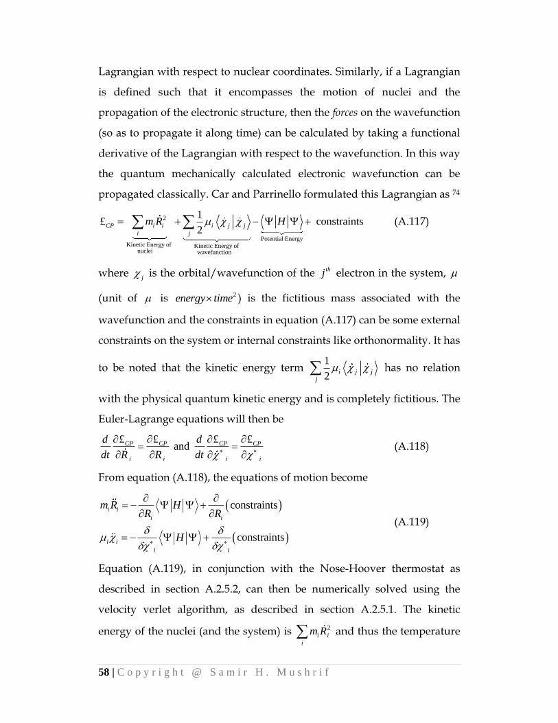
58 | C o p y r i g h t @ S a m i r H . M u s h r i f
Lagrangian with respect to nuclear coordinates. Similarly, if a Lagrangian
is defined such that it encompasses the motion of nuclei and the
propagation of the electronic structure, then the forces on the wavefunction
(so as to propagate it along time) can be calculated by taking a functional
derivative of the Lagrangian with respect to the wavefunction. In this way
the quantum mechanically calculated electronic wavefunction can be
propagated classically. Car and Parrinello formulated this Lagrangian as 74
2
Potential EnergyKinetic Energy of Kinetic Energy of nuclei wavefunction
1£ constraints
2CP i i i j j
i j
m R H (A.117)
where j is the orbital/wavefunction of the thj electron in the system,
(unit of is 2energy time ) is the fictitious mass associated with the
wavefunction and the constraints in equation (A.117) can be some external
constraints on the system or internal constraints like orthonormality. It has
to be noted that the kinetic energy term 1
2i j j
j
has no relation
with the physical quantum kinetic energy and is completely fictitious. The
Euler-Lagrange equations will then be
£ £ £ £ and CP CP CP CP
i i i i
d d
dt R R dt
(A.118)
From equation (A.118), the equations of motion become
constraints
constraints
i i
i i
i i
i i
m R HR R
H
(A.119)
Equation (A.119), in conjunction with the Nose-Hoover thermostat as
described in section A.2.5.2, can then be numerically solved using the
velocity verlet algorithm, as described in section A.2.5.1. The kinetic
energy of the nuclei (and the system) is 2
i i
i
m R and thus the temperature

59 | C o p y r i g h t @ S a m i r H . M u s h r i f
of the system 2
i i
i
T m R . Similarly the fictitious temperature associated
with the wavefunction is 1
2i j j
j
. A very small value of is
chosen so as to keep the fictitious temperature of the wavefunction very
low. The reason for this choice will become clear later. The main concerns
about the Car-Parrinello scheme would be as follows: (i) If the electronic
wavefunction follows the Born-Oppenheimer surface through out the
molecular dynamics simulation, (ii) How the forces calculated using Car-
Parrinello Lagrangian are equal to Born-Oppenheimer molecular
dynamics forces and (iii) How the total energy of the system is conserved
(microcanonical ensemble).15, 75
At the beginning of the Car-Parrinello molecular dynamics scheme,
the electronic wavefunction is optimized for the initial nuclear
configuration. When the nuclei start moving, their motion changes the
electronic structure of the system thereby changing the wavefunction
representing the minimum in the energy at an instantaneous nuclear
configuration. According to the Car-Parrinello Lagrangian, the
wavefunction is also propagated classically according to equation (A.119).
As mentioned before, the Car-Parrinello molecular dynamics will follow
the Born-Oppenheimer molecular dynamics when the wave function
propagated using the Car-Parrinello scheme will result in the same
electronic energy as that from the wavefunction which is optimized for the
modified Hamiltonian. This is only possible when no additional energy
from an external system (i.e. from the classical nuclear system) is
transferred to the classically propagated quantum electronic system;
because if the energy transfer occurs then the quantum system which is
propagated classically need to be treated quantum mechanically so as to
bring the electronic system to its minimum energy level. Also the “extra”
energy transferred to the wavefunction will result in larger forces on the

60 | C o p y r i g h t @ S a m i r H . M u s h r i f
wavefunction (in addition to i
H
), thereby deviating from the
Born-Oppenheimer surface. In other words, if the energy from the nuclei
is not transferred to the electronic system, the Car-Parrinello scheme
should follow the Born-Oppenheimer molecular dynamics. This
adiabaticity is achieved due to the virtue of the timescale difference
between the very fast electronic motion and the slow nuclear motion. It is
shown that when a small perturbation in the minimum energy state of a
system results in some force on the wavefunction, then the minimum
frequency related to the dynamics of the orbital is75
1
2
min
gapeE
(A.120)
where gapE is the energy difference between the highest occupied and the
lowest unoccupied orbital. The parameter gapE in equation (A.120) is
determined by the physics of the system, however, the parameter is
completely fictitious and hence can be fixed to an arbitrary value. The
frequency range of the orbital dynamics thus can be switched towards the
higher side by choosing a very small value of . If a sufficiently small
value is chosen then the power spectra emerging from the wavefunction
dynamics (fast motion, high frequency) can be completely separated from
that emerging from the nuclear dynamics (slow motion, low frequency). If
these two power spectra do not have any overlap in the frequency domain
then there will not be any energy transfer from the nuclei to the
wavefunction. Thus the fictitious kinetic energy of the wavefunction
1
2i j j
j
will remain constant. This fictitious kinetic energy is also a
measure of the correctness of the Car-Parrinello implementation. In this
way if the wavefunction or electronic structure during the Car-Parrinello

61 | C o p y r i g h t @ S a m i r H . M u s h r i f
molecular dynamics follows the Born-Oppenheimer surface then the
forces acting on the nuclei i
HR
will be the same as Born-
Oppenheimer molecular dynamics. The physical energy of the system is
2
i i
i
m R H , whereas the Car-Parrinello energy is
2 1
2i i i j j
i j
m R H . Since
21
2i j j i i
j i
m R H
(A.121)
and the fictitious kinetic energy remains constant, from statistical
mechanical point of view, it can be said that the system is under
microcanonical ensemble where the total energy of the system is
conserved. Figure A.6 shows various energies of a model system of bulk
crystalline silicon during the car-Parrinello run.
Figure A.6: Variation of different energies during the Car-Parrinello molecular dynamics run of bulk silicon. Adapted from Pastore and Smargiass75
A minute inspection of Fig. A.6 shows that the oscillations in the
fictitious kinetic energy are a mirror image of the oscillations in the
2 1
2i i i j j
i j
m R H
2
i i
i
m R H
H
1
2i j j
j

62 | C o p y r i g h t @ S a m i r H . M u s h r i f
potential energy of the system (a few order of magnitude difference
though). These can be attributed to the pull applied by the classically
moving nuclei on the classically propagating wavefunction.
A.2.7 Metadynamics
The Car-Parrinello molecular dynamics scheme, even though
significantly reduces the computational cost of ab initio molecular
dynamics, can not access the time scales more than a few picoseconds
when hundreds of atoms are present in the simulation system (even with
the state of the art computational servers). With the technological
evolution in computer hardware and reduction in costs, researchers are
hoping to increase the accessible length and timescales of ab-initio
molecular dynamics simulations. However, to run a simulation equivalent
to hundreds of nanoseconds (which is possible using classical force field
molecular dynamics) and to be able to simulate realistic phenomena
which take place at much larger timescales than that can be accessed by ab
initio molecular dynamics, in addition to the development of
computational hardware, it also becomes necessary to implement methods
that can accelerate the events somehow to make them happen earlier. Ab-
initio molecular dynamics is usually employed when chemical reactions
are taking place in the system and if the reaction of interest is associated
with a large energy barrier then the timescale for the reaction is large and
thus becomes difficult to be accessed using ab initio molecular dynamics.
Hence, a system may be stuck in a local minimum in the energy surface
and may take too long computational time to cross the energy barrier to
reach the global minimum (cf. Figure A.6).
The molecular dynamics simulation can be run at a higher
temperature so as to accelerate the event which is expected to take place at
a longer timescale in real system, however, this may cause some

63 | C o p y r i g h t @ S a m i r H . M u s h r i f
undesirable and unrealistic events to happen in the system. There are
several methods that have been implemented in the literature in the past
to overcome this difficulty including umbrella sampling,76 nudged elastic
band,77 finite temperature string method,78 transition path sampling,79
milestoning,80 multiple timescale accelerated molecular dynamics,81 to
name a few. The most recent of all these methods is called metadynamics82
and it has the following advantages:
1. It encompasses several benefits of all the above mentioned methods
2. It can accelerate the rare events so as to be able to see them in a
realistic computational simulation time.
3. It can also be used to reconstruct the energy surface so as to get
quantitative information about the energy landscapes and barriers.
4. It is coupled with the Car-Parrinello molecular dynamics by
Iannuzzi et al. very recently.83
The following two sub-sections describe the concept and mathematics
behind the metadynamics technique.

64 | C o p y r i g h t @ S a m i r H . M u s h r i f
Figure A.7: An illustration showing a large energy barrier for the system to go from a state A to the more stable state B.
A.2.7.1 Concept
The metadynamics technique, as described by Laio and Gervasio,82
is based on the principle of filling up the energy surface with potentials.
As shown in Figure A.8, if the energy surface is plotted as a one
dimensional function of a particular reaction coordinate and the system is
residing in the potential well ‘A’ from which it is taking too long to escape
due to the energy barriers then (cf. Figure A.7),
1. The potential well ‘A’ is filled up with small potentials so that
system slowly comes to a higher energy position.
2. As soon as the middle potential well is filled up, the system escapes
to the potential well ‘B’ on the left through the saddle point S1.
3. The potential well ‘B’ is then gradually filled till the saddle point S2
is reached then the system escapes to the potential well ‘C’.
4. Gradually, well ‘C’ is filled.
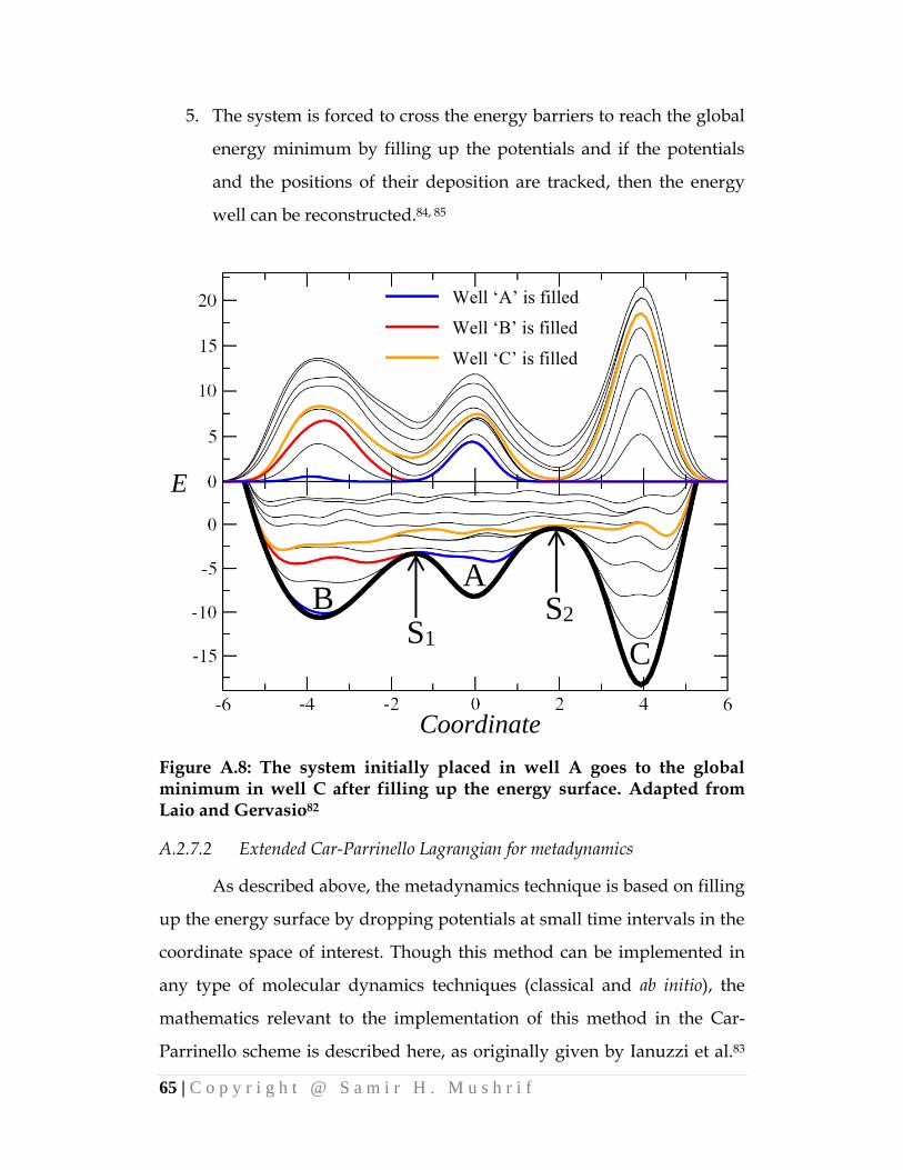
65 | C o p y r i g h t @ S a m i r H . M u s h r i f
5. The system is forced to cross the energy barriers to reach the global
energy minimum by filling up the potentials and if the potentials
and the positions of their deposition are tracked, then the energy
well can be reconstructed.84, 85
Figure A.8: The system initially placed in well A goes to the global minimum in well C after filling up the energy surface. Adapted from Laio and Gervasio82
A.2.7.2 Extended Car-Parrinello Lagrangian for metadynamics
As described above, the metadynamics technique is based on filling
up the energy surface by dropping potentials at small time intervals in the
coordinate space of interest. Though this method can be implemented in
any type of molecular dynamics techniques (classical and ab initio), the
mathematics relevant to the implementation of this method in the Car-
Parrinello scheme is described here, as originally given by Ianuzzi et al.83
A B
C S1
S2
E
Coordinate
—— Well ‘A’ is filled
—— Well ‘B’ is filled
—— Well ‘C’ is filled

66 | C o p y r i g h t @ S a m i r H . M u s h r i f
and further extended by Laio et al.82, 86-88 If ş is a vector of the collective
variables (coordinates of interest) that form the energy well to be filled or
that form the energy surface of interest (for ex. it can be the bond distance
between two hydrogen atoms if the dynamics and energy surface of
hydrogen dissociation is studied or it can be some coordination number if
a more complex phenomenon like protein conformation is studied), the
metadynamics approach treat them as additional variables in the system
and the car-Parrinello Lagrangian is then extended as 83
21
£ £ ş Ş ş ,2
MTD CP cv cv cv cv cv cv cv
cv cv
m k R t ş (A.122)
where £CP is the Lagrangian defined in equation A.117, the first term
indicates the kinetic energy of the collective variables, the second term is
the harmonic restraining potential and the last term is the potential that is
dropped to fill the energy well in the collective variable ş space at
different time intervals. Defining the kinetic and potential energy of the
additional collective variables allows controlling their dynamics in the
canonical ensemble using a suitable thermostat. The dynamics of ionic and
electronic (fictitious) motion are separated in the Car-Parrinello molecular
dynamics by choosing an appropriate value for the mass associated with
the fictitious kinetic energy of the wavefunction (as described in section
A.2.6.1). Analogous to the original Car-Parrinello scheme, the dynamics of
the collective variables are separated from the ionic and fictitious
electronic motion by choosing an appropriate value for the fictitious mass
cvm of the collective variables. If the fictitious mass cvm is large then the
dynamics of the collective variables will be slow and thus can be
separated from the ionic dynamics. The forces acting on the collective
variables are due to the potential energy Ş şcv cv cv cvk R
, and due to the
potential drops ,cv t ş . Hence the dynamics of the collective variables are

67 | C o p y r i g h t @ S a m i r H . M u s h r i f
also dependant on cvk . It has been shown that the extra term in
metadynamics introduces an additional frequency for the motion of
collective variables as cv cvk m 86. The force constant cvk is chosen such
that the collective variables are close to the actual coordinates of the
system. If a small cvk is used, it will result in a large variation in the
collective coordinate even with a small potential drop. However, a very
large value may result in very small timestep and excessive long
computational time. Since cvk is selected by the above constraints, it sets
limitation on the value of cvm so as to maintain the adiabaticity.
The potential used to fill the energy well at a time t is given as 82
22 1
2 4, exp exp
2 2i
i i ii
cv MTD
t ti
t Hw w
ş ş ş şş ş
ş (A.123)
where parameter MTDH is the height of the Gaussian. The first term in the
above functional form of the potential is a typical Gaussian which is then
multiplied with another Gaussian of width 1i i
iw ş ş . This
mathematical manipulation narrows the width of the potential in the
direction of the trajectory, thus depositing the potentials close to each
other in the direction of the trajectory. The values of the height and width
of Gaussian depends upon the topology of the energy landscape of the
system under investigation.86
Metadynamics using an extended Car-Parrinello Lagrangian has
recently been implemented to study glycine and pyrite surface
interactions,89 isomerisation of alanine dipeptide,90 azulene to naphthalene
rearrangement,91 proton diffusion in molecular crystals,92 to name a few.

68 | C o p y r i g h t @ S a m i r H . M u s h r i f
A.3 References
1. Poirier, E.; Chahine, R.; Bose, T. K., Hydrogen adsorption in carbon
nanostructures. International Journal of Hydrogen Energy 2001, 26, (8), 831-
835.
2. Basova, Y. V.; Edie, D. D., Precursor chemistry effects on particle
size and distribution in metal-containing pitch-based carbon fibers - an
hypothesis. Carbon 2004, 42, (12-13), 2748-2751.
3. Jang, J. W.; Lee, C. E.; Oh, C. I.; Lee, C. J., Hydrogen storage
capacity of different carbon nanostructures in ambient conditions. Journal
of Applied Physics 2005, 98, (7), 074316-1-3.
4. Gallego, N. C.; Contescu, C. I.; Bhat, V. V.; Benthem, K. V.;
Tekinalp, H.; Edie, D. D., Palladium-doped nanoporous carbon fibers for
hydrogen storage In International conference on Carbon, Nagano, Japan,
2008.
5. Lachawiec, A. J.; Qi, G. S.; Yang, R. T., Hydrogen storage in
nanostructured carbons by spillover: Bridge-building enhancement.
Langmuir 2005, 21, (24), 11418-11424.
6. Li, Y. W.; Yang, F. H.; Yang, R. T., Kinetics and mechanistic model
for hydrogen spillover on bridged metal-organic frameworks. Journal of
Physical Chemistry C 2007, 111, (8), 3405-3411.
7. Jensen, F., Introduction to Computational Chemistry. John Wiley &
Sons Ltd.: West Sussex, 2007.
8. Peslherbe, G. H., Lecture Notes. In Concordia University: Montreal,
2006.
9. Comba, P.; Kerscher, M., Computation of structures and properties
of transition metal compounds. Coordination Chemistry Reviews 2009, 253,
(5-6), 564-574.

69 | C o p y r i g h t @ S a m i r H . M u s h r i f
10. Deeth, R. J., The ligand field molecular mechanics model and the
stereoelectronic effects of d and s electrons. Coordination Chemistry Reviews
2001, 212, 11-34.
11. Deeth, R. J.; Anastasi, A.; Diedrich, C.; Randell, K., Molecular
modelling for transition metal complexes: Dealing with d-electron effects.
Coordination Chemistry Reviews 2009, 253, (5-6), 795-816.
12. Jensen, F.; Norrby, P. O., Transition states from empirical force
fields. Theoretical Chemistry Accounts 2003, 109, (1), 1-7.
13. Marx, D.; Hutter, J., Ab-initio molecular dynamics: Theory and
implementation. In Modern Methods and Algorithms of Quantum Chemistry
Proceedings, Grotendorst, J., Ed. John von Neumann Institute for
Computing: Forschungszentrum Jülich, 2000; Vol. 1, pp 301-449.
14. Norrby, P. O.; Brandt, P., Deriving force field parameters for
coordination complexes. Coordination Chemistry Reviews 2001, 212, 79-109.
15. Payne, M. C.; Teter, M. P.; Allan, D. C.; Arias, T. A.; Joannopoulos,
J. D., Iterative Minimization Techniques for Abinitio Total-Energy
Calculations - Molecular-Dynamics and Conjugate Gradients. Reviews of
Modern Physics 1992, 64, (4), 1045-1097.
16. Remler, D. K.; Madden, P. A., Molecular-Dynamics without
Effective Potentials Via the Car-Parrinello Approach. Molecular Physics
1990, 70, (6), 921-966.
17. All the papers in Coordination Chemistry Reviews, vol. 212, Issue 1
In pp 1-168.
18. Duin, A. v. ReaxFF user manual; California Institute of Technology:
Pasadena, 2002; pp 1-39.
19. Comba, P., The Relation between Ligand Structures, Coordination
Stereochemistry, and Electronic and Thermodynamic Properties.
Coordination Chemistry Reviews 1993, 123, (1-2), 1-48.
70 | C o p y r i g h t @ S a m i r H . M u s h r i f
20. Comba, P., Solution Structures of Coordination Compounds.
Comments on Inorganic Chemistry 1994, 16, 133-151.
21. Comba, P., Strains and stresses in coordination compounds.
Coordination Chemistry Reviews 1999, 182, 343-371.
22. Comba, P.; Hambley, T. W., Molecular Modeling of Inorganic
Compounds. VCH: New York, 1995.
23. Comba, P.; Zimmer, M., Inorganic molecular mechanics. Journal of
Chemical Education 1996, 73, (2), 108-110.
24. Cundari, T. R., Molecular modeling of d- and f-block metal
complexes. Journal of the Chemical Society-Dalton Transactions 1998, (17),
2771-2776.
25. Hay, B. P., Methods for Molecular Mechanics Modeling of
Coordination-Compounds. Coordination Chemistry Reviews 1993, 126, (1-2),
177-236.
26. Landis, C. R.; Root, D. M.; Cleveland, T., Molecular Mechanics
Force Fields for Modeling Inorganic and Organometallic Compounds. In
Reviews in Computational Chemistry, Lipkowitz, K. B.; Boyd, D. B., Eds.
Wiley-VCH: Toronto, 2007; Vol. 6, pp 73-148.
27. Zimmer, M., Bioinorganic molecular mechanics. Chemical Reviews
1995, 95, (8), 2629-2649.
28. Gajewski, J. J.; Gilbert, K. E.; Kreek, T. W., General molecular
mechanics approach to transition metal complexes. Journal of
Computational Chemistry 1998, 19, (10), 1167-1178.
29. Rappe, A. K.; Casewit, C. J.; Colwell, K. S.; Goddard, W. A.; Skiff,
W. M., Uff, a Full Periodic-Table Force-Field for Molecular Mechanics and
Molecular-Dynamics Simulations. Journal of the American Chemical Society
1992, 114, (25), 10024-10035.
30. Rappe, A. K.; Casewit, C. J., Molecular Mechanics Across Chemistry.
University Science Books: Sausalito, California, 1997.

71 | C o p y r i g h t @ S a m i r H . M u s h r i f
31. Comba, P.; Hambley, T. W.; Okon, N.; Lauer, G. MOMEC97 A
Molecular Modeling Package for Inorganic Compounds, Heidelberg, 1997.
32. Bernhardt, P. V.; Comba, P., Molecular Mechanics Calculations of
Transition-Metal Complexes. Inorganic Chemistry 1992, 31, (12), 2638-2644.
33. Boeyens, J. C. A.; Comba, P., Molecular mechanics: theoretical basis,
rules, scope and limits. Coordination Chemistry Reviews 2001, 212, 3-10.
34. Nava, P.; Sierka, M.; Ahlrichs, R., Density functional study of
palladium clusters. Physical Chemistry Chemical Physics 2003, 5, (16), 3372-
3381.
35. Schrodinger, E., An undulatory theory of the mechanics of atoms
and molecules. Physical Review 1926, 28, (6), 1049-1070.
36. Bredow, T.; Jug, K., Theory and range of modern semiempirical
molecular orbital methods. Theoretical Chemistry Accounts 2005, 113, (1), 1-
14.
37. Sherrill, C. D.; Schaefer, H. F., The configuration interaction
method: Advances in highly correlated approaches. Advances in Quantum
Chemistry, Vol 34 1999, 34, 143-269.
38. Bartlett, R. J., Coupled-Cluster Approach to Molecular-Structure
and Spectra - a Step toward Predictive Quantum-Chemistry. Journal of
Physical Chemistry 1989, 93, (5), 1697-1708.
39. Moller, C.; Plesset, M. S., Note on an approximation treatment for
many-electron systems. Physical Review 1934, 46, (7), 0618-0622.
40. Hohenberg, P.; Kohn, W., Inhomogeneous Electron Gas. Physical
Review B 1964, 136, (3B), B864-B871.
41. Thomas, L. H., The calculation of atomic fields. Proceedings of the
Cambridge Philosophical Society 1927, 23, 542-548.
42. Fermi, E., Un Metodo Statistico per la Determinazione di alcune
Priorieta dell'Atome. Rend. Accad. Naz. Lincei. 1927, 6, 602-607.

72 | C o p y r i g h t @ S a m i r H . M u s h r i f
43. Kohn, W.; Sham, L. J., Self-Consistent Equations Including
Exchange and Correlation Effects. Physical Review 1965, 140, (4A), 1133-
1138.
44. Parr, R. G.; Yang, W., Density-Functional Theory of Atoms and
Molecules. Oxford University Press: Oxford, 1989.
45. Dirac, P. A. M., Note on exchange phenomena in the Thomas atom.
Proceedings of the Cambridge Philosophical Society 1930, 26, 376-385.
46. Ceperley, D. M.; Alder, B. J., Ground-State of the Electron-Gas by a
Stochastic Method. Physical Review Letters 1980, 45, (7), 566-569.
47. Vosko, S. H.; Wilk, L.; Nusair, M., Accurate Spin-Dependent
Electron Liquid Correlation Energies for Local Spin-Density Calculations -
a Critical Analysis. Canadian Journal of Physics 1980, 58, (8), 1200-1211.
48. Becke, A. D., Density-Functional Thermochemistry .2. The Effect of
the Perdew-Wang Generalized-Gradient Correlation Correction. Journal of
Chemical Physics 1992, 97, (12), 9173-9177.
49. Becke, A. D., Density-Functional Thermochemistry .1. The Effect of
the Exchange-Only Gradient Correction. Journal of Chemical Physics 1992,
96, (3), 2155-2160.
50. Becke, A. D., Density-Functional Thermochemistry .3. The Role of
Exact Exchange. Journal of Chemical Physics 1993, 98, (7), 5648-5652.
51. Lee, C. T.; Yang, W. T.; Parr, R. G., Development of the Colle-
Salvetti Correlation-Energy Formula into a Functional of the Electron-
Density. Physical Review B 1988, 37, (2), 785-789.
52. Perdew, J. P.; Burke, K.; Ernzerhof, M., Generalized gradient
approximation made simple. Physical Review Letters 1996, 77, (18), 3865-
3868.
53. Perdew, J. P.; Chevary, J. A.; Vosko, S. H.; Jackson, K. A.; Pederson,
M. R.; Singh, D. J.; Fiolhais, C., Atoms, Molecules, Solids, and Surfaces -
73 | C o p y r i g h t @ S a m i r H . M u s h r i f
Applications of the Generalized Gradient Approximation for Exchange
and Correlation. Physical Review B 1992, 46, (11), 6671-6687.
54. Perdew, J. P.; Yue, W., Accurate and Simple Density Functional for
the Electronic Exchange Energy - Generalized Gradient Approximation.
Physical Review B 1986, 33, (12), 8800-8802.
55. Meyer, B., The pseudopotential planewave approach. In
Computational Nanoscience: Do It Yourself!, Grotendorst, J.; Blügel, S.; Marx,
D., Eds. John von Neumann Institute for Computing: Forschungszentrum
Jülich, 2006; Vol. 31, pp 1-13.
56. Kittel, C., Introduction to Solid State Physics. Wiley: New York, 1996.
57. Evarestov, R. A.; Smirnov, V. P., Special Points of the Brillouin-
Zone and Their Use in the Solid-State Theory. Physica Status Solidi B-Basic
Research 1983, 119, (1), 9-40.
58. Hamann, D. R.; Schluter, M.; Chiang, C., Norm-Conserving
Pseudopotentials. Physical Review Letters 1979, 43, (20), 1494-1497.
59. Kerker, G. P., Non-Singular Atomic Pseudopotentials for Solid-
State Applications. Journal of Physics C-Solid State Physics 1980, 13, (9),
L189-L194.
60. Troullier, N.; Martins, J. L., Efficient Pseudopotentials for Plane-
Wave Calculations. Physical Review B 1991, 43, (3), 1993-2006.
61. Hutter, J. Lecture Notes: Introduction to ab-initio molecular dynamics;
Zurich, 2002; pp 1-119.
62. Stich, I.; Car, R.; Parrinello, M., Structural, Bonding, Dynamic, and
Electronic-Properties of Liquid Silicon - an Abinitio Molecular-Dynamics
Study. Physical Review B 1991, 44, (9), 4262-4274.
63. Kleinman, L.; Bylander, D. M., Efficacious Form for Model
Pseudopotentials. Physical Review Letters 1982, 48, (20), 1425-1428.
64. Raugei, S. Implementation of DFT based Car-Parrinello molecular
dynamics; Trieste, Italy, 2007; pp 1-23.

74 | C o p y r i g h t @ S a m i r H . M u s h r i f
65. Goedecker, S.; Teter, M.; Hutter, J., Separable dual-space Gaussian
pseudopotentials. Physical Review B 1996, 54, (3), 1703-1710.
66. Hartwigsen, C.; Goedecker, S.; Hutter, J., Relativistic separable
dual-space Gaussian pseudopotentials from H to Rn. Physical Review B
1998, 58, (7), 3641-3662.
67. Verlet, L., Computer Experiments on Classical Fluids .I.
Thermodynamical Properties of Lennard-Jones Molecules. Physical Review
1967, 159, (1), 98-103.
68. Andersen, H. C., Molecular-Dynamics Simulations at Constant
Pressure and-or Temperature. Journal of Chemical Physics 1980, 72, (4),
2384-2393.
69. Hoover, W. G., Canonical Dynamics - Equilibrium Phase-Space
Distributions. Physical Review A 1985, 31, (3), 1695-1697.
70. Nose, S., A Molecular-Dynamics Method for Simulations in the
Canonical Ensemble. Molecular Physics 1984, 52, (2), 255-268.
71. Hunenberger, P., Thermostat algorithms for molecular dynamics
simulations. Advanced Computer Simulation Approaches for Soft Matter
Sciences I 2005, 173, 105-147.
72. Martyna, G. J.; Klein, M. L.; Tuckerman, M., Nose-Hoover Chains -
the Canonical Ensemble Via Continuous Dynamics. Journal of Chemical
Physics 1992, 97, (4), 2635-2643.
73. Toxvaerd, S.; Olsen, O. H., Canonical Molecular-Dynamics of
Molecules with Internal Degrees of Freedom. Berichte Der Bunsen-
Gesellschaft-Physical Chemistry Chemical Physics 1990, 94, (3), 274-278.
74. Car, R.; Parrinello, M., Unified Approach for Molecular-Dynamics
and Density-Functional Theory. Physical Review Letters 1985, 55, (22), 2471-
2474.
75. Pastore, G.; Smargiassi, E.; Buda, F., Theory of Abinitio Molecular-
Dynamics Calculations. Physical Review A 1991, 44, (10), 6334-6347.

75 | C o p y r i g h t @ S a m i r H . M u s h r i f
76. Torrie, G. M.; Valleau, J. P., Non-Physical Sampling Distributions in
Monte-Carlo Free-Energy Estimation - Umbrella Sampling. Journal of
Computational Physics 1977, 23, (2), 187-199.
77. Henkelman, G.; Jonsson, H., Improved tangent estimate in the
nudged elastic band method for finding minimum energy paths and
saddle points. Journal of Chemical Physics 2000, 113, (22), 9978-9985.
78. Weinan, E.; Ren, W. Q.; Vanden-Eijnden, E., Finite temperature
string method for the study of rare events. Journal of Physical Chemistry B
2005, 109, (14), 6688-6693.
79. Dellago, C.; Bolhuis, P. G.; Csajka, F. S.; Chandler, D., Transition
path sampling and the calculation of rate constants. Journal of Chemical
Physics 1998, 108, (5), 1964-1977.
80. Faradjian, A. K.; Elber, R., Computing time scales from reaction
coordinates by milestoning. Journal of Chemical Physics 2004, 120, (23),
10880-10889.
81. Miron, R. A.; Fichthorn, K. A., Multiple-time scale accelerated
molecular dynamics: Addressing the small-barrier problem. Physical
Review Letters 2004, 93, (12), 128301-1-12.
82. Laio, A.; Gervasio, F. L., Metadynamics: a method to simulate rare
events and reconstruct the free energy in biophysics, chemistry and
material science. Reports on Progress in Physics 2008, 71, (12), 126601-1-22.
83. Iannuzzi, M.; Laio, A.; Parrinello, M., Efficient exploration of
reactive potential energy surfaces using Car-Parrinello molecular
dynamics. Physical Review Letters 2003, 90, (23), 228302-1-4.
84. Bussi, G.; Laio, A.; Parrinello, M., Equilibrium free energies from
nonequilibrium metadynamics. Physical Review Letters 2006, 96, (9),
090601-1-4.

76 | C o p y r i g h t @ S a m i r H . M u s h r i f
85. Laio, A.; Rodriguez-Fortea, A.; Gervasio, F. L.; Ceccarelli, M.;
Parrinello, M., Assessing the accuracy of metadynamics. Journal of Physical
Chemistry B 2005, 109, (14), 6714-6721.
86. Ensing, B.; Laio, A.; Parrinello, M.; Klein, M. L., A recipe for the
computation of the free energy barrier and the lowest free energy path of
concerted reactions. Journal of Physical Chemistry B 2005, 109, (14), 6676-
6687.
87. Laio, A.; Parrinello, M., Escaping free-energy minima. Proceedings of
the National Academy of Sciences of the United States of America 2002, 99, (20),
12562-12566.
88. Laio, A.; Parrinello, M., Computing Free Energies and Accelerating
Rare Events with Metadynamics. In Computer Simulations in Condensed
Matter Systems: From Materials to Chemical Biology, Springer Berlin:
Heidelberg, 2006; Vol. 1, pp 315-347.
89. Nair, N. N.; Schreiner, E.; Marx, D., Glycine at the Pyrite–Water
Interface: An ab initio Metadynamics Study. In NIC Symposium 2008,
Munster, G.; Wolf, D.; Kremer, M., Eds. John von Neumann Institute for
Computing: Julich, 2008; Vol. 39, pp 101-108.
90. Branduardi, D.; Gervasio, F. L.; Parrinello, M., From A to B in free
energy space. Journal of Chemical Physics 2007, 126, (5), 054103-1-10.
91. Stirling, A.; Iannuzzi, M.; Laio, A.; Parrinello, M., Azulene-to-
naphthalene rearrangement: The Car-Parrinello metadynamics method
explores various mechanisms. Chemphyschem 2004, 5, (10), 1558-1568.
92. Iannuzzi, M.; Parrinello, M., Proton transfer in heterocycle crystals.
Physical Review Letters 2004, 93, (2), 025901-1-4.