A MODIFIED SEPARABLE PROGRAMMINGAPPROACH TO WEAPON SYSTEM

ALLOCATION PROBLEMS

Thomas Robert McLaughlin

Library

Naval Postgraduate School

Monterey, California 93940

h SO

Monterey, California

THESIA MODIFIED SEPARABLE PROGRAMMING

APPROACH TO WEAPON SYSTEM ALLOCATION PROBLEMS

by

Thomas Robert McLaughlin Jr

Thesis Advisor James G. Taylor

March 1973

Approved £oi puhtlc fi<Ltzai><i; dc6 tnlhuXioYi antimitud

.

T153556

A Modified Separable ProgrammingApproach to Weapon System Allocation Problems

by

Thomas Robert McLaughlin JrCaptain, United States Army

B.S., United States Military Academy, 1966

Submitted in partial fulfillment of therequirements for the degree of

MASTER OF SCIENCE IN OPERATIONS RESEARCH

from the

NAVAL POSTGRADUATE SCHOOLMarch 1973

Library

Naval Postgraduate SchoolMonterey, Califor

ABSTRACT

This thesis considers mathematical techniques for com-

puting the optimal allocation of weapons from m different

systems against n undefended targets. A standard nonlinear

programming problem is considered. A discussion is given

on John Danskin's Algorithm for the determination of the

optimal values of the lagrange multipliers for this problem

Using a transformation of variables, the nonlinear problem

is reformulated as a separable problem and solved by sepa-

rable programming. A new method, the hybrid algorithm, for

the determination of the optimal lagrange multipliers is

developed.

TABLE OF CONTENTS

I. INTRODUCTION - 4

II. MATHEMATICAL MODELS FOR THE ALLOCATIONOF WEAPONS TO TARGETS --- 5

A. AERIAL BOMBING MODEL - 6

B. "BLACK AND WHITE" TARGET MODEL 8

C. NUCLEAR WARHEAD MODEL -- 9

III. THE DETERMINATION OF NECESSARY ANDSUFFICIENT CONDITIONS 12

IV. NUMERICAL METHODS OF SOLUTION - 16

A. DANSKIN'S ALGORITHM 16

B. SEPARABLE PROGRAMMING 18

C. HYBRID ALGORITHM --- 2 5

V. EXTENSION OF MODEL AND SOLUTION - 30

APPENDIX A Heuristic Presentation of Danskin'sMethod with Slight Modification - 32

APPENDIX B Worked Numerical Examples of theSeparable Programming Method 44

APPENDIX C Worked Numerical Examples of theHybrid Method -- - 46

COMPUTER PROGRAM - - -- 51

LIST OF REFERENCES - 59

INITIAL DISTRIBUTION LIST 61

FORM DD 1473 -- - - --- 63

I. INTRODUCTION

As a result of today's production costs, armament trea-

ties, and stockpiling facilities, both military tacticians

and civilian defense planners are constantly confronted

with the decision of how to optimally allocate offensive

weapons such as ICBMs, SLBMs, bombs and artillery rounds to

various military/industrial targets. Models with varying

degrees of complexity and measures of effectiveness have

been devised to assist in this decision.

This thesis concerns itself with solving these offensive

weapon systems assignment problems so as to optimize measure-

able returns such as damage or monetary savings. A non-

linear model for an offensive allocation to a group of

undefended targets is presented. An algorithm devised by

John Danskin [Ref. 1] for obtaining the optimal lagrange

multipliers and hence the constrained optima to this problem

is discussed and illustrated with an example. The model is

then transformed to a separable problem and an approximate

solution is obtained utilizing separable programming.

Using separable programming and the Kuhn-Tucker conditions,

the thesis then proceeds to develop and apply a new method

called the hybrid algorithm for calculating the optimal

lagrange multipliers and then the optimal allocations.

I I . MATHEMATICAL MODELS FOR THE ALLOCATIONOF WEAPONS TO TARGETS

The models considered in this paper are those that have

a nonlinear objective function and linear constraints. The

three specific models presented are those dealing with aerial

bombing, "black and white" targets, and nuclear weapons.

These three models have two similarities in common. First,

the nonlinear function is directly dependent on the military/

industrial target value, the number of weapons allocated,

and the weapon's effectiveness/ineffectiveness against a

target. Secondly, the linear constraint restricts the

number of weapons allocated so as not to exceed the total

number stockpiled or available.

Similar weapon allocation models, considering some form

of cost, have been developed. Examples of these are the

allocation of weapons so as to inflict maximum damage with

minimum delivery cost, or optimization of production costs

subject to a budgetary constraint. This class of models

will not be considered in this thesis, but any method

presented may be modified to handle such cases.

The basic assumptions relevant to all the following

weapon allocation models are:

1. The attack time is of short duration so as to

preclude an effectiveness evaluation of preceding

rounds

.

2. Target location is fixed.

3. Multiple kill by a single round is prohibited.

4. The effectiveness of each individual weapon is

independent

.

A. AERIAL BOMBING MODEL

This model was developed by Kooprnan in Ref. 1. It is a

model that might be used to allocate weapons, of differing

magnitude, delivered by aerial bombardment. The total dam-

age inflicted by the bombardment is related to the number

of direct hits by a lethality function. This function re-

duces the target value by some fractional amount of its

previous value. A lethality function representing y direct

hits might be written as

V(y) = V-ky where O^k^l (1)

or in terms of damage as

D(y) = V.d-k^). (2)

If more than one type of weapon is used, the damage function

takes on the form

D(y) = V.(1-.TT k. 7i ). (3)J

1_i 1

Kooprnan assumes that each individual weapon (bomb) acts

independently and that each bomb of type i has a probabil-

ity P.. of hitting target j. Thus, the probability that y

hits occur out of the x. bombs dropped on target j is

P(y) = i^Cypp/iU-Pi) ^ yi(4)

and the expected damage takes the form

(

ty'lwtWm

9^f"" (5)

An application o£ Newton's binomial theorem reduces the

expected damage formula to

f\

dW\ m/-TT

_ ''J 1J\_

>

< J

(6)

Thus, the basic model to be used to allocate the aerial

weapons is one that maximizes the expected damage subject

to the number of bombs available and is stated as

\

nmaximize ]£, V\

J-' J

no/-IT *l s

\

subject to: z.%. — A where i = l,2,...,mU '

(7)

and

is an interger.

In order to transform this model into a more mathematically

tractable form the following approximation is utilized.

Lemma If N is a large integer and

then

p(l-k) is small,

/- /-JDU-A

i/V -uM

-/-e-M

where rp •-k\

Proof

/-

/-

/-f>y-k\

/-p\/-A

H * i m \k= /-zW-/

to\k\ IPh-k

M

k

rN

/- /-/Vpl /-AYand also

4-H ^ p\J-km ~P A/

thus-juA/

/-e' -/ /--/>M /V

J

Hence, the basic aerial bombing model is now restated as

maxim" I m /

ize Z V.< /-rr e^p -jw #

subject to: Z, % — Xj=l

!i

(8)

/

where i 1 , 2 , . . . ,m

x ^ o.

B. "BLACK AND WHITE" TARGET MODEL

This model was discussed by Danskin in Ref. 2 and is

similar to those published by denBroeder, Ellison, and

Emerling [Ref. 3] and Mylander [Ref. 4] . A "black and

white" target is one that is either destroyed or not affected

by the incoming weapon system, such as missile silos, or

other undefended small point targets. Considering the case

of m different weapon systems and n "black and white"

targets, the kill probability of one weapon from each of

these independent weapon systems is

8

1-(1-P1)...(1-P

B) (9)

By letting,

/-/> = c M ...,/-P = e~Mr"

(10)

expression (9) is expressed as

en)

I£ there were x. weapons allocated, expression (11) is re

written as

/- e-/W-" •-/*m*n

(12)

and the basic model for all the "black and white" targets

would be stated as

maximize Z. V.

m/-eip- £^rs/VoU

(13)

subject to: ^ nJ -J,

where i 1 , 2 , . . . ,m

x. ; ^ 0.

C. NUCLEAR WARHEAD MODEL

This model was first discussed and published by Lemus

and David [Ref . 5] . It deals with the problem of allocat-

ing nuclear weapons of varying yields to relatively defense

less targets. Associated with each weapon system is a

launch reliability, R.., a nuclear yield, y., a circular

error probable, CEP., and a probability of penetrating

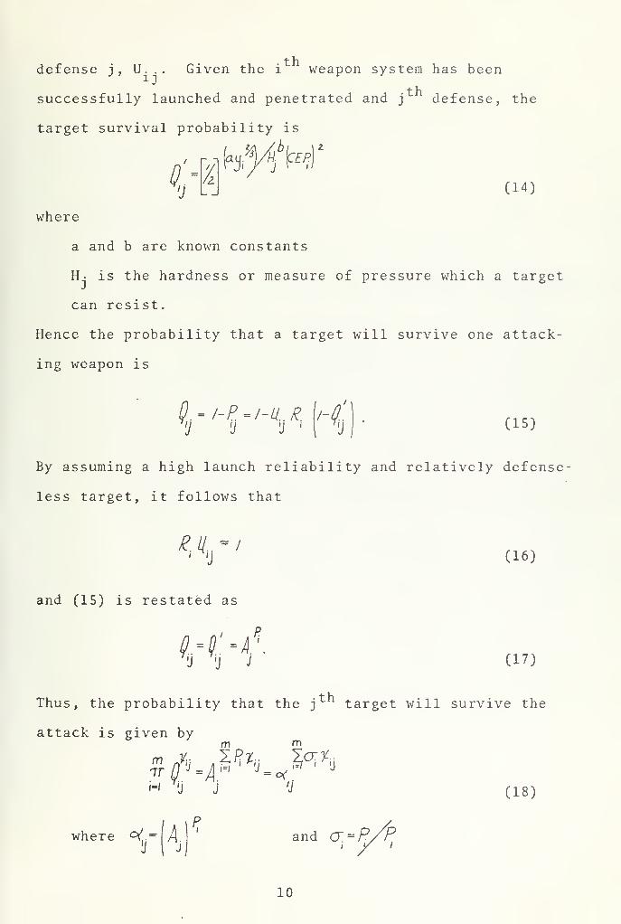
+ Vi

defense j, U. .. Given the i weapon system has been+ v>

successfully launched and penetrated and j defense, the

target survival probability is

i- /z

b^jW(14)

where

a and b are known constants

H- is the hardness or measure of pressure which a target

can resist.

Hence the probability that a target will survive one attack-

ing weapon is

0. -/-£-/-£.£ (/_/?'

'J 'J U ' U(15)

By assuming a high launch reliability and relatively defense

less target, it follows that

'

'J(16)

and (15) is restated as

•j u j (17)

Thus, the probability that the j target will survive the

attack is given bym nn

H Tj

j j 'J (18)

where o(=\J\!/ 1 J

and a-R/P

10

Hence, the basic nuclear weapon model, maximizing the value

of the targets destroyed, subject to the restriction that

the total weapons allocated does not exceed the number

available, is expressed as

m

maximizen

j- J J

S^iVi/-°<

1=/ I I

'J

(19)

subject to: X £ — X where i = l,2,...,m

x. .^0

11

III. THE DETERMINATION OF NECESSARYAND SUFFICIENT CONDITIONS

All subsequent work and calculations, deal only with

models of the aerial bombing or "black and white" target

form. If the reader desires to use the nuclear warhead mod-

el, all formulas and programs must be changed to account

for the new constant o( . . .

The necessary and sufficient conditions for the optimal

solution to the weapon system allocation model, are obtained

by a direct application of the Kuhn-Tucker theorem. The

reader can find a complete discussion of the Kuhn-Tucker

conditions in Ref s . 6 and 7. For the model,

n

maximize X V

subject to: X % — X. where i= 1 , 2 , , . ..,m

J=l

'J

x. .> 0,

the Kuhn-Tucker theorem yields the following conditions

x*x* = 0<=W M e"^ J- X* - or (20)3 3 j

:.>0^=^V.^.e'^j xj= A <JU.V.,

3 3r3 'j 3

(21)

12

thus

,

*:. = 1/M. 1

3 ' J

/ JU-V-n 'vi

The following lemma shows, by contradiction, that the

lagrange multiplier must be greater than zero and hence the

constraint is active.

Lemma The lagrange multiplier, (X* )>0.

Proof Assume \*=0.

then X*=0 <}

JjVj>Vy

x. >0.J

thus

But the Kuhn-Tucker conditions require that

* —

/

%. =ft In + CO = +oo > XX.

Hence, \* must be greater than zero. The Kuhn-

Tucker complementary slackness conditions require

that

X 1% -x -0

Since \* > , then .Z, x = X. QEDJ= 1

J

Extending the above to the model consisting of m weapon

systems and n targets, the Kuhn-Tucker necessary and suffi

cient conditions become

ij r'j J r

m

L k*Vy<

X*(22)

'Jn

j JI

m-IZ. U % x* (23)

13

For any given target j, there are three possible cases that

can occur during the allocation process. Either the target

will have no weapon system allocated to it, one weapon

system allocated, or more than one weapon system allocated.

In the first case, for a given target j, all x. .=0 and the

Kuhn-Tucker conditions reduce to the form

i

11. =0<=>u V ^X for all i = l,2,...,m (24)

The second case requires that x, .=0 for all weapon systems

k=l , 2 , . . . , i- 1 , i+1 , . . . ,m and x,.>0. For this allocation,il

the Kuhn-Tucker conditions become

X

K/j«PL i

u t

= x:

i L r M iij'J 'J

X*

(25)

andv.

<

Vje*/WjJ~\

r *i -x:

e^P -u.X.'Lr,

J li

J

Hence

(26)

(27)

and x^inK.V,

X"

(28)

The final case is just an extension of the preceding one.

For this case, the Kuhn-Tucker conditions become

14

u..v. exp$>»^ ^u

=X* for all i where x. > (29)1 J

and p V. exp

Hence

13 J

X*

'A for all k where x. .=0.k

k J

H'J

= a constant for all x..>0.

(30)

(31)

Which implies that

£< &hj H

^J

and 2 u. « =//)£>0 r'J 'J

rj J

X*

for all x*.>0, x* =0 (32)ij kj

for all i where x >0. (33)

15

IV. NUMERICAL METHODS OF SOLUTION

With the development of high speed computers many-

analytical and iterative methods have been devised for

yielding exact and approximate solutions to the problem.

Almost all methods treat the weapons as a continuous vari-

able. Consequently an "eye ball" rounding approximation

must be made for the final allocation. This thesis con-

siders the Danskin solution, which is an exact solution,

the separable programming approximation, and the hybrid

exact solution method.

Other methods available, but not examined include

Sequential Unconstrained Minimization Technique (SUMT) by

Mylander [Ref. 4], geometeric programming by Passy [Ref.8],

treatment as a transportation problem by Manne [Ref. 9] , and

other analytical algorithms by denBroeder, Ellison, and

Emerling [Ref. 3] , and Lemus and David [Ref. 5]

.

A. DANSKIN' S ALGORITHM

One of the earliest algorithms for an exact solution

was devised by John Danskin [Ref. 2] in the early 1950's.

Danskin' s algorithm uses the previously discussed Kuhn-

Tucker necessary and sufficient conditions, Gibbs Lemma,

and the concept of marginal return, to obtain the optimal

lagrange multiplier.

Gibbs Lemma is discussed in Ref. 2

16

The algorithm as applied to the one weapon system n

target model consists of the following steps.

Step 1 Consider the quantity M- V and arrange theJ J

target listing so that Aa.V. ^ u. . V forr) J /j + 1 j + 1

Step 2

Step 3

all j.

Define the function

5/

XI- Z% XI- Z„ A InI j-i'jl ly* J

u.V.

iir (34)

where A denotes a trial value for the optimal

value of the lagrange multiplier A, and x ( X )

j

is a trial allocation. Next find the largest

(35)

index such that

s( X = /^.v.) ^ x.

Denote this index as j=L.

Once L is known (and hence the targets in the

"optimal target list") , A may be explicitly

determined. From the Kuhn-Tucker conditions

5 X--X-I TT/a7

J" ^

step 2

/a

h V.

J J

X*

and from (36)

S X-tiVl-2 TT In\ nu N rj

t*1/

u.U V (37)

both of which contain the same list of regions

Subtracting (37) from (36) we obtain a formula

for the optimal lagrange multiplier,

17

^'h^L^P(38)

Knowing the index L, A may also be calculated

by the formula

X - epp <

j=i W-*^ / >- (39)

;

Step 4 Once A has been found, the Kuhn-Tucker nec-

essary and sufficient conditions can be

utilized to obtain the optimal allocation.

The algorithm as applied to more than one weapon system

is much more complex and requires a computer program to

obtain the optimal target listing. A discussion of a

typical computer program may be found in Ref. 10. Appendix

A, of this thesis gives a heuristic approach to Danskin's

algorithm for one and two weapon system model.

B. SEPARABLE PROGRAMMING

Separable programming is used to obtain an approximate

solution to nonlinear functions having a separable objec-

tive function and constraint. A separable function is any

general function that can be written in the form f (x ,x , .

.

x„)= y f.(x.)> where f.(x.) is a function of the singlen jiq ii 11

variable x.. A separable problem takes the form

18

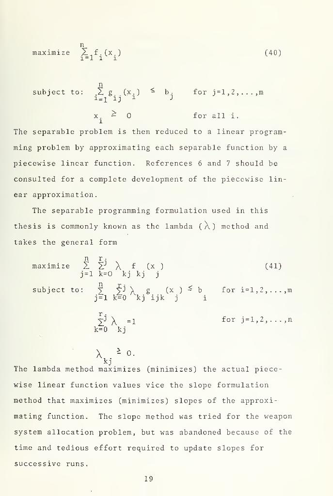
nmaximize Z £. (x ) (40)

1 = 1 1 l

nsubject to: X g (x.) - b- for j=l,2,...,m

i=l ij 1 3

x. - for all i.l

The separable problem is then reduced to a linear program-

ming problem by approximating each separable function by a

piecewise linear function. References 6 and 7 should be

consulted for a complete development of the piecewise lin-

ear approximation.

The separable programming formulation used in this

thesis is commonly known as the lambda (X) method and

takes the general form

n r -

maximize X X A f (x ) (41)j=l k=0 kj kj j

n r •

subject to: £ X"1 X 2 (x ) b for i=l,2,...,m

j=l k=0 kjijk j i

r •

^3 \ =1 for j = l,2, . ..,n

k=0 kj

X " o.kj

The lambda method maximizes (minimizes) the actual piece-

wise linear function values vice the slope formulation

method that maximizes (minimizes) slopes of the approxi-

mating function. The slope method was tried for the weapon

system allocation problem, but was abandoned because of the

time and tedious effort required to update slopes for

successive runs.

19

The weapon system allocation problem (13) can be formu-

lated as a separable programming problem by introducing them

new variable t.= 2. u.x . ., problem (13) can then be restatedJ i = i'

ij iJ

as

maximlze X V { /-e J

J-' J

>

msubject to: t.~Z M T

!) 'J

(42)

for j = 1 , 2 , . ..,n

n

2% ^X for i = l, 2, . ..,m

for all i and j

,

or equivalently as

n -tminimize X V e J

J=l J

(43)

subject to: t.-Z u % =0J i-i

ry ij

for j = l , 2 , . . .,n

.2 *.^X.J" J

for i = l , 2, . ..,m

for all i and j

.

This approach was suggested by W.M. Raike, AssocProfessor, Naval Postgraduate School.

20

By introducing a new variable y, as

t n>y.

t >yn ' n

117n+l

In 2n

21 ^y 2n+l

x 5*ymn (m+l)n,

problem (43) is rewritten as

n

u k

subject to: U "2 a. y ,

=

J k ,=1 ikjni-t-k.

minimize z. V. e

m

(44)

for k=l , 2 , . ..,n

ni u . .

* x.6 ^i+-i /*j

for i = l , 2 , . . . ,m

%* o for k=l , . . . ,

(m+l)n

The weapon system allocation problem is now in the separable

programming form

minimize 2 fk-l k ill

(45)

21

(m+i)ni

,

subject to: Z a, u, =0k-l Rik Jk

(m-t-i)n

w 5jk

/ \

% y J

for j = l , 2 , . ..,n

for j=n+l,n+2 , . ..,n+m

3k*°

wheref

3<

]/<=~Sk

k

for k=l , 2 , . .. ,

(m+l)n

for k-l , 2 , . . . ,n

for k=n+l,n+2 , . .. ,

(m+l)n

for j = l , 2 , . . . ,n

Mi

gjt pV-< -^V

for k=j

for k=ni+j

and i=l , 2 , . ..,m

otherwise

and for j=n+l ,n+2 , . ..,n+m

/

w for k=n(j-n)+Land L = l , 2 , . . . ,n

otherwise.

Making the final transformation into the lambda form (41)

,

the final problem to solve becomes

minimize (46)

22

(rmijnr

i

subject to: Z Z X Cf .

k-l 1=0 ,)(0f

/ \

%= for j = 1 , 2 , . . . ,n

(m+i)n r- I \

Z Z X ef |u -X for j=n+l, . . . ,n+m

i x -ii-0 ik

for k=l , 2, . .. , (m+l)n

X, ^0

where (

I v.

* lil=

^

for j = l, 2 , . . . ,n

(yk

I o

and for j=n+l, . ..,n+m

/

% 3

for all i and k

for k=l , 2 , . ..,n

for k=n+l ,n+2 , . .. ,

(m+l)n

for k=j

for k=ni+jand i = l ,2, . . . ,m

otherwise

for k=n(j-n)+Land L = l , 2 , . . . ,n%otherwise.

Since all the separable functions in the objective

function of problem (46) are convex, the lambda separable

programming method guarantees an approximate optimal

solution.

Before discussing the method used to solve this problem,

it is necessary to understand the following definitions.

23

Definition 1 Grid size is number of increments into

which the interval representing the range

of y, is subdivided.

Definition 2 Grid refinement is the process of increas-

ing the grid size above that of preceding

iterations

.

Definition 3 Nesting refinement is the process of re-

ducing the range of the variable y, about

its present solution. The grid size may

increase, decrease, or remain constant.

For this problem the range of y, will be

plus and minus one previous increment

about the present solution.

The optimal solution is obtained by the following lambda

(A) method algorithm.

Step 1 Using the computer program contained herein,

generate the approximating function coefficients

on punched cards suitable for the IBM MPS/360

program, and a print out of the variable

g ijk(yk) =yk £or J =n+1 > • ••

>

n+m>and k=n(j-n)+L

for L=l,2,...,n. Instructions for proper input

data are contained in the computer program.

Step 2 Place the output cards from step 1 in the IBM

MPS/360 program. The A's associated with the

g^., (y,) variable described in step 1 begin

n x (Grid size +1) + 1with column Since

there is a one to one correspondence between

24

the A's and the print out from step 1, the

solution for x. . can be found by

ii Oi\K\ k ik. and i = l,...,m.J

[

' (47)

Step 3 Repeat steps 1 and 2 using grid or nesting

refinement, and continue until a minimum solu-

tion is obtained. It should be noted that

because of the plateau in the tail of the

exponential curve the nesting methods will not

work if solutions lie in this area.

In Appendix B, two numerical examples that were solved by

this algorithm are given.

C. HYBRID ALGORITHM

Both Danskin's algorithm and the separable programming

method have their advantages for the relatively small

problems. However, for the larger problems these methods

can become lengthy and cumbersome. To help alleviate this

problem, the hybrid algorithm was developed. This method

utilizes separable programming to obtain a trial target

list and the Kuhn-Tucker conditions to calculate trial

lagrange multipliers and solution. Refinements are then

performed on this trial target list until the Kuhn-Tucker

conditions yield optimal lagrange multipliers and solution

Before proceeding, it is necessary to define four

terms peculiar to this algorithm.

25

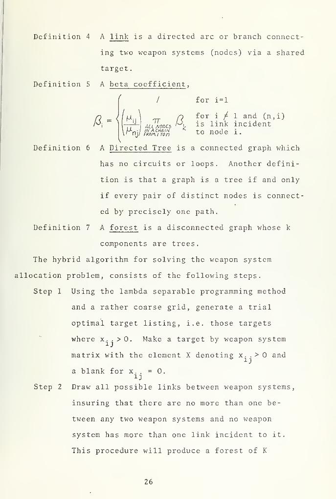
Definition 4 A link is a directed arc or branch connect-

ing two weapon systems (nodes) via a shared

target

.

Definition 5 A beta coefficient,

( I for i = l

»A ir a HWS 1 and (n,i)

— | ALL MODES ' ^ 1S 11T1

le 1

.

A-\

o tor i f 1 and (_n

rr-l /luTLfs H is link incidentMv>w ma chain K tn nnrlf

Definition 6 A Directed Tree is a connected graph which

has no circuits or loops. Another defini-

tion is that a graph is a tree if and only

if every pair of distinct nodes is connect-

ed by precisely one path.

Definition 7 A forest is a disconnected graph whose k

components are trees.

The hybrid algorithm for solving the weapon system

allocation problem, consists of the following steps.

Step 1 Using the lambda separable programming method

and a rather coarse grid, generate a trial

optimal target listing, i.e. those targets

where x. . >0. Make a target by weapon system

matrix with the element X denoting x..>0 and

a blank for x. . = 0.

Step 2 Draw all possible links between weapon systems,

insuring that there are no more than one be-

tween any two weapon systems and no weapon

system has more than one link incident to it.

This procedure will produce a forest of K

26

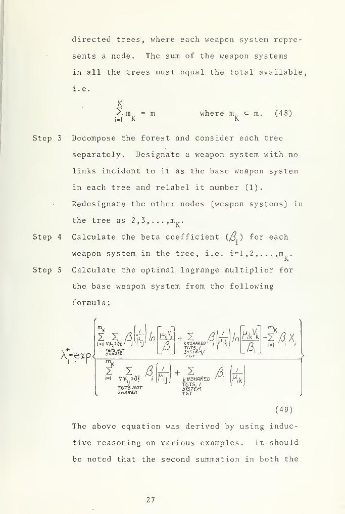
directed trees, where each weapon system repre-

sents a node. The sum of the weapon systems

in all the trees must equal the total available,

i.e.

^ m = mi=l K

where m <^ m. (48)

Step 3 Decompose the forest and consider each tree

separately. Designate a weapon system with no

links incident to it as the base weapon system

in each tree and relabel it number (1)

.

Redesignate the other nodes (weapon systems) in

the tree as 2,3,...,m„.

Step 4 Calculate the beta coefficient {p. ) for each

weapon system in the tree, i.e. i=l,2,...,m .

Step 5 Calculate the optimal lagrange multiplier for

the base weapon system from the following

formula

;

X=eP

Z Z fi\f\lni = i

VL.xJi/ i

lJ 'j'

T6TS /vorSHAPED

UL-.V.r

'J J

4+ 2 ./? rrr \ln

k.V5HARE0'iiPjJc

T&1S,/_' 'J SYSTEM/

TGT

n\B

-Z/2xi i

m,

I X igU+Z & \-L-\

—J! ..-- TGTS, / I /

T6T5 NOTSHARED

SYSTd/<\TGT

(49)

The above equation was derived by using induc-

tive reasoning on various examples. It should

be noted that the second summation in both the

27

numerator and denominator is taken over all

shared targets with the index i representing

only one weapon system per shared target.

Step 6 Calculate A. for all the weapon systems in the

tree from the equation

\ "\^ Cso)

Step 7 Repeat steps 3 through 8 for all the trees in

the forest.

Step 8 Using the Kuhn-Tucker conditions solve for all

the x. .'s by the following formulas.lj

* / /% =IT- i

..V.M..V' 'J J

#X'

and

^SYSTEMSSHARINGTGTj

i

5 fVo/A7M\

where j is notshared (51)

where j is sharedand k is any systemsharing target j

.

(52)

Step 9 Check to see if all remaining Kuhn-Tucker con-

ditions are satisfied. If satisfied, stop. If

not, refine the separable program and repeat

steps 1 through 8.

The hybrid method, like the separable programming

method, has difficulty handling problems whose solution

lies in the tail of the exponential curve. This is caused

by the computer's rounding errors and its inability to dis-

criminate between near zero values. The hybrid method in

its present configuration is incapable of solving problems

28

with lower bounds. However, by rederiving the Kuhn-

Tucker conditions and equation (49) , this method can be

modified to handle the additional constraints. Appendix C

gives applications of the hybrid method to problems of vary

ing sizes.

29

V. EXTENSION OF MODEL AND SOLUTION

The models discussed and used in this thesis are not

inclusive nor necessarily representative of the present

real world situation. Models are constantly changing in

order to reflect current technological and strategic

advances. A model of current interest is one that considers

an allocation of weapons against point and area defenses.

For a recent article addressing this problem, refer to

Miercort, F.A., Soland, R.M. , Optimal Allocation of Missiles

Against Area and Point Defenses [Ref. 11]. Readers interested

in building new models or modifying existing ones should

consult Kooharian, A., Saber, N., and Young, H., A Force

Effectiveness Model With Area Defense of Targets [Ref. 12],

Perkins, F.M., Optimum Weapon Deployment For Nuclear Attack

[Ref. 13] , and Day, R.H. , Allocating Weapons to Target

Complexes By Means of Nonlinear Programming [Ref. 14],

Eckler, A. and Burr A., Mathematical Models of Target Cover-

age and Missiles Allocation [Ref. 15] . For a discussion of

defensive models and methods of solution, the reader is

referred to Dobbie, J.M., On The Allocation of Effort Among

Deterrent Systems [Ref. 16], Brodheim, E., Herzer, I., Russ,

L.M., A General Dynamic Model For Air Defense [Ref. 17],

and Swenson, G.E., Anti-Ballistic Missile Allocations to

Defend Targets With Time Varying Value Structures [Ref. 18].

30

The reader interested in applying and extending the

separable programming technique or the hybrid algorithm to

other models, or models with additional constraints is re-

ferred to Ref. 19 and 20 for additional information on

separable programming.

31

APPENDIX A

The following two examples present an intuitive approach

to Danskin's algorithm. Before proceeding with the examples,

it is necessary to understand the concept of marginal return

(marginal utility) . Marginal return is a measure of the

change in the objective function for a given change in the

independent variable. Symbolically this is expressed as,

Maringal return = ^

'

(A-l)

If we let x be or approximate a continuous variable,

then marginal return becomes,j r

Marginal return = F* = -,— (A-2)

which represents the slope of the objective function at any

given level x. It is assumed that any rational man will

allocate his independent variable so as to maximize (minimize)

his marginal return. With these concepts in mind, examples

1 and 2 are presented.

Example 1

TARGETTARGET WEAPON SYSTEM EFFECTIVENESS VALUE

1 .03 1000

2 .2 100

3 .02 500

4 .2 25

5 .2 10

WEAPONSAVAILABLE 80

Table 1

Parameter Values

32

Step 1 Find the marginal return of the objective

function with respect to the independent

variable (x . ) ; i.e.J

Marginal return = -f^ = ^m e%P \h % \io¥-j J J ' \

J Si

For the above data this yields,

MR (x.

MR (x.

MR (x.

MR (x

MR (x.

= - 30exp(- . 03x,

)

= - 20exp(- . 2x )

= -10exp(-.02x )

= - 5exp(- . 2x .

)

= - 2exp(- . 2x )

Step 2 Since targets with the largest marginal return

are the most attractive and lucrative, the

allocator will fire at those first until his

weapons are exhausted. When all the x.'s are

zero, target one and two have the highest mar-

ginal returns; i.e. -30 and -20 respectively.

Thus the weapons should be allocated to target

1 until its marginal return equals that of

target 2,

-30exp(-.03x ) = -20exp(- . 2(0)) = -20

20expC-.OSx^ =

jq

x1

= 1/.03 ln(1.5) = 13.516

Since x = 13.516 < 80, more weapons can be

allocated.

33

Now targets 1 and 2 are equally attractive

since they both have identical marginal returns,

-20. Therefore, continue to fire at targets 1

and 2 until their marginal return equals the

third highest, target 3,

-30exp(- . 03x ) =- 20exp(- . 2x )=-10exp

x1

= 1/.03 ln(3) = 36.62

-.02(0) = -10

x2

= 1/.2 ln(2) = 3.466

Since x, + x~ = 40. 086 < 80, more weapons can

be allocated.

Now targets 1,2, and 3 are equally attractive

since they all have a marginal return of -10.

Therefore, continue to allocate to targets 1,

2, and 3 until their marginal return equals

the next largest, target 4,

-30exp(- . 03x, )= - 20exp(- . 2x?)= - lOexp (- . 02x.,) =

5exp -.2(0) = -5

Now x-j^ = 59.725

x2

= 6.932

x3

= 34.657.

Since x, + x?

+ x., = 101.314 > 80, weapons can-

not be allocated to targets 1,2 and 3, until

their marginal return is equal to -5. There-

fore, return to the point where their marginal

return equaled -10 (called index L by Danskin)

,

and find a place where their marginal returns

34

are equal and only 80 weapons have been allo-

cated. This will occur for a marginal return

between -10 and -5.

Step 3 Let z be the optimal marginal return between

-10 and -5, and allocate to targets 1,2 and 3

until their marginal return equals -z. Thus,

-SOcrW -.03\ J. +3LU ZOexp-Mz±3te(^-IO^yp\-.02y^

en:p -03j£'\=czp\- I y-'\= eKp\--02^\ =//0 =K

and hence xInK

/.03

xj -- lnK

/.2

x^ =' lnK

/.02.

Regardless of the constant K, where / <: K< / _,

used the same proportion of weapons x', x', and1 2

x' will be used to obtain any marginal return z.

Therefore let K equal .9, and

.1054/ 2

= .5268

X3

= - 1054/.02 = 5 ' 268

Now find the proportions of weapons used

3 513Proportion of x' = q -^ = .3774

Proportion of x* = :5?J = .0566r

2 9.31

Proportion of x* = • 5^ = .566

35

There are 80-40.086 = 39.914 weapons remaining

to be allocated. Of the unallocated weapons

37.71 belong to xj, 5.57% belong to x£,

and 56.6% belong to x'. Therefore the optimal

allocations are

xx

= 36.62 + .377(39.914) = 51.684

x2

= 3.4658 + .0567(39.914) = 5.7248

x3

= + .567(39.914) = 22.591.

Example 2

TARGET WEAPON SYSTEM1

EFFECTIVENESS2

TARGETVALUE

1 .03 .005 1000

2 .2 .2 100

3 .02 .06 500

4 .2 2.0 25

5 .2 .2 10

WEAPONSAVAILABLE

80 50

Table IIParameter Values

Step 1 Calculate the marginal return of the objec-

tive function with respect to the independent

variable (x..)« For the above data, this givesi]

MR(xn ) = -30exp [-(.03xi;L

+ .005x21 )]

MR(x-,2 )

= -20exp - (. 2x-, 9+ '^ x

22t

MR(x13 ) = -lOexp ['(•02x

13+ .O6X23)]

MR(x14 ) = -5exp £(.2x

14+ 2x

24 )]

36

MR (x15

)= -2exp[-(.2x

15+ .2x

25 )]

MR(xn )« -5exp[-(.03xn + .005x

21 )j

MR(x22 )

= -20exp [- (. 2x, 2+ .2x

22 )

MR(x23 )

= -30exp [-(.02x + • 06x2 3

)]

MR(x24 )

= -50exp [(.2x14

+ 2x24 )]

MR(x ) = -2exp[-(.2x + . 2x )

25 L 15 25-1

Step 2 Allocate weapon system 1 to the 5 targets.

The solution of example 1 gives the needed solu-

tion. Weapons are allocated to targets 1,2,

and 3 until their marginal return was -6.365.

The allocation was

x = 51.678

x,2

= 5. 724

x, , = 22 . 586.

Because of this allocation the marginal returns

are adjusted as follows,

MR(x

MR(x

MR(x

MR(x

MR(x

MR(x21

MR(x22

MR(x23

MR(x

11

12

13

14

15

MR(x

24

25

= -6.365exp(-.005x )

— X

= -6 . 365exp (- . 2x )F22

= -6 . 365exp(- . 06x )

= -5exp(-2x24

)

= - 2exp (- . 2x2r)

= -1.061exp(- .005x21 )

= -6 . 365exp (- . 2x )

= -19.095exp(-.06x )

= -50exp(-2x24

)

= -2exp(-.2x25

)

.

37

Step 3 Progress through the target list allocating

x?

to the targets with the largest marginal

return, as previously discussed, until the

problem is solved without a shared target or

until a shared target is encountered. Hence

allocate to target 4 until its marginal return

equals the next highest, target 3,

50exp(-2x24 ) = -19.095exp .06(0) 19.095,

x24

= .4797.

There are 49.5203 weapons of type 2 unallocated,

and target 3 has the next highest marginal

return. Since target 3 already has weapons of

type 1 allocated, there is a possibility of a

shared target.

Step 4 Target 3 will have weapons of type 2 allocated

to it regardless of whether or not it receives

weapons of type 1. Therefore remove target 3

from x's target list and check to see if in

fact it is shared. Adjusting the marginal

returns to reflect the weapons of type 2 already

allocated yields

MR(x

MR(x

MR(x

MR(x

MR(x

MR(x

11

12

14

15

21

22

= -30exp(-.03x )

= -20exp(-.2x )

= -1.9095exp(-.2x )F ^ 14

= -2exp(-.2x )

= -5exp[-(.03x + .005x21 )J

20exp[j

(. 2x + . 2x2 2)|

38

MR-T&

2X o )]25J

:(x23 ) = -30exp [-(-0 2x

13

MR(x24 ) = -19.095exp[-(.2x

14 )|

MR(x25

) = -2exp £(.2x

Allocate weapon system 1 according to the newly-

calculated marginal returns. As a result

weapons will be allocated to targets 1 and 2

until their marginal returns equal -3.514,

x = 71.492

x = 8.694.

Adjusting the marginal returns to reflect the

above allocation yields,

MR(x

MR(x

MR(x

MR(x

MR(x

MR(x

MR(x

MR(x

MR(x

11

12

14

15

21

22

23

24

25

= -3.514exp(-.005x„ )F21

= - 3 . 514exp (- . 2x )

= -1.9095exp(-2x )

= -2exp(-.2x25

)

= - .586exp(- .005x )

= -3. 514exp(-2x )

= -30exp(-.06x )

23

= -19.095exp(-2x )

= -.2exp(-.2x ) .

Step 5 Continue the allocation of weapon system 2

to the target list. Recall that target 4 has

.4797 weapons previously allocated. Allocate

to target 3 until its marginal return equals

-19.095.

-30exp(-.06x ) = -19.095

39

x =7.6 24 and23

x, + x < X24 23 2

The marginal return for target 3 and weapon

system 2 is now -6 . 33exp(- . 02x ). Target 3

is still possibly shared since -6.33 is a larger

marginal return than -3.514.

Step 6 Continue allocating weapon system 2 until the

marginal return of target 3 and 4 is equal to

the next largest, -3.514,

-50exp(-2x ) = -30exp(-.06x ) = -3.514,

thus

x?

= 35. 726

X24 = 1.328 and

X23

+ X24<X 2-

The marginal return of weapon system 1 against

target 3 is now,

- lOexpL

02x + .06(35.726) 1.176exp(- .02x15 )

Since the marginal return - 1 . 176exp (-. 02x )<

-3. 514exp(- . 02x, ,) , target 3 will not be shared

in the optimal allocation. Continue allocating

weapon system 2 to the target list. Target

2, which is the next largest marginal return has

weapons of type 1 already allocated. Hence

there is a possibility of a shared target.

Step 7 Repeat steps 4 through 6 using target 2. Delete

target 2 from weapon system l's target list and

40

allocate to remaining targets. Adjusting the

marginal returns to reflect weapon system 2's

current al

MR(x

MR(x

MR(x

MR(x

MR(x

MR(x

MR(x

MR(x

MR(x

11

13

14

15

21

22

23

24

25

ocation yields,

= -30exp (.03x + .005x2i

)

1. 176exp -(.02x .06x23 )

. 33514exp -(.2x + 2x114 24

J

2exp

= -5exp

= -20exp

(.2x15

+ .2x25

)

(.03XJ. + .005x21 )

C.2x12

.2x22

)

3. 514exp

= -3.514exp

-(.02x13

+ .06x )

(•2x14

+ 2x24 )

2exp (.2x15

.2x25

)

As a result all 80 weapons can be allocated to

target 1 until its marginal return equals

-2.72exp(- .005x2

) .

Step 8 Adjust the marginal returns to reflect this

current weapon system 1 allocation,

MR(x1;L

) = -2.72exp

MR(x13

) = -1.176exp

MR(xn ) = -.3514exp14

(.03x + .005x21 )

(.02x + .06x 77 )23-

-(.2x + 2x )

14 24

41

MR(x

MR(x

MR(x

MR(x

MR(x

15

21

22

23

24

2exp (.2x15

.2x )

. 453exp (.03x + .005x21 )

= -20exp -(.2x .2x22

)

3. 514exp

3. 514exp

-(.02x .06x23

)

-(.2x14

+ 2x24 )

MR(x2 r) = -2exp (.2x n

+ .2x )15 25

Allocate weapon system 2 to target 2 until its

marginal return equals -3.514. As a result

x ~ = 3.7 and x ~ + x„_ + x_„<X„. Thus, more22 22 23 24 2

weapons can be allocated to targets 2,3, and 4

until their marginal return equals the next

largest, -2. Weapons can only be allocated

until their marginal returns equal -2.886

with

x22

= 9.66

x23

= 39.4

x24

= 1.32.

Step 9 Recalculate weapon system l's marginal return

for this current allocation. As a result

MR(x ) = -2.8886exp(-.2x12

)

.

Since marginal return of - 2 . 886 > - 2 . 72 , target

2 will be shared. Hence, the optimal solution

for weapon system 1 is allocation to targets 1

42

and 2, and weapon system 2 is allocation to

targets 2, 3, and 4.

Step 10 The optimal marginal returns (A and A?

) can

be calculated from equation (49) , and the

following solution can be obtained.

TARGETSWEAPON

1

SYSTEM2

1 79.132

2 .868 8.992

3 39.556

4 1.442

5

Table IIIWeapon Allocation Solution

43

APPENDIX B

The following two examples illustrate solutions by the

separable programming method. Both solutions were obtained

using the nesting refinement method.

Example 1

. TARGETSWEAPONS SYSTEM

EFFECTIVENESS: ^ijTARGETVALUE

1 .10 1000

2 .02 500

3 .05 200

4 .08 100

5 .01 500

WEAPONSAVAILABLE 50

Table IVValue of Parameters

TARGETSGRID

SIZE 25.

GRIDSIZE 5

GRIDSIZE 5

GRIDSIZE 10

EXACTSOLUTION

1

2

3

4

5

25.999

15.999

6.0

2.00

26.399

15.6001

6.399

1.60001

26.239

16.08

6.559

1.12001

26.239

16.08

6.432

1.248

26.2436

16.0883

6.4353

1.2328

Table VWeapon Assignment: X

!J

44

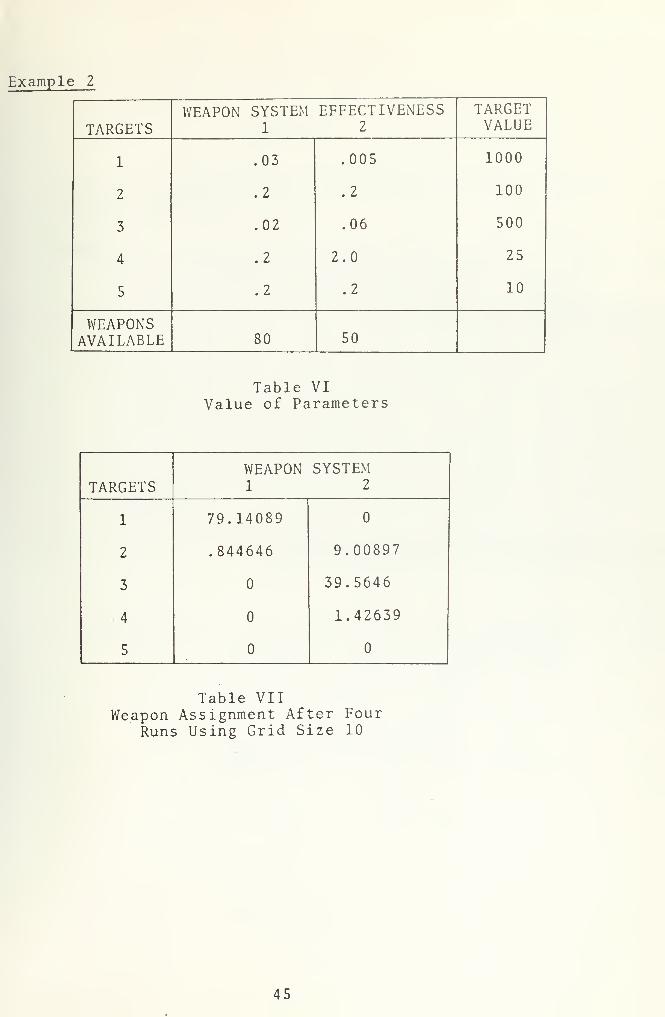
Example 2

TARGETSWEAPON SYSTEM

1

EFFECTIVENESS2

TARGETVALUE

1 .03 .005 1000

2 .2 .2 100

3 .02 .06 500

4 .2 2.0 25

5 .2 .2 10

WEAPONSAVAILABLE 80 50

Table VIValue of Parameters

TARGETSWEAPON SYSTEM1 2

1

2

3

4

5

79.14089

.844646 9.00897

39.5646

1.42639

Table VIIWeapon Assignment After Four

Runs Using Grid Size 10

45

APPENDIX C

The following three examples illustrate solutions obtained

by the hybrid algorithm.

Example 1

TARGETSWEAPON SYSTEM EFFECTIVENESS12 3

TARGETVALUE

1 1 5 3 1

2 2 4 4 1

3 3 3 5 1

4 4 2 4 1

5 5 1 3 1

WEAPONSAVAILABLE 1 1 1

Table VIIIValue of Parameters

Step 1 Use the separable program with a grid equal

to. 10, to obtain a target by weapon system

matrix. Draw all possible links.

WEAPON SYSTEMTARGET 12 3

1

2

3

4

X

AS " A

X

X > X

5 X

46

Step 2 Calculate all beta coefficients.

A4 -

Step 3 Calculate \

4. U

4.

4

= 1

= 1

X*= eyp

/n(5) + (/)ln(5) + ln(5) i- In (4) + /nM5 5 5 4 4

-/-/-/

5 5 5 4- 4

X = .29544

Step 4 Calculate all X.'s,

X* = X* = .29544.

Step 5 Using the Kuhn-Tucker conditions calculate

the optimal allocation, and insure that all

the Kuhn-Tucker conditions are satisfied.

TARGETWEAPON

1

SYSTEM2

ALLOCATION3

1 .56514

2 .43426 .21713

3 .56514

4 .43426 .21713

5 .56514

Table IXSolution Matrix

47

Example 2

TARGETSWEAPON SYSTEM EFFECTIVENESS12 3 4

TARGETVALUE

1

2

3

4

5

6

.01

.001

.02

.015

.1

.07

.075

.01

.02

.013

.019

.02

.015

.1

.01

.03

.04

.05

.1

.01

.02

.02

.1

.01

500

900

700

300

600

100

WEAPONSAVAILABLE 20 25 50 15

Table XValue of Parameters

TARGETSWEAPON SYSTEM ALLOCATION12 3 4

1

2

3

4

5

6

.373

19.627

25

29.14

20.3

.48

15

/S! 1 1 notshared

notshared

Table XISolution Matrix After 3 Separable

Nesting Runs Using Grids of5, 5, and 5 Respectively.

48

Example 3

TARGETWEAPON ,

1 2

SYSTEM3

EFFECTIVENESS4 5 6

TARGETVALUE

1 .4 .5 .1 .27 .33 .41 100

2 1.0 .3 .31 .4 .8 .7 250

3 .8 .2 .51 .7 .3 .6 600

4 .2 .3 .4 .75 .6 .25 200

5 .9 .2 .17 .28 .4 .5 300

6 .5 .1 .15 .2 .3 .4 100

7 .1 .2 .23 .18 .24 .4 450

8 .6 .43 .5 .1 .02 .38 500

9 .6 .1 .4 .3 .2 .6 800

10 .2 .33 .3 .4 .53 .5 900

WEAPONSAVAILABLE 10 20 15 5 10 15

Table XIIValue of Parameters

49

TARGETWEAPON SYSTEM ALLOCATION12 3 4 5 6

1

2

3

4

5

6

7

8

9

10

.6601

4.5381

4.7958

6.1897

8.3803

5.430

9.2657

1.8999

3.8239

.032

4.9679

4.18

5.82

9.5487

5.4512

. . . - . .- .i

2.008 1 1.1628 1.596 1.606 1.744

Table XIIISolution Matrix After Separable

Run Using Grid Size 10.

50

WEAPON SYSTEM ALLOCATICN PROBLEMCOEFFICIENT GENERATOR FOR THELAMBDA METHOD SEPARABLE PROGRAM

CCCc

THIS PROGRAM IS DESIGNED TO BE USED IN CONJUCTIONWITH THE SEPARABLE PROGRAMMING METHOD OR THEHYBRID ALGORITHM AS DESCRIBED IN SECTION III PARTB AND C RESPECTIVELY,

DEMENSICN STATEMENTS

Ccccccccc

THIS PROGRAM HAS BEEN DIMENSIONED FOR A MAXIMUM OF 6WEAPON SYSTEMS, 20 TARGETS, AND A GRID SIZE OF 100.DIMENSION STATEMENTS MUST BE CHANGED FOR LARGERPROBLEMS. THE DIMENSION OF ANSMAT IS CHANGED ASFOLLOWS:

NUMBER OF ROWS = (3-NUMEER OF TARGETS )+( NUMBER OFTARGETS*NUMBER OF WEAPON SYSTEMS)+( NUMBER OF WEAPON SYSTEMS + 1)

NUMBER OP COLUMNS = GRID SIZE + 1

VAL( 20), EFFECT(6,20) ,UPPERX(6) ,UPPERY(20)V.'PNTGT(20 ), ANSMAT 1159, 101),UPSOLN(6,20),

DIMENSION2 BLOWY (2 0)3BOTSOL(6,20) ,U?OLD(6,20),6LOLDX(6,20),SOLN16,20)

INPUT DATA CARDS

CCCCCCCcCCcccccccc

INPUT DATA CA-Tc

THE FOLLOWINGCARD SET l:

CARD SET 2:CARD SET 3:

CARD SET 4:

CARD SET 5:

CARD SET 6:CARD SET 7:CARD SET 8:

CARD SET 9:

CARD SET 10:

DS WILLCRCER:N=NUMBN=NUMBVAL(K)EFFECTSYSTEMUPPERXWEAPONWPMTGTMUST BCELTA=SOLMJUPCLC (

PREVIOBLOLDXOF PREGRID S

BE READ INTO THE PROGRAM IN

ERER= VAL( J,KJ AU) =

SYS(K) =

E USGRID,K) =

J,K)US s(J,KVIOUIZE

FFUE)=

GAAVTENUED

PR= UOL)=

SOF

WE ATAPOF

E C FINSAILM JMB c

AGIZEEVIPPEUTILOWSOLPR

PON SYSTEMSGETSTARGET KECTIVENESS CF WEAPONT TARGET KABLE STOCKPILE OF

P OF TOTAL WEAPONS THATAINST TARGET K

OUS ALLOCATION SOLUTIONR LIMIT ON THE RANGE OFONER LIMIT ON THE RANGEUTIONEVIOUS RUN

READ IN THE NUMBER OF WEAPON SYSTEMS AND TARGETS

READ (5,1003)M,N1000 FORMAT (2110)

51

C READ IN TARGET VALUES, WEAPON SYSTEM EFFECTIVENESS,C AVAILABLE STOCKPILE, AND TOTAL WEAPONS TO BE USEDC AGAINST TARGET K.C NOTE: WPNTGT(K) MUST BE ZERO IF USING THE HYBRIDC ALGORITHM

READ (5,1100) (VAL(K) ,K=1,N)READ (5,1130) ( (EFFECT(J,K),K=1,N) , J=1,M)READ (5,1100) (UPPERXl J) ,J = 1 ,M)READ(5,1100) ( WPNTGTIK ) ,K=1,N)

1100 F0RMAT(13F7.3)

C READ IN GRID SIZE TO BE USED

READ ( 5, 12C0JDELTA1200 FCRMAT(F7.1)

C READ IN PREVIOUS SOLUTION, AND ITS UPPER AND LOWERC RANGES.C NOTE: FCR GRID REFINEMENT METHOD USE SOLN=MID-RANGEC OF WEAPONS AVAILABLE, UPCLD=UPPER LIMIT ONC STOCKPILE, ANC BLCLCX=ZERO ON ALL RUNS.C FOR THE NESTING REFINEMENT USE THE SAME DATA ASC THE GRID REFINEMENT FOR THE FIRST RUN. ON ALLC SUCEEDING RUNS USE THE ACTUAL SOLUTICN FORC SCLN, AND THE UPPER AND LOWER RANGES OF WEAPONC SYSTEM J AGAINST TARGET K FROM THE COMPUTERC PRINT OUT.

READ (5,1130) ( (SOLN(J ,K) ,K=1,N), J=1,M)RFAD (5,1100) ( ( UPOLDt J ,K) ,K=1,N) , J = 1,M)READ (5.1100) ( (BLCLDX( J,K),K=1,N), J=1,M)

C READ IN PREVIOUS GRID SIZEC NOTE: WHEN USING THE GRID REFINEMENT METHOD ALWAYSC READ IN 0LDELT=2. WHEN USING THE NESTINGC REFINEMENT METHOD READ IN 0LDELT=2 FOR THEC FIRST RUN AND USE THE GRID SIZE FROM THEC PRECEEDING RUN FOR EACH SUCEEDING RUN.

READ (5,1200) OLCELT

C PRINT OUT SOME PARAMETERS THAT WERE REAC INTO THEC PROGRAM AND CALCULATE THE NEW RANGES FOR THEC FUNCTION GI JK(Y(K)

)

C PRINT OUT THE NUMBER OF TARGETS AND WEAPON SYSTEMS

WRITE (6, 1010)M,N1010 FCRMATC 1' ,' WEAPON SYSTEMS = ' , I 5 ,/ , IX , »T ARGETS= • , I 5, / )

C PRINT CUT THE TARGET VALUE

DO 3 K=1,NWRITEC6 ,1113)K,VAL(K)

1110 FORMAT! IX, 'VALUE OF T ARGET • , I 3 ,2X ,• =» , ^1 .3 )

3 CONTINUE

52

C PRINT OUT WEAPON SYSTEM EFFECTIVENESS AND CALCULATEC RANGES FOR GI JK(Y(K) )

DO 5 J = 1,MDO 4 K = l ,NY=(UPGLD U,K)-3LCLDX{J,K))/OLDELTUPSOLNC J,K)=SOLN(J,K)+YBOTSOL( J ,K) =SDLN( J,K)-YIF(BOTSOL( J,K) .GE.O.O) GO TO 112BCTSOL(J,K)=0.0

112 IF(UPSOLN( J,K) .LE. UPPERX(J) ) GO TO 11UPSOLNl J,K )=UPPERX( J

)

11 WPITE(6,112 0)J , K, EFFECT ( J, K)1120 FORMAT! IX, 'EFFECTIVENESS OF WEAPON SYSTEM' ,1 5 ,3X

,

2« AGAINST TARGET' ,I5,2X,»=',F8.5)4 CONTINUE5 CONTINUE

PRINT OUT WEAPON SYSTEM STOCKPILE

DO 6 J = 1,MWRITE(6,1130)J,UPPERX(J)

1130 FCRMATdX, 'UPPER LIMIT OF WEAPONS OF TYPE', 15, 3X,2' AVAILABLE=' ,F8.3)

6 CONTINUE

PRINT OUT TOTAL WEAPONS TO BE USED AGAINST TARGET K

DO 7 K=1,NWRITE16, 1135)K,WPNTGT(K)

1135 FCRMATdX, ' LOWER LIMIT OF WEAPONS TO BE USED AGAINST2TARGET' ,1X,I5,1X,'=',F10.5)

7 CONTINUE

PRINT GUT GRID SIZE

WRITE! 6, 1140)DELTA1140 FORMATdX, 'NUMBER OF I NT ER V A LS = ' , F 3 . 3

)

CALCULATE PARAMETERS FOR DO LOOPS

KK=N+MNN=(M+1 )*NMM=(M+N+1)+ (M+l )*NKNM=MM+NKKNN=KK+NN

53

PREPARE THE FIRST SET OF CARDS c OR THE VPS SYSTEM

CARDS THAT DEFINE TYPE OF CONSTRAINT

1500

710

7157G3

15 30

73315 40

7251545720

1510

7501520

7451525740

1546

7701547

7751548780

1550

WRITE(7,FORMAT (

DO 70 I

IFU.GT.IFU.GT.WRITE( 7,GO TO 70WRITE (7,GO TO 70W R I T E ( 7 ,

CONTINUEDO 720 JJV=J+NI F ( J M . G TIFfJM.GTWRITE(7,FORMAT < 1

GO TO 72WRITE(7,FORMAT ( 1

GO TO 72WRITE( 7,FORM AT ( 1

CONTINUEDO 740 JJN=J+KKIF( JN.GTIF{ JN.GTWRITE(7,FGRMATI1GO TO 74WRITEC7,FORMAT(

1

GO TO 74WRITE (7,FORMAT { 1

CENT INUEDO 780 KJO=KKNN+IF( JO.GTIF(JO.GTWRITE(7,FORMAT (1GO TO 78WRITE{7,FORMAT (1GO TO 73WRITE(7,FORMAT (1CONTINUEWRITE(7.FORM ATP

15C0)ROrtS» »/ t IX, «N» ,2X, 'C )

= 1,N99) GO TO 7159} GO TO 7101510)1

1523)1

1525 )I

= 1,M

.99) G

.9 ) GO1530JJX «L' ,

1543JJMX, 'L' ,2X, 'R' ,12)

1545) JMX, !_' ,2X, «R«, I 3)

TO 725TO 730

M2X, «R« ,1 1)

= 1,NN

.99) G

.9) GO1510)JX.' E' ,

C1520)JX,'E'

1525 )JX,'E« ,2X,« R' ,13)

TO 745TO 750

N2X,' R» , II )

N2X,« R« ,12)

N

= 1,NK.99 ) G.9) GO1546)JX, •

G' ,

1547)JX, 'G« ,

1548JJX,' G' ,

1550)COLUMN

TO 775TO 773

2X,'R', II)

32X, 'R', 12)

2X,» R» , 13)

S' )

CALCULATE THE NUMBER OF MESH POINTS

NDELTA=DELTA+1

54

START THE MAIN DC LOOP FOR CALCULATING COEFFICIENTS

DO 200 K=1,NN

C INITIALIZE THE MATRIX FOR STORING THE COEFFICIENTSC BY SETTING IT EQUAL TO ZERO

DC 10 T I=1,NDELTADO 10 LL=1,KNMANSMATJLL, II )=0.0

10 CCNTTNUE

C CALCULATE THE UPPER LIMIT FOR THE FUNCTICN FIKIYCK))C WHERE K=1,2,...,N

IF(K.GT.N) GO TO 31OLDROT=0.0OLDUP=0.CO 20 JJ=1,MUPPERY(K)=EFFECT(JJ,K)*UPSOLN( JJ.K)+OLDUPBLOWY (K)=EFFECT( J J , K) *30TS0L ( J J , K) +CLDBOTCLDUP=UPPERY(K )

0LCB0T=3L0WY(K)20 CONTINUE

RY=(UPPERY(K)-BLCWY(K))/DELTACLOWY=BLOWY(K)

C CALCULATE THE COEFFICIENTS FOR THE FUNCTICN FIK(Y(K)}C WHERE K = l,2 N

DO 30 MA=1,NDELTAANSMAT( 1,MA)=VAL(K)*EXP(-CL0WY)CLOWY=CLCWY+RY

30 CONTINUE31 CONTINUE

Cc

CALCULATE THE COEFFICIENTSGIJK(Y(K)) WHERE J=l,2t.

FGR THE FUNCTICN.» (M+M)

DO 100 J=lIF(J.GT.N)IF(J.EQ.K)GO TO 38

KKGO TOGO TO

7035

C CALCULATE THE COEFFICIENTSC WHERE J=l,2 N ANC K = J

35 KA=K+1CO 40 M3=1.NDELTAANSMAT(KA,M3)=3L0WY(K)BLOWY! K)=BLOWY(K)+RY

40 CCNT INUEGO TO 1J0

FOR THE FUNCTION GIJK(Y(K))

C CALCULATE THE COEFFICIENTS FORC WHERE J=lf2i....N t K =M + J, AND

THE FUNCTIONI=li2 i... »N

GIJK{ Y(K))

38 CO 60 1=1,

M

KB=(N*I )+JIFCK.NE..KS) GO TO 6RX=(UPSOLN(I,J)-SOTSCL(I,JJJ/DELTACLOWX=BOTS£L(I J)

55

JA=J+1DO 50 MC=1,NDELTAANSMATt JA,MC}=(-EFFECT(ICLOWX=CLOWX+RX

50 CCNTINUE60 CONTINUE

GO TO 10070 CCNTINUE

J) )*CLOWX

Cccc

CALCULATE THE COEFFICIENTS FOR THE FUNCTION GIJK(Y(K))WHERE J=lN+l,N+2«... »N+M, J=N(J-N)+1, AND L=1,2»...N;ANC THE COEFFICIENTSCONSTRAINT

FOR THE TOTAL WEAPONS PER TARGET

CO 9 L = 1,NKD=(N*( J-N) J+LIF(K.NE.KD) GO TO 90LL=J-NLA=J+1LR=f'M+LRZ=(UPSOLN( LL,L)-BOTSOL(LL,L) ) /DELTADLOWX=8OTS0L(LL,LJDO 8 MD=1.NDELTAANSMAT(LA,MD)=DLOWXANSMAT(L3,MD)=DL0WXWRITE(6,1145)DL0WX

1145 F0RMAT(80X,F12.6)DLOWX=DLCWX+RZ

80 CONTINUE90 CCNTINUE

100 CCNTINUE

c CALCULATE THE COEFFICIENTS FOR THEc EQUAL 1 CONSTRAINT

SUM OF THE LAMBDAS

ME=M+N+l+KCO 110 LA=1,NDELTAANSMAT(ME,LA)=1.0

110 CCNTINUE

56

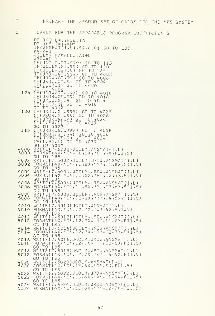
PREPARE THE SECOND SET CF CARDS FOR THE MPS SYSTEM

CARDS FOR THE SEPARABLE PROGRAM COEFFICIENTS

DO 193 L=1,NDEDO 18 5 I = 1 , K NMIF( ANSMAT1 1,1)KA=K-1JCOLM=(KA*NCELJROW=I-lIF(JC0LM.GT.99IF( JCOLM.GT .99IF( JCOLM.GT. 9)IF(JR0W.GT.999IF( JR0W.GT.99)IF( JR0W.GT.9)IF(I.EO.l) GOGO TO 4002

125 IF{ JR0W.GT.999IF( JR0W.GT.99)IF( JR0W.GT.9)IF(I.EO.l) GOGO TO 4012

120 IFUR0W.GT.999IFUR0W.GT.99)IF( JR0W.GT.9 }

IF(I.EO.l) GOGO TO 4022

115 IFUR0W.GT.999IF( JR0W.GT.99)IF( JR0W.GT.9 )

IF(I.EQ.l) GOGO TO 4032

4000 WRITE(7,5000)J5000 FCRMAT(4X,' C

,

GO TO 1854002 WRITE(7,5002 )J5002 F0RMAT(4X.'C ,

GO TO 18540 04 WRITE (7 ,50 04)

J

5004 FORMAT! 4X, 'C ,

GO TO 1854006 WRITE17 ,5006)

J

5006 FORMAT! 4X, 'C ,

GO TO 1854008 WRITE(7,5008) J5008 F0RMAT14X, 'C ,

GO TO 1854010 WRITE! 7,501 JJJ5010 FORMAT ( 4X, 'C ,

GO TO 1854012 WRITE! 7,5012)

J

5012 F0RMVM4X. , C«.GO TO 185

4014 WRITE!7,5014)

J

5014 FORMAT (4X, 'CGC TO 185

4016 WRITE(7,5016)J5016 FORMAT (4X. 'C ,

GO TO 1854018 WRITE(7, 5018)J5018 F0RMAT!4X, »C» ,

GO TO 1854020 WRITE(7, 5020)J5020 FORMAT !4X, ' C ,

GO TO 1854022 WRITE(7. 5022JJ5022 FORMAT ( 4 X,' C

,

GO TO 1854024 WRITEI7, 5024)J5 024 FCRMAT(4X,' C ,

LTA

.EC. 0.0) GO TO 185

TA)+L

9) GO TO 115) GO TO 120GC TO 125

) GO TO 4008GO TO 4006

GO TO 4004TO 40C0

) GO TO 4018GG TO 4016

GO TO 4014TO 4010

) GC TO 4028GO TO 4026

GO TO 4024TO 4020

) GO TO 4038GO TO 4036

GO TO 4034TO 4030

COLM,ANSMAT( I ,L)II ,3X,'C ,9X,F11.5)

COLM, J ROMAN'S MAT! I,L)II ,8X,«R« ,11 ,8X,F11.5)

COLM, JROW,ANSMAT( I,L

)

I l,8Xt 'R' ,I2,7X,F11.5)

CCLM, JROW,ANSMAT ( I,L)I 1 , 8 X , ' R «,I3,6X,F11. 5)

COLN, J ^CW, AIMS MAT { I ,L)I1,3X,»R',I4,5X,F11.5)

CCLM,ANSMAT(I ,L)12, 7X, «C • ,9X,F11. 5)

CCLM, JPQW,ANSMAT{ I,L)12, 7X, «R«,I 1,8X,F11.5)

CCLM, JFOW,A,NSMAT(I ,L)I2,7X,«R« ,I2,7X,F11.5)

COLM, JROW,ANSMAT(I ,L)12, 7X, »R», I3,6X,F11.5)

COLM, JROW*ANSMAT( I ,L)12, 7X, 'R J

, 14, 5X, F11.5)

COLM,ANSMAT{ I ,L)13, 6X, 'C* ,9X,F11 .5)

COLM, JROW,ANSMAT( I ,L)I3,6X,'R« , U,8X,F11.5)

COLM, JRCW,ANSMAT{ I ,L)I3,6X,'R' ,I2,7X,F11.5)

57

40265026

40285028

40305030

40325032

4034

40365036

403850381851902 00

GO TG 18WRITE!7,F0RMAT(4GO TO 18WRITEC7 ,

F0RMAT14GO TO 18WRITF (7 ,

FORMAT (4GC TO 18WRITE17,FORMAT (4GO TO 18WRITE(7,FORMAT (4GC TO 18WRITE! 7,FORMAT (4GO TO 18WRITE (7,FORMAT (4CONTINUECONTINUECCNT INUE

550 2 6X,'C55028X,'C5

5030X, »c55032X, «C55334X, 'C

5036X, «C55038X, «C

JJCOLM,• , 13, 6X

) J C C L M ,

• ,13, 6X

JFOW,ANSMAT(,« R r ,I3,6X,F

JRCW,ANSMAT(,'R« ,I4,5X,F

) JCCLM, ANSMAT! I,L):,'C ,9X,F11.1

, 14, 5X

) JCCLM,», 14, 5X

) JCCLM,• , 14, 5X

) JCCLM,', 14, 5X

JJCOLM,', 14, 5X

JRCW,ANSMAT (

, 'R' ,I1,8X,F

JRCW,ANSMAT!, »R» ,I2,7X,F

JPOW,ANSMAT(, «R« , I3,6X,F

JROW,ANSMAT(, «R» ,I4,5X,F

I,L)11.5)

I,L)11.5)

5)

I ,L)11*5)

I,L)11.5)

I,L)11.5)

I ,L)11.5)

CARDS FOR THE RIGHT HAND SIDE OF THE CONSTRAINTS

6000

6010

70206020300

6030

70406040

70506050350

7070

708060804C0

WRITE17,FORMAT!

•

DO 300 I

JRHS=IRHIF( JRHS.WRITE ( 7,FORMAT (4GO TO 30WRITE! 7,FORMAT !4CONTINUECO 350 LKRHS=KK+IF! KRHS.IFIKRHS.WRIT- (7,FORMAT!

4

GC TO 35WRITE!7,FORMAT (4GO TO 35WRITE! 7.FORMAT!

4

CCNT INUEDO 400 MNRHS=MRHIFtNRHS.IF(NRHS.WRITE!7,GO TO 40WRITE (7,GC TO 40WRITE! 7,FORMAT (4CONTINUESTOPEND

6000RHS'RHS =

S+NGT.96010X,' B

602CX, »B

RHS =

LRHSGT.9GT.96030X, «B

6040X, '3

6053X, «3

)

)

1,M

) GO)JRH' ,9X

)JRH' ,9X

1,NN

9) G) GOJKRH• ,9X

TO 7020S,UPPERX(IRHS)t»R , tIlf8Xf.F11.5J

S,UPPERX(IRHS),'R 1

, I2,7X,F11.5)

C TO 7C50TO 7040

S,'R' ,1 1,13X, 'l.O'l

1 K RHS' ,9X>R« ,I2,12X, »1.0« )

)K?H' ,9X ,'R',I3,11X, 1.0«

)

RHS=1,NS+KKNNGT.99) GGT.9) GO6010JNRH36 02 0)NRHS,WPNTGT(MRHS)

6080JNRHX, 'B' ,9X

TO 7080TO 7070

S, WPNTGT(MRHS)

S, WPNTGT(MRHS),'R ' ,I3,6X,F11.5)

58

LIST OF REFERENCES

1. U.S. National Defense Research Committee OperationsEvaluation Group Report No. 56, Theoretical BasisFor Methods of Search and Screenin g, by B. 0.Koopman, v. 2B, p. 45-46, 1946.

2. Danskin, J. M. , The Theory of Max-Min , p. 85-106,Springer-Verlan, 1967.

3. denBroeder, G. G., Ellison, R. E., and Emerling, L.,"On Optimum Target Assignments," Operations Research

,

v. 7, p. 322-326, May-June 1959.

4. Mylander, C. W. , "Applied Mathematical Programming,"Proceedings of the United States Army OperationsResearch Symposium , 4th, 1965, part 1, p. 99-110,March-April 1965.

5. Lemus, F. and David, K. H. , "An Optimum Allocation ofDifferent Weapons to a Target Complex," OperationsResearch , v. 10, p. 787-794, September-October 1963.

6. Hadley, G., Nonlinear and Dynamic Programming, p. 104-

147 and p. 190-202, Addison-Wesley , 1964?

7. Hillier, F. and Lieberman, G. J., Introduction to Opera -

tions Research, p. 574-594, Holden-Day, 1970

.

8. Passy, U., "Nonlinear Assignment Problems Treated ByGeometric Programming," Operations Research, v. 19,p. 1675-1690, November-December 1971.

9. Manne, A. S., "A Target-Assignment Problem,", OperationsResearch , v. 6, p. 346-551, May -June 19 58.

10. Amerault, J. F., A Computerized Algorithm , M. S. Thesis,U.S. Naval Postgraduate School, Monterey, Californa,1972.

11. Miercort, F. A. and Soland, R. M. , "Optimal Allocationof Missiles Against Area and Point Defenses," Opera -

tions Research , v. 19, p. 605-617, May-June 1971.

12. Kooharian, A., Saber, N., and Young, H. , "A Force Effec-tiveness Model With Area Defense," Operations Research ,

v. 17, p. 895-906, September-October 1969.

59

13. Perkins, F. M. , "Optimum Weapon Deployment For NuclearAttack," Operations Research , v. 19, p. 77-94,January-February 1961.

14. Day, R. H. , "Allocating Weapons To Target Complexes ByMeans of Nonlinear Programming," Operations Research ,

v. 14, p. 992-1015, November-December 1966.

15. Eckler, A. R. and Burr, S. A., Mathematical Models ofTarget Coverage and Missile Allocation , MilitaryOperations Research Society, 1972.

16. Dobbie, J. M. , "On the Allocation of Effort AmongDeterrent Systems," Operations Research , v. 7,

p. 335-346, May-June 1959.

17. Brodheim, E., Herzer, I., and Russ, L. M. , "GeneralDynamic Model For Air Defense," Operations Research

,

v. 15, p. 779-796, September-October 1967.

18. Kentron Hawaii, Ltd., Anti-Ballistic Missile AllocationTo Defend Targets With Time Varying Value Structures

,

by G. E. Swinson.

19. Charnes, A. and Lemke, C. E., "Minimization of NonlinearSeparable Convex Functions," Naval Research LogisticsQuarterly , v. 1, p. 301-312, December 19 54.

20. Alloin, G. "A Simplex Method for a Class of NonconvexSeparable Problems," Management Science , v. 17,p. 66-77, September 1970.

60

INITIAL DISTRIBUTION LIST

No. Copies

1. Defense Documentation Center 2

Cameron StationAlexandria, Virginia 22314

2. Library Code 0212 2

Naval Postgraduate SchoolMonterey, California 93940

3. Chief of Naval Personnel 1

Pers 116Department of the NavyWashington, D.C. 20370

4. Naval Postgraduate School 1

Department of Operations Researchand Administrative SciencesMonterey, California 93940

5. Assoc. Professor J. G. Taylor, Code 55Tw 1

Department of Operations Researchand Administrative SciencesNaval Postgraduate SchoolMonterey, California 93940

6. Assoc. Professor W. M. Raike, Code 55Rj 1

Department of Operations Researchand Administrative SciencesNaval Postgraduate SchoolMonterey, California 93940

7. Captain Thomas R. McLaughlin Jr USA 1

124 Euclid AvenueHamburg, New York 14075

8. Dr. Wilbur B. Payne 1

Deputy Under Secretary of the ArmyOperations Research2E621, PentagonWashington, D.C. 20310

9. Col. H. J. Childress Jr., Commander 1

U.S. Army Combat Development CommandSystems Analysis GroupBuilding T-498Fort Belvoir, Virginia 22060

61

No. Copies

10. Commander ARADCOM 1

ATTN: ADGPP-AEnt AFB, Colorado 80912

11. Commanding Officer 1

U.S. Army Small Arms Systems AgencyATTN: Major L. CappsAberdeen Proving Grounds, Maryland 21005

62

.'CLASSIFIEDSecurity Classification

tSrcurny rf«..i«r«fion ol till*, body ol ebstrec, end indent** ennotet.on n,

DOCUMENT CONTROL DATA -R&Dusf be tnttrrd when the overall report Is classified)

BiGin a Ti ng activity (Corporate author)

laval Postgraduate Schoollonterey, California 93940

2«. REPORT SECURITY C I. * SSI F I C * T I ON

Unclassified2b. CROUP

PORT TITLE

A MODIFIED SEPARABLE PROGRAMMING APPROACH

TO WEAPON SYSTEM ALLOCATION PROBLEMS

SCRIPTIVE NOTES (Type of report snd.lnclusive dates)

Master's Thesis; March 1975iTMORiSl (First name, middle Initial, laat name)

thomas r Mclaughlin jr

PORT DATE

March 1973ONTRACT OR GRANT NO.

ROJECT NO.

la. TOTAL NO. OF PAGES

64

7b. NO. OF REFS

20

9*. ORIGINATOR'S REPORT NUMBERIS1

»b. OTHER REPORT NO(S) (Any other number, that may be aeelgned

thl* report)

DISTRIBUTION STATEMENT

Approved for public release; distribution unlimited.

SUPPLEMENTARY NOTES 12. SPONSORING MILITARY ACTIVITY

Naval Postgraduate SchoolMonterey, California 93940

ABSTR AC

T

This thesis considers mathematical te

the optimal allocation of weapons from m d

n undefended targets. A standard nonlmeaconsidered. A discussion is given on John

the determination of the optimal values of

for this problem. Using a transformation

problem is reformulated as a separable pro

separable programming. A new method, the

determination of the optimal lagrange mult

chniques for computingifferent systems againstr programming problem is

Danskin's Algorithm for

the lagrange multipliersof variables, the nonlinearblem and solved byhybrid algorithm, for the

ipliers is developed.

ID.Fr..1473

< «1 0101 -607-681 1

(PAGE 1)

63UNCLASSIFIED

Security Cl»i»ification 1-31408

UNCLASSIFIEDSecurity Cle«sifiration

key wo »oi

Weapon System Allocation Problems

Separable Programming

Danskin's Algorithm

Nonlinear Allocation Models

Computational Algorithm

DD ,

F° Rv"..1473 < B4«

S/N 0101-807-682164

UNCLASSIFIEDSecurity Classification A - 3 I 409

>Z APR75

20 JVN 7*U APR 79

225522 3

"JM 7

2581*

McLaugMin ****«A mod if fed separable

Programming approach towe^on system allocation.

2 5 8 16

^3 APR75

r *P1 7 7

'2 APR 79'*- AhH 79

5

to

Thesis 1.43248M245 McLaughlinc.l A modified separable

programming approach toweapon system allocation.

thesM245

A modified separable programming approac

3 2768 000 98221 9DUDLEY KNOX LIBRARY