a model of mesodinium rubrum blooms in the columbia river
TRANSCRIPT
A Model of Mesodinium Rubrum Blooms in the Columbia River Estuary
by
Elisabeth J. Sherry
A PROJECT
submitted to
Oregon State University
University Honors College
in partial fulfillment of the requirements for the
degree of
Honors Baccalaureate of Science in Chemical Engineering (Honors Scholar)
Presented May 22, 2015 Commencement June 2015


AN ABSTRACT OF THE THESIS OF
Elisabeth J. Sherry for the degree of Honors Baccalaureate of Science in Chemical Engineering presented on May 22, 2015. Title: A Model of Mesodinium Rubrum Blooms in the Columbia River Estuary Abstract approved: _______________________________________________________ Yvette H. Spitz Every year in the late summer, patches of the Columbia River estuary begin to turn red.
These patches are blooms of mixotrophic ciliates (Myrionecta rubra or Mesodinium
rubrum/major) (MR) that ingest the chloroplast of their prey, the cryptophytes (CR)
Teleaulax amphioxeia (Peterson et al., 2013), and use the acquired organs to photosynthesize.
The ecological cues that trigger this bloom and its impact on the estuary biogeochemistry are
not fully understood. A one-dimensional five-component ecosystem model was applied and
tested in a MATLAB framework. This paper describes sensitivity analyses of the model with
respect to nitrate advection, MR and CR maximum uptake and mortality rates, and the rate of
MR photosynthesis. The impact of vertical migration and the importance of the seed
population were also considered. A set of parameters was selected to produce an optimal
surface bloom of MR and CR comparable to the one observed in the chlorophyll-a and
phycoerythrin measured at the south channel endurance station, SATURN 03, in 2010. Most
of the parameters are positively correlated with the MR and CR bloom timing, duration, and
peak. Due to the MR photoautotrophy dependence on their prey, parameters related to CR
have the strongest impact on the MR bloom.
Keywords: Mesodinium rubrum, Myrionecta rubra, Mesodinium major, Cryptophyte,
Phytoplankton, Teleaulax amphioxeia, Columbia River, Estuary, Red Bloom
Corresponding email address: [email protected]

©Copyright by Elisabeth J. Sherry May 22, 2015
All Rights Reserved

A Model of Mesodinium Rubrum Blooms in the Columbia River Estuary
by
Elisabeth J. Sherry
A PROJECT
submitted to
Oregon State University
University Honors College
in partial fulfillment of the requirements for the
degree of
Honors Baccalaureate of Science in Chemical Engineering (Honors Scholar)
Presented May 22, 2015 Commencement June 2015

Honors Baccalaureate of Science in Chemical Engineering project of Elisabeth J. Sherry presented on May 22, 2015. APPROVED:
Yvette H. Spitz, Mentor, representing Earth, Ocean, and Atmospheric Science Angelicque White, Committee Member, representing Earth, Ocean, and Atmospheric Science Clara Llebot Lorente, Committee Member, representing Earth, Ocean, and Atmospheric Science Brandy Cervantes, Committee Member, representing Earth, Ocean, and Atmospheric Science Toni Doolen, Dean, University Honors College I understand that my project will become part of the permanent collection of Oregon State University, University Honors College. My signature below authorizes release of my project to any reader upon request.
Elisabeth J. Sherry, Author

ACKNOWLEDGEMENTS
I am eternally grateful for Dr. Yvette Spitz’s patience, selfless assistance, and mentoring
on this project and some life lessons. She takes on a tremendous amount of responsibility
for the school, her students, CMOP, and many other individuals and organizations. Dr.
Spitz, thank you for making time to mentor me and make this project a reality. I would
also like to thank Dr. Clara Llebot Lorente and Dr. Brandy Cervantes for providing help,
resources and constructive criticism. Dr. Spitz, Dr. Llebot Lorente, Dr. Cervantes and Dr.
Angelicque White presided on the committee at my thesis defense, so thank you for your
time and fair assessment. Rebekah Lancelin and Kassena Hillman of the University
Honors College have been very helpful every time I have had questions. I want to
acknowledge Murray Levine, who was Chief Scientist of a CMOP cruise on board the
Oceanus and allowed me to participate in the data collection along the Pacific coastline
and Columbia River estuary. Sadly, he passed away shortly after the cruise ended, so I
offer my condolences to his loved ones. The last people I would like to specifically thank
are my parents, Sylvia and Don Sherry, who raised me and supported me through far
more than just this project. Finally, I wish to make peace with all the people who have
been marginalized because I procrastinated and then wanted to work on my thesis at
inconvenient times. Thank you for your sacrifice. This research was supported by the
National Science Foundation Science and Technology Center for Coastal Margin
Observation and Prediction (CMOP), under the grant award 0424602, and the University
Honors College.

TABLE OF CONTENTS
Page
1. INTRODUCTION ..................................................................................................... 1
2. METHOD .................................................................................................................. 4
3. RESULTS AND DISCUSSION ............................................................................... 10
3.1. Optimal Simulation ........................................................................................... 10
3.2. Nitrate Advection ............................................................................................... 15
3.3. Maximum Uptake Rate ...................................................................................... 17
3.4. Mortality Rate .................................................................................................... 21
3.5. Rate of Photosynthesis ....................................................................................... 23
3.6. Seed Concentrations ........................................................................................... 27
3.7. Vertical Migration .............................................................................................. 32
4. CONCLUSION ......................................................................................................... 36
REFERENCES .......................................................................................................... 39
APPENDICES ........................................................................................................... 41

LIST OF FIGURES
Figure Page
1. MR bloom beneath the Astoria bridge and map of the Columbia River estuary ...... 2
2. NNPZD interactions flowchart .................................................................................. 4
3. Plot of swim(t) and tidal frequency over one day ...................................................... 7
4. Plot of photopop, the fraction of grazing that can be summed in 30 days ................ 8
5. Nitrate concentrations at SATURN 03 and SATURN 05 in 2010 ............................ 9
6. Measured chlorophyll and phycoerythrin concentrations at SATURN 03 in 2010 .. 11
7. Optimal simulation: plot of NNPZD relative nitrogen biomass concentration at the
surface for one year ................................................................................................... 12
8. Optimal simulation surface MR and CR bloom from August to November ............ 12
9. Photosynthetic growth, grazing, and mortality rates of MR at surface in optimal
simulation .................................................................................................................. 14
10. Sensitivity analysis of nitrate advection .................................................................... 16
11. Sensitivity analysis of maximum uptake rates .......................................................... 18
12. Sensitivity analysis of CR and MR mortality rates ................................................... 21
13. Sensitivity analysis of CR:MR cell ratios in the rate of photosynthesis ................... 26
14. NNPZD concentration depth profiles ........................................................................ 28
15. Most successful run with seed concentrations to produce annual bloom pattern ..... 31
16. Surface concentrations with and without minimum MR concentration .................... 32
17. Sensitivity analysis of swimmax in vertical migration ................................................ 33
A1. Plot of temperature limitation curve .......................................................................... 42
B1. MATLAB GUI ......................................................................................................... 44

LIST OF TABLES
Table Page
1. Optimal parameter values determined through sensitivity analysis .......................... 6
2. Seed concentrations of optimal simulation ............................................................... 27
3. Seed concentrations of run that produced the most similar annual blooms .............. 30

LIST OF EQUATIONS
Equations Page
1 – 7 NNPZD model calculations .......................................................................... 5 - 7
8 CR:MR ratio calculation maxthMR .................................................................. 24
A1 – A6 Additional supporting equations .............................................................. 41 - 43

1
1. Introduction
Every year, mixotrophic ciliates create red-water blooms in the Columbia River estuary
(Figure 1) between late summer and fall. Studies have concluded that these organisms are
either Mesodinium rubrum/ Myrionecta rubra (Herfort et al., 2011) or Mesodinium major
(Garcia-Cuetos et al., 2012; Peterson, personal communication). In this work the
organism will be referred to as MR. MR captures and consumes cryptophytes (which will
be referred to as CR) that contain phycoerythrin within their chloroplasts (Hansen and
Fenchel, 2006), which gives the organisms their red color. The CR that will be the focus
of this work are Teleaulax amphioxeia (Peterson et al., 2013), common MR prey in the
Columbia River estuary. MR consumes the cryptophytes so it can absorb the chloroplasts,
nuclei, and mitochondria and use the acquired organs to photosynthesize (Johnson et al.,
2007). MR primarily grows by photosynthesis; scientists are uncertain if MR is able to
produce its own photosynthetic organs, but they do know that MR absorbs these organs
from other organisms (Peterson et al., 2013). This is referred to as “acquired phototrophy”
(Hansen et al., 2013). The foreign nuclei help maintain the stolen chloroplasts in the
ciliate body. Nevertheless, symbionts appear to degrade over 30 days after grazing
(Johnson et al., 2007).
MR are of interest to the scientific community because of the many unanswered
questions surrounding their appearance, ecological impact, and ability to remain and
grow in a region of short water residence time and low light. Observations collected
during two summers in the Columbia River estuary (Herfort et al., 2011) show a

2
development of MR blooms first in Baker Bay, followed by an established bloom
throughout the lower estuary. Scientists currently believe that a decrease in water column
(a) (b)
Figure 1: (a) Red MR bloom beneath the Astoria bridge in the Columbia River estuary
(photograph taken on September 2008 during ebb tide by Alex Derr). (b) Map of the
Columbia River estuary with the location of two endurance stations (SATURN 03 and
Saturn 05) from the Center for Coastal Margin Observation and Prediction (CMOP).
turbulence encourages the initial appearance of these ciliates in estuaries (Cloern et al.,
1991; Crawford et al., 1997). MR can swim up to 1.2 cm s−1 and can jump as much as
160 µm in 20 ms (Hansen and Fenchel, 2006), which might allow them to remain in the
estuary for months. The mixotrophic cilates tend to remain at the surface of the water
during the day to photosynthesize, which is why the red bloom is so visible at the surface
of the water. Observations in the Columbia River estuary (Herfort et al., 2011) show a
vertical migration influenced by the tides and the light cycle, and it is believed that this

3
behavior is essential to retaining MR in the Columbia River estuary while maximizing
solar exposure. It is understood that the blooms dramatically influence the local
ecosystem. Global studies have shown MR blooms correspond to increased levels of
bacteria, dissolved organic nutrients, oxygen saturation, particulate organic carbon and
nitrogen (Wilkerson and Gruneisch, 1990). Specifically in the Columbia River estuary,
MR blooms are associated with increased dissolved organic nutrients, increased
microbial secondary production, as well as decreased ammonium, nitrate, and dissolved
organic carbon levels (Herfort et al., 2011).
A simple biogeochemical model containing the mixotrophic ciliate MR and its
cryptophyte prey (CR) is applied in a one-dimensional mode. Model experiments assess
the timing of MR bloom formulation, MR retention, and the bloom impact on the
Columbia River estuary biogeochemistry. This paper seeks to outline a sensitivity
analysis of the model outputs to various model parameters and nutrient fluxes from the
ocean and river. Analyses of the model outputs are provided with reference to their
biological and ecological significance, more specifically on the concentration and timing
of the MR bloom. A MATLAB framework was developed to test the model response to a
range of parameters (see the Graphical User Interface, GUI, in Appendix B). This
framework may also be used to test the response of MR from other environments such as
other estuaries (Crawford et al., 1997) and the Arctic Ocean (Lindholm, 1985), however
those possibilities are not explored in this paper.

4
2. Method
A simple NNPZD is tested in this study to explore (1) the interactions between MR and
its prey CR, (2) the effects on the biogeochemistry of the Columbia River estuary, and (3)
the reproducibility of population dynamics over multiple years (peaking around August).
Figure 2 shows the interactions between the five variables in the ecosystem of a NNPZD
model. For the purposes of this study, “phytoplankton” or CR will always refer to the
cryptophytes that are prey to MR, and “zooplankton” will always refer to MR.
Figure 2: Flow chart depicting the interactions among nitrate, ammonium, phytoplankton,
zooplankton, and detritus. The term “phytoplankton” will be used to refer to the CR and
“zooplankton” will be used to refer to MR in this paper. The red arrows are related to the
process of photosynthesis.

5
Mathematical representations of time evolution of the five component ecosystem model
are given in Equations 1 – 6. They are based on the Spitz et al. (2005) model and have
been modified in Spitz et al. (2015). The five components are phytoplankton (CR),
zooplankton (MR), nitrate (NO3), ammonium (NH4), and detritus (D).
€
∂CR∂t
= −Ivlev × MR + (uptakeNO3 + uptakeNH4 ) × lightlim × templim × CR (1)
−mp × CR∂MR∂t
= (uptakeNO3 + uptakeNH4 ) × lightlim × templim × photopop × MR (2)
+ Ivlev × γ × MR −mz × MR + swim(t)∂NO3
∂t= −uptakeNO3 × lightlim × templim × CR − uptakeNO3 × lightlim × templim (3)
× photopop × MR +Ω × NH4 + AdvecNO3
∂NH4
∂t= −uptakeNH4 × lightlim × templim × CR − uptakeNH4 × lightlim (4)
× templim × photopop × MR +mz × MR −Ω × NH4 + rem × D∂D∂t
= (1−γ) × Ivlev × MR +mp × CR − rem × D+ sinking (5)
Model parameters are given in Table 1. The functions uptake, Ivlev, lightlim, templim and
AdvecNO3 are defined in Appendix A. Vertical migration, denoted as swim(t) in
Equations 2, is defined to mimic the vertical MR displacement in response to the ebb and
flood tides in the estuary and observed in the phycoerythrin field measured at the north
channel endurance station SATURN 01.

6
Table 1: Optimal parameter values determined through sensitivity analysis. Parameter Symbol Value Time interval (d) dt 0.0104 Phytoplankton maximum uptake rate (d-1) VM 1 Zooplankton maximum uptake rate (d-1) ZM 1.37 Half saturation for phytoplankton NO3 / NH4 uptake (mmol Nm-3) ks 1.5 * Light attenuation by zooplankton (m-1) kz 0 Light attenuation by phytoplankton (m-1) kp 0.0095 * Light attenuation by pure water (m-1) kw 0.26 Phytoplankton mortality rate (d-1) mp 0.33 Zooplankton maximum grazing rate (d-1) rm 1.5 Ivlev constant (mmol Nm-3)-1 λ 0.05 * Growth efficiency for zooplankton γ 0.55 Zooplankton excretion/mortality rate (d-1) mz 0.145 Initial slope of P-I curve ((Wm-2)-1d-1) α 0.10 * NH4 oxidation rate (d-1) Ω 0.25 * Detritus remineralization rate (d-1) rem 0.30 Maximum vertical swimming rate (mm s-1) swimmax 0 Detritus sinking rate (d-1) wdet -3.56 Phytoplankton sinking rate (m d-1) wphy 0 CR:MR maximum photosynthesis cell ratio r(Cr, MR) 10 * (Spitz et al., 2005) ________________________________________________________________________
The swim(t) function (Equation 6 and Figure 3) as defined in this study is based on the
results from a particle tracking simulation in the estuary (Spitz, 2011) and follows the M2
tidal cycle with an upward (downward) movement during ebb (flood). The phase of the
M2 tide at SATURN 01 is 298˚. Optimal retention was achieved in the particle tracking
simulation for ∆T equal to 2.8 hours.
swim(t) = swimmax × cos 2πt +ΔT12.42
+Φ360
$
%&
'
()
*
+,
-
./ (6)
where t and ΔT are in hours, Φ is the phase in degrees and swimmax is defined in Table 1.

7
Figure 3: Plot of swim(t) (MR) and tidal frequency (Tide) over one day. The variable ∆T is the
number of hours that the MR should swim ahead of the tide, and was optimized to 2.8
hours (Spitz, 2011).
Photopop is a function that represents growth adjustment based on the number of CR that
MR acquires for photosynthesis, with symbiont deterioration over a 30-day period
(Johnson et al., 2007). The function is given in Equation 7 and is illustrated in Figure 4.
€
if t ≤ 30 then photopop(t) = graz( j)j=1
t∑ (7)
if t > 30, then photopop(t) = tanh(i6
)graz(t − i)i
30∑
where t is time in days and graz is the grazing function defined in Appendix A. Photopop
is limited by an upper value corresponding to a maximum of CR that MR can acquire for
photosynthesis (see discussion in subsection 3.5).
Tide
MR ΔT

8
Figure 4: Function of Equation 7 that represents degradation of the symbiont over a 30 day
period.
Nitrate advection (Equation 14 in Appendix A) is calculated using ocean and river fluxes
from the SELFE circulation model outputs for 2010 (Zhang and Baptista, 2008) and
concentrations recorded in 2010 at SATURN 05 (river side) and SATURN 03 (ocean
side) (Figure 1). Time evolution of the surface nitrate concentration at SATURN 03 and
05 are displayed in Figure 5. In the considered simulations, the water column experiences
spatially constant fluxes into and out of the estuary from the ocean and river.
MR and CR are also capable of being advected and the same function as for nitrate is
defined in that case. These advection terms were not fully calibrated, however, so
throughout this work AdvecMR and AdvecCR are set equal to zero.

9
Figure 5: Nitrate concentration at SATURN 03 and SATURN 05 in 2010, used to simulate
nitrate advection.
The model is run in a one-dimensional (vertical) framework with vertical migration of
MR, advection of nitrate, and sinking of detritus. The vertical domain has a total depth of
21 meters with a one-meter resolution and the time step used to solve the equations is 15
minutes.
The impacts of nitrate advection, in addition to other Table 1 parameters that produced
significant model responses in the sensitivity analysis, are explored in section 3.
Significant changes to MR bloom timing, growth, and retention are the focus of the
analysis.

10
3. Results and Discussion
Nitrate advection, MR and CR maximum uptake rates, MR and CR mortality rates, MR
photosynthesis rate, minimum concentrations before the bloom, and vertical migration
were tested in the sensitivity analysis with results shown, in that order, below. This
section first describes an “optimal simulation” setup and results in the subsection 3.1. The
following subsections (3.2 - 3.7) discuss the results of each sensitivity analysis with
respect to the optimal simulation.
3.1 Optimal Simulation
The objective of this project was to design a simple model that would produce an MR
bloom with timing, growth, and duration that mimicked observed bloom patterns in the
Columbia River estuary. Phycoerythrin and chlorophyll measurements at SATURN 03
during late summer – early fall 2010 serve as reference for the model simulation of the
MR bloom in the Columbia River estuary (Figure 6). It should be noted that these time
series reflect blooms of both MR and CR, as both contain phycoerythrin and chlorophyll.
As shown in Figure 6, chlorophyll begins to increase on August 15th, values remain
elevated through most of September, and then peak again around October 5th. Maximum
chlorophyll concentration is measured during two periods, around September 5th and in
early October. The phycoerythrin at SATURN 03 follows a very similar temporal pattern.
The high frequency fluctuations in the data are due to daily/tidal cycles of migration and

11
horizontal transport effects that are not included in the simple one-dimensional model set-
up.
Figure 6: (Top) Measured chlorophyll concentrations in (µg/l) from July 1, 2010 to October 31,
2010. (Bottom) Measured phycoerythrin in (rfu) from July 1, 2010 to October 31, 2010.
Nutrient and biomass concentrations illustrated in Figure 7 match observed trends seen in
the Columbia River estuary (Figure 6), and can be modeled over multiple years. The
optimized simulation parameter values that produced Figure 7 are listed in Table 1. Note
the optimal simulation does not include vertical migration or cell advection but does
include nitrate advection.
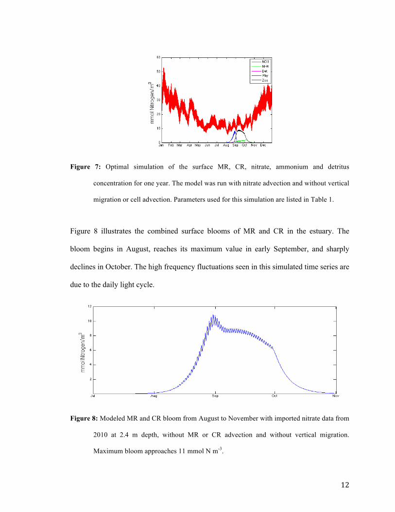
12
Figure 7: Optimal simulation of the surface MR, CR, nitrate, ammonium and detritus
concentration for one year. The model was run with nitrate advection and without vertical
migration or cell advection. Parameters used for this simulation are listed in Table 1.
Figure 8 illustrates the combined surface blooms of MR and CR in the estuary. The
bloom begins in August, reaches its maximum value in early September, and sharply
declines in October. The high frequency fluctuations seen in this simulated time series are
due to the daily light cycle.
Figure 8: Modeled MR and CR bloom from August to November with imported nitrate data from
2010 at 2.4 m depth, without MR or CR advection and without vertical migration.
Maximum bloom approaches 11 mmol N m-3.

13
Chlorophyll (Chl) concentrations as high as 20 µg/l have been observed at the surface of
the Columbia River estuary (Sullivan et al. 2001; CMOP SATURN 03, 2010). Modeled
chlorophyll can be obtained from modeled MR biomass using a Chl:N ratio of 2.1 ± 0.5
mg Chl mmol N-1 (Johnson et al., 2006), This ratio is very similar to what has been
observed for diatoms off the Oregon coast. Dickson (1994) and Dickson and Wheeler
(1995) obtained a Chl:N ratio of 2.19 ± 0.45 mg Chl mmol N-1 from a station 8 km
offshore of Newport from July 1990 to August 1991. Using the 2.1 mg Chl mmol N-1
value for Chl:N, the simulation demonstrates a maximum of 23 mg Chl m-3, which is in
the range of Chl observed at SATURN 03.
Detritus, ammonium, and CR concentrations at the surface have observable responses to
the MR bloom in this simulation. The most obvious relationship is between MR and CR;
once temperature, light, and nutrient conditions in the estuary are favorable,
phytoplankton begin to bloom and MR are able to graze. MR grazing depletes the CR
population faster than the natural mortality rate and exceeds the CR growth rate in
September. Additionally, detritus concentration increases and peaks from mid-August to
early September as MR begins to graze the abundant phytoplankton. “Sloppy feeding” is
one source of detritus; as MR grazes, some of the organic material does not get ingested
and is lost to detritus. The other source of detritus is CR mortality, imposed by the CR
mortality rate parameter. The mortality rates are imposed as a percentage of the total
population. Therefore, as biomass concentration in the bloom increases, mortality also
increases. The MR bloom also triggers increased ammonium concentrations. Ammonium
is the product of excretion and instantaneous remineralization (MR mortality). Its

14
maximum concentration does not exceed 3 mmol N m-3, and its peak coincides with the
beginning of the sharp bloom decline. Concentrations between 1 mmol N m-3 and 3 mmol
N m-3 have been observed in the main channel red water (Herfort et al., 2012).
There does not appear to be a significant depletion of nitrate in response to increasing
MR or CR. In the one-dimensional model, the nitrate lost to nitrogen uptake processes is
negligible compared to the input by advection from the ocean and river. A three-
dimensional model would show the impact of the bloom on nitrate concentration in
greater detail because spatial changes in estuary fluxes are included.
Figure 9: Photosynthetic growth, grazing, and mortality rates (plotted as absolute value for
comparison) of MR at the surface.
In the optimal simulation, there is initially a balance between the three biological forcing
mechanisms, which leads to the MR bloom (photosynthetic growth, grazing, and
mortality). Photosynthetic growth becomes larger than the grazing contribution to MR
growth in early September when grazing begins to decline. By mid-September the rate of

15
growth of the bloom slows down and approaches its peak due to a balance between
photosynthetic growth and mortality of MR. MR has stopped grazing and growth related
to photosynthesis begins to decline as the organs required to photosynthesize deteriorate
without being replaced. At the beginning of October, the mortality rate exceeds the
growth rate and the population makes a sharp decline (controlled by the mortality rate)
that ends in November. Figure 9 illustrates that photosynthesis contributes significantly
more to the MR bloom than grazing, but once grazing has finished the process is unable
to sustain itself and the bloom ends.
3.2 Nitrate Advection
Adding a real flux of nitrate in the model regulates the amount of nitrogen in the system.
Without these fluxes, it would be difficult to reproduce a realistic bloom over multiple
years. Figure 10 shows the optimal model behavior over 3 years, and the impact of
including nitrate advection calculated from observations on the model outputs for the
same 3-year period.
Figure 10a represents an approximation of the biogeochemical response when a
continuous nitrate source from the river takes the form of a hyperbolic tangent function
(Figure 10b). The curve imposes 20% maximum inlet river flows carrying nitrate in the
winter, has a steep increase of 10% per month from March to May, a steep decrease of
10% from August to October, and peak in the middle of June. A constant nitrate
concentration input is applied to these flows, providing about 40 mmol N m-3 from

16
(a) (b)
(c) (d)
Figure 10: (a) A three-year run with approximated nitrate source based on (b) a hyperbolic
tangent function controlling the percent maximum nitrate source from the river over the
year. (c) A three-year run of the basic case without nitrate advection. (d) Optimal
simulation: a three-year run with nitrate advection. Note that the scales differ between
different model runs.
January to June. The function is based upon Columbia river flow trends (U.S. Bureau of
Reclamation, U.S. Army Corp of Engineers, and Bonneville Power Administration,
2001); however, it does not account for water entering/exiting the ocean, nor is it a

17
substitute for measured data, especially since a reasonable constant nitrate concentration
range that can be applied to this approximation is uncertain. Figure 5 illustrates the
dynamic seasonal change in nitrate concentration measured from the river and ocean over
the course of one year.
In Figure 10d, the nitrate concentrations from Figure 5 are applied to an advection term to
simulate realistic fluctuations in nitrate concentration in the estuary. Annual nitrate
advection patterns lead to a realistic bloom of MR and CR in the late summer and fall
(Figure 10d) while MR and CR are unable to bloom multiple years without an external
source of nutrients (Figure 10c). With nitrate advection in the optimal simulation (Figure
10d), the imposed nitrate concentration exceeds the model requirements to sustain a
bloom, which leads to model results that are comparable to observed trends in the
Columbia River estuary. The model is also more stable in the presence of slight
parameter deviations from Table 1 values due to the abundance of nitrate.
3.3 Maximum Uptake Rate
Based on the literature surveyed during this study, it appears that there is a large
uncertainty on the maximum nutrient uptake rate of MR, and the question of whether MR
and CR have the same maximum nutrient uptake rate is still open (Peterson et al., 2012 &
2013). Nutrient uptake is a necessary component to MR and CR growth during
photosynthesis. Equations 1 and 2 include NO3 and NH4 uptake in the calculation of
photosynthetic growth for MR and CR, and the uptake terms are calculated with the

18
Michaelis-Menten formulation (see Equation 10 in Appendix A). The model was
designed to accommodate unequal maximum uptake rates in MR and CR so that
scenarios with equal and unequal uptake rates could be tested. A sensitivity analysis is
explored in Figure 11.
(a)
(b)
Figure 11: (Left) Surface concentrations over one year and (right) MR photosynthesis, grazing
and mortality for the following simulations: (a) VM = ZM = 1.00 d-1, and (b) VM = ZM =
1.37 d-1.

19
(c)
Figure 11 (continued): (Left) Surface concentrations over one year and (right) MR
photosynthesis, grazing and mortality for the following simulations: (c) VM = 1.37 and
ZM = 1.00 d-1. VM is the CR uptake rate and ZM is the MR uptake rate. Note that the scales
vary between the different model runs and between the left and right plots within each
model run. In the optimal simulation, VM = 1.00 d-1 and ZM = 1.37 d-1.
The model is highly sensitive to a change in CR maximum uptake rate. A 0.37 d-1
increase in the CR (Figures 11b-c) maximum uptake rate results in CR blooms occurring
two months earlier, with a maximum nearly three times the value from the optimal
simulation (Figure 7). The MR bloom lasts twice as long and achieves a maximum that is
approximately 10 times higher than in the optimal simulation in Figure 11b. When the
MR uptake rate is concurrently decreased by the same amount, the MR bloom reaches
about twice its optimal simulation maximum. In both cases, the beginning of the MR
bloom still occurs half a month after the beginning of the CR bloom and length of the CR
bloom is reduced by a few days compared to the optimal run. A 0.37 d-1 decrease of MR
uptake rate while keeping the CR uptake rate from the optimal simulation does not show
large changes in either timing or magnitude of the CR and MR bloom (Figure 11 a).
20
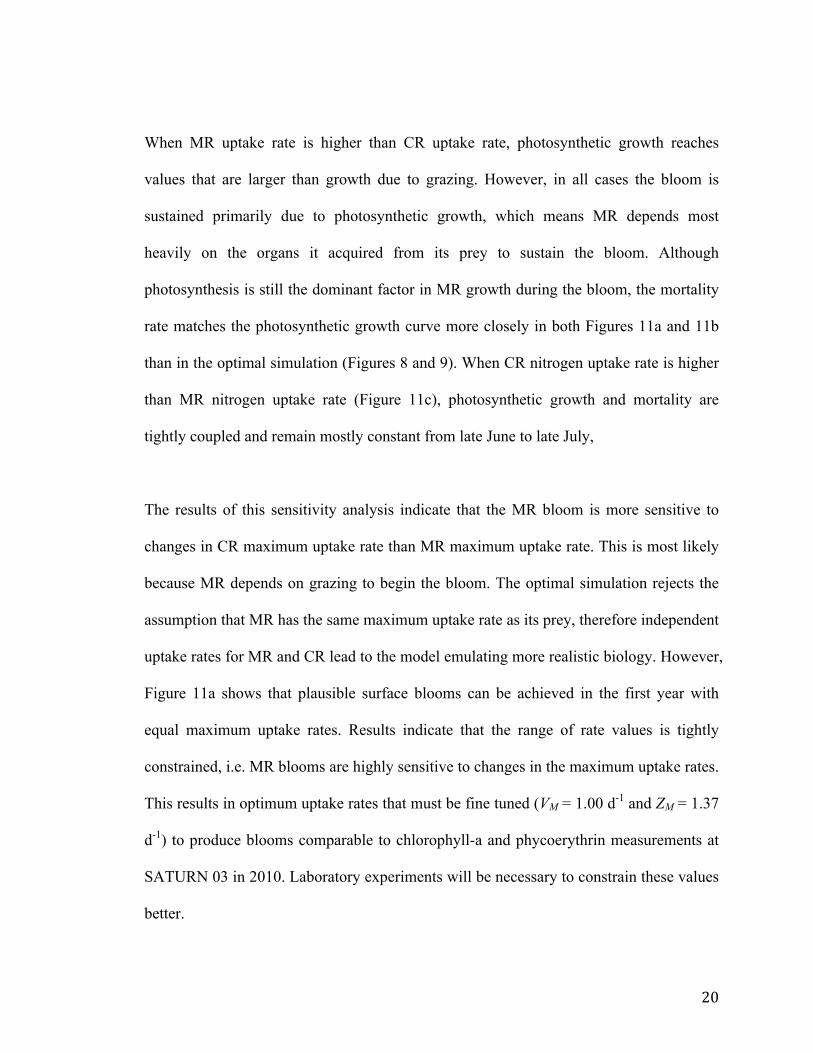
When MR uptake rate is higher than CR uptake rate, photosynthetic growth reaches
values that are larger than growth due to grazing. However, in all cases the bloom is
sustained primarily due to photosynthetic growth, which means MR depends most
heavily on the organs it acquired from its prey to sustain the bloom. Although
photosynthesis is still the dominant factor in MR growth during the bloom, the mortality
rate matches the photosynthetic growth curve more closely in both Figures 11a and 11b
than in the optimal simulation (Figures 8 and 9). When CR nitrogen uptake rate is higher
than MR nitrogen uptake rate (Figure 11c), photosynthetic growth and mortality are
tightly coupled and remain mostly constant from late June to late July,
The results of this sensitivity analysis indicate that the MR bloom is more sensitive to
changes in CR maximum uptake rate than MR maximum uptake rate. This is most likely
because MR depends on grazing to begin the bloom. The optimal simulation rejects the
assumption that MR has the same maximum uptake rate as its prey, therefore independent
uptake rates for MR and CR lead to the model emulating more realistic biology. However,
Figure 11a shows that plausible surface blooms can be achieved in the first year with
equal maximum uptake rates. Results indicate that the range of rate values is tightly
constrained, i.e. MR blooms are highly sensitive to changes in the maximum uptake rates.
This results in optimum uptake rates that must be fine tuned (VM = 1.00 d-1 and ZM = 1.37
d-1) to produce blooms comparable to chlorophyll-a and phycoerythrin measurements at
SATURN 03 in 2010. Laboratory experiments will be necessary to constrain these values
better.

21
3.4 Mortality Rate
The mortality rate of MR has a direct impact on the slope of population decline at the end
of an MR bloom. CR mortality rate indirectly affects the timing and magnitude of the MR
bloom through grazing. These parameters are imposed as a percent mortality of the entire
population (refer to Equations 1 and 2) of their respective species. Figure 12 explores
simulation sensitivity to changes in planktonic mortality rates.
(a)
(b)
(c)
Figure 12: Surface level concentrations with
best case parameters and changing mortality
rates over one year. Mortality rates (d-1) are (a)
mp = mz = 0.33, (b) mp = mz = 0.145, and (c)
mp = 0.145, mz = 0.33. The optimal simulation
parameter values are mp = 0.33 and mz = 0.145.
These fractions may be translated to percentages
of the population.

22
The elevated CR mortality rate in Figure 12a and the optimal simulation causes the MR
to bloom once a year in September. When the CR mortality rate is reduced from 33%
mortality to 14.5%, MR initially bloom in the month of June, with the potential to bloom
once or twice more in the same year given prey and nutrients are abundant. Figures 12b
and 12c demonstrate a 66% decrease in the first bloom’s maximum concentration when
the CR mortality rate remains at 14.5% and the MR mortality rate increases from 14.5%
to 33%. A similar difference (approximately 50%) in the initial bloom peak
concentrations occurs when the MR mortality rate increases compared to the optimal
simulation (Figures 7 and 12a).
The frequency of MR blooms in a year depends on both MR and CR mortality rates,
because timing is strongly influenced by prey concentration. This makes it difficult to
compare second and third blooms in a year between different runs. The MR mortality rate
has a direct impact on the magnitude of the bloom; however, because MR depend on
grazing to start a bloom, the mortality rate of MR does not directly correlate with the
timing or frequency of blooms in a given year. Timing of the first bloom can instead be
inversely correlated with the CR mortality rate. A higher CR mortality rate will delay
both the CR and MR blooms by removing CR cells rapidly, reducing the remaining
number of reproductive cells, and reducing the MR cell initial source of growth. An
elevated MR mortality rate will reduce the total MR population, but it will not impact the
rates of grazing and photosynthesis per unit MR. Once mortality begins to outcompete
grazing and photosynthesis, the population declines at a rate that is proportional to the
mortality. Higher MR mortality rates allow more CR to grow since the total number of

23
grazed prey cells is reduced. This, in conjunction with a reduced CR mortality rate, can
trigger one or two additional CR and MR blooms in one year.
3.5 Rate of Photosynthesis
Plots of photosynthesis, grazing and mortality rates for MR illustrate the role each plays
in the shape of an MR bloom. Grazing instigates the bloom, determines when the bloom
starts and facilitates a rapid climb in MR concentration. The bloom maximum often
occurs at the end of the grazing period or shortly after photosynthesis becomes the
driving force for growth. Photosynthesis sustains the bloom. Then the mortality rate
controls the peak of the bloom and shapes the decline. Mortality in conjunction with
photosynthesis determines when the end of the bloom occurs. Grazing and mortality rate
have been discussed at length in earlier parts of this analysis. This section will explore the
sensitivity of MR bloom characteristics to photosynthesis, specifically by manipulating
the maximum CR to MR cell ratios involved in MR photosynthesis.
As mentioned in section 2, photopop is a function that imitates the limitation of growth
based on the number of CR grazed with symbiont deterioration over a 30 day period.
From the moment they are absorbed, symbionts deliver diminishing returns over time,
with total degradation (no effect on growth) of the given symbiont after day 30 (refer to
Equation 7). An additional limitation is imposed by Equation 8 to control the maximum
amount of CR that may be absorbed by MR at a given point in time. If the number of CR
per MR cell is greater than a given value maxthMR, then MR does not acquire more CR

24
for photosynthesis but still continues to graze. This is mathematically imposed in the
model when the lower maxthMR value replaces the higher photopop value that is
calculated from grazing.
𝑚𝑎𝑥𝑡ℎ𝑀𝑅 = 𝑎 𝑟 𝐶𝑅,𝑀𝑅 (8)
where a is the ratio of nitrogen content in CR and MR cells and r(CR,MR) represents the
number of CR cell per MR cell.
Since our model is in terms of nitrogen and the nitrogen content of CR and MR cells are
largely different, it is imperative to take into account this difference. For this study we
considered 669 pg C cell-1 and a C:N ratio of 5 mmol C:mmol N for Mesodinium and 29
pg C cell-1 and a C:N of 5 mmol C:mmol N for cryptophyte (Johnson and Stoeker, 2005;
Johnson et al., 2006). The value of r(CR,MR) is set to 10 in the optimal simulation based
on literature review (Yih et al., 2004). Both photopop and its upper limit maxthMR play a
significant role in MR photosynthesis rate, the first term in the zooplankton component
calculation (Equation 2).
The sensitivity analysis in Figure 13 focuses specifically on the relationship between the
variable r(CR,MR) in the maxthMR calculation and the dynamics of the MR bloom. A
change of r(CR,MR) from 1 to 10 triggers an earlier bloom by a few days and a slight
increase in the MR bloom maximum. It is interesting to note that a single CR cell is
capable of triggering a MR bloom that is comparable to the result of 10 CR cells, given

25
sufficient nutrients. This supports the notion that MR is capable of sustaining a bloom
even after grazing only a single CR cell. The change of r(CR,MR) from 10 to 20 is far
more significant. The peak of the MR bloom appears to respond non-linearly to an
elevated absorption limit, but there is a clear correlation between the absorption limit and
the peak of the MR bloom because absorption facilitates photosynthetic growth. A less
drastic change in the timing and length of MR bloom occurs in response to a change from
1 to 20 in the CR absorption maximum. However, as r(CR,MR) increases, the bloom
starts earlier in the year, peaks earlier, and lasts longer. The change of r(CR,MR) from 1
to 20 doubles the length of the MR bloom from less than one month in September to
approximately two months from mid-August to mid-October.
There is also a marked decrease in CR population as the absorption limit increases
(primarily compared between Figures 13b and 13a). The beginning of the CR bloom is
unaffected by any change in absorption limit, so it begins in August in every run of this
sensitivity analysis. However, as r(CR,MR) increases, the CR peak occurs sooner,
achieves a lower concentration, and declines sooner because there are more grazers.
If the limit of CR absorption by MR is increased, MR is able to absorb more symbionts
through grazing and therefore grow more MR through photosynthesis. The elevated MR
then translates to a larger population that can graze CR. More CR are grazed, then
absorbed, and converted to MR growth. This cycle perpetuates until the CR population is
lost to grazing.

26
(a)
(b)
(c) Figure 13: (Left) Surface concentrations over one year with optimal simulation parameters and
(right) MR photosynthesis, grazing and mortality with the maximum CR:MR cell ratios
for MR photosynthesis: (a) 1, (b) 10 (optimal simulation), and (c) 20. Note the different
scales between the figures.
27
The model currently includes perpetual MR grazing, independent of absorption limits and
photosynthesis. It is known that in species like Karlodinium, photosynthesis is
supplemented with feeding on cryptophytes (Adolf et al., 2006); however it is unknown
whether MR mirrors this behavior. Further sensitivity analysis should be conducted with
the grazing turned off during photosynthesis to isolate the effects of each process on the
MR bloom. As an initial prediction, one may expect to see a small or negligible decrease
in the peak of the MR bloom, but a longer bloom time (with the same start date) or
increased propensity for multiple blooms due to higher concentrations of available prey
when the MR cells are not photosynthesizing. Photosynthesis drives the growth rate to its
peak while grazing extends the length of the bloom.
3.6 Seed Concentrations
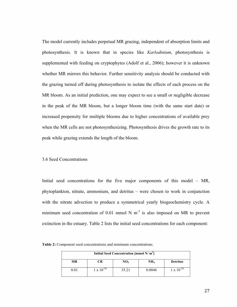
Initial seed concentrations for the five major components of this model – MR,
phytoplankton, nitrate, ammonium, and detritus – were chosen to work in conjunction
with the nitrate advection to produce a symmetrical yearly biogeochemistry cycle. A
minimum seed concentration of 0.01 mmol N m-3 is also imposed on MR to prevent
extinction in the estuary. Table 2 lists the initial seed concentrations for each component:
Table 2: Component seed concentrations and minimum concentrations.
Initial Seed Concentration [mmol N/ m3]
MR CR NO3 NH4 Detritus
0.01 1 x 10⁻¹⁰ 35.21 0.0046 1 x 10⁻¹⁰

28
Over several years, the initial seed concentration has a noticeable impact on bloom
patterns and MR minimum concentration has a significant impact on the initialization of
a bloom. The model sensitivity is most visible below the estuary surface. An analysis on
the impact of initial concentrations over three years is explored in Figure 14.
(a) (b)
(c) (d)
Figure 14: Nutrient and biological concentrations through the water column over time. The five
components are as follows: (a) MR, (b) CR, (c) nitrate, (d) ammonium,

29
(e)
Figure 14 (continued): (e) detritus.
The surface level concentrations appear to be symmetrical in timing and magnitude every
year over a three-year period (Figures 10c and 14). This result validates the inclusion of
nitrate advection in the model; however, with the current initial conditions and imposed
minimum concentrations, Figure 14 demonstrates that the yearly pattern does not hold
constant through the water column.
Annual bloom similarity is most strongly affected by the seed concentrations. The initial
concentrations listed in Table 2 were sufficient to produce nearly identical bloom patterns
at the surface with the addition of nitrate advection. However, optimization to produce
identical yearly blooms throughout the water column is ongoing. A run simulating
several years will approach an asymptote of similarity, beginning with very disparate
concentrations between initial years and producing increasing similar concentration
patters between later years. The results of a 5-year run with seed concentrations listed in
30
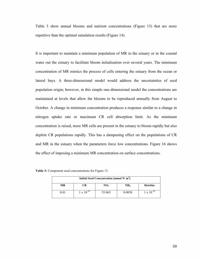
Table 3 show annual blooms and nutrient concentrations (Figure 15) that are more
repetitive than the optimal simulation results (Figure 14).
It is important to maintain a minimum population of MR in the estuary or in the coastal
water out the estuary to facilitate bloom initialization over several years. The minimum
concentration of MR mimics the process of cells entering the estuary from the ocean or
lateral bays. A three-dimensional model would address the uncertainties of seed
population origin; however, in this simple one-dimensional model the concentrations are
maintained at levels that allow the blooms to be reproduced annually from August to
October. A change in minimum concentration produces a response similar to a change in
nitrogen uptake rate or maximum CR cell absorption limit. As the minimum
concentration is raised, more MR cells are present in the estuary to bloom rapidly but also
deplete CR populations rapidly. This has a dampening effect on the populations of CR
and MR in the estuary when the parameters force low concentrations. Figure 16 shows
the effect of imposing a minimum MR concentration on surface concentrations.
Table 3: Component seed concentrations for Figure 15.
Initial Seed Concentration [mmol N/ m3]
MR CR NO3 NH4 Detritus
0.01 1 x 10⁻¹⁰ 35.065 0.0058 1 x 10⁻¹⁰

31
(a) MR (b) CR
(c) NO3 (d) NH4
(e) Detritus
Figure 15: Nutrient and biological concentrations that produce similar yearly patterns through the
water column from seed concentrations listed in Table 3 and parameters listed in Table 1.

32
(a) (b)
Figure 16: (a) Surface concentrations over two years with the initial seed concentrations in Table
3 and without minimum concentrations. (b) Surface concentrations over two years with
the same seed concentrations and a minimum concentration of 0.01 mmol N m-3 for MR.
3.7 Vertical Migration
MR possess an essential survival skill: the ability to swim up to 1.2 cm s−1 (Hansen and
Fenchel, 2006). This means that MR do not behave like passive particles in the dynamic
estuary environment. The ciliates are capable of swimming away from the surface when
a strong flux threatens to flush them out of the estuary, then return to the surface to
continue photosynthesis and grazing. The current model contains an adjustable
swimming speed (swimmax). The speed is the amplitude of the periodic swimming
velocity calculated from Equation 6, a simplified equation derived from the tidal
frequency and phase. Figure 17 illustrates the sensitivity analysis of CR/MR biomass and
nutrient concentrations at the surface and MR biomass at depth in the presence of a
changing maximum swim speed (swimmax).

33
(a)
(b)
(c)
Figure 17: (Left) Surface level concentrations over one year with optimal simulation parameters
and (right) MR concentrations throughout the column over time. The parameter swimmax
had the following values each run: (a) swimmax = 0.035 mm/s, (b) swimmax = 0.135, (c)
swimmax = 0.235,
34
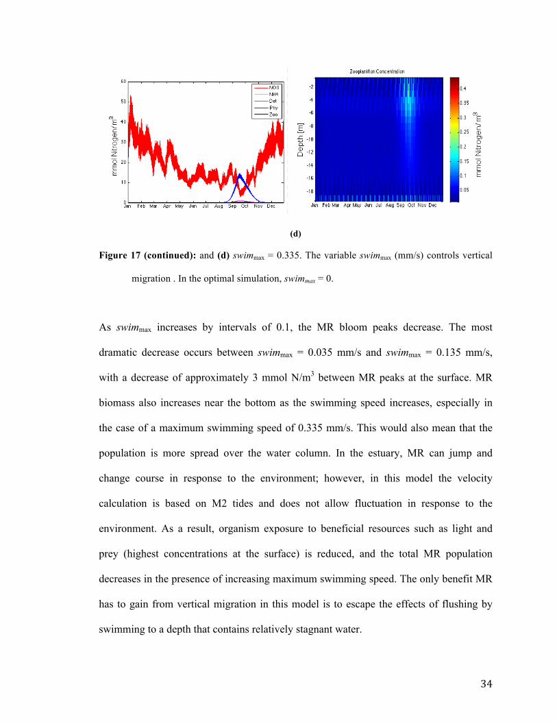
(d)
Figure 17 (continued): and (d) swimmax = 0.335. The variable swimmax (mm/s) controls vertical
migration . In the optimal simulation, swimmax = 0.
As swimmax increases by intervals of 0.1, the MR bloom peaks decrease. The most
dramatic decrease occurs between swimmax = 0.035 mm/s and swimmax = 0.135 mm/s,
with a decrease of approximately 3 mmol N/m3 between MR peaks at the surface. MR
biomass also increases near the bottom as the swimming speed increases, especially in
the case of a maximum swimming speed of 0.335 mm/s. This would also mean that the
population is more spread over the water column. In the estuary, MR can jump and
change course in response to the environment; however, in this model the velocity
calculation is based on M2 tides and does not allow fluctuation in response to the
environment. As a result, organism exposure to beneficial resources such as light and
prey (highest concentrations at the surface) is reduced, and the total MR population
decreases in the presence of increasing maximum swimming speed. The only benefit MR
has to gain from vertical migration in this model is to escape the effects of flushing by
swimming to a depth that contains relatively stagnant water.

35
This simple, one dimensional model could not retain MR in the presence of advection
when MR and CR advection were calculated similarly to nitrate advection (Equation 15,
Appendix A) and fluxes were uniform over the vertical. MR was unable to sustain any
bloom in the presence of advection due to flushing; however, a CR bloom could be
observed at the surface because CR growth was able to outcompete the effects of
advection by relatively high growth rates. The simulation was then modified to advect
only the top half of the estuary column while the bottom half remained stationary with
supplementary MR cell concentrations from the ocean. If it had the correct vertical
migration pattern, theoretically MR would be able to swim to the stagnant level of water
while high river fluxes drove advection at the surface, after which the cells could return
to the surface to photosynthesize. Unfortunately, MR could not escape the effects of
flushing in this scenario either.
Two obstacles prevent the simulation from effectively modeling an MR bloom in the
presence of advection with the aid of vertical migration. First, the current optimal
simulation parameters restrict the maximum swimming speed of MR. If MR swims too
quickly, it spends so little time at the surface of the estuary that it is unable to
photosynthesize. This reduces the overall population of MR in the water column. Second,
the current advection model is such that MR cannot escape flushing by swimming to a
different depth as the advection is uniform on the vertical. In order to test the swimming
part of the model, a more sophisticated advection profile would be required so that a
different flux could be imposed at each depth in a given time. Additionally, the

36
simulation could be expanded to a three-dimensional model that provides lateral bays to
aid MR, CR, and nutrient retention, as lateral bays experience lower velocities and
transport than the channels.
4. Conclusion
Sensitivity analysis of the optimal one-dimensional NNPZD model illustrates a dynamic
relationship between MR, its prey CR, and effects on the biogeochemistry of the estuary
over multiple years. Most of the parameters are positively correlated with the MR and CR
bloom timing, duration, and peak. This includes maximum uptake rates, photosynthesis
rates, seed concentrations, and MR vertical migration. Due to the MR photoautotrophy
dependence on their prey, parameters related to CR have the strongest impact on the MR
bloom. An optimal simulation setup was successfully parameterized with respect to
nitrate advection, MR and CR maximum uptake rates, MR and CR mortality rates, MR
photosynthesis rate, and minimum concentrations. Vertical migration and the advection
of MR and CR were also explored. However, many uncertainties remain in constraining
parameters, some of which significantly influence the MR bloom. The areas detailed
below should be explored further in future MR modeling studies.
The sensitivity of the MR bloom to grazing through photosynthesis (the current model) in
comparison to photosynthesis without grazing should be tested. The result could buoy CR
populations, which may extend MR blooms or trigger MR blooms earlier in the
subsequent cycle. It is expected that the difference in maximum MR population during a

37
cycle would be negligible. Photosynthesis is the primary contributor to MR growth and
the driving force for high MR concentrations.
Maximum uptake rates were tested, but the P-I curve might also be important. The
expectation is that changes in the P-I curve will produce the same results as changes in
the uptake rates. The P-I curve is directly involved in the light limitation calculation
(Equation 12 in Appendix A), which in turn is used to calculate MR and CR
photosynthetic growth. If the P-I curve has a similar relationship to photosynthetic
growth as nutrient uptake, the simulation may be equally sensitive to changes in the
initial slope of the P-I curve as it is to the uptake rates. Little is known with respect to the
photosynthesis rate of MR in the Columbia River estuary compared to other strains such
as the Antarctic species (Johnson et al., 2006). Therefore testing the sensitivity of MR to
parameters that are known to affect photosynthesis may yield some insights into the
organism and its relationship with the estuary.
Future work should also allow the fluxes from the ocean and river to the estuary to be
vertically variable so the water column can mimic the depth-dependent effect of the tides
(flood and ebb). This would present a more realistic representation of advection, and
provide a means to test MR retention time due to vertical migration in the presence of
advection. A sensitivity analysis of the swimming speed, migration cycle between the
surface and bottom of the water column, and fluxes with and without MR concentration
in the ocean should be conducted and compared to observed data in the Columbia River
estuary. The use of a two-dimensional channel representing the main channel of the

38
estuary might be a first approach to test the vertical migration speed with short enough
simulations to perform sensitivity analyses.
Finally, it is recommended that oxygen be added to the model to assess the impact of MR
on the oxygen cycle in the estuary. This is of special interest to local fishing businesses
and environmental groups because of the sensitivity of some species, such as salmon, to
oxygen concentration in the water. At this time, it is known that oxygen concentration
changes in response to both consumption and production by MR and CR. Preliminary
simulation runs with oxygen were calculated using Equation 9 (Appendix A). This
equation subtracts respiration of CR and MR from the production of oxygen in the
estuary with an air-sea interaction component. The calculation depends on the same
parameters as the rest of the model, which means that oxygen is controlled by the same
processes that have been addressed in the sensitivity analysis. The results of preliminary
oxygen simulation experiments illustrate an increase of oxygen concentration from
baseline values between August and October in the Columbia River estuary due to MR
and CR photosynthesis during blooms. This trend has been observed in the Columbia
River estuary, and further testing may clarify the relationship between oxygen and other
elements of the NNPZD network.

39
References
Adolf et al. (2006) The balance of autotrophy and heterotrophy during mixotrophic growth of Karlodinium micrum (Dinophyceae), Journal of Plankton Research, 28: 737-751. Barth, J. A. and Wheeler, P.A. (2005) Introduction to special section: Coastal Advances in Shelf Transport. Journal of Geophysical. Research. 110(C10), C10S01, doi:10.1029/2005JC003124. Cloern, J. E. (1991) Tidal stirring and phytoplankton bloom dynamics in an estuary. Journal of Marine Research 49: 203–221. Crawford et al. (1997) Recurrent Red-tides in the Southampton Water Estuary Caused by the Phototrophic Ciliate Mesodinium rubrum. Estuarine, Coastal and Shelf Science, 45: 799–812. Garcia-Cuetos et al. (2012) Studies on the genus Mesodinium II. Ultrastructural and molecular investigations of five marine species help clarifying the taxonomy. Journal of Eukaryote Microbiology, 59: 374-400. Hansen et al. (2013) Acquired phototrophy in Mesodinium and Dinophysis – A review of cellular organization, prey selectivity, nutrient uptake and bioenergetics. Harmful Algae, http://dx.doi.org/10.1016/j.hal.2013.06.004 Hansen, P. J. and Fenchel, T. (2006) The bloom-forming ciliate Mesodinium rubrum harbours a single permanent endosymbiont. Marine Biology Research, 2: 169-177. Herfort et al. (2011) Myrionecta rubra population genetic diversity and its cryptophyte chloroplast specificity in recurrent red tides in the Columbia River estuary. Aquatic Microbial Ecology. 62 Herfort et al. (2012) Red waters of Myrionecta rubra are biogeochemical hotspots for the Columbia River estuary with impacts on primary/secondary productions and nutrient cycles. Estuaries and Coasts, 35: 878-891, DOI 10.1007/s12237-012-9485-z Ivlev, V. S. (1961) Experimental ecology of the feeding of fishes. Yale University Press, New Haven, Connecticut, USA. Johnson, M.D. and Stoeker D.K (2005) Role of feeding in growth and phytophysiology of Myrionecta rubra. Aquatic Microbial Ecology, 39:303-312. Johnson et al. (2006) Sequestration, performance, and functional control of cryptophyte plastids in the ciliate Myrionecta rubra (ciliophora). Journal of Phycology, 42: 1235–1246.

40
Johnson et al. (2007) Retention of transcriptionally active cryptophyte nuclei by the ciliate Myrionecta rubra. Nature, 445: 426-428. Kim et al. (2008) Growth and grazing responses of the mixotrophic dinoflagellate Diophysis acuminata as functions of light intensity and prey concentration. Aquatic Microbial Ecology, 51: 301-310. Lindholm T. (1985), Mesodinium rubrum – a unique photosynthetic ciliate. Advances in Aquatic Microbiology, 3: 1-48. Michaelis, L. and Menten, M.L. (1913). Die Kinetik der Invertinwirkung. Biochem Z, 49: 333–369 Peterson et al. (2013) Associations between Mesodinium rubrum and cryptophyte algae in the Columbia River estuary. Aquatic Microbial Ecology. 68(2) Peterson et al. (2012) Red waters of Myrionecta rubra are biogeochemical hotspots for the Columbia River estuary with impacts on primary/secondary productions and nutrient cycles. Springer Link, 35: 878-891. Spitz, Y. H. et al. (2005) Modeling of ecosystem processes on the Oregon shelf during the 2001 summer upwelling, J. Geophys. Res., 110, C10S17, doi:10.1029/2005JC002870. Spitz, Y.H. (2011) Ecosystem Modeling of the Oregon Shelf: Everything but the Kitchen Sink. Interdisciplinary Studies on Environmental Chemistry—Marine Environmental Modeling & Analysis, Eds., K. Omori, X. Guo, N. Yoshie, N. Fujii, I. C. Handoh, A. Isobe and S. Tanabe, pp. 1–9 Spitz, Y.H. et al. (2015) Study of the Formation, Retention and Ecological Impact of a Mesodinium Bloom in the Columbia River Estuary – A model approach, In preparation. U.S. Bureau of Reclamation, U.S. Army Corp of Engineers, and Bonneville Power Administration. (2001) The Columbia River System: The Inside Story. 2: 1-80 Wilkerson, F. P. and Gruneisch G. (1990) Formation of blooms by the symbiotic ciliate Mesodinium rubrum: the significance of nitrogen uptake. Journal of Plankton Research, 12: 973-989. Yih et al. (2004) Ingestion of cryptophyte cells by the marine photosynthetic ciliate Mesodinium rubrum. Aquat. Microb. Ecol., 36: 165-170. Zhang, Y. and Baptista, A. M. (2008) SELFE: A semi-implicit Eulerian–Lagrangian finite-element model for cross-scale ocean circulation. Ocean Modeling. 21(3-4): 71-96. Appendices

41
A. Functions used in the model equations
• Nitrate and ammonium uptake was calculated using the classical Michaelis-Menten
formulation (Michaelis and Menten, 1913).
€
uptakeN =VM × NKs + N
(A1)
where VM is the maximum uptake rate and Ks is the concentration at ½ VM.
• Ivlev grazing was used to describe the consumption of phytoplankton (CR) by
zooplankton (MR) (Ivlev, 1961).
€
graz = rM × [1− e−λP ] (A2)
where rM is the maximum grazing rate, and λ is the Ivlev constant. P is the
phytoplankton concentration.
• The light limitation function is defined as
lightlim =α I
VM2 +α 2I 2
(A3)
where
is the solar radiation, α is the initial slope of the P-I curve, and VM is the maximum uptake
rate. kw, kp and kz are the coefficient of light attenuation by seawater, cryptophyte and
Mesodinium rubrum. I0 is the surface radiation obtained from the 2001 solar radiation

42
measurements at a mooring off Newport, Oregon, during the Coastal Ocean Advances in
Shelf Transport (COAST) program (Barth and Wheeler, 2005). This includes the daylight
cycle.
• The temperature limitation was defined to represent the seasonal variability of the
temperature in the Columbia River estuary and favor growth during the warm period
of summer-early fall (Figure 18).
templim = 0.75+ 0.1× tanh 0.00055× 1− 224dt
#
$%&
'(+44dt
)
*+
,
-.
#
$%
&
'( (A4)
+ 0.1× tanh −0.00055× 1− 224dt
#
$%&
'(−44dt
)
*+
,
-.
#
$%
&
'(
where the tanh function produces the curve in Figure A1.
Figure A1: Function to limit MR and CR growth during cold seasons.
• The advection of nitrate is defined from the fluxes and concentrations from the river
and ocean sides into the domain and from the modeled nitrate to the ocean and river.

43
€
AdvecNO3 = FlowRiverIn *ConcRiver + FlowRiverOut *NO3 (A5)− FlowOceanIn *ConcOcean − FlowOceanOut *NO3
where FlowRiverIn is the flux of water from the river source into the estuary,
FlowRiverOut is the flux of water from the estuary into the river, FlowOceanIn is the
flux of water from the ocean source into the estuary, FlowOceanOut is the flux of
water from the estuary into the ocean, ConcRiver is the concentration of NO3 in the
river source, and ConcOcean is the concentration of NO3 in the ocean source.
• Oxygen changes over time due to the biological sink (respiration) and source
(production) and air-sea fluxes. The biological sources and sinks only are represented
here.
∂O∂t
= rO2NO3 × (uptakeNO3 + lightlim× templim×CR+uptakeNO3 × lightlim (A6)
× templim× photopop×MR)− 2×Ω×NH4 + rO2NH4 × (uptakeNH4
+ lightlim× templim×CR+uptakeNH4 × lightlim× templim× photopop×MR−mz×MR− rem×D)
where rO2NO3 is the stoichiometric ratio of O2:NO3 and rO2NH4 is the stoichiometric
ratio of O2:NH4.
44
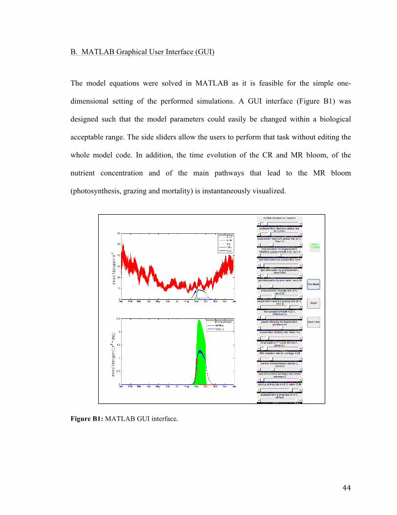
B. MATLAB Graphical User Interface (GUI)
The model equations were solved in MATLAB as it is feasible for the simple one-
dimensional setting of the performed simulations. A GUI interface (Figure B1) was
designed such that the model parameters could easily be changed within a biological
acceptable range. The side sliders allow the users to perform that task without editing the
whole model code. In addition, the time evolution of the CR and MR bloom, of the
nutrient concentration and of the main pathways that lead to the MR bloom
(photosynthesis, grazing and mortality) is instantaneously visualized.
Figure B1: MATLAB GUI interface.