a model of gender inequality and ecomoic growth · this paper introduces a model of gender...

ASIAN DEVELOPMENT BANK

AsiAn Development BAnk6 ADB Avenue, Mandaluyong City1550 Metro Manila, Philippineswww.adb.org

A Model of Gender Inequality and Economic Growth

This paper introduces a model of gender inequality and economic growth. The model is calibrated using microlevel data of Asian economies, and numerous policy experiments are conducted to investigate how various aspects of gender inequality are related to the growth performance of the economy. The analysis shows that improving gender equality can contribute significantly to economic growth by changing females’ time allocation and promoting their accumulation of human capital.

About the Asian Development Bank

ADB’s vision is an Asia and Pacific region free of poverty. Its mission is to help its developing member countries reduce poverty and improve the quality of life of their people. Despite the region’s many successes, it remains home to the majority of the world’s poor. ADB is committed to reducing poverty through inclusive economic growth, environmentally sustainable growth, and regional integration.

Based in Manila, ADB is owned by 67 members, including 48 from the region. Its main instruments for helping its developing member countries are policy dialogue, loans, equity investments, guarantees, grants, and technical assistance.

adb economicsworking paper series

NO. 475

February 2016

A MODEl Of GENDEr INEquAlIty AND EcONOMIc GrOwthJinyoung Kim, Jong-Wha Lee, and Kwanho Shin

ADB Economics Working Paper Series

A Model of Gender Inequality and Economic Growth Jinyoung Kim, Jong-Wha Lee, and Kwanho Shin

No. 475 | February 2016

Jinyoung Kim ([email protected]) is Professor at Korea University. Jong-Wha Lee ([email protected]) is Professor at the Asiatic Research Institute, Korea University. Kwanho Shin ([email protected]) is Professor at the Department of Economics, Korea University. The study was conducted under the Asian Development Bank's technical assistance on economic analysis for gender and development (RDTA 8620). The authors acknowledge Hanol Lee and Eunbi Song for their research assistance.


Asian Development Bank 6 ADB Avenue, Mandaluyong City 1550 Metro Manila, Philippines www.adb.org

© 2016 by Asian Development Bank February 2016 ISSN 2313-6537 (Print), 2313-6545 (e-ISSN) Publication Stock No. WPS167892-2

The views expressed in this paper are those of the authors and do not necessarily reflect the views and policies of the Asian Development Bank (ADB) or its Board of Governors or the governments they represent.

ADB does not guarantee the accuracy of the data included in this publication and accepts no responsibility for any consequence of their use.

By making any designation of or reference to a particular territory or geographic area, or by using the term “country” in this document, ADB does not intend to make any judgments as to the legal or other status of any territory or area.

Notes: 1. In this publication, “$” refers to US dollars. 2. ADB recognizes “Korea” as the Republic of Korea.

The ADB Economics Working Paper Series is a forum for stimulating discussion and eliciting feedback on ongoing and recently completed research and policy studies undertaken by the Asian Development Bank (ADB) staff, consultants, or resource persons. The series deals with key economic and development problems, particularly those facing the Asia and Pacific region; as well as conceptual, analytical, or methodological issues relating to project/program economic analysis, and statistical data and measurement. The series aims to enhance the knowledge on Asia’s development and policy challenges; strengthen analytical rigor and quality of ADB’s country partnership strategies, and its subregional and country operations; and improve the quality and availability of statistical data and development indicators for monitoring development effectiveness.

The ADB Economics Working Paper Series is a quick-disseminating, informal publication whose titles could subsequently be revised for publication as articles in professional journals or chapters in books. The series is maintained by the Economic Research and Regional Cooperation Department.

CONTENTS TABLES AND FIGURES iv ABSTRACT v I. INTRODUCTION 1 II. THE MODEL 5 A. Model Structure 5 B. Formal Structure of the Model 6 III. CALIBRATION AND BALANCED GROWTH PATH 10 IV. GENDER-BASED POLICIES 12 A. Changes in Steady States 12 B. Transition Dynamics 13 C. Output Costs of Gender Inequality 14 V. CONCLUDING REMARKS 20 APPENDIX 23 REFERENCES 27

TABLES AND FIGURES TABLES 1 Gender Inequality in Education, 2010 2 2 Labor Force Participation Rates, 2010 2 3 Calibrated Parameters 11 4 Steady-State Solutions for the Benchmark Economy 11 5 Impacts of Gender Equality Policies 12 FIGURES 1 Transitional Dynamics between Steady States 15 2 Output Costs of Gender Inequality: Transitional Dynamics With and Without Gender Inequality 19

ABSTRACT This paper introduces a model of gender inequality and economic growth that focuses on the determination of women’s time allocation among market production, home production, child rearing, and child education. The theoretical model is based on Agénor (2012), but differs in several important dimensions. The model is calibrated using microlevel data of Asian economies, and numerous policy experiments are conducted to investigate how various aspects of gender inequality are related to the growth performance of the economy. The analysis shows that improving gender equality can contribute significantly to economic growth by changing females’ time allocation and promoting accumulation of human capital. We find that if gender inequality is completely removed, aggregate income will be about 6.6% and 14.5% higher than the benchmark economy after one and two generations, respectively, while corresponding per capita income will be higher by 30.6% and 71.1% in the hypothetical gender-equality economy. This is because fertility and population decrease as women participate more in the labor market. Keywords: economic growth, gender inequality, human capital accumulation, labor market, overlapping generations model JEL codes: E24, E60, J13, J71

I. INTRODUCTION

The role of women in economic development has been a popular topic in academic and policy debates. The last half century has witnessed a drastic increase in labor participation of women in most developed and developing countries. During this period, the labor participation rate of women has been converging to that of men in most countries, and the gender gap in wages has narrowed down (Duflo 2010). Between 1980 and 2009, the global female labor participation rate increased from 50.2% to 51.8%, while that of male labor participation decreased from 82% to 77.7%, resulting in the decline of the gender differentials from 32% to 26% (World Bank 2012). However, there is still significant underutilization and misallocation of women’s skills and talents. In many developing countries, inequality in access to quality education between girls and boys adversely impacts girls’ ability to build human and social capital, lowering their job opportunities and wage in labor markets. Significant barriers remain to women’s participation in labor markets (Elborgh-Woytek et al. 2013). Supply-side constraints, especially those related to fertility, marriage, and child-rearing, influence the determination of females’ labor market participation. There are also demand-side barriers in society that restrict women’s equitable access to jobs, skills development, and fair earnings.

Although gender disparity in education and labor markets prevails worldwide, it is considered a very important policy issue in Asian economies. Tables 1 and 2 show significant gender gaps in educational opportunities, educational attainment, and labor market participation in selected Asian economies and advanced countries.

The objective of this paper is to develop a model that can analyze the role of gender inequality

on long-term economic growth. We use the model to investigate the determination of female labor market participation, human capital accumulation, and economic growth. We then calibrate the model for a typical Asian economy and conduct simulations to quantitatively measure the opportunity cost of gender inequality in terms of output foregone and the long-term productivity gains and income growth that can be obtained by removing the barriers preventing women from having equal access to education and employment opportunities.

A key source of inequality between women’s and men’s participation in the labor force stems

from the way women allocate their time. At all levels of incomes, women tend to do the majority of housework, and correspondingly, they spend less time on market work. Women in developing countries are likely to be involved more in housework than in market work (Berniell and Sánchez-Páramo 2011, World Bank 2012). Our paper develops a model that can analyze the determination of women’s time allocation causing gender inequality in human capital accumulation and labor market participation, the economic costs of gender inequality, and the impacts of gender equality policies.

Our model builds upon research on endogenous economic growth with human capital as the

engine of growth (Becker, Murphy, and Tamura 1990; Ehrlich and Lui 1991). The studies in this area are based on the models of time allocation (Becker 1985) and the quality–quantity tradeoff in children (Becker and Lewis 1973), and they attempt to account for demographic transitions and persistent economic growth.

Like the authors of these studies, we recognize that individual agents make a rational decision

in allocating their time between labor supply, child-rearing, human capital investment in children, and contributing to household production. We consider human capital investment in children by parents as a source of persistent economic growth. Our model thus investigates the interactions between women’s labor force participation, fertility, and economic growth via human capital accumulation.

2 | ADB Economics Working Paper Series No. 475

Table 1: Gender Inequality in Education, 2010

Country Average Years of Schooling Gross Secondary

Enrollment Ratios Gross Tertiary

Enrollment Ratios Female Male Female Male Female Male

Philippines 8.13 8.72 88.0* 81.3* 31.3* 25.3*Kazakhstan 11.42 11.25 94.7 97.5 46.0 33.0Sri Lanka 10.32 9.98 98.4 96.1 20.3 10.8Singapore 11.22 10.34 - - - -Thailand 8.01 7.88 86.0 81.0 56.2 44.0People’s Republic of China 8.01 7.13 83.5 82.8 24.3 22.4Viet Nam 7.48 6.81 - - 22.4 22.3Bangladesh 6.20 5.69 52.9 47.0 7.8* 13.1*Indonesia 8.10 7.20 78.8 78.1 23.2 26.6India 7.59 4.81 62.4 67.5 15.2 21.0Malaysia 10.66 10.21 65.9 67.9 40.8 33.2Cambodia 5.69 3.96 - - 10.5 17.7Japan 11.69 11.45 101.7 101.5 54.7 61.3Republic of Korea 12.76 11.45 96.6 97.6 85.0 115.0Pakistan 6.24 3.76 29.6 38.3 6.1* 7.2*Reference Finland 11.58 11.64 109.7 104.8 103.6 84.9Sweden 11.43 11.76 97.6 98.6 90.8 59.2Germany 12.68 12.06 99.0 104.0 58.5+ 54.6+United States 13.14 13.23 93.7 92.7 109.1 78.2

- = no data available, * indicates 2009 data, + indicates 2011 data. Sources: Barro and Lee 2013, and UNESCO 2012.

Table 2: Labor Force Participation Rates, 2010

Country Female Male All Female/Male Philippines 50.9 80.9 65.9 0.63 Kazakhstan 74.0 81.0 77.4 0.91 Sri Lanka 38.0 81.1 59.3 0.47 Singapore 62.9 82.5 72.8 0.76 Thailand 69.8 84.7 77.1 0.82 People’s Republic of China 75.2 85.3 80.4 0.88 Viet Nam 78.1 84.5 81.2 0.92 Bangladesh 59.8 86.8 73.4 0.69 Indonesia 53.2 86.3 69.7 0.62 India 30.3 83.1 57.7 0.36 Malaysia 46.3 78.9 62.8 0.59 Cambodia 81.8 87.5 84.5 0.93 Japan 63.2 84.8 74.0 0.75 Republic of Korea 54.5 77.1 65.8 0.71 Pakistan 23.0 85.9 54.9 0.27 Reference Finland 72.5 76.7 74.6 0.95 Sweden 76.7 82.2 79.5 0.93 Germany 70.8 82.4 76.6 0.86 United States 68.4 79.6 73.9 0.86

Source: OECD 2012.

A Model of Gender Inequality and Economic Growth | 3

Cross-country and time-series evidence suggests that there is a U-shaped relationship between per capita gross domestic product (GDP) and female labor market participation (Elborgh-Woytek et al. 2013). Boserup (1970) argues that men’s privileged access to education excludes women from the labor force during the early stage of development, and it is only later that women gain access to education and employment. On the other hand, Goldin (1990) interprets the U-shaped pattern as a strong income effect at the early stage and a dominant substitution effect at the later stage.

Despite the general predictions of the positive effect of economic development on female labor market participation, it is not very clear that income increase alone can bring about gender equality in labor market participation. A survey by Cuberes and Teignier (2012) summarizes the three main channels through which increases in income reduce the gender gap in labor market participation, as follows: (i) the income elasticity channel (Becker and Lewis 1973), (ii) technological progress (Greenwood, Seshadri, and Yorukoglu 2005), and (iii) changes in women’s property rights (Doepke and Tertilt 2009). Other papers, like Fernandez (2009) and Dollar and Gatti (1999), highlight the importance of cultural and religious characteristics as determinants of female labor force participation. Steinberg and Nakane (2012) find that differences in public policies significantly explain the differences in female labor participation rates across countries. Our model considers cultural and social factors, including gender bias in child-rearing and education, bargaining power in home production, and labor market discrimination, as important determinants of females’ time allocation and labor market participation.

There is a vast amount of literature on gender equality and growth. The existing theoretical

literature emphasizes that gender equality influences growth via three channels: female labor market participation, average human capital stock, and fertility.

The effects of gender gaps in education on economic growth arise primarily from the impact of

female education on fertility and on the creation of human capital for the next generation. Female labor participation can have a mechanically direct effect on per capita GDP because resources for household production are diverted to market production, which the GDP measure captures.

Galor and Weil (1996) argue that the increase in capital intensity that accompanies economic

growth raises the relative wage of women, as economic development tends to provide higher rewards for attributes in which women possess a comparative advantage. In this context, an improvement in women’s average education decreases the relative wage gap between women and men, thus increasing women’s opportunity cost and inducing them to forego child-rearing and enter the labor market.

Lagerlof (2003) shows that increasing gender equality in the levels of spouses’ human capital

makes couples substitute quantity for quality of children, thus further raising human capital and income growth rates.

An efficient allocation of female labor, especially well-educated female human capital, across

occupations and industries can increase GDP. Esteve-Volart (2009) presents a model in which gender discrimination in labor markets reduces the human capital available in the economy and distorts the allocation of entrepreneurial talent across different occupations. Esteve-Volart presents supporting evidence using data from Indian states.

A considerable number of empirical studies show the negative impacts on economic growth of gender inequality in education and employment. The majority of empirical papers support the theory indicating the negative effects of gender inequality on economic growth. Klasen (2002) uses cross-


country and panel regressions to show that gender inequality in education has negative effects on economic growth directly by lowering the average level of human capital, and indirectly by lowering investment and population growth. Klasen and Lamanna (2009), using cross-country data over the period 1960–1980, investigate to what extent gender gaps in labor force participation reduce economic growth. They find that gender gaps in education and employment significantly reduce economic growth. Dollar and Gatti (1999) and Barro and Lee (2013) also find a positive correlation between growth of per capita income and initial level of female school attainment after controlling for other factors such as initial per capita income and male school attainment.

In contrast, Seguino (2000) finds evidence that gender inequality lowers women’s wages and

has positive effects on growth via the effect on exports in exported-oriented economies. Berik, Rodgers, and Zveglich (2004); and Busse and Spielmann (2006) find that gender wage inequality is positively associated with comparative advantage in labor-intensive goods and thus has a positive effect on economic growth.

Recent papers build models in which gender inequality in labor markets plays an important role

in economic growth, and they estimate the quantitative effects based on the calibration of the models. Cavalcanti and Tavares (2008) provide a framework to quantify the aggregate effects of gender inequality in wages. They introduce wage discrimination against women into a growth model with endogenous saving, fertility, and labor market participation. They calibrate their model using United States data and find that the wage gap has very large effects. It is estimated that a 50% increase in the gender wage gap would decrease income per capita by a quarter of the output.

Agénor (2012), and Agénor and Canuto (2013) develop an overlapping generations (OLG)

model of economic growth that accounts endogenously for women’s time allocation for home production, child-rearing, and market work. The model also accounts for bargaining between spouses, for gender bias in the form of work place discrimination, and for mothers’ time allocation for daughters and sons. The calibration shows that in a low-income country, the elimination of gender wage discrimination raises the steady-state growth rate by about 0.5% per annum.

Cuberes and Teignier (2012) quantify the effects of gender inequality in labor markets by using

a model of talent allocation. According to the paper’s simulations, if all women were excluded from managerial positions, output per worker would decrease by over 10%, and if all women were excluded from the labor force, the loss in income per capita would be almost 40%.

Hsieh et al. (2013) present a model of occupational choice based on the principle of

comparative advantage. They use United States census data to match the different equilibrium conditions generated by their model and estimate the implied occupational wage, frictions, and human capital gaps by group. They find that improved allocation of talent can explain between 17% and 20% of the output growth during the period 1960–2008.

Our model most closely resembles that of Agénor (2012), and Agénor and Canuto (2013).

Unlike theirs, however, our model explicitly considers the difference between the quantity and quality of children in terms of their costs, following Becker, Murphy, and Tamura (1990), and in terms of the altruism in utility, as in Ehrlich and Lui (1991). We assume that there is a fixed cost per child and a distinct time-cost in educating children. This aspect enables us to investigate how relative cost changes affect fertility and human capital investment and consequently, also the labor supply and economic growth. We also assume that as part of the gender gap, husbands take limited responsibility in household production, and we analyze the effect of this situation on our model.


We calibrate the model to fit its steady-state values to the observed values from a typical

Asian country. We then quantitatively assess the cost of gender inequality for foregone outputs and the impacts of gender-based policies on females’ labor market participation and economic growth.

This paper proceeds as follows: Section II introduces the formal model. In section III, we

calibrate the model and derive the benchmark steady state characterized by the balanced growth path. In section IV, we experiment with five gender equality policies and estimate the cost of gender inequality. Section V provides some suggestions for future research and concludes our paper.

II. THE MODEL A. Model Structure Households Every individual lives across three periods: childhood, adulthood (middle age), and retirement (at old age). Each individual is endowed with one unit of time each in childhood and adulthood, but no units of time in the period of retirement. Each individual’s gender, male or female, is determined at birth. Individuals do not face any decisions in childhood and spend all of their time toward obtaining an education. Children rely on their parents for education. In adulthood, two individuals of the opposite sex marry randomly and give birth to children. We assume that half of these children are sons, and the other half, daughters.

At the same time, adults supply their time to the labor market and receive wages, which constitute the only income for the family. A female adult needs to divide her time toward four uses: (i) market production, (ii) home production, (iii) child-rearing, and (iv) child education.1 In contrast, we assume for simplicity that a male adult allocates all his time between market production (i.e., working in the official labor market) and home production. We assume that the time spent by a male on home production is times the time spent by a female on home production, where represents the bargaining power of a female. Since he spends the rest of his time on market production, the male essentially has no decision problems regarding his allocation of time.

Every period, two types of goods, marketed goods and home goods, are produced. Marketed

goods are produced by firms and can be consumed or saved, and the saving will be turned into capital and used for production by firms in the next period. On the other hand, home goods consist of activities like cooking and cleaning; they are produced at home and consumed in the same period.

Only the female adult spends her time in activities concerning children, and she does so in two

dimensions. First, she devotes time to childcare, and this time increases proportionately to the number of children. She also spends time in the education of her children, allotting a fixed share ( α ) of education time on sons and the remainder on daughters, indicating that there is a bias in parental preferences toward sons. The time spent on education also increases proportionately to the number of children.

1 We ignore leisure by assuming that leisure is a fixed fraction of total time or is included in home production.


Children’s education depends on three factors: the mothers’ education level, the mothers’ time for education, and the government spending on education. Children’s education is built into their own human capital when they become adults and this human capital determines their efficiency of labor.2 When individuals retire, they consume whatever is returned from their savings. They do not leave any assets after death. Firms Firms produce the marketed goods by using capital, and male and female labor. They distribute the marginal product of male adults’ labor, but only a portion of the marginal product of female adults’ labor is distributed to female adults, reflecting discrimination against female adults in the labor market. Government The government spends on education by taxing the wage income of male and female workers. The government cannot borrow, and hence, the budget is balanced in every period. For simplicity, we do not consider other distortionary taxes or productive public expenditures in the model. B. Formal Structure of the Model

There is a continuum of identical households having the following utility function at time t:

(1) where ( ) is the family’s total consumption in adulthood (retirement); denotes the consumption (and production) of home goods; denotes the number of children (of which half are sons, and the other half, daughters); is the probability of survival from childhood to adulthood (hence, the numbers of surviving sons and daughters are the same and equal to );

3 ( refers

to the education level of sons (daughters), which will determine the efficiency of male (female) workers at t + 1; denotes the time discount rate; is the intertemporal elasticity of substitution; and the probability of survival from adulthood to retirement. The coefficient j

C is the relative preference for today’s consumption, is the relative preference for home-produced goods, and ( ) is the relative preference for sons’ (daughters’) education.

The time constraint for the female is as follows:

(2)

2 In this model, we assume that females’ education level determines human capital accumulation. Incorporating the role of

male education in human capital accumulation would not change the implications of the model qualitatively. In the balanced growth path, female and male human capital should grow at the same rate. We can also consider that females’ time for the child’s education includes time for looking after the child’s health. Then, human capital is a broader concept that includes health capital.

3 The model can be easily extended to assume that the survival rate varies by gender and changes positively with parents’ time for child-rearing. These assumptions/extensions will not significantly affect the implications of the model.


where is the female adult’s time allocated to market production, and , , and are the time she allocates to home production,child-rearing, andchild education, respectively. We assume that

and , where is the rearing time needed per child, and is the average education time spent for each child.

4 We also assume that the female adult divides the amount of time

for education into the time spent on sons, 0 < b < 1, and that on daughters, 1 − b. Hence, the time allocated to each son and each daughter are and , respectively. The time constraint can then be represented as follows: (3)

The home production function is5

(4) where , and represents the bargaining power of a female. When the bargaining power of a female increases, increases and so the male shares a greater burden of home production.6 We assume that the time spent by a male is perfectly substitutable for the time spent by a female. However, we assume that the education of a female and male takes on the Cobb–Douglas functional form, where and are the output elasticity of female and male education, respectively.

The education level of children, which determines productivity in adulthood, is influenced by three factors: (i) the average government spending on education per (surviving) child, (ii) the mother’s human capital, , and (iii) the time the mother allocates to each child.7

/ (5)

/ (6)

where is total government spending, is an indicator of efficiency of government spending, is the number of individuals of generation t, is the average number of children in the households, and is the level of mothers’ human capital. Since we assume a representative household, holds in equilibrium. From (5) and (6), .

4 We assume that child education involves home tutoring, which is measured by time allocated by female adults, . As

shown in Equations (5) and (6), the female adults’ education level and the government spending on education also influence the productivity of female adults’ time in educating children.

5 Home production is assumed to be positively related to the education levels of the mother and the father. This assumption enables market goods and home goods production to grow along a balanced growth path over time.

6 For simplicity, we assume that f is exogenously determined and constant. We can allow that f increases as females’ education increases and reduces its gap with the males’. The main results will not change much with this new assumption. Note that females’ time allocated to home production, , decreases as female wage (income) rises (see (A7) in the Appendix).

7 The formulas for children’s human capital do not include the role of private educational spending. However, the mothers’ time can be interpreted as comprising private educational spending. The model can be extended to include the allocation of family income to education of children, though the solution of the model becomes more complicated.


The household budget constraint at t and t + 1 are:8

(7) (8) where ∈ , is the tax rate, refers to the saving, is the interest rate between t and t + 1, and

is the total gross wage income for the household. (9)

In this expression, and measures in efficiency units the labor supply by male and female adults, respectively, and and are the effective market wages for male adults and female adults, respectively.

The household maximizes utility (1) with respect to , , , , and subject to constraints (3)–(9). From the first order conditions for and , we easily obtain (10)

From (10), the saving rate is derived as follows:

/

(11)

Market production is accomplished by identical firms whose number is normalized to unity.

Each firm i’s production function takes the following form: , , (12) where ∈ , is the elasticity of output with respect to male and female effective labor, both of which are assumed to be the same. and are average male and female labor productivity (education level), respectively, and and are average male and female adult’s time allocated to market production, respectively. , and , are the numbers of male and female workers, respectively, and is the amount of capital stock employed by firm i.

Profits of a firm i are represented as follows:

Π , , (13) 8 We assume that the savings made by adults who do not survive to old age are confiscated by the government and equally

distributed in lump sum to the surviving adults when they become old. Hence, the return rate of saving, , is higher than the actual interest rate, .


where the price of the marketed good is normalized to unity, and is the rental rate of capital, which is identical to the rate of return to saving. Taking input prices as given, the firm maximizes profits with respect to the number of male and female workers and with respect to capital. We further assume that due to discrimination in the labor market, female workers receive only a fraction ∈ , of their marginal product. Then, the optimal choices of the firm satisfy the following equations: , , , , (14)

In equilibrium, , , , ,and for all i, and the aggregate output is

(15)

From (14), the following relation holds between and : (16) In equilibrium, the following equalities hold: , , , and .

The government finances its expenditure on education by taxing the wage income.9 We assume that the government budget is balanced in every period: (17) where , and is the tax rate. In equilibrium, from (14), =τ 1+ (18)

The competitive equilibrium satisfies the following three conditions:

(i) The household maximizes utility (1) with respect to , , , , , , and . (ii) The firm maximizes profits with respect to , , , , and . (iii) The markets are cleared. In particular, the asset market clearing condition requires that

total savings by all households ( . in period t be equal to the total capital stock at the beginning of period (t + 1): . .

We assume, for simplicity, that profits accrued due to female discrimination in the labor

market are kept by firms and not distributed to households.10

9 The model can be easily extended to allow nondistortionary tax financing public education expenditures or unproductive

government spending that can be reallocated to the education sector. This extension effectively increases the government’s contribution to education spending, leading to improved economic growth.

10 The alternative assumption that the profits are redistributed to households as lump sum transfers would not change the main results.


There are no closed-form solutions except for : = . We obtain solutions for other

variables numerically. We can easily verify that and grow at the same rate as in the balanced growth path. Hence, females’ education (and males’ education, that is, from (5) and (6), a multiplicative of females’ education) is the key to perpetual growth.

The growth rate of per capita GDP in the steady state is:11 / Γ ∗ ∗ ∗ ∗ ∗ ∗ Φ ∗ ∗ (19) where the variables with * are steady-state values, Γ , and ∗ ∗.

III. CALIBRATION AND BALANCED GROWTH PATH Most parameter values are sourced from the macroeconomics literature and from Agénor (2012). The rest of our parameters are derived from the calibration of our model to fit the steady-state values, which in turn are derived from the average values from East and South Asia for the period 2005–2010, as reported in the World Development Indicators by the World Bank and the Barro-Lee (2013) data. The sourced parameters are as follows:

(i) Fertility: 2.74, (ii) Annual per capita income growth rate: 3.32%, (iii) Net domestic saving rate: 15.83%,12 (iv) Female and male labor force participation rate: 57.69% and 80.14%, and (v) Total years of schooling for women and men aged 15-64: 6.69 and 7.99.

The value of parameter b in our model can be directly derived from (5) and (6): / =

⁄ = Total years of schooling for men/Total years of schooling for women.

Since the male labor force participation rate in our model is (1 ), parameter f can be estimated from the equation

= 1 0.8014 where is endogenously determined in our model. From the calibration with the other average values, we are able to pin down the following parameter values:

v = 3.204, = 0.687, = 3.836, and = 7.6000.

11 See the Appendix for the derivation. 12 Gross saving rate (21.83%) – depreciation (6%).


Table 3 reports the parameter values used for the calibration, and Table 4 presents the steady-state values of key variables in the model economy.

Table 3: Calibrated Parameters

Parameter Value DescriptionHouseholds

ρ 0.6867 Annual discount rateσ 0.8 Inverse of elasticity of substitution , 0.982, 0.854 Average adult, child survival probability δ 1.05 Preference parameter for number of children , 0.2, 0.2 Preference parameters for children’s education

12 Family preference parameter for home production 3.5 Family preference parameter for today’s consumption 3.2041 Rearing time per child

Home output γ 0.122 Curvature of production function

0.6617 Bargaining power of a female 7.5997 0.8 Output elasticity of females

Market output α 0.4 Elasticity with respect to (w.r.t.) labor input d 0.6 Gender bias in the workplace

1 Human capital

0.4 Elasticity w.r.t. public spending in education 0.3 Elasticity w.r.t. public-private ratio 0.6438 Gender bias in education 3.8355

Government τ 0.163 Tax rate on marketed outputμ 0.39 Education spending efficiency parameter

Source: Authors’ calculations.

Table 4: Steady-State Solutions for the Benchmark Economy

Variables Value Description 2.74 Fertility rate ( = 3.21) 0.8014 Labor force participation rate of males ( = 1-0.8014) 0.5769 Labor force participation rate of females

7.99/6.69 Male–female ratio of total schooling years (b = 0.6438)

0.1583 Net savings rate / 1.664 Per capita growth rate (= 1.033230 – 1)



IV. GENDER-BASED POLICIES A. Changes in Steady States We consider the following five policies to promote gender equality:

(i) Lower gender bias in education: a decrease in , (ii) Lower time cost for child-rearing: a decrease in , (iii) Lower discrimination in the labor market: an increase in , (iv) Higher government expenditure on education: an increase in ,13and (v) More time spent by a male on home production: an increase in .

The values in the first row of Table 5 denote the benchmark steady state derived from the

economy with the given parameter values. The next five rows report the new steady states that would be reached by the economy if the above five gender equality policies are implemented.14

Table 5: Impacts of Gender Equality Policies

Female labor participation (

Household production

( Fertility

(n)

Child-rearing K

e N

Annual Interest rate (%)

Saving rate (%)

Annual per capita

growth (%)

Aggregategrowth

(%) Steady-State Values

in the Benchmark Economy 0.5769 0.3002 3.2099 0.0878 0.6690 7.8530 15.83 14.483 3.3183 4.4098

b: 0.6438 0.55 (lower gender bias in education) 0.5744 0.3018 3.2297 0.0884 0.5997 7.9766 15.95 13.490 3.4536 4.5679

v: 3.2041 3.0 (lower time cost for child-rearing) 0.5764 0.3001 3.4432 0.0882 0.6544 7.9086 15.89 14.415 3.1473 4.4810

d: 0.6 0.7 (lower discrimination in the labor market) 0.5944 0.2925 2.9510 0.0807 0.7364 7.6530 15.65 14.979 3.5644 4.3655

τ: 0.163 0.2 (increase government expenditure on education) 0.5722 0.3023 3.2768 0.0897 0.5825 8.1994 16.16 14.032 3.5283 4.6940

f: 0.6617 0.8 (increase in female’s bargaining power at home) 0.5967 0.2755 3.3356 0.0913 0.6554 7.9139 15.89 14.460 3.2632 4.4878

Notes: The figures in block letters indicate that the steady-state values of the variables increase with the shocks. Source: Authors’ calculations.

When the rearing time needed per child, , is lowered from 3.2 to 3, decreases, which raises

the growth rate of aggregate output.15 Since a decrease in implies that the cost involved in increasing the quantity of children is lowered, the optimal decision of females is to increase their fertility. In this

13 Although an increase in educational expenditure should be regarded as a growth-oriented policy rather than a gender-

based policy, mothers’ time for children’s education is influenced by public education policy in our framework. 14 As shown in Figure 1, when the five gender equality policies are implemented, all the endogenous variables respond

immediately and then converge to new steady states almost completely within three generations. Once new steady states are attained, there will be no further adjustments.

15 While the government’s role in reducing time cost for child-rearing is not explicitly modeled, there are several ways for the government to influence it. For example, the government can provide nursing facilities to save time spent by parents in rearing children. Government can also distribute immunization medicines to improve children’s health so that the time is more efficiently spent on child-rearing.


case, females’ time for labor market participation decreases, though only by a small magnitude. In this case, the increase in the fertility rate dominates, and the increased population growth rate lowers the growth rate of the per capita output.

Interestingly, the impact of lowering the discrimination in the labor market, , is just the

opposite; that is, the growth rate of per capita output increases but the growth rate of aggregate output decreases. When the distortion in the labor market is reduced, females’ time allocated to market production significantly increases, contributing to the increase in per capita output growth. However, the fertility is also lowered, which eventually leads to the decrease in the growth rate of aggregate output.

When policies lowering gender bias are adopted, females’ time allocated to market production

decreases, but the increase in human capital accumulation contributes to the increase in growth rates of both output and per capita output.

If the government increases its expenditure on education by increasing the tax rate from 0.163

to 0.2, both per capita output and aggregate output grow faster. In this case, decreases, which contributes to an increase in the growth rate of per capita output. Further, since the fertility rate increases, the growth rate of aggregate output also increases.

Finally, equalizing the time spent by a male and female on home production, that is, raising ,

lowers the growth rate of per capita output and increases the growth rate of aggregate output.

B. Transition Dynamics While Table 5 shows how the steady states change if the gender equality policies are implemented, the benefits/costs of these policies can be estimated only when the transition dynamics between steady states are also taken into consideration. For example, even if a new steady state is desirable, it may take too long to reach that particular steady state, and the economy may suffer during the transition period. Then, the actual benefits can be much smaller, or the policies may turn out not to be beneficial at all.

Since the utility maximization solution for an individual with rational expectations in our model depends on the next-period value of the interest rate, the forward simulation method is not appropriate for our case. Instead, we utilize the backward-shooting method for simulation. Knowing that the model’s economy reaches a new steady state when a particular parameter is changed, we start from the new steady state, trace backward along the transitional dynamics path, and introduce a minuscule perturbation from the new steady-state value into the model, the variable being in our simulation.

In Figure 1, we illustrate the transition dynamics of the three variables of most interest. In

Figure 1.1, we present the transition dynamics of fertility when the five gender equality policies are implemented. The time to reach a new steady state is seemingly quite short; after about two periods, the fertility level almost reaches a new steady state. However, since a period in the model is equivalent to a generation, two periods translates to about 60 years, which is considerably long. The transition dynamics is quite straightforward: the fertility level changes monotonically and almost linearly from one steady state to another.


In Figure 1.2, we present the transition dynamics of females’ time allocated to market production when the five gender equality policies are implemented. Again, the transition time takes about two periods, and the transition dynamics are monotonic and almost linear. Finally, Figure 1.3 illustrates the transition dynamics of the per capita output growth rate. While there is a small overshooting when b is lowered, the other aspects of the transition dynamics are quite similar to those found in the previous two cases.

Finally, in Figure 1.4, we report a sensitivity analysis of the model. Since the parameter values

are likely to vary across countries, the impact of a change in any parameter can also differ depending on other parameter values for different countries. As an example, we illustrate how the impact of a change in b from 0.64 to 0.55 varies across different values of the time discount rate .In the upper panel, as increases, the labor force participation rate decreases for both values of b (0.55 and 0.64) because today’s agents prefer less saving and more leisure consumption. More importantly, the dotted line corresponding to the lower value of b (0.55) is located below the solid line corresponding to the benchmark value of b (0.64), indicating that the change in b from 0.64 to 0.55 decreases the labor participation rate, as shown in Table 5. Although we show only the impact of the change in b on the labor force participation rate at the benchmark parameter value of (0.67) in Table 5, the figure shows that its impact is essentially the same qualitatively and quantitatively for different values of , as the two lines are almost parallel.

In the middle panel, we illustrate the same exercise for the impact of a change in b on the per

capita growth rate. The figure shows that for both values of b, the per capita growth rate decreases as increases. As shown for the benchmark parameter value of in Table 5, the dotted line corresponding to a lower b (0.55) is located above the solid line corresponding to the benchmark value of b (0.64). Again, the impact of the change in b is essentially the same in size for different values of since the two lines are almost parallel. Finally, the lower panel illustrates the case for the fertility rate. The two lines are again almost parallel, indicating that the impact of the change in b on the fertility rate is virtually identical for different values of .

C. Output Costs of Gender Inequality We can measure the output costs of gender inequality by comparing the performances of the benchmark economy with those of a hypothetical economy with no gender inequality. Figure 2 illustrates the alternative transitional dynamics paths of the economy with gender inequality ( = 0.6438, = 0.61, and f = 0.6617) and that without it ( = 0.5, = 1, and f = 1). The first figure (Figure 2.1) shows the time paths of per capita income, while the second (Figure 2.2) shows the paths of aggregate income. The benchmark economy is represented in these figures by solid lines, and the hypothetical economy without gender inequality, by the dashed lines. In our exercise, the hypothetical economy experiences the abolishment of gender inequality in period 1.


Figure 1: Transitional Dynamics between Steady States

1.1 Transitional Dynamics of Fertility

continued on next page


Figure 1 continued

1.2 Transitional Dynamics of Females’ Time Allocated to Market Production



Figure 1 continued

1.3 Transitional Dynamics of Per Capita Output Growth



Figure 1 continued

Figure 1.4: Sensitivity Analysis—Variations in Parameter ρ with Different Values of b



Figure 2: Output Costs of Gender Inequality: Transitional Dynamics With and Without Gender Inequality

2.1 Transitional Dynamics of Per Capita Income

2.2 Transitional Dynamics of Aggregate Income


Figure 2.1 reports that the per capita income of the hypothetical economy will be 30.2% higher

than the benchmark economy after one generation; that is, 30 years in our model. The gap will be much larger after two generations, growing to 71.1%. Figure 2.2 shows that the aggregate income in the hypothetical economy will be 6.6% and 14.5% higher than the benchmark economy after one and two generations, respectively. We note that the gap in aggregate income is smaller, because fertility—and thus population—is smaller in the hypothetical economy as women participate more in the labor market that has less gender inequality.

According to the simulation results, in the hypothetical economy, the fertility rate becomes 2.642, lower than the corresponding value of 3.21 in the benchmark economy, while the female labor market participation rate becomes 0.662, higher than the corresponding value of 0.5769 in the benchmark economy. Note that in our framework, the female labor force participation rate increases in the economy with no gender bias in education and the labor market, but the gap with males still exists due to females’ allocation of time in child-rearing and caring.

0

20

40

60

80

100

0 1 2 3time

b=0.5, d=1, f=1

0

50

100

150

200

0 1 2 3time

Benchmark Hypothetical

b=0.5, d=1, f=1


V. CONCLUDING REMARKS The paper constructed a macrolevel theoretical framework to explain the determination of female labor market participation, human capital accumulation, and economic growth in Asian economies. We applied this common framework to quantitatively analyze the output cost of gender inequality in a typical Asian economy.

We found that the output cost of gender inequality is quite sizable. If gender inequality is completely removed, the per capita income will be 30.2% higher than the benchmark economy after one generation and 71.1% higher after two generations. We also found that the aggregate income in the hypothetical gender-equal economy will be 6.6% and 14.5% higher than the benchmark economy after one and two generations, respectively. These results indicate that by eliminating the gender inequality, the annual growth rates of per capita income and aggregate income can be enhanced by approximately 1% and 0.2%, respectively. We believe that these growth-enhancing effects of gender equality are larger than or at least comparable to those of most other types of policies contemplated in developing countries. We also found that gender equality policies that lower childcare cost or increase males’ time for home production can contribute positively to aggregate output growth. However, these policies can also increase fertility, which leads to lower per capita income growth.

We believe our methodologies are easily applicable to individual economies in Asia. The model

can be modified to incorporate country-specific factors associated with gender inequality in education and in labor market participation in each Asian economy. For example, our framework can be extended by including additional features like an informal sector or multiple sectors, public infrastructure spending, males’ time allocation for child-rearing and education, international trade, and direct investment. These extensions can explain a specific country’s situation in gender equality and economic development and can be analyzed without much difficulty.

16 Further, microlevel data from

national censuses or household surveys can be used to provide better information for calibrating the model’s parameters for each economy. Using the modified theoretical framework and more precise calibrations, we can conduct simulations to estimate the contributions of various country-specific gender equality policies toward promoting economic growth in individual economies.

A few caveats are in order. Like most macroeconomic policies, our results indicate that a

particular policy in our analysis is not likely to exert a positive impact simultaneously on multiple policy targets of our concern such as female labor market participation, economic growth, and fertility. For instance, lowering market discrimination against women will evidently encourage more women to participate in the labor market. However, this policy will raise the opportunity cost of time for women, which will lower fertility. Government subsidies for childcare will reduce cost of child-rearing and hence raise fertility; however, due to substitution in time use, this policy will decrease female labor market participation and human capital investment in children and likewise decrease the economic growth rate in this model. Hence, policies seeking to promote gender-equal economic growth must be designed by considering overall effects on women’s time allocation to home production, child-rearing, child education, and market production. Besides, implementation of other public policies that affect household decision and labor market practice can help in countering any unintended consequences of the specific gender-equality policy.

Our model has not addressed a number of factors that have a bearing on gender equality. The simulation results hinge on our chosen set of specific assumptions about the model structure and its 16 See our subsequent research on the Republic of Korea (Kim, Lee, and Shin 2015).


parameters. Theoretically, a more extensive framework can be developed to incorporate other important variables affecting gender inequality, like the allocation of female entrepreneurial talent, social norms against gender equality, mobility of female workers across regions and occupations, endogenous determination of labor market discrimination, child labor, endogenous determination of bargaining power between wives and husbands, and so on. They are clearly of no less significance than the variables we chose for our model, but we did not address them because the magnitude of these other factors varies very widely across Asian countries.

We plan to pursue a subsequent research that develops a more expansive model specifically

tailored for an individual Asian country, one that could help measure more precisely the economic costs of gender inequality in that country and whose findings can be used in the design of country-specific policies for promoting gender-equitable economic growth.

APPENDIX

In this appendix we derive equations needed to solve the steady states. Then we calculate the balanced growth rate. The household problem is to maximize the household utility function:

(A1) Subject to

(A2)

(A3)

/

(A4)

/

(A5) First-Order Conditions ( (

=> (A6) ( (A7)

( ηem pcnt

2

δet+1

m-σ pcnt

2

δe μGt

pcntaNt

2

ν1

(etf)

1-ν1 2b ν2ν2 ϵte ν2-1

ηp n

ep n

eμG

p n Ne b ν ϵ

η c τ e w p n (A8)

η e δ n η e δ n η c τ e w p ϵ vp (A9)

24 | Appendix

Since , , , , and , , hold in equilibrium,

(A10)

and

=

(A11)

Dynamics for The number of adults next period is the surviving children born at time t. Since the number of households at time t is and each household gives birth to that will survive with probability , the dynamics of follows:

(A12) Savings in Equilibrium From (7) and (8),

(A13) Substituting (A6) into (A13) yields,

/ (A14)

/ (A15)

Hence the saving rate is

/ (A16)

Since , , and hold in equilibrium, total gross wage income for the household becomes:

(A17) Then the budget constraint for the household becomes

1+ (A18)

Appendix | 25

Then savings in equilibrium are

1+ Φ (A19) where Φ . Interest Rate

(A20) Dynamics for

. Φ Φ (A21)

Φ (A22)

(A23)

, (A24)

where and

Since , (A25)

= Γ (A26)

where Γ Dynamics for Education From (6), (17) and (18),

/

= /

(A27)

(A28)

26 | Appendix

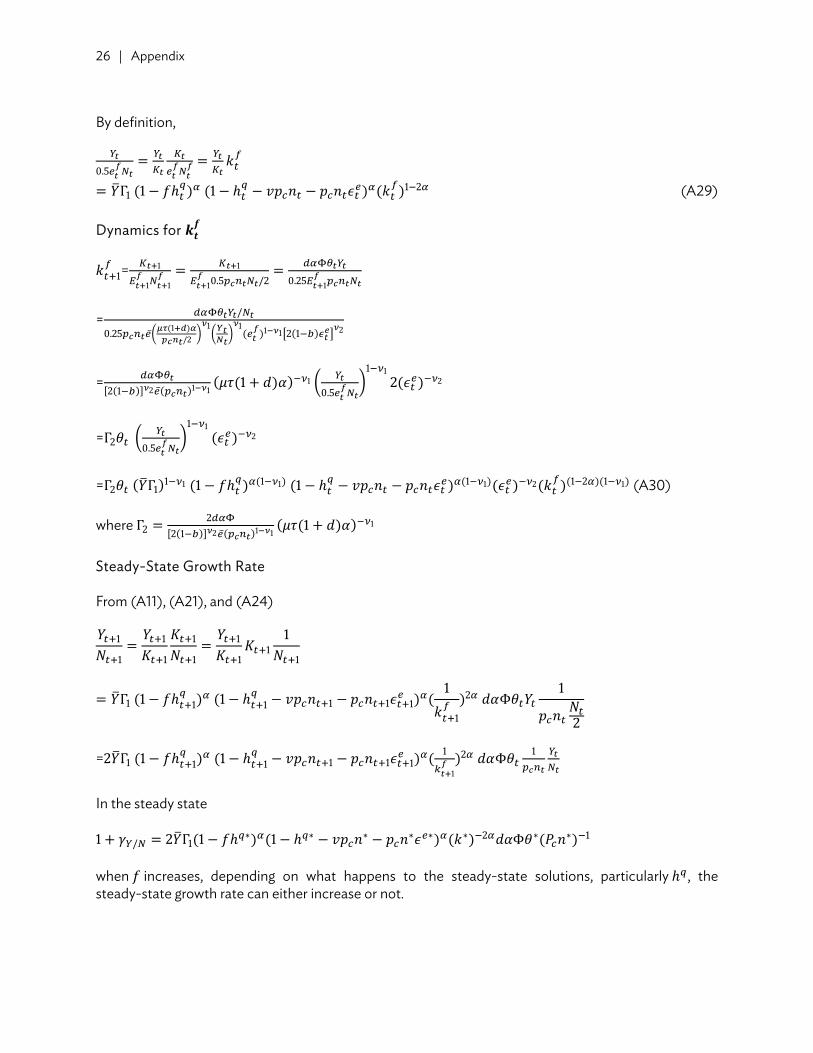
By definition,

.

Γ (A29) Dynamics for

=. / .

= /

. /

= .

=Γ .

=Γ Γ (A30) where Γ

Steady-State Growth Rate From (A11), (A21), and (A24)

Γ Φ

= Γ Φ

In the steady state

/ Γ ∗ ∗ ∗ ∗ ∗ ∗ Φ ∗ ∗ when increases, depending on what happens to the steady-state solutions, particularly , the steady-state growth rate can either increase or not.

REFERENCES Agénor, P. R. 2012. A Computable OLG Model for Gender and Growth Policy Analysis. University of

Manchester and World Bank. Unpublished. Agénor, P. R., and O. Canuto. 2013. Gender Equality and Economic Growth in Brazil: A Long-Run

Analysis. University of Manchester and World Bank. Unpublished. Barro, R. J., and J.-W. Lee. 1994. Sources of Economic Growth. Carnegie-Rochester Conference Series on

Public Policy. 40 (1): pp. 1–46. ————. 2013. A New Data Set of Educational Attainment in the World, 1950–2010. Journal of

Development Economics. 104. pp. 184–98. Becker, G. S. 1985. Human Capital, Effort, and the Sexual Division of Labor. Journal of Labor Economics.

3 (1). pp. S33–S58. http://www.jstor.org/stable/2534997?seq=1# page_scan_tab_contents Becker, G. S., and H. G. Lewis. 1973. On the Interaction between the Quantity and Quality of Children.

Journal of Political Economy. 81 (2). pp. S279–S288. Becker, G. S., K. M. Murphy, and R. Tamura. 1990. Human Capital Fertility and Economic Growth.

Journal of Political Economy. 98 (5). pp. S12–S37. Berik, G., Y. Rodgers, and J. Zveglich. 2004. International Trade and Gender Wage Discrimination:

Evidence from East Asia. Review of Development Economics. 8 (2). pp. 237–54. Berniell, M., and C. Sánchez-Páramo. 2011. Overview of Time Use Data Used for the Analysis of

Gender Differences in Time Use Patterns. Background paper for the World Development Report 2012.

Boserup, E. 1970. Women’s Role in Economic Development. New York, NY: St. Martin’s Press. Busse, M., and C. Spielmann. 2006. Gender Inequality and Trade. Review of International Economics. 14

(3). pp. 362–79. Cavalcanti, T. V. D. V., and J. Tavares. 2008. The Output Cost of Gender Discrimination: A Model-

Based Macroeconomic Estimate. Proceedings of the German Development Economics Conference, Zürich 2008, No. 43.

Cuberes, D., and M. Teignier. 2012. Gender Gaps in the Labor Market and Aggregate Productivity.

Working Paper. Department of Economics, University of Sheffield. http://eprints.whiterose .ac.uk/id/eprint/74398

————. 2014. Gender Inequality and Economic Growth: A Critical Review. Journal of International

Development. 26 (2). pp. 260–76. Dollar, D., and R. Gatti. 1999. Gender Inequality, Income and Growth: Are Good Times Good for

Women? Policy Research Report on Gender and Development Working Paper Series No. 1. Washington, DC: World Bank.

28 | References

Doepke, M., and M. Tertilt. 2009. Women's Liberation: What's In It for Men? Quarterly Journal of Economics. 124 (4). pp. 1541–91.

Duflo, E. 2010. Gender Inequality and Development? ABCDE Conference. Stockholm. May. Ehrlich, I., and F. T. Lui. 1991. Intergenerational Trade, Longevity, and Economic Growth. Journal of

Political Economy. 99 (5). pp. 1029–59. Elborgh-Woytek, K., M. Newiak, K. Kochhar, S. Fabrizio, K. Kpodar, P. Wingender, B. Clements, and G.

Schwartz. 2013. Women, Work, and the Economy. IMF Staff Discussion Note SDN/13/10. https://www.imf.org/external/pubs/ft/sdn/2013/sdn1310.pdf

Esteve-Volart, B. 2009. Gender Discrimination and Growth: Theory and Evidence from India.

Unpublished. Fernandez, R. 2009. Women’s Rights and Development. NBER Working Paper No. 15355.

http://dri.fas.nyu.edu/docs/IO/12607/DRIWP34.pdf Galor, O., and D. N. Weil. 1996. The Gender Gap, Fertility, and Growth. American Economic Review. 85

(3). pp. 374–87. Goldin, C. 1990. Understanding the Gender Gap: An Economic History of American Women. New York,

NY: Oxford University Press. Greenwood, J., A. Seshadri, and M. Yorukoglu. 2005. Engines of Liberation. Review of Economic Studies.

72 (1). pp.109–33. Hsieh, C. T., E. Hurst, C. I. Jones, and P. J. Klenow. 2013. The Allocation of Talent and US Economic

Growth NBER Working Paper No. 18693. http://www.nber.org/papers/w18693 Kim J., J.-W. Lee, and K. Shin. 2015. Gender Equality and Economic Growth in Korea. Korea University

working paper. Klasen, S. 2002. Low Schooling for Girls, Slower Growth for All? Cross-Country Evidence on the Effect

of Gender Inequality in Education on Economic Development. World Bank Economic Review. 16 (3). pp. 345–73.

Klasen, S., and F. Lamanna. 2009. The Impact of Gender Inequality in Education and Employment on

Economic Growth: New Evidence for a Panel of Countries. Feminist Economics. 15 (3). pp. 91–132.

Lagerlof, N. P. 2003. Gender Equality and Long Run Growth. Journal of Economic Growth. 8 (4). pp.

403–26. Organisation for Economic Co-operation and Development (OECD). 2012. Closing the Gender Gap:

Act Now. http://www.oecd.org/gender/closingthegap.htm Seguino, S. 2000. Gender Inequality and Economic Growth: A Cross-Country Analysis. World

Development. 28 (7). pp. 1211–30.

References | 29

Steinberg, C., and M . M. Nakane. 2012. Can Women Save Japan? IMF Working Paper No. 12/248.

https://www.imf.org/external/pubs/ft/wp/2012/wp12248.pdf United Nations Educational, Scientific and Cultural Organization (UNESCO). 2012. World Atlas of

Gender Equality in Education. http://www.uis.unesco.org/Education/Documents/ unesco-world-atlas-gender-education-2012.pdf

World Bank. World Development Indicators. http://data.worldbank.org/data-catalog/world

-development-indicators ————. 2012. World Development Report 2012: Gender Equality and Development.

https://openknowledge.worldbank.org/handle/10986/4391


AsiAn Development BAnk6 ADB Avenue, Mandaluyong City1550 Metro Manila, Philippineswww.adb.org

A Model of Gender Inequality and Economic Growth

This paper introduces a model of gender inequality and economic growth. The model is calibrated using microlevel data of Asian economies, and numerous policy experiments are conducted to investigate how various aspects of gender inequality are related to the growth performance of the economy. The analysis shows that improving gender equality can contribute significantly to economic growth by changing females’ time allocation and promoting their accumulation of human capital.

About the Asian Development Bank

ADB’s vision is an Asia and Pacific region free of poverty. Its mission is to help its developing member countries reduce poverty and improve the quality of life of their people. Despite the region’s many successes, it remains home to the majority of the world’s poor. ADB is committed to reducing poverty through inclusive economic growth, environmentally sustainable growth, and regional integration.

Based in Manila, ADB is owned by 67 members, including 48 from the region. Its main instruments for helping its developing member countries are policy dialogue, loans, equity investments, guarantees, grants, and technical assistance.

adb economicsworking paper series

NO. 475

February 2016

A MODEl Of GENDEr INEquAlIty AND EcONOMIc GrOwthJinyoung Kim, Jong-Wha Lee, and Kwanho Shin