Finance and Economics Discussion SeriesDivisions of Research & Statistics and Monetary Affairs

Federal Reserve Board, Washington, D.C.

A Model of Endogenous Loan Quality and the Collapse of theShadow Banking System

Francesco Ferrante

2015-021

Please cite this paper as:Francesco Ferrante (2015). “A Model of Endogenous Loan Quality and the Col-lapse of the Shadow Banking System,” Finance and Economics Discussion Se-ries 2015-021. Washington: Board of Governors of the Federal Reserve System,http://dx.doi.org/10.17016/FEDS.2015.021.

NOTE: Staff working papers in the Finance and Economics Discussion Series (FEDS) are preliminarymaterials circulated to stimulate discussion and critical comment. The analysis and conclusions set forthare those of the authors and do not indicate concurrence by other members of the research staff or theBoard of Governors. References in publications to the Finance and Economics Discussion Series (other thanacknowledgement) should be cleared with the author(s) to protect the tentative character of these papers.

A Model of Endogenous Loan Quality and the Collapse of the

Shadow Banking System∗

Francesco Ferrante †

Federal Reserve Board

First version August 2013

This version: March 2015

Abstract

I develop a macroeconomic model with a financial sector, in which banks can finance risky

projects (loans) and can affect their quality by exerting a costly screening effort. Informational

frictions regarding the observability of loan characteristics limit the amount of external funds

that banks can raise. In this framework I consider two possible types of financial intermediation,

traditional banking (TB) and shadow banking (SB), differing in the level of diversification across

projects. In particular, shadow banks, by pooling different loans, improve on the diversification

of their idiosyncratic risk and increase the marketability of their assets. Due to their ability to

pledge a larger share of the return on their projects, shadow banks will have a higher endogenous

leverage compared to traditional banks, despite choosing a lower screening level. As a result, on

the one hand, the introduction of SB will imply a higher amount of capital intermediated. On

the other hand it will make the economy more fragile via three channels. First, by being highly

leveraged and more exposed to risky projects, shadow banks will amplify exogenous negative

shocks. Second, during a recession, the quality of projects intermediated by shadow banks will

endogenously deteriorate even further, causing a slower recovery of the financial sector. A final

source of instability is that the SB-system will be vulnerable to runs. When a run occurs,

shadow banks will have to sell their assets to traditional banks, and this fire sale, because of

the limited leverage capacity of the TB-system, will depress asset prices, making the run self-

fulfilling and negatively affecting investment. In this framework I study how central bank credit

intermediation helps reduce the impact of a crisis and the likelihood of a run.

Keywords: Financial Frictions, Shadow Banking, Bank Runs, Unconventional Monetary Policy

JEL classification: E44, E58, G23, G24

∗The views expressed in this paper are those of the author and do not necessarily reflect the views of the FederalReserve Board or the Federal Reserve System. I am indebted to Mark Gertler, Jaroslav Borovic̆ka and Douglas Galefor their guidance in the preparation of this paper. I would also like to thank Andrea Prestipino for the very usefuldiscussions, and John Roberts and NYU seminar partecipants for their comments†Federal Reserve Board, francesco.ferrante@frb.gov

1 Introduction

The years leading to the 2007-2009 �nancial turmoil in the United States were characterized by the devel-

opment of a new set of �nancial institutions that formed the so-called "shadow banking" (SB) system. A

precise and all-encompassing de�nition of shadow banking is di¢ cult to obtain, but it can broadly be char-

acterized as a network of �nancial subjects that replicated the credit intermediation process by decomposing

it in di¤erent activities while heavily relying on securitization and sophisticated �nancial products.1

These entities included, for example, broker-dealers, mortgage �nance �rms, asset-backed commercial

paper (ABCP) conduits and money market mutual funds (MMMF), and provided an alternative chain

of intermediation, parallel to the "traditional banking" (TB) o¤ered by conventional banks. Simplifying

considerably the complex structure of the shadow banking system, we can provide an example of the basic

steps of the intermediation process as follows. Loans originated by non-bank lenders were pooled through

securitization by a loan warehouse vehicle, for example a special purpose vehicle (SPV) supported by a

broker-dealer.2 The broker-dealer further combined such loans into structured asset backed securities (ABS)

that were funded by issuing risk-free short term debt like commercial paper. MMMFs purchased the ABCP

and �nanced themselves with money-like securities with stable net-asset value. As a result, we can think of

the aggregate shadow banking system as engaging in the same maturity and liquidity transformation typical

of traditional banks, converting illiquid loans into demandable instruments.

If, on the one hand, this �nancial system increased the amount of credit available to borrowers, on the

other hand it proved to be inherently more fragile because of a series of risks a¤ecting its business model. In

this paper, I will focus on the following factors that increased the instability of the shadow banking system:

high leverage, moral hazard in selecting the riskiness of loans, and exposure to bank runs. In addition, this

paper will show how these channels can be ampli�ed by the interaction with traditional banks, which are

characterized by a lower leverage capacity.

Shadow banking, became more and more important in the years leading to the crisis. By 2007 the SB-

system was intermediating a volume of credit comparable to that provided by traditional banks.3 Figure

(1) provides an approximate measure of the SB-system, based on Pozsar et al (2010), considering all the

liabilities linked to "non-traditional" intermediation (like ABS, commercial paper, repos, MMMF shares).4

Di¤erent explanations have been given for this trend, including regulatory arbitrage or an increasing

demand for riskless assets. Nonetheless, an important factor behind the fast growth of shadow banking can

be clearly identi�ed in �nancial innovation. In particular, the securitization process, based on combining

di¤erent loans into diversi�ed portfolios, increased the marketability of banks�assets. As a result, by broad-

ening the array of securities available for lenders, shadow banks were able to create a new stream of outside

funding. Also for this reason, they had a higher leverage capacity than traditional banks.

Even if the SB-system helped to expand credit and lower borrowing costs in the period preceding the

�nancial crisis, it also played a crucial role in making the whole banking sector more fragile and in causing

1A survey of the di¤erent de�nitions and measurements of the Shadow Banking system can be found, for example, in theIMF Global Financial Stability Report of October 2014

2For example mortgage companies or �nance companies.3Private sector estimates of size vary from $10 trillion to $30 trillion (see Deloitte, 2012). A "Shadow Bank Index" developed

by Deloitte put its size in the U.S.at $20 trillion in 2007. Assets intermediated by commercial banks in that period wereapproximately $10 trillion.

4The details on the data used can be found in Pozsar et al (2012), page8. Compared to Pozsar et al. I do not include GSEliabilities, since I want to focus on the part of the SB-system that did not have government sponsorship. In addition, theseentities went under government conservatorship in 2008. By also adding Freddie Mac and Fannie Mae the size of the SB-systemwould be even larger.

1

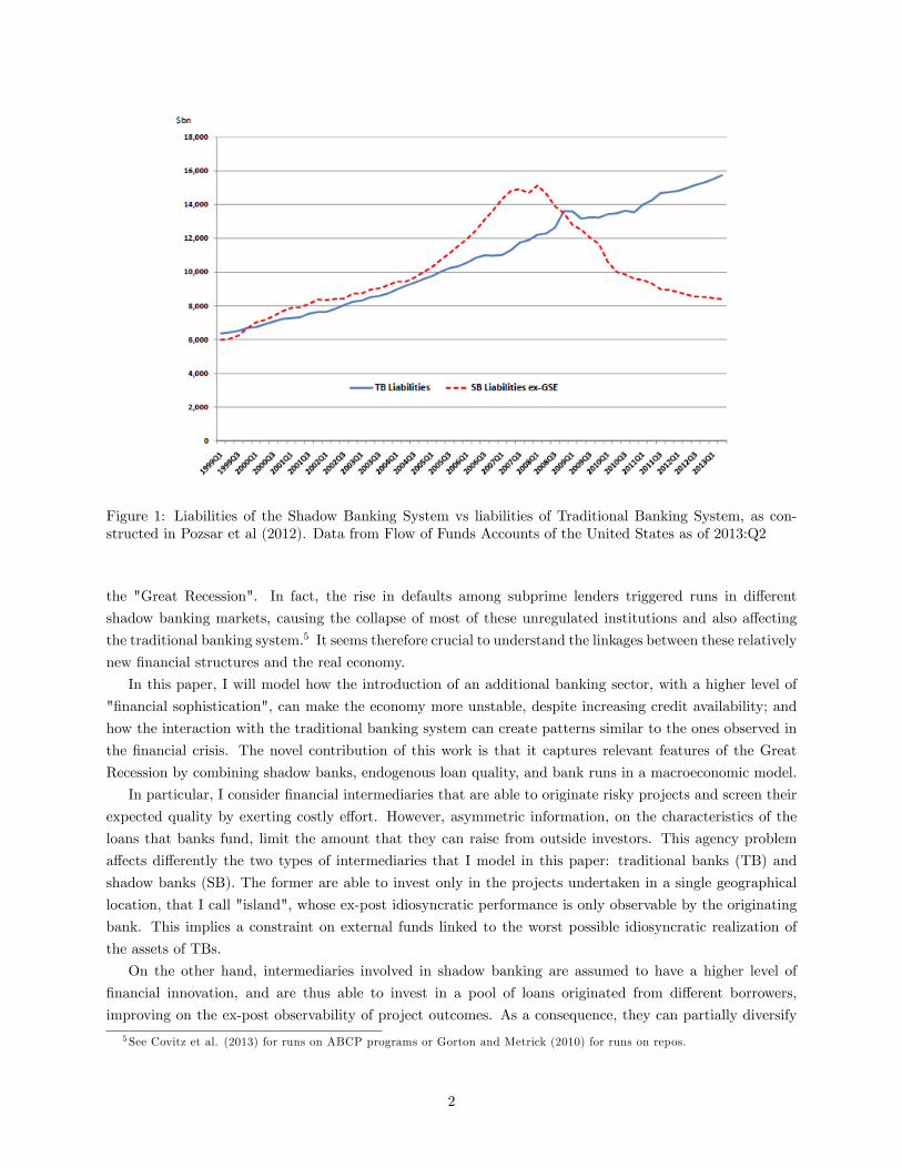
Figure 1: Liabilities of the Shadow Banking System vs liabilities of Traditional Banking System, as con-structed in Pozsar et al (2012). Data from Flow of Funds Accounts of the United States as of 2013:Q2

the "Great Recession". In fact, the rise in defaults among subprime lenders triggered runs in di¤erent

shadow banking markets, causing the collapse of most of these unregulated institutions and also a¤ecting

the traditional banking system.5 It seems therefore crucial to understand the linkages between these relatively

new �nancial structures and the real economy.

In this paper, I will model how the introduction of an additional banking sector, with a higher level of

"�nancial sophistication", can make the economy more unstable, despite increasing credit availability; and

how the interaction with the traditional banking system can create patterns similar to the ones observed in

the �nancial crisis. The novel contribution of this work is that it captures relevant features of the Great

Recession by combining shadow banks, endogenous loan quality, and bank runs in a macroeconomic model.

In particular, I consider �nancial intermediaries that are able to originate risky projects and screen their

expected quality by exerting costly e¤ort. However, asymmetric information, on the characteristics of the

loans that banks fund, limit the amount that they can raise from outside investors. This agency problem

a¤ects di¤erently the two types of intermediaries that I model in this paper: traditional banks (TB) and

shadow banks (SB). The former are able to invest only in the projects undertaken in a single geographical

location, that I call "island", whose ex-post idiosyncratic performance is only observable by the originating

bank. This implies a constraint on external funds linked to the worst possible idiosyncratic realization of

the assets of TBs.

On the other hand, intermediaries involved in shadow banking are assumed to have a higher level of

�nancial innovation, and are thus able to invest in a pool of loans originated from di¤erent borrowers,

improving on the ex-post observability of project outcomes. As a consequence, they can partially diversify

5See Covitz et al. (2013) for runs on ABCP programs or Gorton and Metrick (2010) for runs on repos.

2

the idiosyncratic risk and pledge a larger share of the return on their projects to outside lenders, by writing

contracts contingent on the realization of their pool of assets. In this way, shadow banks endogenously

achieve a higher leverage than traditional banks, so that the presence of the SB-system helps to expand

credit and to increase investments and output.

The �nancial sophistication of shadow banks, however, can be costly for the aggregate economy because

of the higher fragility of the �nancial sector. In this model such instability comes from three sources: higher

leverage, lower quality of loans, and the possibility of bank runs.

First of all, the higher aggregate leverage of the banking system will amplify negative exogenous shocks,

through a mechanism similar to the �nancial accelerator of Bernanke, Gertler and Gilchrist (1999) and

Gertler and Karadi (2011).

In addition, a novelty of this model is the interaction between asset quality and leverage, as a speci�c

feature of shadow banking: because the higher leverage is obtained by promising a higher payment to

investors in case projects are successful, shadow banks have a lower incentive to screen projects, and will

originate riskier loans. We can think of this as a stylized representation of the parallel boom of shadow

banking and subprime lending.

The moral hazard problem that links o¤-balance-sheet �nance and bank risk-taking represents one impor-

tant aspect of securitization, as shown in Pennacchi (1988) and Fender and Mitchell (2009). In addition to

being theoretically signi�cant, this characterization of shadow banking has received wide empirical support

in recent years. For example, Keys et al. (2010) �nd that securitized loans experienced higher default rates

than similar mortgages that were instead retained by the bank. Drucker and Puri (2009) show that �nancial

intermediaries usually sell riskier loans and provide covenants in order to reduce the problems arising from

information asymmetry. Su� (2007) shows that when borrowing �rms require more intense due diligence,

lenders retain a larger fraction of syndicated loans.

In this paper, I present a novel mechanism that shows the implications of this agency problem for the

cyclicality of bank asset quality. During recessions, as the value of shadow bank net worth declines, so does

their "skin in the game". As a result, the quality of the projects that the SB-system can credibly intermediate

will endogenously deteriorate even further, causing a slower recovery of this �nancial sector. On the other

hand, such a mechanism will be absent for traditional banks, since their funding capacity does not depend

on their screening e¤ort.

The evolution of asset quality will also translate in endogenous volatility in the cross-sectional equity

returns of �nancial intermediaries. In fact, during a crisis the volatility in the returns of �nancial intermedi-

aries, and in particular of shadow banks, will rise considerably, a type of countercyclicality that has received

great attention recently.6

Another important source of macroeconomic instability that a setup with two types of �nancial interme-

diaries allows me to consider is the eventuality of a run on shadow banks. In particular, because of their

high leverage and the type of securities they issue, shadow banks will be exposed to bank runs. On the other

hand, the low leverage and the incentive constraint on their liabilities rules out this possibility for traditional

banks. As a result, when a run occurs, shadow banks will have to sell their assets to traditional banks in

order to repay creditors, and this �re sale, because of the limited leverage capacity of the TB-system, will

depress asset prices and negatively a¤ect investment. If prices drop enough, the run becomes self-ful�lling

and most of the shadow banks are liquidated, causing a prolonged recession and a slow recovery of the

�nancial system.

6See, for example, Christiano, Motto, and Rostagno (2014); Ferreira (2014); Christiano and Ikeda (2014).

3

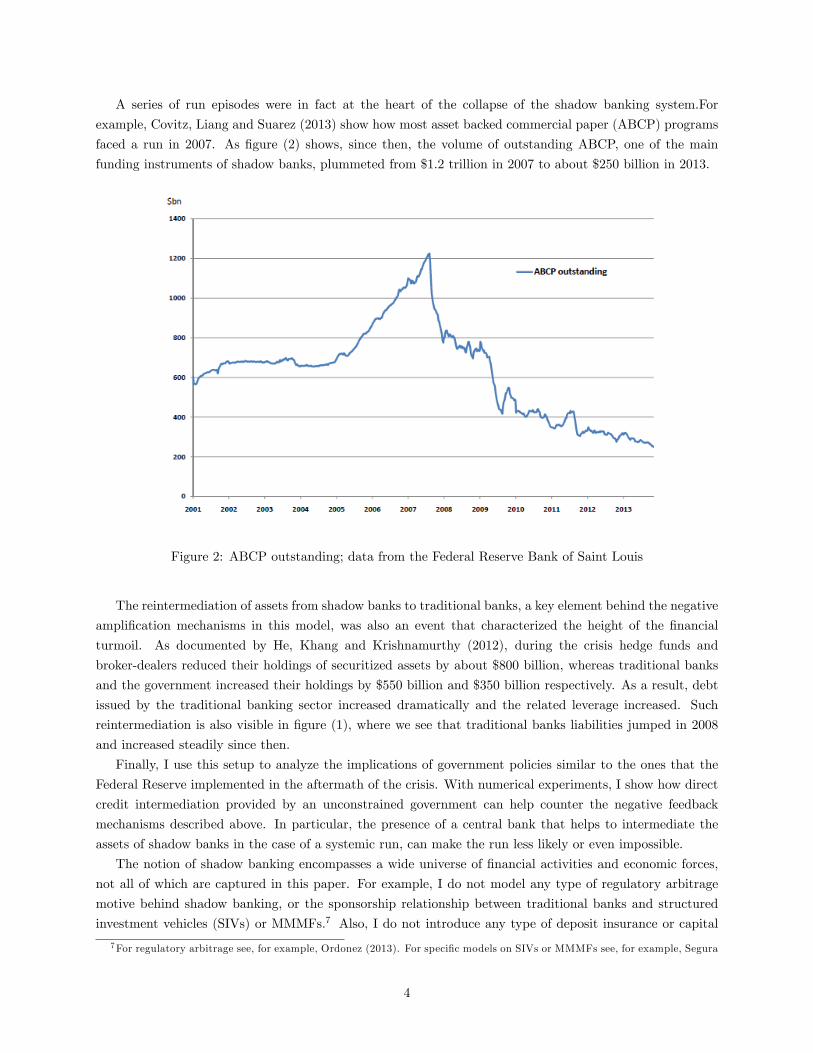
A series of run episodes were in fact at the heart of the collapse of the shadow banking system.For

example, Covitz, Liang and Suarez (2013) show how most asset backed commercial paper (ABCP) programs

faced a run in 2007. As �gure (2) shows, since then, the volume of outstanding ABCP, one of the main

funding instruments of shadow banks, plummeted from $1.2 trillion in 2007 to about $250 billion in 2013.

Figure 2: ABCP outstanding; data from the Federal Reserve Bank of Saint Louis

The reintermediation of assets from shadow banks to traditional banks, a key element behind the negative

ampli�cation mechanisms in this model, was also an event that characterized the height of the �nancial

turmoil. As documented by He, Khang and Krishnamurthy (2012), during the crisis hedge funds and

broker-dealers reduced their holdings of securitized assets by about $800 billion, whereas traditional banks

and the government increased their holdings by $550 billion and $350 billion respectively. As a result, debt

issued by the traditional banking sector increased dramatically and the related leverage increased. Such

reintermediation is also visible in �gure (1), where we see that traditional banks liabilities jumped in 2008

and increased steadily since then.

Finally, I use this setup to analyze the implications of government policies similar to the ones that the

Federal Reserve implemented in the aftermath of the crisis. With numerical experiments, I show how direct

credit intermediation provided by an unconstrained government can help counter the negative feedback

mechanisms described above. In particular, the presence of a central bank that helps to intermediate the

assets of shadow banks in the case of a systemic run, can make the run less likely or even impossible.

The notion of shadow banking encompasses a wide universe of �nancial activities and economic forces,

not all of which are captured in this paper. For example, I do not model any type of regulatory arbitrage

motive behind shadow banking, or the sponsorship relationship between traditional banks and structured

investment vehicles (SIVs) or MMMFs.7 Also, I do not introduce any type of deposit insurance or capital

7For regulatory arbitrage see, for example, Ordonez (2013). For speci�c models on SIVs or MMMFs see, for example, Segura

4

requirement for traditional banks, although the friction that I consider has the similar rationale of limiting

the leverage of traditional banks in order to guarantee that they are always able to repay depositors. The

modeling of all these phenomena is beyond the scope of this paper, whose focus is the interaction between

�nancial innovation, loan quality, shadow banking and macroeconomic instability.

1.1 Related Literature

This paper draws from di¤erent strands of literature related to agency problems in banking and their impli-

cations for the macroeconomy.

As regards the microfoundation for the limit on �nancial intermediaries leverage, my framework combines

a "worst-case-scenario" constraint, similar to the one used in Carlstrom and Samolyk (1995) and Bernanke

and Gertler (1987), with a moral hazard problem on monitored �nance, like the one modeled by Pennacchi

(1988) and Gorton and Pennacchi (1995). In particular, even if I do not model the details of securitization,

the contract between shadow banks and outside investors that I use is similar to the loan sales contract

described in these two papers.

An informational friction similar to the one used in this paper for shadow banks is used by Christiano

and Ikeda (2014): also in their model banks can a¤ect the probability of success of their projects by exerting

costly unobservable e¤ort. However, an important di¤erence comes from the fact that in their framework

the screening cost is not proportional to the amount of projects funded, so that no endogenous leverage

constraint arises from their agency problem. In such a framework the focus of their paper is rather to study

the possibility of improving welfare by introducing exogenous leverage restrictions.

Another paper in which the recovery of the �nancial sector is a¤ected by an endogenous deterioration in

asset quality is Bigio (2012). In Bigio (2012), this result stems from an adverse selection problem between the

bank and the borrower, in which the latter provides lower quality collateral as the volume of intermediation

shrinks. In addition, this mechanism is not the result of �nancial innovation, and a¤ects the banking system

as a whole, rather than being a speci�c feature of the shadow banking system.

My interpretation of shadow banking as a process to improve diversi�cation is similar to the one used by

Gennaioli et al. (2013). In their paper, banks can improve on their funding constraint by pooling di¤erent

assets in order to be able to pledge the worst aggregate realization on their loans, rather than the worst

idiosyncratic one. In their framework, shadow banking is driven by the demand for riskless assets by in�nitely

risk-averse depositors, and it becomes detrimental only when investors neglect tail risk. As mentioned in

the introduction, other papers have modeled shadow banking as stemming from regulatory arbitrage, like

Plantin (2012) or Ordonez (2013).

Recently many macroeconomic models with a �nancial sector have been developed (e.g. Gertler and

Karadi (2011), Brunnermeier and Sannikov (2011), He and Krishnamurthy (2012) ), but there have been

only a few attempts to include shadow banks and their exposure to runs in a general-equilibrium setting.

For example, Meeks et al. (2013) introduce in the framework of Gertler and Karadi (2011) a SB sector that

funds itself from traditional banks, and assume that traditional banks have a weaker friction when investing

in shadow bank liabilities. However, in such a setup, there is no role for loan quality and a run on the

SB-system, started by outside investors, is not possible. Faia (2012) studies the e¤ect of a secondary market

for loans in a DSGE model with a moral hazard problem similar to the one I consider, but where loan quality

is determined exogenously and only one type of intermediary is present.

(2014) or Parlatore (2013).

5

As regards the modeling of bank runs in general equilibrium, my approach is similar to the one used

by Gertler and Kiyotaki (2014). An important di¤erence is that in their paper, when a run occurs assets

are directly acquired by households that incur a real cost to manage capital. It is this cost that determines

the liquidation price and that makes a run possible. On the other hand, in my setup a run occurs because

of the �re sale of assets from shadow banks to traditional banks with a lower leverage capacity. Other

macroeconomic models of bank runs are Martin, Skeie, and Von Thadden (2012) and Angeloni and Faia

(2013).

The rest of the paper is organized as follows. Section 2 describes the asymmetric information problem in

the �nancial sector and the optimal contract for a �nancial intermediary operating as a traditional bank or

as a shadow bank. Section 3 presents the baseline model where both traditional banks and shadow banks

are present. Section 4 explains how a run on the shadow banking system is possible in this model. Section

5 shows a �rst set of numerical exercises with crisis experiments and run experiments. Section 6 introduces

government intervention and studies its interaction with �nancial crises and the possibility of a run. Finally,

Section 7 concludes.

2 Risky Projects and Financial Intermediaries

I begin by describing the agency problems a¤ecting the two types of �nancial intermediaries present in this

framework, and by solving the related optimal contracts. I then proceed to embed the �nancial system so

characterized in a medium-scale macroeconomic model.

One of the distinguishing features of banks in this model is that they are the only type of agent able

to invest in risky projects, by �nancing capital purchases of productive �rms. In particular, I assume that

there are two "regions", each with a continuum of �rms located on a continuum of islands.8 On every island,

�rms can invest in risky projects kt , or "raw capital", that will be employed in a constant-return-to-scale

production technology at time t+1.

Capital is risky because it can turn into �Hkt units of productive capital next period if the project

succeeds or �Lkt if the project fails, with �H > �L. Projects on a speci�c island will be perfectly correlated,

so that they either all fail or all succeed. However, I assume that the probability of success p di¤ers across

the two regions. In particular the two regions will be perfectly negatively correlated, so that every period one

region will be "good", whereas the other one will be "bad". The di¤erence between a region that turns out

to be good and one that instead is bad is in the probability of success of loans pG and pBt ; where pG > pBt .

Good �!(

�H w.p. pG

�L w.p. (1� pG)Bad �!

(�H w.p. pBt

�L w.p. (1� pBt )

Therefore, the proportion of islands with successful projects will be pG in the good region and pBt in the

bad one. In addition to assuming a higher probability of default in the bad region, I will also allow for iid

disturbances to pBt in order to capture, in a stylized way, a "subprime shock" that only a¤ects the return on

lower quality loans. De�ne the average realization of a project, conditional on the type of region as ��jfor

j = G;B, where��G= pG�H + (1� pG)�L and ��

Bt = pBt �H + (1� pBt )�L (1)

8An alternative interpretation is that of two "sectors". What is going to be important in the characterization of the setupis just the presence of a double layer of randomness in the outcome structure of projects.

6

It is important to stress that �nancial intermediaries are going to �nance projects in an island in a given

region at time t, without knowing whether that region will be good or bad at time t + 1, and whether

projects in a speci�c island will be successful or not. However, banks can exert e¤ort et in order to increase

the probability �t (et) of selecting a loan in a region that will be good next period. For simplicity I assume

that this probability is linear in e¤ort, according to �t = et, so that we can refer to �t also as screening level.

Imporantly, e¤ort is costly, since it entails a non-percuniary convex cost c(et) = c(�t), per unit of capital

intermediated. In particular I assume c (�t) = �2

��2t + ��t

�and I allow for � to be negative, meaning that

there could be some bene�ts from screening.9 However I consider calibrations where c0 (�t) > 0 meaning

that it is costly for �nancial intermediaries to increase their screening e¤ort.

We can de�ne the expected quality of a project with screening intensity �t as

Et [�t+1(�t)] = Et

h�t��

G+ (1� �t) ��

Bt+1

i(2)

Importantly, banks cannot perfectly diversify across all islands. This limit to diversi�cation implies

that the assets intermediated by each bank are risky and, as it will be clear below, it allows asymmetric

information on bank portfolios to create a relevant agency problem.

In addition, as I mentioned in the introduction, I consider two types of intermediaries, traditional banks

and shadow banks, di¤ering in the ability to diversify across islands. In particular I assume that TBs are

only able to invest in projects in one single island, that next period will deliver �H units of productive capital

in case of success and �L in case of failure. On the other hand, SBs are able to invest in a "pool" of loans

located in the same region. As a result, the outcome of the shadow bank�s portfolio will be either ��Gif the

region is good or ��Bt+1 if it is bad.

This framework is equivalent to one in which shadow banks purchase loans originated by a set of tra-

ditional banks located in the same region.10 As long as these loans are purchased at their market value,

implying zero pro�ts for the TB on these projects, the structure of the model would be identical. What I

am trying to model in this way, is the practice of pooling mortgages that was behind the rapid development

of securitization and the shadow banking system.

It needs to be noticed that even if SBs are more diversi�ed than TBs, they will still be exposed to some

idiosyncratic risk. As a supporting piece of evidence for this assumption, we can think of the fact that

securitized products mainly comprised loans belonging to a single asset class (credit-cards, mortages student

loans etc.), hence being far from perfect diversi�cation.

The di¤erent level of diversi�cation will play an important role in determining the funding constraints

for the two types of �nancial intermediaries because of two layers of information asymmetries:

1. Unobservable Outcome (UO):

� the default realization of loans (�L; �H), on a given island, is only observable by the originatingbank

� the type-realization of a speci�c region (good or bad) is public information.

2. Unobservable E¤ort (UE): the screening level of the loans that a bank funds (�jt for j = tb; sb) is

private information9The theoretical results of the paper hold for a generic quadratic cost function c (�t) = �

2

��2t + ��t + "

�, but the speci�c

form used has the advantage of providing a closed form solution for the optimal �t chosen by each type of intermediary.10With this interpretation the �t chosen by shadow banks would represent the probability of purchasing projects from

traditional banks located in a good region.

7

As a consequence of the di¤erent diversi�cation abilities of the two intermediaries, the �rst friction (UO)

will characterize the contracting problem between households and TBs whereas the second one (UE) will be

at the core of the funding constraint for the SB system.11

The crucial distinction between the two types of contracts will depend on the observability of the ex-post

realization of the loan portfolio held by each intermediary. In fact, because of the UO-friction, TBs can

credibly commit only to a payment linked to the worst possible realization of their projects. On the other

hand, since the outcome of their pool of loans is veri�able, SBs will be able to write a contract contingent

on the idiosyncratic realization of their assets. We can think of this framework as capturing the idea that,

by combining several loans, shadow banks created securities that were easier to evaluate for a rating agency

and hence easier to pledge to external investors.12

In particular I will show that traditional banks will have a smaller endogenous leverage than shadow

banks. In addition, unlike the case for SB, the funding capacity of traditional banks will not depend on the

expected quality of the loans they hold.

The idea behind this setup is that of a SB system that, because of �nancial products that exploit risk

diversi�cation, is able to increase the marketability of bank loans and to improve on the capital constraints

a¤ecting the traditional banking system, hence intermediating funds with a lower level of net worth.

Given this characterization of the �nancial system, I will �rst derive the optimal contract for �nancial

intermediaries in a �rst-best scenario when no asymmetric information is present and both the outcome and

the riskiness of a project are observable. This will serve as a benchmark to identify the ine¢ ciencies arising

from the agency problems of the two types of banks.

I will then derive the optimal contract for a traditional bank and the one for a shadow bank. In the

baseline model, I will consider an economy where both types of intermediaries are present, as it was the case

for the U.S. economy in the years preceding the �nancial crisis. The focus of this model is not to provide

a speci�c economic mechanism to explain the growth of the shadow banking system, but rather to take its

existence, size and agency problems as given, in order to study its macroeconomic e¤ects.

2.1 The Optimal Contract in the Frictionless Economy

In this subsection I assume that there is no asymmetric information problem a¤ecting the banking sector. I

will refer to this scenario as the "Frictionless Economy" or "First-Best Economy".

Let Qt be the price of a unit of capital at time t, and Rkt+1 the return per unit of e¤ective capital at time

t+1. As I will explain in more detail below, I assume that �rms are competitive and that there is no agency

problem between banks and entrepreneurs. Therefore, a bank will �nance the total capital expenditures

ktQt faced by each �rm and will receive the risky return per dollar invested, �jRkt+1, for j = H;L, depending

on whether the speci�c project is successful or not.

At the beginning of time t, a bank enters the economy with an initial net worth nt and has to decide the

amount of projects to �nance kt and the screening intensity �t. The required amount of external funding

11As an additional technical condition, I assume that at the moment of signing the contract with a bank (CB or SB), theindividual household does not observe the distribution of �nancial intermediaries across the islands. Equivalently we can thinkthat bank receives funds before having selected the speci�c island(s) where to invest.This simply rules out that investors areable to perfectly foresee which sector is good by inferring the monitoring level selected by intermediaries.12 It has to be noted that here we are referring to ex-post observability. The ex-ante riskiness of loans, depending on �, will

still be unobservable also for shadow banks and will be behind the agency problem that a¤ects shadow banking funding.

8

provided by households will hence have to be

st = Qtkt � nt

In this instance, I assume that the bank has access to the most e¢ cient diversi�cation technology available

in the economy, that is the one used by shadow banks, which allows the �nancial intermediary to invest in

a pool of projects in a speci�c region. As a result, the optimal contract will specify a pair of payments to

outside lenders per unit of capital , bG;fbt+1 and bB;fbt+1 , contingent on whether the pool of loans is good or bad.

In particular, these payments will have to satisfy the following participation constraint for the household

Qtkt � nt � Et�t;t+1

h�fbt b

G;fbt+1 + (1� �

fbt )b

B;fbt+1

iQtkt (3)

where �t;t+1 represents the household stochastic discount factor, and �fbt is the screening level chosen in the

frictionless case.

In addition, I assume limited liability for the �nancial intermediary, so that for every realization of

projects outcome the payment to households cannot be larger than the assets available to the bank, that is

bG;fbt+1 � ��GRkt+1 (4)

bB;fbt+1 � ��Bt+1Rkt+1 (5)

As mentioned in the introduction, �nancial intermediaries are able to increase the probability of selecting

a good project, �t, by facing a non-pecuniary cost, c(�t), proportional to the value of the loans �nanced. In

particular, I assume c(�t) = �t2

��2t + ��

�,

To solve the optimal contract we have to maximize the following bank objective:

maxkt;�t;b

gt+1;b

ht+1

Qtkt

nEt�t;t+1

h�fbt

���GRkt+1 � b

G;fbt+1

�+ (1� �fbt )

���BRkt+1 � b

B;fbt+1

�i� c

��fbt

�osubject to (3), (4) and (5).

The objective function of the bank includes the expected return from the pool of projects, net of the

payments to outside creditors and the screening costs. In particular, given that the bank is owned by the

representative household, as will be explained in the next section, it discounts future pro�ts with the same

discount factor.

In the appendix, it is shown that the �rst order conditions of this problem imply the following

c0��fbt

�= Et�t;t+1 ��t+1R

kt+1 (6)

Et�t;t+1

nh�fbt��G+�1� �fbt

���Bt+1

iRkt+1 �Rt+1

o� c

��fbt

�= 0 (7)

where ��t+1 =���G � ��Bt+1

�and I used Et�t;t+1Rt+1 = 1.

Equation (6) determines how the screening e¤ort is optimally chosen in the frictionless scenario. It

equates the marginal cost of screening to the social marginal bene�t, which is given by the extra return

generated by good projects with respect to bad ones. In addition, equation (7) equalizes the expected return

on capital, net of the screening cost, to the risk-free rate. This is a standard no-arbitrage condition for a

model with perfect capital markets.

9

Combining these two equations we can determine the risk-adjusted return to capital Et�t;t+1Rkt+1, and

consequently the level of capital in the economy. In this frictionless scenario, if we focus on �rst order e¤ects,

this quantity will generally not move over time.13 On the other hand, as will become clear in the following

sections, when there is a binding agency problem equation (7) will not hold with equality, implying a positive

premium on the adjusted return to capital, a distinguishing feature of macroeconomic models with �nancial

frictions. In addition, the movements in this premium will be important for the cyclicality of investments

and , a unique feature of this model, asset quality.

In the �rst best contract, bG;fbt+1 and bB;fbt+1 are not uniquely determined; any pair of payments satisfying

(3), (4) and (5) would be admissible. Finally, it is important to notice that in this case bank net worth

does not play a role in determining aggregate demand for capital, and that the optimal contract does not

constrain the �nancial leverage �t = Qtkt=nt.

2.2 The Optimal Contract for Traditional Banks

Let us now consider the optimal contract for a �nancial intermediary operating with the traditional banking

technology. There is a continuum of traditional banks, each providing funds to non-�nancial �rms located

in one single island. Each traditional bank �nances the investment in its projects, Qtktbt , by using its own

net worth, ntbt , and by issuing liabilities stbt .

The balance sheet of a traditional bank will then be

Qtktbt = ntbt + s

tbt (8)

Because of the (UO) friction described above, traditional banks will be limited in the amount they can pledge

to repay depositors. In particular, similarly to Townsend (1979), the payment to lenders cannot be contingent

on the idiosyncratic realization of the loans, since this is not observable, so that bG;tbt+1 = bB;tbt+1 = btbt+1. In

addition, for the amount that traditional banks commit to repay to be incentive-compatible, this will have

to satisfy the following incentive constraint

btbt+1 � �LRkt+1 (9)

This constraint comes from the fact that households cannot observe whether the loans held by the

traditional bank have defaulted or not, hence, the only payment that can be enforced is linked to the

worst possible idiosyncratic realization, since in this case the bank would not have incentives to misreport.

Importantly, this "worst-case-scenario constraint" also guarantees that the traditional bank will always be

able to repay its creditors, which is why we can also refer to (9) as a "solvency constraint". A similar type

of funding constraint can be found in other papers such as Bernanke and Gertler (1987) and Carlstrom and

Samolyk (1995). In addition, also Gennaioli et al. (2012) use a similar limit on bank deposits, but in their

case it is motivated by extreme risk-aversion among depositors rather than by asymmetric information.

Notice that in this setup, if (9) binds, the return on stbt will be devoid of idiosyncratic risk but will be

exposed to aggregate risk. In this sense, we can think of stbt as including both deposits and other types of

non-risk-free securities, like preferred equity.14 The important aspect is that since the payment is going to

13This is true unless there is a shock to ��Bt+114 In particular, it can be shown that the payment implied by the optimal contract can be implemented as a combination of

risk-free debt, equity, and a bonus to bankers in case the project is successful.

10

be contingent on the aggregate price Qt, traditional banks will always be able to repay their creditors.15 In

addition, this result will also imply that they will not be exposed to bank runs.

The implied objective for the traditional bank is therefore

EtQtktbt f�t;t+1

h��tbt��G+�1� �tbt

���Bt+1

�Rkt+1 � btbt+1

i� c(�tbt )g

Finally, when solving for the optimal contract we also have to take into account the participation con-

straint (PC) that guarantees that creditors receive an appropriate return on their lending activity

stbt � Et�t;t+1btbt+1Qtk

tbt (10)

This is going to be the same relationship implied by households �rst order condition for the choice of

traditional banks securities.

Given these assumptions, the one period contract between the TB and households will have to solve

maxktbt ;�

tbt ;s

tbt ;b

tbt+1

EtQtktbt f�t;t+1

��t+1(�

tbt )R

kt+1 � btbt+1

�� c(�tbt )g

s.t btbt+1 � �LRkt+1 (IC)�

Qtktbt � ntbt

�� Et��t;t+1b

tbt+1Qtk

tbt (PC)

It can be shown that when the incentive constraint binds 16 , then the following will be true

Et�t;t+1��t+1(�

tbt )R

kt+1 �Rt+1

�� c(�tbt ) > 0

This inequality shows the presence of a wedge between the discounted return on borrowers assets and the

cost of funds (Rt+1), two values that were equal in the �rst best scenario. This is a classic result in models

with �nancial frictions, but in this framework it is enriched by the endogenous choice of asset quality.

The incentive constraint will also limit the amount of assets that traditional banks can intermediate by

implying a constraint on their leverage, �tbt =Qtk

tbt

ntbt, given by

�tbt �1�

1� �LEt�t;t+1Rkt+1� (11)

We can give an intuitive interpretation to this relationship. First of all, the leverage capacity is increasing

in the expected aggregate return to capital Et�t;t+1Rkt+1, since it increases the amount that can be credibly

promised to external investors. For the same reason, leverage will be higher the higher �L, the recovery

rate on defaulted projects. It is also important to notice that the debt capacity of traditional banks is not

directly linked to the riskiness of their loans, �tbt . This is a consequence of the fact that traditional banks

can only pledge the worst possible realization, independently from the outcome of their projects.

As a result, the �rst order condition on the screening level will determine �tbt in a similar fashion to what

15 It would be possible to slightly modify the assumptions of the agency problem in order to have the TB issuing risk-freedebt as well. For example one could assume that if the project fails it delivers a predetermined amount of goods �Lkt. Howeversuch feature would not add to the dynamics of the model and it would make the characterization of the contract less intuitive.In addition, a framework in which also TB issue risk-free securities would amplify all the mechanisms in this paper because ofa higher �nancial accelerator in the TB sector.16See appendix for a detailed solution of the contract.

11

occurred in the frictionless scenario, that is according to

c0(�tbt ) = Et�t;t+1 ��t+1Rkt+1 (12)

The intuition for this result is the following: since the payment to households does not depend on whether

the loan will be in a good or bad region, the traditional bank will retain all the exposure to the idiosyncratic

risk and hence it will equalize the marginal cost of monitoring to the expected social marginal bene�t,

given by the extra expected return that a good project delivers. In terms of the dynamics of traditional

bank monitoring, this equation will imply countercyclical movements in the quality of their loans, since in

recessions the marginal value of monitoring will be higher, due to a larger discounted expected return on

capital.

If we use the speci�c functional form for the cost function , from (12) we can directly obtain the optimal

level of �tbt set by the traditional bank as

�tbt =Et�t;t+1 ��t+1R

kt+1

� t� � t2� (13)

which also shows how �tbt is decreasing in the parameter a¤ecting the marginal cost of screening, given

by � t.

At this point, we can de�ne the return that households obtain after lending to traditional banks as

Rtbt = �LRkt

�tbt�1

�tbt�1 � 1(14)

From the equations above, we notice how both the leverage ratio and the screening intensity of traditional

banks only depend on aggregate quantities, allowing for an easy aggregation. In addition, equation (14)

implies that Rtbt only depends on aggregate variables.

2.3 The Optimal Contract for Shadow Banks

Shadow banks have access to the same screening technology of traditional banks. However, they can use a

special diversi�cation technology that allows them to "pool" projects within a single region. As described

above, the type-realization of a region, that is whether it is good or bad, is publicly observable, enabling

shadow banks to overcome the UO-friction that a¤ects the relationship between households and traditional

banks. However, since the diversi�cation is not complete, shadow banks will still be exposed to some

idiosyncratic risk. Because of this, it will be the unobservability of the monitoring e¤ort chosen, �sbt , coming

from the UE-friction, that will constrain the amount of funds that shadow banks can raise.

The shadow bank will fund its capital, ksbt ; by using its net worth and by issuing securities, ssbt . Its

balance sheet will then be

Qtksbt = nsbt + s

sbt (15)

Unlike the case for traditional banks, the contract between shadow banks and outside investors will

specify payments to the households, per dollar of loan, that are contingent on the realized type of the loan

pool, that is bjt+1 for j = G;B. Again, because of limited liability, we require

bj;sbt+1 � ��jt+1R

kt+1 for j = G;B (16)

12

Note that this setup has some similarities to the pooling and tranching that was behind securitization,

because we could interpret this contract as the shadow bank selling a contingent claim to the outcome of

its pool of loans in return for an amount ssbt , similarly to the notion of "loan sale" presented in Pennacchi

(1988).

The expected return for the shadow bank, including the non-pecuniary monitoring costs, will be given

by

Qtkt

nEt�t;t+1

h�sbt

���GRkt+1 � b

G;sbt+1

�+ (1� �sbt )

���BRkt+1 � b

B;sbt+1

�i� c

��sbt�o

(17)

Importantly, because of the UE-friction, the contract for SBs will be characterized by a moral hazard

problem with hidden action. In particular, this is due to the fact that the payment to investors depends on

the quality of the loans originated by the shadow bank, �sbt , which is unobservable by outsiders.

Therefore, an incentive constraint (IC), that guarantees that the shadow bank will select a given screening

level, will be required:

�sbt = argmax�sbt

nEt�t;t+1

h�sbt

���GRkt+1 � b

G;sbt+1

�+ (1� �sbt )

���BRkt+1 � b

B;sbt+1

�i� c

��sbt�o

(18)

In addition, because the simple way in which banks can a¤ect the loans return distribution satis�es the

"convexity-of-distribution-function" condition described in Hart and Holmstrom (1986), we can write the

(IC) in a more tractable way, by using the �rst order conditions of (18), that is

c0��sbt�� Et�t;t+1

h��t+1R

kt+1 �

�bG;sbt+1 � b

B;sbt+1

�i(19)

It has to be noted that such a constraint does not bind in the problem of TBs, since the payment that

they promise to outsiders does not depend on the idiosyncratic realization of their projects.

Finally, we have to consider the participation constraint for lenders, which guarantees that the household

obtains an expected return equal to the opportunity cost of its funds. As in Bernanke, Gertler, and Gilchrist

(1999), I assume that the shadow banker is willing to bear all the aggregate risk, guaranteeing a payment

to the lender that is equal to the risk-free rate in expectation.17 As a result the participation constraint will

imply restrictions on bG;sbt+1 ; bB;sbt+1 contingent on the realization of the aggregate shock, according to

Rt+1ssbt �

h�sbt b

G;sbt+1 + (1� �sbt )b

B;sbt+1

iQtk

sbt (20)

If we focus on a parametrization that allows for a value of bG;sbt+1 ; bB;sbt+1 satisfying (20) and (16) to exist

for any aggregate state,18 then the household can diversify the residual idiosyncratic risk by investing in

"mutual funds" that lend money to several shadow banks, and promise a rate of return equal to the risk-free

rate.19 Hence, in this framework we can think of the security ssbt , as ABCP or shares of a MMMF.

In this setup, shadow banks are hence retaining all the exposure to �uctuations in asset prices and default

rates, and they issue to the mutual fund a senior claim on the return from their loans. Such a con�guration

is in line with the idea that even with the development of the "originate-to-distribute" model, which marked

17This assumption is mainly made to capture the fact that most of the liabilities issued by the shadow banks, like ABCP,were short-term non-contingent debt, that exposed the system to runs.18As I will explain in Section 5, such condition will not hold in the case of a run on shadow banks. However, since the run is

an unanticipated event it does not enter the optimal contract.19 It is relevant to notice that, because of the UO-friction, diversi�cation across commercial banks does not alter the structure

of the contract, and its payments. This depends on the fact that households are only able to require the same individualpayment of �LRkt from all the CB located on di¤erent islands.

13

the growth of the shadow banking system, most of the risk remained inside the �nancial sector, as noted,

among others, by Acharya, Schnabl and Suarez. (2013). In addition, this will imply that when there is a

low realization of Rkt+1, bG;sbt+1 will have to rise, so that the banks with a good pool of loans will have to pay

a higher amount to households, diminishing their net worth. Such mechanism will play an important role in

all the quantitative experiments, including the run.

Importantly, all these considerations are valid only in the "no-run equilibrium". In fact, as I will explain

later in the paper, the economy will admit an alternative "run-equilibrium", in which the payment implied

by the liquidation price and (20) would be such that bGt+1 > ��Gt+1R

kt+1, thereby violating limited liability.

However, if we consider only unanticipated runs, this characterization for the optimal contract remains valid

in the baseline economy.

The problem of the shadow bank can therefore be written as

maxksbt ;�

sbt ;b

gt+1;b

bt+1

Qtksbt

nEt�t;t+1

h�sbt

���GRkt+1 � b

G;sbt+1

�+ (1� �sbt )

���BRkt+1 � b

B;sbt+1

�i� c

��sbt�o

s.t. Rt+1�Qtk

sbt � nsbt

��h�sbt b

G;sbt+1 + (1� �sbt )b

B;sbt+1

iQtk

sbt (PC)

c0��sbt�� Et�t;t+1

h��t+1R

kt+1 �

�bG;sbt+1 � b

B;sbt+1

�i(IC)

bG;sbt+1 � ��GRkt+1 (LLG)

bB;sbt+1 � ��BRkt+1 (LLB)

where the last two equations represent limited liability constraints for each idiosyncratic realization.

The �rst result that can be proved is that if the (IC) binds then it will be optimal to pay the bank only in

case the pool belongs to a good region, so that bB;sbt+1 =��Bt+1R

kt+1.

20 This result follows from the �nding (see

Hart and Holstrom (1986) ) that, in order to provide incentives to monitor, it is optimal to give the worst

possible punishment to the agent when the bad realization occurs. Therefore, the contract for the shadow

bank will imply that if the pool of loans reveals to be a bad one, the whole return will be given to creditors

and the shadow bank will default, resembling a risky debt contract.21 As a result, we can rewrite the (IC)

as

c0��sbt�� Et�t;t+1

h��GRkt+1 � b

G;sbt+1

iIn addition, if the (IC) is binding then it can be shown that the following inequalities must be true

Et�t;t+1

nh�sbt��G+�1� �sbt

���Bt+1

iRkt+1 �Rt+1

o� c

��sbt�> 0 (21)

c0(�sbt ) < Et�t;t+1 ��t+1Rkt+1 (22)

The �rst inequality is analogous to the one obtained in the problem for the traditional bank: also in this

case the incentive constraint implies that the discounted return on bank assets is larger than the cost of

funds.

In addition, the second inequality implies that, given the same Et�t;t+1 ��t+1Rkt+1, the quality of loans

originated by shadow banks will be lower than the one of traditional banks.22 This result comes from the

20Details for the solution of the optimal contract can be found in the appendix.21A similar result is derived in Pennacchi (1988), where the loan�s return density is a continuous function with bounded

support.22This will be the case in the baseline model, where both TB and SB operate and Et�t;t+1 ��t+1Rkt+1 only depends on

14

fact that, unlike the traditional bank, the shadow bank does not retain all the idiosyncratic risk coming from

the choice of �sbt . By being able to pledge a larger portion of the return on its loans, the shadow bank does

not internalize all the expected bene�ts from monitoring, that is Et�t;t+1 ��t+1Rkt+1. As a result it will have

lower incentives to screen its projects.

Furthermore, from the PC we obtain that

bG;sbt+1 =1

�sbt

�Rt+1

(�t � 1)�t

� (1� �sbt )��bRkt+1

�(23)

and by substituting the implied value of bG;sbt+1 in (19) we obtain that the (IC) imposes the following

leverage constraint for shadow banks

�sbt �1�

�sbt c0(�sbt )�

�Et�t;t+1�t+1

��sbt�Rkt+1 � 1

� (24)

where

�sbt =Qtk

sbt

nsbt

In this case �sbt is increasing in the total expected return on the pool of loans, whereas it is decreasing in

the expected payment due to the bank �sbth��GRkt+1 � b

G;sbt+1

i= �sbt c

0 ��sbt �. In particular, a very importantconsequence of (24) is that it implies a negative relationship between screening e¤ort and leverage for the

shadow banks. In fact, because of the moral hazard problem related to the unobservability of �sbt , in order

for the shadow bank to have incentives to exert a higher e¤ort, it will need to have more "skin in the game"

to internalize the bene�ts of a larger �sbt . This is accomplished by requiring that the bank covers a larger

share of the investment with its own net worth, implying a lower leverage. In fact, as equation (23) suggests,

a lower leverage implies a higher payment to the bank in case of success, consequently increasing its incentive

to screen projects, as shown in the (IC).

Equation (24) represents an important di¤erence from the model of Christiano and Ikeda (2014). Since

in their framework the screening e¤ort is not proportional to the amount of capital �nanced by the �nancial

intermediary, the unobservability of bank e¤ort does not imply any limit to the amount of debt that the

bank can raise. This comes from the fact that the screening cost is not increasing with the amount of loans

originated. As a result, in the unobservable e¤ort scenario of Christiano and Ikeda (2014) equation (21)

holds with equality and aggregate net worth does not directly a¤ect investments. On the other hand, as it

will be clear in subsequent sections, the interaction between loan quality, leverage constraints and net worth

will play a crucial role in determining the aggregate dynamics of the shadow banking system and of the

whole economy.

In addition, it can be shown that

�sbt > �tbt (25)

This can be easily seen by using (22) when comparing (24) with (11). The intuition is that, when the IC

binds, the pledgeable income per unit of capital of shadow banks, Et�t;t+1��t+1

��sbt�Rkt+1

�� �sbt c

0 ��sbt �will be larger than the one of traditional banks, �LEt�t;t+1Rkt+1. As a result, shadow banks need a lower

net worth to fund the same quantity of loans.

It has to be noted that, even if we assumed that also the type realization of a region was unobservable,

aggregate quantities.

15

shadow banks would still have a higher leverage. This comes from the fact that, because of diversi�cation,

the worst possible outcome for a pool of projects �nanced by a shadow bank would be ��Bt+1, which is greater

or equal than �L. Therefore, even if they had to face the same type of contract used by traditional banks,

shadow banks would still be able to promise a larger expected return to investors, thus obtaining a higher

leverage. From this perspective, the relationship between shadow banking and diversi�cation is similar to

the one presented in Gennaioli et al. (2012), where by diversifying among themselves banks are able to o¤er

a payment linked to the aggregate "worst case scenario" rather than to the idiosyncratic one. In addition to

this mechanism, my model also introduces endogenous screening performed by intermediaries and captures

a link between shadow banking and laxer lending standards, which will play an important role in the crisis

experiments shown in the next section.

The inverse relationship between leverage and screening will be crucial to determine the cyclicality of the

asset quality of shadow banks. In particular, �sbt will be determined by the following equation

�E�t;t+1 ��R

kt+1 � c0

��sbt�� �

�sbt c0 ��sbt �� c ��sbt � = �Et�t;t+1 �� ��sbt �Rkt+1 �Rt+1�� c ��sbt � ��sbt c00 ��sbt ��

(26)

implying

�sbt = '(Et�t;t+1Rkt+1) where

@'

@Et�t;t+1Rkt+1< 0 (27)

The quantity Et�t;t+1Rkt+1 can be interpreted as the "external �nance premium" de�ned by Bernanke,

Gertler, and Gilchrist (1999). As equation (21) shows, an increase in the discounted return to capital is

associated with a tightening of the incentive constraint, so that we can interpret equation (27) as a negative

relationship between the quality of shadow banks loans and the severity of their agency problem. In fact,

during a crisis the net worth of �nancial intermediaries is eroded, causing a decrease in capital demand, a

consequent drop in prices and an increase in leverage together with Et�t;t+1Rkt+1. As a result of the higher

leverage, the shadow bank will have a lower level of "skin in the game" in the projects that it originates, and

consequently it will be able to credibly commit to a lower level of �sbt . The relationship in (27) will play an

important role in the model dynamics. In fact, it will imply that when a negative shock hits the economy

the quality of the loans intermediated by shadow banks will deteriorate, causing a slower recovery for the

net worth of these intermediaries and their ability to invest. In addition, a lower aggregate quality will also

imply a lower level of productive capital and output, making recessions more persistent.

In particular, given the cost function c(�t) = �2 (�

2t + ��), I show in the appendix that we obtain

�sbt = 2Et�t;t+1

hRt+1 � �BRkt+1

i�E�t;t+1 ��Rkt+1 � �

2 �� (28)

As a result, also in this case it can be shown that both �sbt and �sbt only depend on aggregate quantities,

facilitating aggregation in the shadow banking sector.

At this point we can summarize the key di¤erences between traditional banks and shadow banks in this

model. First of all, shadow banks will have a higher leverage than traditional banks, achieved thanks to the

possibility of pledging a larger share of the expected return on their loans. The larger amount of funds per

unit of net worth that shadow banks can �nance, will however be used towards lower quality projects, since

�sbt < �tbt . Finally, the endogenous quality of loans, depending on �it for i = tb; sb, will move countercyclically

for traditional banks but procyclically for shadow banks. As we will see in the quantitative exercises, all

these features point to a shadow banking system much more sensitive to aggregate negative shocks.

16

2.4 Aggregation in the Financial System

In the baseline model I assume that both types of �nancial intermediaries are operating, each �nancing a

di¤erent set of projects.

As explained in detail in the next section, I follow Gertler and Karadi (2011) in assuming that each banker

belongs to one of a continuum of households. In the baseline model each household will have three types of

members: a worker, a traditional banker and a shadow banker. At the end of every period bankers (both

traditional and shadow) exit the economy with probability (1� �) and are replaced by an equal mass ofworkers that start their banking franchise with an initial endowment !j for j = tb; sb, according to whether

they become traditional bankers or shadow bankers. As is standard in models with �nancial frictions, the

exogenous exit probability is used to prevent net worth from growing inde�nitely because of the excess

returns ensuing from the agency problem.

As shown in (11) and (24), we can exploit the fact that the maximum leverage constraints are independent

of individual-speci�c factors to aggregate across the two �nancial sectors. In particular, if we de�ne N jt for

j = tb; fb as aggregate net worth, then the demand for capital in the traditional banking sector and in the

shadow banking sector will be determined by

QtKtbt = �tbt N

tbt

QtKsbt = �sbt N

sbt

Therefore, the total capital intermediated by the �nancial sector is given by

QtKt = �tbt Ntbt + �

sbt N

sbt

From the equation above, we notice that the overall asset demand by banks is going to be a¤ected by

variations in both N tbt and Nsb

t . In particular, given the higher leverage of shadow banks, aggregate capital

is going to be a¤ected more directly by �uctuations in the net worth of non-traditional intermediaries. In

addition, since �sbt and �tbt also depend only on aggregate variables, we can de�ne the aggregate e¤ective

capital availalble for each type of �nancial intermediary as

K̂jt = �t(�

jt�1)K

jt�1 for j = tb; sb

If we aggregate across surviving and entering bankers we can obtain the following evolution of the

aggregate net worth for the traditional banking sector and the shadow banking sector, which comprises

the retained earnings of surviving bankers, N jst, and the initial net worth of new entrants N

je , that is

N jt = N j

st +Nje for j = tb; sb

In particular, for each speci�c sector, surviving bankers�net worth will be given by the di¤erence between

the earnings on the assets held and the cost of the liabilities issued in the previous period, multiplied by the

share of surviving bankers �

N jst = �fQt�1K̂j

tRkt �R

jtS

jt�1g for j = tb; sb (29)

17

Here we see how net worth depends on the average quality of the loans that are originated in a speci�c

�nancial sector: �t(�jt�1) = �jt�1

��G+ (1 � �jt�1)

��Bt for j = tb; sb. First of all, the lower �it�1 is the more

exposed to "subprime shocks" to ��Bt the net worth will be. In addition, a drop in the screening level at time

t; will negatively a¤ect the earnings in the next period. Furthermore, because of the higher leverage and the

risk-free return on liabilities, Nsbt will drop much more in response to negative shocks, as we will see in the

next section.

On the other hand, the aggregate net-worth of new bankers will be simply given by their initial endowment

N je = (1� �)!j for j = tb; sb

In particular, the ratio between !tb and !sb, together with leverage ratios and spreads, will be useful to

determine the relative size of each �nancial sector in the steady state of the economy. From this perspective,

this model will be agnostic about what forces determined the growth of the shadow banking system, and it

will simply use a calibration where the relative size of this parallel �nancial system is comparable to that of

the traditional banking sector. 23

As suggested by Christiano and Ikeda (2014), this framework with endogenous probability of bank default

has also implications for the cross-sectional standard deviation of banks�equity returns. Given the binomial

structure of bank payo¤s, the standard deviation for banks�return per unit of net worth at time t is

~�jt+1 =h�jt

�1� �jt

�i:5� �jt

h���GRkt+1 � b

j;Gt+1

�����BRkt+1 � b

j;Bt+1

�ifor j = tb; sb

For traditional banks this quantity is simply

~�tbt+1 =��tbt (1� �tbt )

�:5�tbt ��t+1R

kt+1 (30)

where the �rst term is decreasing in �tbt as long as �tbt > :5, which will always be the case in the calibration

of the model.

On the other hand, for shadow banks, the fact that ��BRkt+1 � bBt+1 = 0 implies

~�sbt+1 =��sbt (1� �sbt )

�:5 � �sbt ���GRkt+1 � bG;sbt+1

�and by using (23) we can write

~�sbt+1 =

�(1� �t (et))�t (et)

�:5 h�sbt����sbt�Rkt+1 �Rt+1

�+Rt+1

i(31)

where the �rst term is decreasing in �sbt , while the second term is increasing in the spread between shadow

banks expected return on capital and the risk-free rate. Importantly, during a crisis both terms will increase.

In fact, as explained above, �sbt decreases when bank net worth deteriorates and spreads rise. As a result,

the agency problem of shadow banks will become more stringent, increasing the external �nance premium.

As can be seen from (31) these movements contribute to increase �sbt+1.

Finally, the cross sectional standard deviation on the return on equity for the whole �nancial sector will

23One possible way to endogenize this quantity might be to assume the presence of di¤erent costs to access the shadow bankingtechnology or the traditional banking one, in order to obtain endogenous initial in�ows from households in each �nancial sector.Such approach is beyond the scope of this paper, but could be used as a rationale to explain the growth of shadow banking asresulting from a decrease in the cost to access alternative �nancial products in the years leading to the �nancial crisis.

18

be given by

~�fint+1 =

"�NTBt

�Nt

�2 ��TBt+1

�2+

�NSBt

�Nt

�2 ��SBt+1

�2#1=2(32)

where �Nt = NTBt +NSB

t .

3 The Baseline Model

To capture the macroeconomic e¤ects of shadow banking, I introduce the two types of �nancial intermediaries

described above in a medium-scale real DSGE model. In the model there are �ve types of agents: households

(HH), non-�nancial goods producers, capital producers and two types of bankers: traditional bankers (TB)

and shadow bankers (SB).

Only the �nancial intermediaries are able to invest in productive capital by �nancing risky projects and

they also own a unique technology allowing them to screen the quality of these assets.24 Households can

only invest by lending funds to banks. We can think of the assumption of limited market participation for

households as a result of bankers technological advantage in evaluating loans.

Traditional banks and shadow banks have the same screening technology, but they di¤er in their "diver-

si�cation technology". In fact, as described in the previous section, I assume that intermediaries operating

via shadow banking are able to (partially) diversify across a pool of projects, making the ex-post realization

of their portfolio more easily observable and increasing the marketability of their assets.

3.1 Households

As in Gertler and Karadi (2011), I assume that there is a representative household with a continuum of

members of measure unity. Within each household there is a fraction fw of workers, a fraction f tb of

�traditional bankers" and a fraction fsb of �shadow bankers", where fw + f tb + fsb = 1. In addition, I

assume that the fractions of the two types of bankers are equal, so that f tb = fsb = f b.

Workers provide labor and return wages to the household. Each type of banker manages a �nancial

intermediary, performing the screening decision, and transfers positive dividends back to the household.

There is perfect consumption insurance across household members.

Households cannot directly invest in capital, and the only way in which they can save is by lending funds

to the two types of �nancial intermediaries. In particular, the relevant utility function for the worker is

logCt � �L1+�t+i

1 + �

where Ct represents consumption and Lt labor. On the other hand, bankers utility is given by

logCt � c��jt

�Qtk

jt for j = tb; sb

As a result, if we de�ne �� = fw�, we can write the utility of the representative household as

Et

1Xt=0

�t

"logCt � ��

L1+�t

1 + �� c

��tbt�QtK

tbt � c

��sbt�QtK

sbt

#24From now on I will use the words "projects", "capital" and "loans" interchangeably

19

As described in the previous section, the �nancial system o¤ers two types of securities to outside investors.

Shadow banks o¤er securities , Ssbt ; that pay a risk-free return, Rsbt+1 = Rt+1 in case a run on the SB-system

does not occur. Since I am modeling the variety of institutions that composed the SB-system as a single

entity, we can think of Ssbt as representing the set of instruments that allowed investors to channel funds into

this parallel banking sector. For example we can refer to asset backed commercial paper (ABCP) or shares

of money market mutual funds (MMMFS), that in normal times were perceived as basically risk-free assets.

What is important is that lenders are paid according to a "sequential service constraint", so that if shadow

banks do not have su¢ cient resources to repay all creditors, the latter have an incentive to withdraw their

funds as soon as possible. In the model, I assume that a run on the SB-system is a completely unanticipated

event, so that I can characterize the household problem and the subsequent optimal contracts with the

�nancial intermediaries as if households do not expect a run event to occur next period.

Traditional banks issue liabilities Stbt , that pay a return Rtbt+1 that is exposed to aggregate �uctuations.

Because of the structure of this security, traditional banks will always be able to repay the promised return

on Stbt . Even if I am not directly modelling a government-backed deposit insurance, the microfoundation for

the funding problem of traditional banks will endogenously imply that they are not exposed to a bank run.

The budget constraint for households is given by

Cht + Stbt + S

sbt = Rtbt S

tbt�1 +R

sbt S

sbt�1 +�t +WtLt (33)

where Wt represents real wage and �t are pro�ts derived from the ownership of capital-producing �rms.

The �rst order conditions for the choice of assets and and labor are given by

Et�t;t+1Rjt+1 = 1 for j = tb; sb (34)

C�1t Wt = ��L�t (35)

where �t;t+1 = � CtCt+1

.

3.2 Physical Setup

As was shown above, all the traditional banks will choose the same �tbt and all the shadow banks will choose

the same �sbt so that if we de�ne the aggregate capital �nanced by one �nancial sector at time t as Kjt for

j = tb; sb, then the e¤ective capital available for production in each �nancial system will be

K̂jt = �t(�

jt�1)K

jt�1 for j = tb; sb (36)

and consequently, aggregate e¤ective capital will be

K̂t = K̂tbt + K̂

sbt

After the idiosyncratic default realization, projects become homogeneous raw capital again. Therefore,

if we denote by It aggregate investment and by � the rate of exogenous physical depreciation, then the

evolution of aggregate capital Kt = Ktbt +K

sbt , will be given by

Kt = (1� �)K̂t + It (37)

20

In addition, it will also be useful to de�ne the following measure for aggregate screening �̂t, which weights

the monitoring level of each type of bank by the share of capital intermediated

�̂t = �tbtKtbt

Kt+ �sbt

Ksbt

Kt

Therefore, we can de�ne "aggregate quality" as

�̂t (�̂t�1) =K̂t

Kt�1

At this point, comparing this setup with that of Gertler and Karadi (2011), we can think of �̂t(�̂t�1)

as a way to endogenize the "capital quality shock" used in their paper, which a¤ects the amount of capital

available for production in every period.

3.3 Non-Financial Firms

In the model there are two types of non-�nancial �rms: goods producers and capital producers.

3.3.1 Goods Producers

Goods producers operate a Cobb-Douglas production function with e¤ective capital and labor, under perfect

competition. Since labor is perfectly mobile across islands we can write aggregate output Yt as a function of

aggregate productive capital, K̂t; and aggregate labor Lt

Yt = AtK̂�t L

1��t (38)

where � 2 (0; 1) and At is aggregate productivity.Given the e¤ective capital available for production, �rms choose labor in order to satisfy

Wt = (1� �)YtLt

(39)

so that we can de�ne gross pro�ts per unit of e¤ective capital as

Zt =Yt �WtLt

K̂t

= �Yt

K̂t

(40)

Firms �nance the purchase of capital/projects every period by obtaining funds from �nancial intermediaries.

As in Gertler and Karadi (2011), I assume that there are no frictions in the relationship between banks and

goods producers. Banks can perfectly observe the realization (�L; �H) of projects purchased by a �rm in

a given island and can e¢ ciently enforce contractual obligations with these borrowers. As a result, goods

producers can issue state contingent claims that are a claim to future returns from one unit of investments.

Because of perfect competition, the price of these securities will be the same price of investment goods Qt.

It is important to notice that, because of perfect labor mobility and constant returns to scale, we do not

need to keep track of the distribution of default shocks, and consequently of e¤ective capital, across islands.

This allows us to consider a return per loan for an individual bank that is linear in expected quality, that is

21

Et�t+1��it�Rkt+1 for i = tb; sb, where

Rkt+1 =Zt+1 + (1� �)Qt+1

Qt

3.3.2 Capital Producers

Capital producers create new capital by using the �nal good as input and face convex adjustment costs in

the gross rate of change in investment, f�

ItIt�1

�It, where f(1) = f 0(1) = 0 and f 00 () > 0. They sell new

"raw" capital to �rms in the di¤erent islands at the price Qt.

Given that households own capital producers, they choose It to maximize the following

maxI�

1X�=t

���t�t;�+1

�QtI� � I� � f(

I�I��1

)I�

�so that the price of capital will be determined by

Qt = 1 + f

�ItIt�1

�+

ItIt�1

f 0�

ItIt�1

�� Et��t;t+1

�It+1It

�2f 0�It+1It

�Pro�ts, arising out of the steady state, are redistributed lump sum to households.

3.4 Equilibrium in the Baseline Model without Runs

To close the baseline model (in which we abstract from government intervention and runs on the SB-system)

we need to specify the equilibrium in the labor market and the aggregate resource constraint. In particular,

labor demand and labor supply will be equalized if the following holds

C�1t (1� �)YtLt= �L�t

Aggregate output is divided between household consumption Ct, and investment expenditures It

Yt = Ct +

�1 + f

�ItIt�1

��It (41)

The exogenous processes for productivity At, and monitoring cost � t, each follow an AR(1) process

At = (1� �A)ASS + �AAt�1 + "At

� t = (1� �� )�SS + ��At�1 + "�t

whereas I assume that the default rate of bad loans pBt follows an i.i.d. process and is not correlated with

"At ; "�t .

4 A Run on the Shadow Banking System

In this framework, the possibility of having two types of �nancial intermediaries �nancing investment expen-

ditures can cause the occurrence of an alternative equilibrium characterized by a run on the shadow banking

22

system. In particular, in a run scenario, households stop rolling over their debt with existing shadow banks.

As a result, in order to repay their creditors, existing shadow banks have to sell their assets to traditional

banks and entering shadow banks. In particular, the latter start operating with their small endowment !sb

and no pre-existing debt, and hence are not exposed to runs in the period. If the �re-sale value of these

assets, arising from the re-intermediation towards banks with low leverage capacity (TB) or very low net

worth (entering SB), is low enough, a run equilibrium that wipes out existing shadow banks will be possible.

After the run occurs, new shadow banks will accumulate net worth until the economy slowly transitions back

to the steady state.

As in Gertler and Kiyotaki (2013), I assume that at time t� 1 the run is a zero probability event for theagents in the economy. At time t households will decide whether to continue to provide funds to the existing

shadow bankers or not. Therefore, the run equilibrium will exist together with the "normal" equilibrium in

which agents keep lending to shadow banks. For this reason the possibility of a run is not taken into account

when deriving the optimal contracts in section 2.

A run equilibrium will be possible if investors believe that, if all households stop providing funds to

shadow banks, then the SB-system might not be able to satisfy all its creditors. Therefore, if we assume

some type of sequential service on the repayments from shadow banks liabilities, then all households have

the incentive to withdraw their funds in order to avoid being left with nothing.

As noted earlier, given the contract structure for traditional banks, a run on the TB-system will never

be possible in this framework. By introducing some changes to the contractual framework we could also

allow for this event, however the focus of this paper is on studying a run phenomenon similar to the one

that occurred during the great recession, and that mainly a¤ected the shadow banking sector.25

4.1 Conditions for a Run

As a �rst step to characterize the run equilibrium, we can determine a threshold value for the price of capital�Qt, below which a run on shadow banks is feasible. In particular, the events of a run happen as follows. At

the beginning of time t, households decide whether to roll over their ABCP or not. If they choose to run, the

assets of all existing shadow banks are sold to the TB sector and to entering SBs, and the amount obtained

is transferred to households. De�ne Q�t as the liquidation price realized in this case. Then, a run will be

possible if the liquidation value of the assets of the SB system is smaller than the claim of creditors, that is

(Zt + (1� �)Q�t )�t(�sbt�1)Ksbt�1 < Ssbt�1Rt (42)

At the individual bank level, given the contract between shadow banks and households, condition (42) is

equivalent to having a return on capital in case of a run, Rk�t ; so low that the payment to households, bGt ,

implied by the participation constraint (20) would have to be higher than ��GRk�t , violating limited liability.

That is, a run is possible if the price of assets is so low that even the shadow banks with a good realization

for their pool of loans would not be able to repay creditors.

When the condition above is satis�ed, all investors have the incentive to run in order to avoid being left

with zero after the run occurs. Notice that equation (42) can be equivalently stated as the condition such

25For example we could assume that payments promised by the commercial banks depend on the price of the economy withouta run Qt, so that there could be the possibility for the net worth of commercial banks to turn negative as well.However, given the lower leverage of TBs and the high leverage capacity of SBs a TB-run scenario in which SBs continue

operating seems quantitatively unfeasible, unless we also introduce some type of costly technology that allows households todirectly invest in capital as in Gertler and Kiyotaki (2013).

23

that the aggregate net worth of the shadow banking system, not considering new entrants, becomes negative,

that is

(Zt + (1� �)Q�t )�t(�sbt�1)Ksbt�1 �Qt�1Ksb

t�1Rt < Nsbt Rt

By using the balance sheet and the leverage equation for shadow banks, we can rewrite this condition as

Q�t < �Qt

where �Qt =1

1� �

"Rt

�t(�sbt�1)

1� 1

�sbt�1

!Qt�1 � Zt

#(43)

From this relationship, we can analyze how the possibility of a run depends on di¤erent endogenous economic

variables. In particular, all the variables contributing to an increase in �Qt will increase the measure of states

in which a run is possible. Similarly to Gertler and Kiyotaki (2013), �Qt will be higher when the leverage of

shadow banks, �sbt�1, is higher. In addition, a feature unique to this setup is that �Qt will also be decreasing

in �t(�sbt�1), the average quality of loans intermediated by the SB-system. This means that if the quality

of the assets intermediated by shadow banks starts deteriorating then the possibility of a run will become

greater. Such mechanism might have played an important role in igniting the run on several components of

the shadow banking system as the foreclosure rate on subprime securities began to surge.

Alternatively, given �Qt and Q�t , we can characterize the possibility of a run by computing the recovery

rate on SB assets, that is

� t =�t(�

sbt�1)(Zt + (1� �)Q�t )Ksb

t�1Ssbt�1Rt

Consequently, if � t > 1 an ex-post run will not be possible. This quantity can also be interpreted as the

fraction of "alert" withdrawing depositors needed for a run to be possible.

We can now turn to the determination of the liquidation price, Q�t . As mentioned above, I assume that

at the time of a successful run, once the existing shadow banks are liquidated, only traditional banks and

entering shadow banks will be able to intermediate capital. It is important to note that, unlike Gertler and

Kiyotaki (2014), a run event does not entail any additional output cost, but will have real consequences

because of the drop in investments caused by the collapse of the shadow banking system. Given the features

of the run equilibrium, it is easy to characterize the economy when a run occurs. In fact, the only modi�cation

needed is to set the net worth of surviving shadow bankers to zero, so that

Nsb�t = Nsb

e = (1� �)!sb

As a result, at the time of the run, the shadow banking sector�s ability to intermediate funds will be

dramatically a¤ected, since its net worth will fall almost to zero. Consequently, if the run occurs during a

crisis, the traditional banking sector will have to absorb a substantially larger amount of capital compared

to an equilibrium in which a run does not materialize. This will be crucial for the drop in Qt that will make

a run possible. Moreover, a drop in the price of capital will also a¤ect the net worth of traditional banks,

making the liquidation price even lower and a run more likely.

24

5 Numerical Exercises

The quantitative exercises in this section are meant to illustrate how the introduction of the shadow banking

system makes the economy more fragile, compared to a framework where only TB operate, the Traditional

Banking Economy (TBE), or one where there are no informational asymmetries, the Frictionless Economy

(FE). The impulse responses provided are the non-linear perfect foresight paths of the economy, in order to

capture the non-linearities arising especially when the endogenous state variables move far from the steady

state levels, as it occurs when a run takes place.

5.1 Calibration

Table 1 reports the parameters used for the baseline model. Out of the �fteen parameters of the model,

the seven parameters pertaining to preferences and technology are fairly standard. I use a discount factor

� = :99, a utility weight on labor �� = 2 and a Frisch elasticity of 1. The capital share � is set at 0.36, the

exogenous depreciation rate is 2.5% and the elasticity of the price of capital to investments, given by f 00, is

set at 2.3.

The remaining parameters are speci�c to my model. I assume � = 0:9, which implies that the average

life of bankers is 10 quarters. In addition, I normalize pH = 1, and I calibrate the other seven parameters

speci�c to the banking sector, �L; �H ; pb; � ; �; !tb; !sb to hit the following targets: a shadow bank leverage of

12 compared to a leverage for traditional banks of 4; a level of �sb equal to 0.95 and �tb equal to 0.975; a

steady-state quarterly spread of the return of capital over the risk free rate of 40 basis points, an aggregate

quality �(�̂) equal to 1 (a normalization), and a share of aggregate capital intermediated by shadow banks

equal to .5 .

The values for �tb and �sb are meant to capture the di¤erence in leverage between traditional banks

(leverage around 10) and broker dealers (leverage above 30) in the period preceding the �nancial crisis. The

aggregate levels of leverage are below the actual ones for �nancial intermediaries because in this model banks

are directly investing in the equity of the goods producers, and non-�nancial �rms typically have a much

lower leverage.

The values for the screening levels are meant to capture a delinquency rate for the loans of traditional

banks, 1� �tb = 2:5%, similar to the delinquency rate of prime mortgages. On the other hand the implied

delinquency rate for loans originated by shadow banks is twice as large at 5%, and is a conservative estimate

of the delinquency rate of subprimes.26

Finally, the spread on the return on capital is supposed to be a combination of the average spread on

mortgage backed securities, around 100bp annually, and the Baa-treasury spread on corporate bonds, which

was larger than 2% annually.

Given these parameters, in table 2 I also report the implied steady state values for the "Frictionless

Economy" (FE), where �nancial frictions are absent, and the "Traditional Banking Economy" (TBE) where

the only type of �nancial intermediaries present are traditional banks.27 From table 2, we see how the

introduction of shadow banks increases capital (by 20%), output (by 8%) and consumption (by 3%) with

respect to the TBE, even if loan quality is lower. On the other hand the baseline economy implies lower

values for these variables, when compared to the frictionless one.

26Delinquency rates on adjustable rate mortgages (ARM) were above 10% in 2005.27 In particular, in this case I assume that the transfer to traditional banks is equal to the total transfer to the �nancial sector

in the baseline economy, that is !tbe = !tb + !sb.

25

In addition, if we measure these di¤erences in terms of the change in consumption that would equalize the

steady state utilities across the di¤erent economies, we have that the introduction of shadow banks provides

a consumption equivalent gain of 3.6% but it falls short of the frictionless economy by about .02%.28

5.2 Crisis experiments

In this set of examples I compare the response of the baseline economy (solid line), in the no-run equilibrium,

with the response of the traditional banking economy (red dashed line) and of the frictionless economy (green

dotted line) to the same shock.

As a �rst experiment, I consider a 1% drop in productivity with a persistence of 0.95. Figure (3) reports

the results for the di¤erent economies. In the baseline model, the drop in At negatively a¤ects the net worth

of both banks. As a result, because of the tightening in their balance sheet, banks will have to sell their

assets, depressing asset prices and further a¤ecting the net worth of �nancial intermediaries. This sequence

of events is in line with the �nancial accelerator mechanism described in Gertler and Karadi (2011) and

other macroeconomic papers with �nancial frictions. However, there are several aspects of a crisis that are

unique to this setup.

First, we notice that during the downturn, traditional banks�asset holdings increase by about 8%, whereas

projects funded by shadow banks decrease by about 12%. This is similar to the reintermediation of credit

that I have described in the introduction. In fact, because of their higher initial leverage, the decline in net

worth will make the �nancial constraint of shadow banks more binding, so that they will have to o­ oad assets

to the other �nancial sector. However, because of their lower leverage capacity, for traditional banks to be

able to absorb the capital held by shadow banks, prices need to adjust downward. This ampli�es the �nancial

accelerator channel, resulting in an initial drop in Nsbt of about 25%, and a prolonged reintermediation as

we can see from the evolution of Ktbt and Ksb

t in the graph. Consequently, aggregate investments and prices

decrease, causing a slower recovery of the capital stock in the economy.

An additional variable that is going to determine the recovery of the economy is the endogenous quality

of loans. As we can see in the bottom-right part of �gure (3), �sbt decreases by more than 7% on impact,

whereas �tbt increases by about 0.5%. As explained in section 2, these opposite movements are a consequence

of the di¤erent contract structures. Given the drop in prices and the higher expected return on capital,

traditional banks �nd it optimal to increase their screening e¤ort. On the other hand, the considerable

deterioration in shadow banks net worth decreases the "skin in the game" that they can credibly promise to

investors, implying a lower level of screening.

The lower quality of loans intermediated by shadow banks during a recession makes the crisis more

persistent for two reasons. First, it causes a slower recovery for Nsbt , because of the implied lower average

return in the shadow banking sector. In addition, since the drop in �sbt is larger than the increase in �tbt , the

"aggregate quality" of capital, �̂, deteriorates by about .3%. As a result, e¤ective capital falls, contributing

to a slower recovery of output.

Importantly, this e¤ect is basically absent when we consider the other two types of economy. If we

compare the path of the baseline economy with the TB economy and the Frictionless economy, we see that

the productivity shock has larger consequences when shadow banks are present. One reason for this is

the lower aggregate leverage in the economy with only traditional banks. This implies a weaker �nancial

28 It has to be noted that a proper welfare evaluation would require to solve the model globally accounting also for thefrequency of crises arising from the binding incentive constraints. However this is beyond the scope of this paper and is left forfurther research.

26

accelerator, as evidenced by the fact that the drop in prices is about 80% smaller than in the baseline

economy. In addition, in the traditional banking economy there is no deterioration in asset quality during

a recession. As a consequence, the net worth of traditional banks su¤ers a moderate drop and recovers

relatively quickly, and the decrease in aggregate capital and labor (not reported) is about one fourth of that

experienced in the baseline economy. The TB-economy behaves similarly to the frictionless economy because

of the low leverage and the absence of interaction between loan quality and funding capacity. However it

has to be remembered that, as shown in Table 2, the steady state values of consumption and output are

substantially lower in the traditional banking economy.

Next, I consider a "subprime shock" that a¤ects only the average quality of bad loans, ��Bt . In particular I

consider an increase in the default rate in the bad region (a decrease in pBt ), with no persistence, that causes

a 10% drop in ��Bt . We can think of this experiment as the initial rise in subprime defaults that ignited the

�nancial crisis.

The results of this experiment are reported in �gure (4). Given that bad loans represent only a small

portion of total projects, the drop in the aggregate quality of e¤ective capital at time t, �̂t is only .3%,

so that this can be considered as a relatively small "capital quality shock" as the one used by Gertler and

Karadi (2011) or Gertler and Kiyotaki (2010). In this case, the initial shock hits the net worth of shadow

banks more directly because of the higher exposure to bad projects. Once the �nancing conditions of banks

become tighter, we will have all the same mechanisms described in the previous experiment: the �nancial

accelerator, the reintermediation, and the deterioration of the quality of projects �nanced by the SB-system.

As a consequence, aggregate capital declines up to 1% so that output and consumption experience a prolonged

decline, despite the absence of persistence in the shock.

If we consider the responses in the traditional banking economy and the frictionless economy, we see that

the di¤erence from the baseline economy is even larger than in the previous experiment. First of all, the

initial impact on existing e¤ective capital is about 50% larger in the shadow banking economy, as can be

seen from the di¤erent drops in �̂t, because of the larger proportion of bad loans �nanced.

In addition, since the shock is i.i.d, this experiment captures in a stark way the slower recovery caused

by shadow intermediaries. In fact, in the economy with only traditional banks, the �nancial sector is more

stable both because of the lower leverage and because bank liabilities are contingent on the aggregate state.

Consequently, after the initial shock to N tbt , the economy is able to quickly restore capital by increasing

investments, so that prices are almost unchanged. As a result, at the trough, the drop in output and

consumption is less than one-tenth of the one occurring in the baseline economy.

Finally, �gure (5) presents the evolution of the cross-sectional volatily of equity returns in the �nancial

sector, for each shock. The �rst thing to notice is the spike in ~�sbt+1, which increases by 65% with the tfp

shock and 40% with the subprime shock. Looking at equation (31), we can see that this is due to three

e¤ects, all resulting from a deterioration in Nsbt : the drop in �

sbt , the increase in leverage, �

sbt ; and the higher

expected return from capital (due to the tightening of the incentive constraint).

On the other hand, ~�tbt+1 is characterized by a much smaller movement in the opposite direction, due to

the opposing movements in �sbt , �tbt and Et�t;t+1R

kt+1, as can be seen from equation (30). As a result, the

standard deviation in the whole �nancial sector increases in both experiments, as it occurred at the peak of

the �nancial crisis.

27

5.3 An Increase in the Screening Cost

After analyzing how the di¤erent banking systems react to real disturbances, we can now focus on shocks

that directly interact with the nature of the �nancial frictions. Figure (6) shows the e¤ect of an unanticipated

5% increase in the variable � t, which implies a higher marginal cost of screening projects for both banks,

with a persistence of .5.

As can be seen from (13) and (28), the immediate e¤ect of such a shock is a drop in both �tbt and �sbt ,

due to the fact that monitoring is now more costly for banks. In the TB-system this is the only e¤ect that

takes place.

However, in the shadow banking system, the higher cost of monitoring will also make the UE-friction

more severe, because now the cost to provide incentives to bankers will be higher. This will imply a negative

pressure on the maximum leverage constraint for shadow banks, as described in (24), so that shadow banks

will have to start selling their assets. As a result, spreads will increase and current prices will drop generating

all the ampli�cation e¤ects described in the previous experiments. The interaction of � t with shadow banks

leverage implies that �sbt drops about 1% more than �tbt . In addition, the recovery in aggregate quality is

slower in the baseline model, because it is also driven by a slower recovery of prices.

Interestingly, even if this shock does not have any real consequences on impact, it causes output and

consumption to drop up to 0.3% and consumption up to .4% . In the traditional banking economy, the only

e¤ect comes from the initial drop in �, which however quickly returns to the steady state level, since prices

and investments stay almost unchanged. As a result, output experiences a contraction 50% smaller than in

the baseline model.

5.4 A Wealth Transfer Within the Financial System

In order to illustrate the relevance of the di¤erent leverage capacities of the two �nancial sectors and the

consequences of reintermediation, I consider a simple experiment in the baseline model that consists in a

transfer from the net worth of shadow banks to the one of traditional banks. In particular, �gure (7) shows

the e¤ects of a transfer T equal to 1% of the steady state level of Nsbt .

Given the lower leverage of traditional banks, the amount of funds that can be intermediated with T

units of internal funds is lower in the traditional banking sector than in the shadow banking one. As a result,

aggregate investments decline igniting a drop in prices and the consequent ampli�cation mechanisms present

in the baseline model, implying �re sales and a decline in aggregate loan quality. Given the drop in Qt, the

actual initial drop in Nsbt is actually larger than 1%.

The real e¤ects of reintermediation will play an important role in the run experiment that I consider in

the next subsection.

5.5 A Run Experiment

During the �nancial crisis, investors stopped considering some of the securities issued by the shadow banking

system as substitutes for risk-free assets. This caused a run �rst on the ABCP market and then on the

MMMFs. To model the consequences of these events, I now allow for the possibility of a run on the shadow

banking system.

Given the liquidation price, Q�t , and the threshold, �Qt, determined in (43), a run will be possible in the

baseline model at time t if and only if

Runt = �Qt �Q�t > 0

28

The model calibration implies that a run equilibrium is not possible in steady state. However, during a

recession �Qt will increase and Q�t will decrease, so that the quantity Runt will indicate whether a run is

feasible after a shock hits the economy.

First, I consider a run occurring after a tfp shock. In addition, in line with the narrative of the recent

�nancial crisis, I also consider the eventuality of a run happening after an increase in the default rate of

riskier loans. In particular, I consider the same shock magnitudes as in �gures (3) and (4).

Figure (10) shows how, after the initial shock is realized, a run becomes possible for four periods in both

cases. In �gure (8) and (9), I compare the path of the economy when the run happens in the third period

(the dashed red line) to the same response of the baseline economy (solid blue line) when a run does not

occur. Both lines are deviations from the steady state of the baseline economy.

When the run occurs, traditional banks absorb most of the capital of defaulting shadow banks. As a

result, the capital holding of traditional banks increases much more dramatically in this case. Due to the

low leverage capacity of traditional banks, in order for them to be able to intermediate such a higher amount

of capital, prices need to drop by almost 10%, instead of the much smaller drop that would have occurred

without a run. It is this drop in Qt that makes the run possible. At the time of the run, the net worth

of shadow banks drops by more than 95%, causing a much slower recovery for this �nancial sector. The

considerably larger decrease in asset prices and Nsbt implies a noticeable ampli�cation of all the feedback

mechanisms that I have described in the previous set of experiments. In fact, in both �gure 7 and �gure

8, after a run occurs investment drops by more than 10% and asset quality by more than 1.5%, implying

a decrease of output and consumption at the trough of more than 2%. In addition, the decrease in prices

negatively a¤ects the net worth of the surviving traditional banks, impairing their ability to invest and

further reducing prices. Interestingly, as �gure 9 shows, the possibility of a bank run can create a deep and

prolonged recession even after a relatively small shock like the subprime one.

In both cases, the initial increase in consumption occurring at the time of the run is due to the fact

that households are not able to invest in the TB-system all the funds that they have withdrawn from the

SB-system. This path for consumption is consistent with that observed during the �nancial crisis.

6 Government Intervention

In this section, I consider the possibility that the government is willing to facilitate lending by directly

purchasing securities in the asset market, similarly to some of the unconventional policies that the Fed put

in place during the �nancial crisis. De�ne the total amount of assets that are privately intermediated by the

�nancial sector as Kpt = Ktb

t +Ksbt . Therefore, if the government funds an amount K

gt ; the total value of

assets will be

QtKt = QtKpt +QtK

gt

The government can fund itself frictionlessly by issuing risk-free bonds, Dgt , but it does not have the moni-

toring technology owned by the banking sector. In particular, I assume that the government�s projects will

have a �xed quality ��. It is also important to assume that the goverment will be able to diversify also across

regions. On the other hand, as in Gertler and Karadi (2011), I assume that government intermediation

causes e¢ ciency costs proportional to the amount funded, �QtKgt .

If we de�ne Tt as government transfers, the government�s budget constraint will be

�QtKgt +QtK

gt +RtD

gt�1 = Dg

t +�t(��)RktQt�1K

gt�1 + Tt

29

and if we assume that at every period the government is going to fund its asset purchases through risk-free

bonds then Dgt = QtK

gt , so that we can rewrite the budget constraint as

�QtKgt = Tt +

��t(��)R

kt �Rt

�Qt�1K

gt�1

To characterize government policy, I assume that the central bank intermediates a fraction t of total

assets,

Kgt = tKt

To model t, I assume that the government intervenes when spreads�EtR

kt+1 �Rt+1

�rise. In fact, this

will occur during a crisis, when prices drop and �nancial frictions are tighter. In particular, I consider the

following simple rule for government intervention

t =

( 1�Et��t+1(��)R

kt+1 �Rt+1

�if�Et��t+1(��)R

kt+1 �Rt+1

�> 0

0 otherwise(44)

where I parameterize �� in such a way that Et��t+1(��)R

kt+1 �Rt+1

�is zero in the steady state of the baseline

model. This implies that �� < �sb < �tb. Therefore, the government will start intermediating assets only

when it makes a positive excess expected returnn. The parameter 1 will determine the intensity of the

government reaction.

6.1 Crisis Experiment with Government Intervention

Figure 11 and 12 show the response of the baseline economy to the same shocks considered in �gure (3)

and (4), when the credit policy is in place. The parameter 1 is set to 5 (or to 20), so that the government

intermediates 2% (or 3%) of assets when the tfp shock hits and 1.5% (2%) when the subprime shock occurs;

the ine¢ ciency parameter � is set for now at .0025.

By intervening in the asset market, the central bank initially prevents the reintermediation from shadow

banks to traditional banks. In this way, government intervention contains the drop in prices, causing a faster

recovery in the net worth of shadow banks and reducing the initial deterioration in asset quality. The impact

of central bank credit intermediation on the endogenous quality of assets is a novel mechanism of this paper,

highlighting an additional positive e¤ect of government intervention during a crisis. Under this policy, the

drop in output and consumption is up to 50% smaller at the trough than in the baseline model.

6.2 Run Experiment with Government Intervention

In this framework, it is interesting to investigate how government intervention interacts with the possibility

of a run. Even if the run is unanticipated, I can look at the fraction of "alert" investors, � t, necessary for a

run to be possible, as an indicator of the exposure of the economy to a run on the SB-system. In particular,

I assume that the government policy described above, is in place also in the run equilibrium. The idea

is that now, at the time of the run, investors know that the government will act in order to increase the

leverage capacity of the �nancial system, whether this is composed only of traditional banks or of both types

of �nancial intermediaries.

In �gure (13) I consider the same run experiments analyzed before, for di¤erent levels of government

interventions 1, and plot the implied � t. This exercise is performed for three di¤erent levels of e¢ ciency

30

costs, �: 0, 0.0025 and 0.005.

As 1 increases, the fraction of investors needed for a run to be possible increases as well, and if � = 0, a

run is not possible already with 1 around 5. The intuition for this result is that if a central bank absorbs

part of the assets of SBs, then the liquidation price will be higher in the event of a run. On the other

hand, as � increases, the government is less e¤ective in containing the drop in Q�t , and fewer alert agents are

necessary to have a run. In particular, the parameter � can be thought of as either the cost that the central

bank has to face to (imperfectly) replicate the unique monitoring technology that banks have, in order to

achieve a �� > 0, or as the cost for diversifying across islands. The key feature of this experiment is that it

captures how, the fact that the Fed tried to replace the private demand for di¤erent types of asset-backed

securities probably also helped to prevent additional run episodes on "shadow intermediaries".

7 Conclusion

There is no univocal de�nition for the term "shadow banking", since it encompasses a variety of �nancial

markets and institutions that are interconnected in very complex ways. In this paper, I try to capture

some of the salient features of this alternative banking system that played a signi�cant role in the recent

crisis. In particular, I show how �nancial innovation and higher diversi�cation, which were at the heart of

the "originate-to-distribute" model, can make the real economy more fragile in di¤erent ways. First, the

SB-system increases the aggregate leverage of the �nancial sector, amplifying exogenous shocks. In addition,

it reduces banks�incentives to invest in high quality loans, increasing their exposure to "subprime shocks"

and causing procyclical asset quality. Furthermore, I also perform an experiment involving a run on the

shadow banking system, aimed at replicating the events that caused turmoil in the markets for ABCP and

MMMF shares. As the exercise shows, if a run occurs, the shutdown of the markets for securities on which

the modern �nancial system heavily relies can have long-lasting consequences for real investment, output,

and consumption. Finally, I show that there is scope for government intervention. In fact, by directly

purchasing assets that were previously intermediated by the SB-system, the central bank can intervene on

the reintermediation process, from shadow banks to traditional banks, that is responsible for the drop in

asset prices during a crisis. As a result, such policies can dampen the e¤ects of a recession and even prevent

a run on the SB-system.

This framework could be used to study other important policies aimed at improving �nancial stability.

For example, a leverage restriction similar to the one considered by Christiano and Ikeda (2014) could have

the twofold bene�t of providing incentives for bank screening of projects and directly reducing the likelihood

of a run, as suggested by Gertler and Kiyotaki (2014).

31

References

[1] Acharya, Viral V., Philipp Schnabl, and Gustavo Suarez (forthcoming) �Securitization without risk

transfer,�Journal of Financial Economics

[2] Adrian, Tobias and Adam B. Ashcraft, "Shadow Banking: A Review of Literature",Federal Reserve

Bank of New York, Sta¤ Report No. 580.

[3] Angeloni, I., and E. Faia, 2013, Capital Regulation and Monetary Policy with Fragile Banks, Journal

of Monetary Policy 60, 3111-382.

[4] Allen, F., and Gale, D., 2007. Understanding Financial Crises. Oxford University Press.

[5] Bernanke, B., and Gertler, M., 1989. Agency Costs, Net Worth and Business Fluctuations. American

Economic Review 79, 14-31.

[6] Bigio, S., 2012. Financial Risk Capacity. Mimeo, Columbia Business School.

[7] Brunnermeier, M. K., and Sannikov, Y., 2011. "A Macroeconomic Model with a Financial Sector",

American Economic Review, 104(2), 379-421

[8] Christiano, L. and Ikeda D., 2014, "Leverage Restrictions in a Business Cycle Model". Macroeconomic

and Financial Stability: Challenges for Monetary Policy, Conference Volumn, XVI Annual Conference

of the Central Bank of Chile

[9] Christiano, Motto and Rostagno , 2015, "Risk Shocks", American Economic Review

[10] Covitz, Daniel, Nellie Liang, and Gustavo A. Suarez (2013). "The Evolution of a Financial Crisis:

Collapse of the Asset-Backed Commercial Paper Market," Journal of Finance, vol. 68, no. 3, pp. 815-

848

[11] DeMarzo, Peter M. (2005) �The pooling and tranching of securities: A model of informed intermedia-

tion,�Review of Financial Studies, Vol. 18, pp. 1�35.

[12] Diamond, D., and Dybvig, P., 1983. Bank Runs, Deposit Insurance, and Liquidity. Journal of Political

Economy 91, 401-419.

[13] Diamond, D., and Rajan, R., 2000. A Theory of Bank Capital, Journal of Finance

[14] Drucker, Steven and Puri Manju, (2009), "On Loan Sales, Loan Contracting and Lending Relationships",

Review of Financial Studies, 22, 2835-2872.

[15] Faia, Ester, 2010. "Credit risk transfers and the macroeconomy," Working Paper Series 1256, European

Central Bank

[16] Ferreira, Thiago R. T. 2014. �Financial Volatility and Economic Activity.�Unpublished, Northwestern

University.

[17] Gennaioli, Nicola, Andrei Shleifer, and Robert Vishny 2013. (forthcoming) �A model of shadow bank-

ing,�Journal of Finance

32

[18] Gertler, M., and Karadi, P., 2011. A Model of Unconventional Monetary Policy, Journal of Monetary

Economics, January

[19] Gertler, M., and Kiyotaki, N., 2010. Financial Intermediation and Credit Policy in Business Cycle

Analysis. In Friedman, B., and Woodford, M. (Eds.), Handbook of Monetary Economics. Elsevier,

Amsterdam, Netherlands

[20] Gertler, M., and Kiyotaki, N., 2013. Banking, Liquidity and Bank Runs in an In�nite Horizon Economy,

mimeo

[21] Gorton, G., 2010. Slapped by the Invisible Hand: The Panic of 2007. Oxford University Press.

[22] Gorton, Gary and Andrew Metrick (2012a) �Securitized banking and the run on repo,� Journal of

Financial Economics , Vol. 104, pp. 425�451

[23] He. Z. and A. Krishnamurthy, 2012. Intermediary Asset Pricing. Mimeo, Northwestern University.

[24] He. Z., Khang I. and A. Krishnamurthy,2010, Balance Sheet Adjustments during the 2008 Crisis, IMF

Economic Review,58, 118�156

[25] Holmstrom, B. and J. Tirole, 1997. Financial Intermediation, Loanable Funds, and the Real Sector.

Quarterly Journal of Economics 112, 663-692

[26] IMF, October 2014 Global Financial Stability Report

[27] Kiyotaki, N., and Moore, J., 1997. Credit Cycles. Journal of Political Economy 105, 211-248.

[28] Meh, Cesaire A. and Kevin Moran (2010) �The role of bank capital in the propagation of shocks,�

Journal of Economic Dynamics and Control, Vol. 34, pp. 555�576.

[29] Ordonez, G., 2013, Sustainable Shadow Banking, mimeo, University of Pennsylvania

[30] Parlatore, C. (2013), "Fragility in Money Market Funds: Sponsor Support and Regulation", mimeo, the

Wharton School, University of Pennsylvania

[31] Pennacchi, George G, 1988. " Loan Sales and the Cost of Bank Capital," Journal of Finance, American

Finance Association, vol. 43(2), pages 375-96, June.

[32] Plantin, G. 2012. �Shadow Banking and Bank Capital Regulation.�Working Paper, Toulouse School of

Economics.

[33] Poznar, Zoltan, Tobias Adrian, Adam Ashcraft, and Hayley Boesky. 2012. �Shadow Banking.�Federal

Reserve Bank of New York, Sta¤ Report No. 458.

[34] Su� , A. ,2007. "Informational Asymmetry and Financing Arrangements: Evidence from Syndicated

Loans", Journal of Finance 62:629-668.

33

8 Appendix

In this appendix I derive the optimal contracts for three di¤erent scenarios regarding the observability of

projects characteristics. A frictionless scenario in which both the ex-post outcome and the ex-ante quality of

projects are observable. Then I derive the optimal contract for traditional banks, when the outcome of the

project is not observable. And �nally I solve the optimal contract for the shadow bank, when the outcome

of the project is observable but the ex-ante quality is not.

In particular these results hold for a generic increasing linear function � (et) = �1et + �2 and a convex

quadratic cost function c(et) = �1e2t + �2et + �3. In the paper I assume �1 = 1; �2 = 0 and �3 = 0:

8.1 Optimal Contract in the First Best Scenario

As explained in the main text, the optimal contract solves

maxQtkt

nEt�t;t+1

h�t

�efbt

����GRkt+1 � b

G;fbt+1

�+ (1� �t (et))

���bRkt+1 � b

B;fbt+1

�i� c

�efbt

�oQtkt � nt � Et�t;t+1

h�t

�efbt

�bgt+1 + (1� �t

�efbt

�)bbt+1

iQtkt (�t)

bG;fbt+1 � ��GRkt+1��gt+1

�bB;fbt+1 � ��BRkt+1

��bt+1

�The FOCs for efbt ; kt; b

gt+1; b

bt+1 are

c0 (et) = �0 (et)Et�t;t+1���Rkt+1 �

�bgt+1 � bbt+1

��+ �0 (et)�tEt�t;t+1

�bgt+1 � bbt+1

�Et�t;t+1

n�t (et)

���gRkt+1 � b

gt+1

�+ (1� �t (et))

���bRkt+1 � bbt+1

�o�c (et) = �t

�1� Et�t;t+1

��t (et) b

gt+1 + (1� �t (et))bbt+1

��t;t+1�t (et) (�t � 1) = �gt+1

�t;t+1(1� �t (et)) (�t � 1) = �bt+1

From the last two equations we see that either �Gt+1 and �Bt+1 are both positive or they are both zero.

However if they were both positive the bank would not be obtaining any payo¤ from funding the projects.

As a result �gt+1 = 0 and �bt+1 = 0, so that the main equations become

c0�efbt

�= �0

�efbt

�Et�t;t+1 ��R

kt+1

Et�t;t+1

n��efbt

���gRkt+1 + (1� �

�efbt

�)��bRkt+1

o� c

�efbt

�= 1

�t = 1

where I used Et�t;t+1Rt+1 = 1. The �rst two equations are the same as (6) and (7) in the main text, whereas

the last equation simply states that in the �rst best the marginal value of a unit of net worth is equal to one.

34

8.2 Optimal Contract for the Traditional Bank

As explained in the paper, the one period contract for the traditional bank will be given by the solution of

the following

maxktbt ;e

tbt ;b

tbt+1

Qtktbt

nEt�t;t+1

h��etbt���GRkt+1 + (1� �

�etbt�)��BRkt+1 � btbt+1

i� c

�etbt�o

bt+1 � �LRkt+1 (IC) (!t+1)�

Qtktbt � ntbt

�� Et�t;t+1bt+1Qtk

tbt (PC)

��tbt

�The �rst order conditions with respect to ktbt ; b

tbt+1; e

tbt are

Et�t;t+1��t+1(e

tbt )R

kt+1 � btbt+1

�� c(�tbt )� �tbt

�1� Et�t+1btbt+1

�= 0 (45)

Qtktbt �t+1

h�tbt � 1

i= !t+1 (46)

c0(etbt ) = �0(etbt )Et�t+1 ��t+1Rkt+1 (47)

where !t+1 and �tbt are the Lagrange multipliers on the incentive constraint and the participation constraint.

The last equation directly determines the screening level for traditional banks, as reported above. In

addition, from (46), we see that the SC will bind if �tbt � 1 > 0 , a condition that we assume to hold in a

neighborhood of the steady state.

Then, substituting the incentive constraint into (45) this condition can be rewritten as

�tbt =Et�t;t+1

��t+1(e

tbt )R

kt+1 � �LRkt+1

�� c(etbt )

1� �LEt�t+1Rkt+1> 1

which impliesEt�t;t+1

��t+1(e

tbt )R

kt+1 �Rt+1

�� c(etbt )

1� �LEt�t+1Rkt+1> 0

that indicates how the incentive constraint for the traditional bank implies a wedge between the expected

return on capital and the risk-free rate.

Finally, we can combine the (IC) the (PC) in order to obtain an expression for the leverage ratio reported

in (11)

Qtktbt =

1�1� �LEt�t+1Rkt+1

�ntbt = �tbt ntbt

In addition from the PC we can think of the face value of the debt raised by the TB as being given by

RTBt+1 =btbt+1Qtk

tbt�

Qtktbt � ntbt� = �LRkt+1

�t�t � 1

8.3 Optimal Contract for the Shadow Bank

In this section I report the complet solution to the problem to the optimal contract of the shadow bank. As

explained in the paper, the problem to be solved is the following:

35

maxksbt ;e

sbt ;b

g;sbt+1 ;b

b;sbt+1

Qtkt

nEt�t;t+1

h��esbt� ���GRkt+1 � b

G;sbt+1

�+ (1� �

�esbt�)���BRkt+1 � b

B;sbt+1

�i� c

�esbt�o

Rt+1 (Qtkt � nt) �h��esbt�bG;sbt+1 + (1� �

�esbt�)bB;sbt+1

iQtkt

��t+1

�(PC)

c0�esbt�� �0

�esbt�Et�t;t+1

h��Rkt+1 �

�bG;sbt+1 � b

B;sbt+1

�i(�t) (IC)

bG;sbt+1 � ��GRkt+1

��gt+1

�(LL)

bB;sbt+1 � ��BRkt+1

��bt+1

�(LL)

where �t+1; �t; �gt+1 and �

bt+1 are the multipliers associated with each constraint. The implied FOCs are

esbt : c0 �esbt � = �0

�esbt�Et�t;t+1

h��Rkt+1 �

�bG;sbt+1 � b

B;sbt+1

�i+ �0

�esbt�Et�t+1

�bG;sbt+1 � b

B;sbt+1

�� �tc00

�esbt�

kt : Et�t;t+1

n�t�esbt� ���GRkt+1 � b

gt+1

�+ (1� �t

�esbt�)���BRkt+1 � bbt+1

�o� c

�esbt�=

Et�t+1�Rt+1 �

��t�esbt�bgt+1 + (1� �t

�esbt�)bbt+1

�bG;sbt+1 : �t�

0 �esbt )��t;t+1 = �t�esbt )

� ��t+1 � �t;t+1

�� �gt+1

bB;sbt+1 : �t�0 �esbt )��t;t+1 = �bt+1 � (1� �t

�esbt )

�)��t+1 � �t;t+1

��t+1 : Rt+1

��sbt � 1

�=h�t�esbt�bG;sbt+1 + (1� �t

�esbt�)bB;sbt+1

i�sbt

�t : c0 �esbt )� = �0

�esbt )

�Et�t;t+1

h��Rkt+1 �

�bG;sbt+1 � b

B;sbt+1

�iwhere in the �rst equation I have used that �00 (et) = 0.

First notice that if �t > 0 then it can�t be that �gt+1 = 0 and �bt+1 = 0 otherwise this would imply��t+1 � �t;t+1

�= 0 and then �t = 0, a contradiction, therefore at least one of the two payment has to be

at the maximum. In addition, setting both payments to the maximum would not be optimal since it would

imply that the bank does not receive any payo¤, so that only one limited liability constraint can be binding.

In particular, by combining the �rst order conditions for bG;sbt+1 and bB;sbt+1 it can be seen that the only case

compatible with �t > 0 is �gt+1 = 0 and �

bt+1 > 0 =) bB;sbt+1 � ��

bRkt+1, the intuition being that setting b

B;sbt+1

to its maximum improves on the incentive constraint on monitoring.

As a result, the FOCs for bG;sbt+1 implies

�t+1 = �t;t+1

"�t�0�esbt�

��esbt� + 1# (48)

and if we substitute this relationship in the FOC for ksbt we obtain

�Et�t;t+1

��t+1

�esbt�Rkt+1 �Rt+1

�� c

�esbt�= �t

�0�esbt�

��esbt� 1

�sbt(49)

where �sbt = Qtksbt =n

sbt .

36

Therefore, when the (IC) binds there will be a positive spread between the expected return on capital

and the risk-free rate, as indicated by equation (21).

In addition, if the (IC) binds then we can rewrite the FOC for et and the incentive constraint as

�tc00 �esbt � = �0

�esbt�Et�t+1

�bG;sbt+1 � ��

BRkt+1

�c0�esbt�= �0

�esbt�Et�t;t+1

h��GRkt+1 � b

G;sbt+1

iFrom the �rst equation we see that if �t > 0 then Et�t+1

�bG;sbt+1 � ��

bRkt+1

�> 0, and because of (48) this

also implies Et�t;t+1�bG;sbt+1 � ��

BRkt+1

�> 0: As a result, if we rewrite the second equation as

c0 (et) = Et�t;t+1 ��t+1Rkt+1 � Et�t;t+1

�bG;sbt+1 � ��

BRkt+1

�you obtain equation (22)

c0�esbt�< Et�t;t+1 ��t+1R

kt+1

This is an important relationship since it implies that the screening e¤ort of shadow banks is lower than the

one of traditional banks, so that

�(esbt ) < �(etbt ) (50)

Next, from the (PC) we can obtain the payment to the bank in the good state

bG;sbt+1 =1

�(esbt )

24Rt+1��sbt � 1

��sbt

� (1� �t�esbt�)��BRkt+1

35 (51)

and by substituting this in the (IC) we obtain the leverage constraint reported in the main text

�sbt ��0�esbt )

���t�esbt�c0�esbt�� �0

�esbt� �Et�t;t+1�t+1

�esbt�Rkt+1 � 1

� (52)

Finally, substituting (48) and (51) in the FOC for esbt one obtains

�tc00(esbt ) = �0

�esbt )

� "�t�0�esbt�

��esbt� + 1#Et�t;t+1 �bGt+1 � ��BRkt+1�

and by using the (IC) at equality

�tc00 �esbt � = �0

�esbt� "�t�0�esbt�

��esbt� + 1# �Et�t;t+1 ��t+1Rkt+1 � c0 �esbt )��

Finally if we substitute for �sbt from (49) we obtain the equation determining esbt

��0�esbt�E�t;t+1 ��R

kt+1 � c0

�esbt�� �

�t�esbt�c0�esbt�� �0t

�esbt�c�esbt�= (53)�

Et�t;t+1���esbt�Rkt+1 �Rt+1

�� c

�esbt� �

�t�esbt�c00(esbt )

�

37

At this point, we can use such equation to study the determinants of esbt .

Let�s de�ne

g(esbt ; Et�t;t+1Rkt+1) =

�Et�t;t+1�t+1

�esbt )

�Rkt+1 � 1� c

�esbt� �

�t�esbt�c00�esbt��

���0 (et)E�t;t+1 ��R

kt+1 � c0

�esbt�� �

�t�esbt )

�c0�esbt�� �0t

�esbt )

�c�esbt�= 0

Therefore we can obtain

dg

desbt=

��0�esbt�c00�esbt )

�+ �t

�esbt�c000�esbt��fEt�t;t+1�

�esbt�Rkt+1 � 1� c

�esbt�g

+c00�esbt )

� ��t�esbt�c0�esbt�� �0t

�esbt�c�esbt�

> 0

Given (49), and the fact that �t�esbt�c0�esbt )

�� �0t

�esbt�c�esbt�� 0 since this quantity is proportional to the

objective of the banker when the constraint binds, then, as long as c000�esbt�� 0 (as it is implied by the cost

function we use) we have that dgdesbt

> 0.

In addition,

dg

dEt�t;t+1Rkt+1= �t

�esbt )

�c00�esbt )

�Et�t+1

�esbt )

�� �0

�esbt )

�Et ��t+1

��t�esbt )

�c0�esbt )

�� �0t

�esbt )

�c�esbt )

�= �t

�esbt�c00�esbt�Et��

Bt+1 + Et

��t+1c�esbt�+ �

�esbt�Et ��t+1

��t�esbt�c00�esbt�� c0

�esbt��> 0

where the term in the square brackets is positive for the class of cost functions that we consider.

At this point, if we employ the implicit function theorem we will have

desbtdEt�t;t+1 ��Rkt+1

= �dg=dEt�t;t+1 ��R

kt+1

dg=desbt< 0

so that the monitoring intensity of shadow banks will be decreasing in the expected return on capital.

Finally, if we use the cost function c (e) = �2

�e2 + �e

�we obtain

�sbt = esbt = 2Et�t;t+1

hRt+1 � �BRkt+1

i�E�t;t+1 ��t+1Rkt+1 � �

2 ��

38

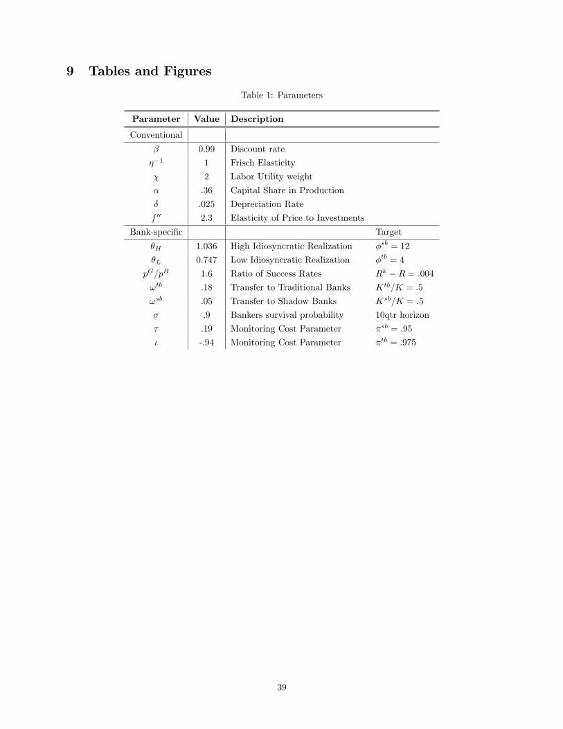
9 Tables and Figures

Table 1: Parameters

Parameter Value Description

Conventional

� 0.99 Discount rate

��1 1 Frisch Elasticity

� 2 Labor Utility weight

� .36 Capital Share in Production

� .025 Depreciation Rate

f 00 2.3 Elasticity of Price to Investments

Bank-speci�c Target

�H 1.036 High Idiosyncratic Realization �sb = 12

�L 0.747 Low Idiosyncratic Realization �tb = 4

pG=pB 1.6 Ratio of Success Rates Rk �R = :004

!tb .18 Transfer to Traditional Banks Ktb=K = :5

!sb .05 Transfer to Shadow Banks Ksb=K = :5

� .9 Bankers survival probability 10qtr horizon

� .19 Monitoring Cost Parameter �sb = :95

� -.94 Monitoring Cost Parameter �tb = :975

39

Table 2: Steady State Values

Steady State Values

Baseline Model Traditional Banking Economy Frictionless Economy

Q 1 1 1

Y 2.2390 2.0706 2.3234

Ch 1.7264 1.6659 1.7822

K 20.5062 17.1137 22.5962

�̂ 1 1.0014 1.0011

Ktb=K .5 1

Ksb=K .5

�tb 4 4.0502

�sb 12

�tb .975 0.9771

�sb .97

�̂ .9625 0.9771 0.9738

Rk �R .004 .008 .002

40

Figure 3: TFP shock, 1% drop in At, persistence .95

0 20 40-1

-0.8

-0.6

-0.4

-0.2

0

A

%∆ from ss

0 20 40-2

-1.5

-1

-0.5

0

Y

Baseline TBE FE

0 20 40-1.5

-1

-0.5

0

C

0 20 40-2

-1.5

-1

-0.5

0

K

%∆ from ss

0 20 40-3

-2

-1

0

1

Q

0 20 40-0.4

-0.3

-0.2

-0.1

0

0.1Θ̂

0 20 40-12

-10

-8

-6

-4

-2

0

Ksb

%∆ from ss

0 20 40-30

-25

-20

-15

-10

-5

0

Nsb

0 20 40-8

-6

-4

-2

0

2

πsb

0 20 40-2

0

2

4

6

8

Ktb

%∆ from ss

0 20 40-4

-2

0

2

4

6

8

Ntb

0 20 40-0.1

0

0.1

0.2

0.3

0.4

πtb

41

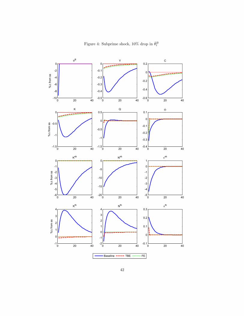
Figure 4: Subprime shock, 10% drop in θ̄Bt

0 20 40-10

-8

-6

-4

-2

0

θB

%∆ from ss

0 20 40-0.5

-0.4

-0.3

-0.2

-0.1

0

Y

Baseline TBE FE

0 20 40-0.6

-0.4

-0.2

0

0.2

C

0 20 40-1.5

-1

-0.5

0

K

%∆ from ss

0 20 40-1.5

-1

-0.5

0

0.5

Q

0 20 40-0.4

-0.3

-0.2

-0.1

0

0.1Θ̂

0 20 40-6

-5

-4

-3

-2

-1

0

Ksb

%∆ from ss

0 20 40-20

-15

-10

-5

0

Nsb

0 20 40-5

-4

-3

-2

-1

0

1

πsb

0 20 40-1

0

1

2

3

4

Ktb

%∆ from ss

0 20 40-2

-1

0

1

2

3

4

Ntb

0 20 40-0.1

0

0.1

0.2

0.3

πtb

42

Figure 5: Cross-sectional standard deviation of equity returns

0 10 20 30 40-10

0

10

20

30

40

50

60

70

%∆ from ss

Cross-sectional stdev Tfp-shock

0 10 20 30 40-5

0

5

10

15

20

25

30

35

40

%∆ from ss

Cross-sectional stdev Subprime-shock

std-dev SB std-dev TB std-dev Financial Sector

43

Figure 6: Screening cost shock, 5% increase in τt, peristence .5

0 20 400

1

2

3

4

5

6

τ

%∆ from ss

0 20 40-0.3

-0.2

-0.1

0

0.1

Y

Baseline TBE FE

0 20 40-0.6

-0.4

-0.2

0

0.2

C

0 20 40-1

-0.5

0

0.5

K

%∆ from ss

0 20 40-0.4

-0.2

0

0.2

0.4

Q

0 20 40-0.3

-0.2

-0.1

0

0.1Θ̂

0 20 40-3

-2.5

-2

-1.5

-1

-0.5

0

Ksb

%∆ from ss

0 20 40-8

-6

-4

-2

0

Nsb

0 20 40-4

-3

-2

-1

0

1

πsb

0 20 40-0.5

0

0.5

1

1.5

Ktb

%∆ from ss

0 20 40-1.5

-1

-0.5

0

0.5

1

1.5

Ntb

0 20 40-3

-2

-1

0

1

πtb

44

Figure 7: One time transfer from SB to TB equal to 1% of SB net worth

0 20 40-0.06

-0.05

-0.04

-0.03

-0.02

-0.01

0

Y

%∆ from ss

0 20 40-0.08

-0.06

-0.04

-0.02

0

0.02

0.04

C

0 20 40-0.3

-0.2

-0.1

0

0.1

I

0 20 40-0.2

-0.15

-0.1

-0.05

0

K

%∆ from ss

0 20 40-0.2

-0.15

-0.1

-0.05

0

0.05

Q

0 20 40-0.03

-0.02

-0.01

0

0.01Θ̂

0 20 40-1.5

-1

-0.5

0

Ksb

%∆ from ss

0 20 40-3

-2.5

-2

-1.5

-1

-0.5

0

Nsb

0 20 40-0.8

-0.6

-0.4

-0.2

0

0.2

πsb

0 20 400

0.2

0.4

0.6

0.8

1

Ktb

%∆ from ss

0 20 400

0.2

0.4

0.6

0.8

1

Ntb

0 20 40-0.01

0

0.01

0.02

0.03

0.04

πtb

45

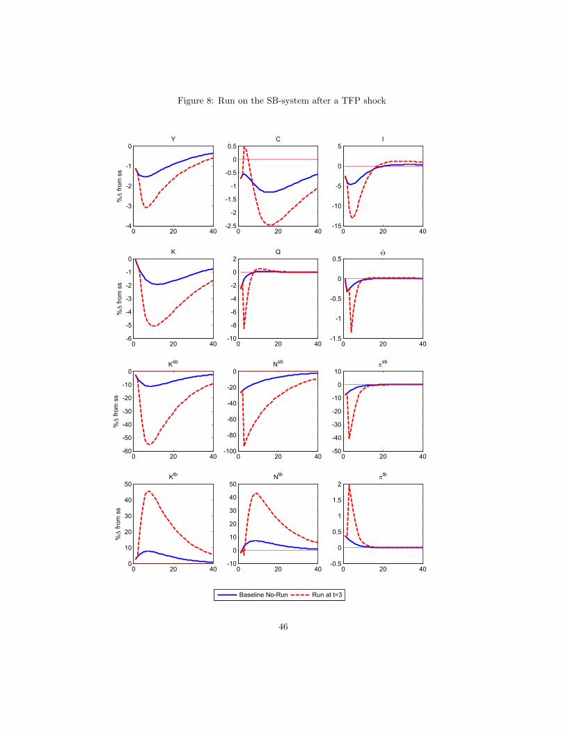
Figure 8: Run on the SB-system after a TFP shock

0 20 40-4

-3

-2

-1

0

Y

%∆ from ss

Baseline No-Run Run at t=3

0 20 40-2.5

-2

-1.5

-1

-0.5

0

0.5

C

0 20 40-15

-10

-5

0

5

I

0 20 40-6

-5

-4

-3

-2

-1

0

K

%∆ from ss

0 20 40-10

-8

-6

-4

-2

0

2

Q

0 20 40-1.5

-1

-0.5

0

0.5Θ̂

0 20 40-60

-50

-40

-30

-20

-10

0

Ksb

%∆ from ss

0 20 40-100

-80

-60

-40

-20

0

Nsb

0 20 40-50

-40

-30

-20

-10

0

10

πsb

0 20 400

10

20

30

40

50

Ktb

%∆ from ss

0 20 40-10

0

10

20

30

40

50

Ntb

0 20 40-0.5

0

0.5

1

1.5

2

πtb

46

Figure 9: Run on the SB-system after a subprime shock

0 20 40-2.5

-2

-1.5

-1

-0.5

0

Y

%∆ from ss

Baseline No-Run Run at t=3

0 20 40-3

-2

-1

0

1

2

C

0 20 40-15

-10

-5

0

5

I

0 20 40-5

-4

-3

-2

-1

0

K

%∆ from ss

0 20 40-10

-8

-6

-4

-2

0

2

Q

0 20 40-1.5

-1

-0.5

0

0.5Θ̂

0 20 40-60

-50

-40

-30

-20

-10

0

Ksb

%∆ from ss

0 20 40-100

-80

-60

-40

-20

0

Nsb

0 20 40-50

-40

-30

-20

-10

0

10

πsb

0 20 400

10

20

30

40

50

Ktb

%∆ from ss

0 20 40-10

0

10

20

30

40

50

Ntb

0 20 40-0.5

0

0.5

1

1.5

2

πtb

47

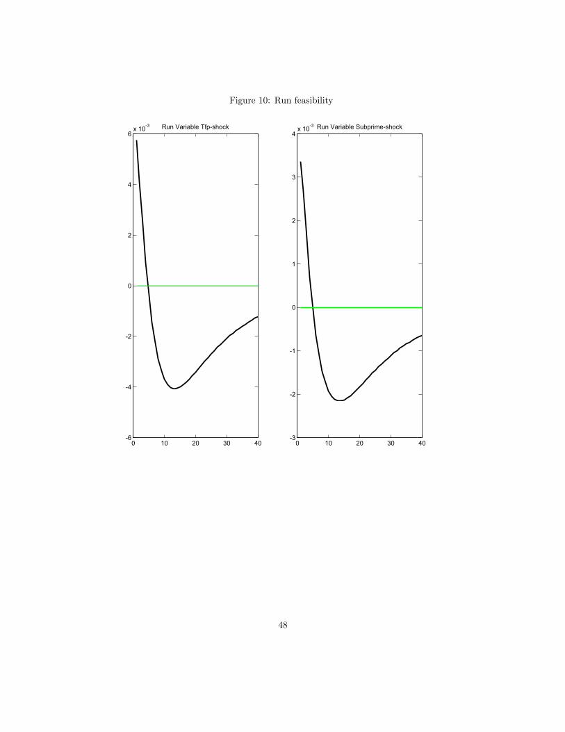
Figure 10: Run feasibility

0 10 20 30 40-6

-4

-2

0

2

4

6x 10

-3 Run Variable Tfp-shock

0 10 20 30 40-3

-2

-1

0

1

2

3

4x 10

-3 Run Variable Subprime-shock

48

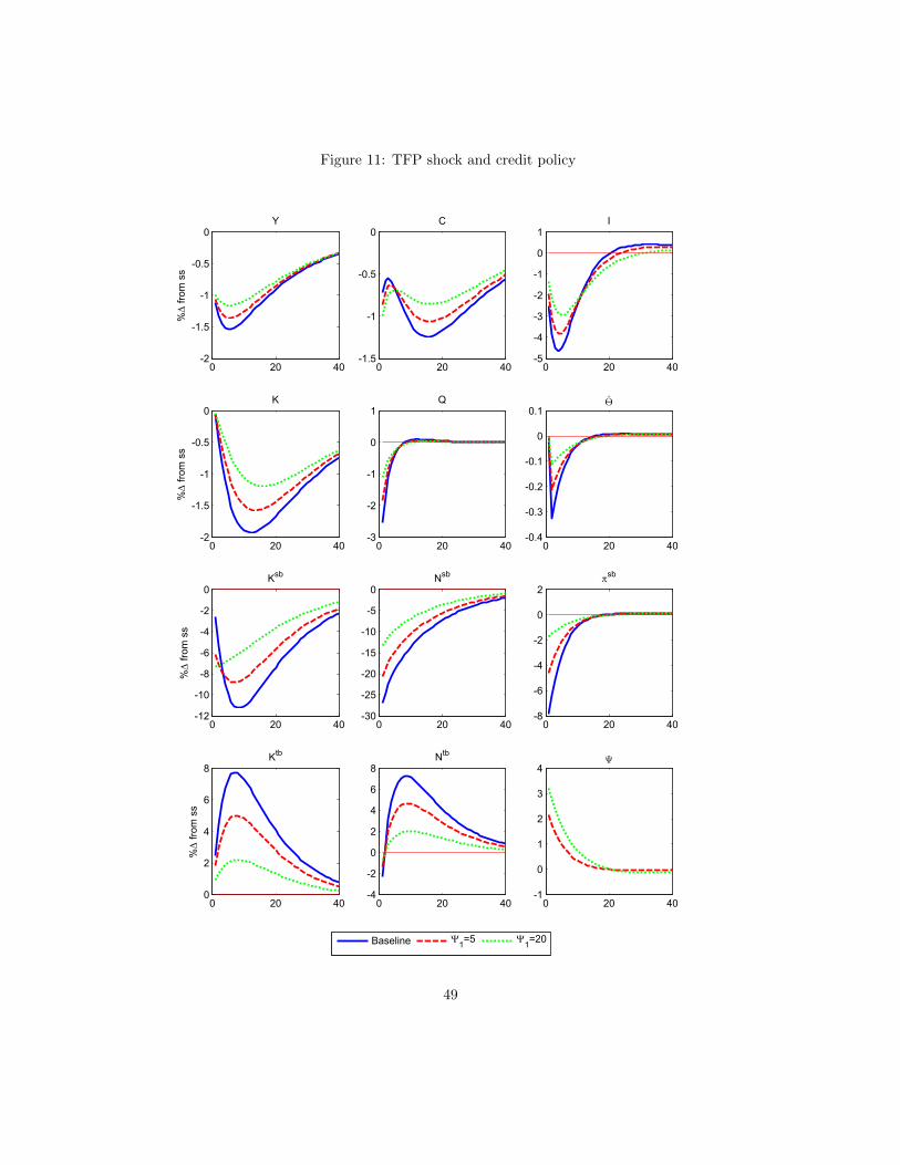
Figure 11: TFP shock and credit policy

0 20 40-2

-1.5

-1

-0.5

0

Y

%∆

fro

m s

s

Baseline Ψ1=5 Ψ

1=20

0 20 40-1.5

-1

-0.5

0

C

0 20 40-5

-4

-3

-2

-1

0

1

I

0 20 40-2

-1.5

-1

-0.5

0

K

%∆

fro

m s

s

0 20 40-3

-2

-1

0

1

Q

0 20 40-0.4

-0.3

-0.2

-0.1

0

0.1Θ̂

0 20 40-12

-10

-8

-6

-4

-2

0

Ksb

%∆

fro

m s

s

0 20 40-30

-25

-20

-15

-10

-5

0

Nsb

0 20 40-8

-6

-4

-2

0

2

πsb

0 20 400

2

4

6

8

Ktb

%∆

fro

m s

s

0 20 40-4

-2

0

2

4

6

8

Ntb

0 20 40-1

0

1

2

3

4Ψ

49

Figure 12: Subprime shock and credit policy

0 20 40-0.5

-0.4

-0.3

-0.2

-0.1

0

Y

%∆ from ss

Baseline Ψ1=5 Ψ

1=20

0 20 40-0.6

-0.4

-0.2

0

0.2

C

0 20 40-1.5

-1

-0.5

0

0.5

1

I

0 20 40-1.5

-1

-0.5

0

K

%∆ from ss

0 20 40-1.5

-1

-0.5

0

0.5

Q

0 20 40-0.4

-0.3

-0.2

-0.1

0

0.1Θ̂

0 20 40-6

-5

-4

-3

-2

-1

0

Ksb

%∆ from ss

0 20 40-20

-15

-10

-5

0

Nsb

0 20 40-5

-4

-3

-2

-1

0

1

πsb

0 20 40-1

0

1

2

3

4

Ktb

%∆ from ss

0 20 40-2

-1

0

1

2

3

4

Ntb

0 20 40-0.5

0

0.5

1

1.5

2

2.5Ψ

50

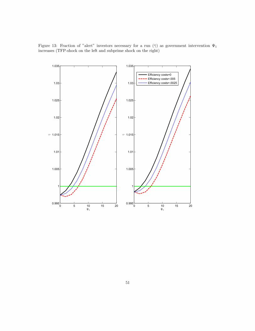
Figure 13: Fraction of ”alert” investors necessary for a run (γ̄) as government intervention Ψ1

increases (TFP-shock on the left and subprime shock on the right)

0 5 10 15 200.995

1

1.005

1.01

1.015

1.02

1.025

1.03

1.035

γ̄

Ψ1

0 5 10 15 200.995

1

1.005

1.01

1.015

1.02

1.025

1.03

1.035

γ̄

Ψ1

Efficiency costs=0

Efficiency costs=.005

Efficiency costs=.0025

51