MPRAMunich Personal RePEc Archive

A Model of Competition in the SolarPanel Industry

Unni Pillai and Jamison McLaughlin

University at Albany, SUNY, University of Michigan

May 2013

Online at http://mpra.ub.uni-muenchen.de/46655/MPRA Paper No. 46655, posted 2. May 2013 17:33 UTC

A Model of Competition in the Solar Panel Industry ✩

Unni Pillai∗, Jamison McLaughlin

College of Nanoscale Science and Engineering

University at Albany - SUNY, Albany, NY, USA.

Abstract

We develop a model of competition in the solar panel industry. Solar firms manufacture pan-

els that are differentiated both vertically and horizontally, and compete by setting quantities.

The equilibrium of the model is consistent with a set of stylized facts that we document,

including variation in prices, markups and market shares across firms. We calibrate the

model using a new dataset data on prices, costs and shipments of leading solar companies,

as well as solar sales in four leading markets. The calibrated model is applied to evaluate the

impact of a decline in the price of polysilicon, a key raw material used in the manufacture

of solar panels, on the equilibrium price of solar panels.

Keywords: Photovoltaics, Competition, Polysilicon

JEL: L19, L13, O30

1. Introduction

The electricity generation sector is the leading contributor of greenhouse gas emissions.

Most plans to stabilize greenhouse gas emissions view solar photovoltaics as an electricity

generation technology with potential to replace a sizeable section of fossil fuel generation

(see Nakicenovic and Riahi (2002); Baker and Solak (2011); Lewis and Nocera (2006)). At

∗Corresponding author. College of Nanoscale Science and Engineering, University at Albany - SUNY,257-Fuller Road, Albany, NY-12203, USA. Email :usadasivanpillai@albany.edu

Preprint submitted to Energy Economics March 4, 2013

present however, electricity from solar photovoltaics constitute a very small fraction of the

world electricity production. The cost of generating electricity from solar PV systems have

fallen over time. A major factor behind this decline has been the continual decrease in the

price of solar panels (also called solar modules), the principal component in PV systems.

These declines have brought the price of solar generated electricity closer to the price of

electricity generated from conventional sources, but a gap still remains.

There has been an extensive examination in the literature of factors that have contributed

to the decline in solar module prices. Most of the existing studies are based on learning

curves, which extrapolate past observations about the relationship between the price of

solar modules and the volume of production (for example, see Swanson (2006) and Schaeffer

(2004)). There have been other studies, for example Nemet (2006) and Bruton (2002),

which look at the contribution of various factors like plant size and module efficiency in

reducing the price of solar modules. Learning curve models and models like Nemet (2006)

are suited to explain how different factors affect the cost of production. The use of these

models in predicting changes in price depend entirely on the assumption that changes in

cost will translate into identical changes in price. If the solar module industry was perfectly

competitive with modules being sold at a price equal to its marginal cost, then any reduction

in cost would result in the same reduction in price. The solar module industry, however,

is not a perfectly competitive industry. As documented in section 2, there are differences

in prices, markups and market shares of different firms in the industry, all indicative of

deviation from the assumption of perfect competition. Under imperfect competition, the

effect on price of a change in cost would depend on how firms respond to the change in cost.

The use of price instead of cost in learning curve models and in Nemet (2006) provide a useful

simplification, but ignoring the role of competition among firms in determining equilibrium

prices is not without consequence. For example, Nemet (2006) finds that changes in factors

that affect cost can only explain a part of the change in the price of solar modules in some

of the years considered in his study. He argues that there was an increase in the extent of

2

competition in the industry in those years, which might partially account for the residual

variation in price over and above the variation in cost. A contribution of this paper is to

develop a model that explicitly incorporates competition among firms in the industry and

can be used to evaluate how changes in costs affect the selling price of solar modules.

In section 2 we lay down three empirical observations that capture the salient features of

competition in the industry. In section 3, we develop a model that is consistent with these

observations. The model derives a demand function for solar modules, taking into account

the behavior of electric utility companies, power producers and solar module manufacturers.

Electric utility companies, who deliver electricity to consumers (either directly or through

local distribution companies), purchase electricity from solar power producers, who can be

individual households, businesses or commercial power producing companies. These solar

power producers in turn demand solar modules from module manufacturers. The solar

modules made by different firms are differentiated both vertically and horizontally. The

module firms compete by setting quantities and we derive a set of equations that can be

used to compute the equilibrium prices, markups and market shares in this Cournot model.

The model can be extended to incorporate other features of the solar industry, and sec-

tion 4 describes some of the possible extensions. The inclusion of non-module (or balance-

of-system) costs does not affect the equilibrium strategies of the module firms but increases

the price of solar generated electricity. The effect of differences in insolation (the intensity

of incident sunlight) can be easily incorporated in the model. Finally, the model can be

extended to consider the impact of changes in usage of different factors of production on

price of solar modules. These extensions can be used to investigate the impact of decline

in balance-of-system costs, the impact of differences in insolation, and the impact of tech-

nological improvements like reduction in raw material requirements or plant automation on

the equilibrium price of solar modules and of electricity generated from solar modules. The

data necessary to calibrate the basic model described in section 3 can obtained from publicly

available sources, as described in section 5.

3

In section 6, we put the calibrated model to use for one application. The price of polysili-

con, a key raw material used in the manufacture of solar modules, has declined in the last few

years and analysts expect further reductions in the price of polysilicon. We use the model to

evaluate the impact of decline in polysilicon price on the price of solar modules. Alternative

simulations are performed to evaluate the impact of decline in polysilicon price if competition

among firms intensify because of standardization of modules, or if solar generated electricity

becomes more differentiated from electricity generated from other sources.

We begin by giving a brief description of the solar module industry in the next section.

2. The Solar Module Industry

The solar module industry consists of a number of firms located in many countries. The

output of the firms is usually measured in watts of solar modules.1 In 2011, the solar mod-

ule industry shipped around 28,000 megawatts of solar modules.2 Contrary to the casual

observation that solar modules are standardized homogenous products, solar modules sold

by different companies differ in many ways. The most significant of these differences is in

the efficiency with which they convert sunlight to electricity. The more efficient the solar

modules are, the smaller is the size of the module required to produce a unit of electricity.

Small module size (or fewer modules) translate to lower expenses on the accessories required

to mount the module on a rooftop or ground. Thus higher efficiency is valued in a quan-

tifiable way, and we capture this by treating solar modules as being vertically differentiated

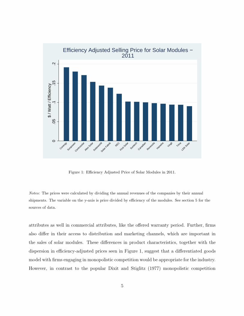
with regard to efficiency. Even after adjusting for the efficiency of the modules, there is a

dispersion in the price charged per watt by different firms in the industry (see Figure 1).

In addition to efficiency, the modules sold by different companies differ in other technical

1Ideally, a solar module rated at 1 watt when exposed to sunlight for 1 hour would generate 1 watt-hour

of electricity. In practice however, the amount of electricity generated depends on the intensity of sunlight,

the angle at which the modules are mounted, etc.2A megawatt is a million watts.

4

0.0

5.1

.15

.2$

/ Wat

t / E

ffici

ency

LDK S

olar

Trina

Yingli

Hanwha

Renes

ola

Canad

ian

Sunte

ch

First S

olar

REC

Solar F

abrik

Solarw

orld

Aleo S

olar

Centro

solar

Sunpo

wer

Coner

gy

Efficiency Adjusted Selling Price for Solar Modules −2011

Figure 1: Efficiency Adjusted Price of Solar Modules in 2011.

Notes: The prices were calculated by dividing the annual revenues of the companies by their annual

shipments. The variable on the y-axis is price divided by efficiency of the modules. See section 5 for the

sources of data.

attributes as well in commercial attributes, like the offered warranty period. Further, firms

also differ in their access to distribution and marketing channels, which are important in

the sales of solar modules. These differences in product characteristics, together with the

dispersion in efficiency-adjusted prices seen in Figure 1, suggest that a differentiated goods

model with firms engaging in monopolistic competition would be appropriate for the industry.

However, in contrast to the popular Dixit and Stiglitz (1977) monopolistic competition

5

model, there is also a dispersion in the markups charged by the firms in the industry. Figure

2 plots the markups (gross margins) of companies against their market shares. As can be seen

from the figure, bigger firms tend to have bigger markups as would be implied by a Cournot

model, although there are deviations from a simple linear relationship. The observations

above can be summarized in three stylized facts,

1. There is a dispersion in efficiency adjusted prices across firms.

2. There is a dispersion in markups across firms.

3. Larger firms tend to have bigger markups.

The next section develops a model of the solar module industry that is consistent with

the three observations above.

3. The Model

Our model is a modification of the model developed in Smith and Venables (1988) and

Atkeson and Burstein (2008). We develop the model in a number of steps, and begin by

deriving the demand for solar modules in the next section.

3.1. Demand

The electricity industry consists of three vertically connected segments. At the very top

are the electric utility companies who sell electricity to final consumers. At the next rung are

the power producers (including solar power producers) who own power plants and generate

electricity which they sell to the electric utility companies. At the bottom rung are the

equipment companies, like solar module companies, who manufacture the equipment used

by power producers to generate electricity. Demand for solar electricity, and hence solar

modules, is essentially driven by government policies, which differ across countries. In many

European countries (Germany, Italy, Spain, France and Czechoslovakia), the government

requires electric utility companies to buy electricity generated by solar power producers at a

6

010

2030

40M

arku

p (%

)

0 2 4 6 8Market Share (%)

Module Markups and Revenue Market Shares −2011

Figure 2: Bigger firms tend to have higher markups.

Notes: Each point in the graph corresponds to a firm. The market shares were obtained by dividing the

annual revenue of the firm by an estimate of the total sales of solar modules. The estimate of total sales

was obtained by multiplying the average price of firms in the dataset by the total shipment of solar

modules in 2011.

guaranteed price. In many U.S states on the other hand, the demand for solar modules stem

from Renewable Portfolio Standard (RPS) mandates, which require electric utility companies

to obtain a portion of the total electricity that they sell from renewable sources. We abstract

from the differences in policies and assume that for an electric utility company, the effect

of these policies is to make solar generated electricity an imperfect substitute for electricity

7

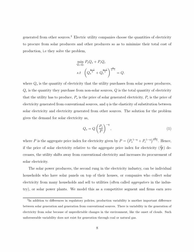
generated from other sources.3 Electric utility companies choose the quantities of electricity

to procure from solar producers and other producers so as to minimize their total cost of

production, i.e they solve the problem,

minQs,Qc

PsQs + PcQc

s.t

(

Qη−1

ηs + Q

η−1

ηc

)η

η−1

= Q.

where Qs is the quantity of electricity that the utility purchases from solar power producers,

Qc is the quantity they purchase from non-solar sources, Q is the total quantity of electricity

that the utility has to produce, Ps is the price of solar generated electricity, Pc is the price of

electricity generated from conventional sources, and η is the elasticity of substitution between

solar electricity and electricity generated from other sources. The solution for the problem

gives the demand for solar electricity as,

Qs = Q

(

Ps

P

)

−η

, (1)

where P is the aggregate price index for electricity given by P =(

Ps1−η + Pc

1−η)

1

1−η . Hence,

if the price of solar electricity relative to the aggregate price index for electricity (Ps

P) de-

creases, the utility shifts away from conventional electricity and increases its procurement of

solar electricity.

The solar power producers, the second rung in the electricity industry, can be individual

households who have solar panels on top of their houses, or companies who collect solar

electricity from many households and sell to utilities (often called aggregators in the indus-

try), or solar power plants. We model this as a competitive segment and firms earn zero

3In addition to differences in regulatory policies, production variability is another important difference

between solar generation and generation from conventional sources. There is variability in the generation of

electricity from solar because of unpredictable changes in the environment, like the onset of clouds. Such

unforeseeable variability does not exist for generation through coal or natural gas.

8

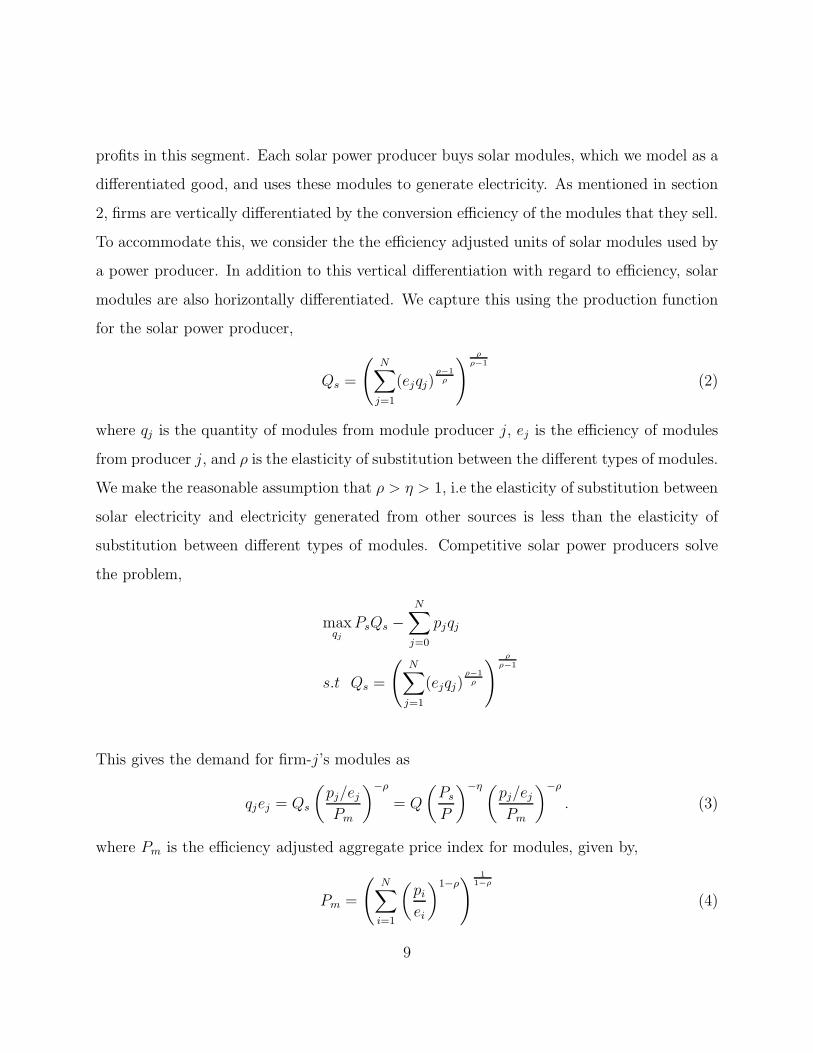
profits in this segment. Each solar power producer buys solar modules, which we model as a

differentiated good, and uses these modules to generate electricity. As mentioned in section

2, firms are vertically differentiated by the conversion efficiency of the modules that they sell.

To accommodate this, we consider the the efficiency adjusted units of solar modules used by

a power producer. In addition to this vertical differentiation with regard to efficiency, solar

modules are also horizontally differentiated. We capture this using the production function

for the solar power producer,

Qs =

(

N∑

j=1

(ejqj)ρ−1

ρ

)

ρ

ρ−1

(2)

where qj is the quantity of modules from module producer j, ej is the efficiency of modules

from producer j, and ρ is the elasticity of substitution between the different types of modules.

We make the reasonable assumption that ρ > η > 1, i.e the elasticity of substitution between

solar electricity and electricity generated from other sources is less than the elasticity of

substitution between different types of modules. Competitive solar power producers solve

the problem,

maxqj

PsQs −

N∑

j=0

pjqj

s.t Qs =

(

N∑

j=1

(ejqj)ρ−1

ρ

)

ρ

ρ−1

This gives the demand for firm-j’s modules as

qjej = Qs

(

pj/ejPm

)

−ρ

= Q

(

Ps

P

)

−η (pj/ejPm

)

−ρ

. (3)

where Pm is the efficiency adjusted aggregate price index for modules, given by,

Pm =

(

N∑

i=1

(

piei

)1−ρ)

1

1−ρ

(4)

9

Hence the demand for solar modules for firm-j depends both on how expensive the firm’s solar

module is relative to that sold by other firms,

(

pj/ejPm

)

, and how expensive solar electricity

is relative to electricity from other generation sources

(

Ps

P

)

. Since solar power producers

are perfectly competitive, they make zero profit, and hence the price of solar electricity is

given by,

Ps = Pm (5)

Hence the demand equation (3) can be written as

qjej = Q

(

Ps

P

)

−η (pj/ejPs

)

−ρ

. (6)

Having derived the demand facing each module producer, we move on to the optimal

pricing decisions made by the module producers given the demand function above that they

face.

3.2. Equilibrium

We assume that the solar module firms engage in Cournot competition. Each solar firm

takes P , the price index for electricity as given when making its quantity and price decisions.

But the firm considers the effect of its decisions on the solar module price index, Pm, and

the price of solar electricity, Ps. We assume that module firms have a constant marginal cost

of production, and denote module firm-j’s marginal cost by cj4. Firm-j solves the problem,

maxqj

pjqj − cjqj

s.t qjej = Q

(

Ps

P

)

−η (pj/ejPs

)

−ρ

,

Ps =

(

N∑

i=1

(pi/ei)1−ρ

)

1

1−ρ

4It is possible that the marginal cost would decrease with increases in production (see Nemet (2006)),

but we ignore that for purposes of tractability.

10

Solving the above problem gives the result that equilibrium price exceeds cost by a factor

given by,pjcj

=1

1 −sjη−

1 − sjρ

, (7)

where sj =pjqj∑

i piqiis the market share of firm-j. Equation (7) can be rewritten to obtain

the markup (gross margin) as,

pj − cjpj

=sjη

+1 − sj

ρ(8)

Further, using equation (3), the market share can be written as

sj =pjqjN∑

i=1

piqi

=pj

1ejQs

(

pj/ejPs

)

−ρ

N∑

i=1

pi1eiQs

(

pi/eiPs

)

−ρ=

(pj/ej)1−ρ

N∑

i=1

(pi/ei)1−ρ

(9)

The model is consistent with the observations about competition in the industry summa-

rized in Section 2. Since ρ > 1, equation (9) implies that bigger firms (larger market share

sj) charge a lower efficiency-adjusted price (p/e). Given this, and the assumption that ρ > η,

equation (7) implies that firms with higher efficiency-adjusted marginal cost (c/e) charge a

higher efficiency adjusted-price (p/e).5 Thus firms charge different efficiency-adjusted prices,

consistent with Figure 1 and stylized fact 1. Equation (8) implies that firms charge different

markups, consistent with stylized fact 2. Since ρ > η, equation (8) also implies that bigger

firms charging higher markups, consistent with Figure 2 and stylized fact 3.

5This is most easily seen by considering equation (7) for two firms, say firm 1 and firm 2. Equation (7)

implies that

p1/e1p2/e2

ρ−1

ρ− s1

(

1

ρ− 1

η

)

ρ−1

ρ− s2

(

1

ρ− 1

η

) =c1/e1c2/e2

.

Hence if c1/e1 > c2/e2, it must be that p1/e1 > p2/e2. If p1/e1 < p2/e2, then equation (9) implies that

s1 > s2, and hence the left hand side of equation above will be less than one and right hand side greater

than one.

11

Equation (7) makes clear that price can vary from cost. The factor by which price is

greater than cost depends on the market share of the firm, and the elasticities η and ρ.

For bigger firms, the price/cost factor is larger. As η increases, price/cost factor decreases

because the differentiation between solar generated electricity and electricity from other

sources decreases, and they become more direct competitors. As ρ increases, the price/cost

factor decreases because the differentiation among the different module firms decreases and

they become more direct competitors.

It is straightforward to compute the equilibrium of the model, if the unit costs {cj},

efficiencies {ej}, and elasticities η and ρ are known. Substituting equation (9) in equation

(8) gives a system N non-linear equations in N unknowns prices, and hence can be solved to

obtain the equilibrium prices {pj}. The above model provides a tool to evaluate how module

prices change in response to changes in the cost of production of modules. In many cases

one is interested not only in the price of modules, but also in the price of a fully installed

solar generation system, as well as in the price of the electricity generated from such systems.

In section 4 we outline how the above model can be extended to accommodate this. With

additional data one can use the extension of the model to evaluate the impact of cost changes

on the price of a fully installed solar system and on the price of solar generated electricity.

4. Extensions of the Model

The basic model of competition in the solar panel industry described in section 3 can be

extended to incorporate other features of the industry.

4.1. Balance of System Costs and Insolation

The solar modules considered in the model above form the core of a solar photovoltaic

electricity generation system. In addition to the cost of the module itself, the cost of a

solar generation system also includes the cost of electrical components necessary to connect

the system with the electrical grid and the cost of mounting structures necessary to fix the

12

modules on a rooftop or on the ground. There are also non-hardware “soft-costs” - the cost

of getting a permit to install the system, the cost of labor necessary to install the system,

etc. As module costs are declining, the other costs, which are often collectively labeled the

balance-of-system costs, are becoming an important fraction of the total cost of the system

(see Feldman et al. (2012) and Aboudi (2012)). The balance-of-system costs can be added

to the model in a simple manner, by assuming that cost of the total solar system is a factor

k times the module cost, i.e the total cost is now kN∑

i=1

pjqj .

Further, in addition to the characteristics of the solar module, the amount of electricity

that can be generated from a solar module also depends on the amount of sunlight that is

incident on the module. This parameter is referred to in the industry as insolation. This can

be incorporated into the model by modifying the production function in equation (2) to,

Qs = h

(

N∑

j=1

(ejqj)ρ−1

ρ

)

ρ

ρ−1

(10)

where the insolation factor h converts the rated power into the actual amount of electricity

produced.

It is to be noted that the balance-of-system cost factor k and insolation h can vary

across markets. The balance-of-system costs depend on the labor cost, permitting policies

in place and so on. For example, Seel et al. (2012) report that the balance-of-system cost

in Germany was lower than in the U.S in 2010. Similarly, the insolation factor would also

vary across markets, with sunny countries like Spain or India having higher h than countries

like Denmark or Germany. One could apply the above model to a specific region where the

insolation and balance-of-system cost factor remains the same across different solar power

producers, under the assumption that each module producer treats every region as a different

market. Under this assumption, the problem of the solar power producer in market-i becomes

maxqj

PsQs − kiN∑

j=0

pjqj

13

s.t Qs = hi

(

N∑

j=1

(ejqj)ρ−1

ρ

)

ρ

ρ−1

The demand function for each module and the price index for modules remain the same

as in the basic model (as given in equations (3) and (4) respectively). The equilibrium prices

and markups also remain the same as before, as given in equations (7) and (8) respectively.

But the price of solar generated electricity becomes P is =

ki

hiPm. Thus the price of solar

generated electricity will be lower in regions with lower balance of system costs and higher

insolation. With data on ki and hi, one could use this extension of the basic model to

evaluate the impact of a decrease in balance-of-system costs on the price of solar generated

electricity.

4.2. Technological Improvements

Many technological improvements have contributed to the decline in module prices. Im-

provements in efficiency has been an important contributor to the decline in module prices,

and the model described in section 3 can be used to simulate the impact of increases in

efficiency on module prices. Another important facet of technological progress has been in

the reduction of the quantity of inputs needed to produce a watt of modules. The quantity

of polysilicon needed to produce 1 watt of solar modules has decreased over the years (see

Swanson (2006) and Nemet (2006)). Such technological improvements can be incorporated

into the model by considering a Leontief production function for the production of solar

modules,

qj = Min(aMj , bLj)

where Mj is quantity of polysilicon used, Lj is the amount of labor used, a is the unit polysil-

icon requirement and b is the unit labor requirement. Module firm-j’s profit maximization

14

problem now becomes,

maxMj ,Lj

pjqj − wLj − vMj

s.t qj = Min(aMj , bLj),

s.t qjej = Q

(

Ps

P

)

−η (pj/ejPs

)

−ρ

,

Ps =

(

N∑

i=1

(pi/ei)1−ρ

)

1

1−ρ

where v is the price of polysilicon and w is the labor wage rate. The solution to the problem

remains the same as the ones described in section 3, with cj being replaced byw

b+

v

a. The

model can then be simulated to understand the impact of a decrease in unit polysilicon

requirement (a decrease in a), or the effect of a decrease in price of polysilicon (a decrease

in v).

In section 6, we describe how we can calibrate the model and simulate it to calculate

the impact of a decrease in v, the price of polysilicon. In the next section we describe the

sources of the data that we use to estimate the model parameters necessary to calibrate the

model.

5. Data and Calibration

In the simulations to evaluate the impact of a decline in polysilicon price on module price,

we model the solar module industry as being comprised of 15 companies. These include the

companies which were in the top 10 in terms of shipments in 2011 (Suntech, First Solar,

Yingli, Trina, Canadian Solar, Sharp, Hanwha Solarone, Jinko, Solarworld and LDK Solar)

and 5 other leading module manufacturers (Sunpower, REC, JA Solar, Kyocera and Aleo

Solar). Together these companies accounted for over 60% of the global shipments in solar

modules in 2011, and companies not in the list contributed less than 2 % each to the total

industry shipments. Among the 15 companies, 14 companies make solar modules using

polysilicon as the raw material. However the lowest cost firm, First Solar, uses a technology

15

different from the rest, and does not use polysilicon in its production process.6 We leave the

cost of First Solar at its 2011 level in our simulation.

The variable production costs of 12 of the above companies were obtained from their

annual reports. For each company, annual data was collected on cost of goods sold (COGS),

revenues and shipments. For the U.S companies, the data was collected from their annual

10-K statements. All the companies in the dataset that are based in China are registered

in U.S stock exchanges, and hence file an annual 20-F statement with the U.S Securities

and Exchange Commission. The format for the 20-F statement is similar to 10-K statement,

providing comparability between the data used for companies based in U.S and China. The

cost of goods sold (COGS) for the companies in the dataset filing 10-K and 20-F includes

the cost of materials, direct labor cost, utilities and depreciation of capital, and excludes the

expenses on R&D, marketing and general administration. Hence the COGS reported by these

companies are a good measure of their variable cost of production. For the companies based

in Europe, the data was obtained from their annual reports. While some of the European

companies report the cost of goods sold, some report only the earnings before interest and

taxes (EBIT). Subtracting the sum of EBIT and reported expenses on R&D, marketing and

general administration from the annual revenues, gives a measure of the variable cost of

production that is comparable to the COGS reported by companies registered on U.S stock

exchanges. All companies report their annual shipment of solar panels in watts.

The use of cost data derived from annual reports of companies has sometimes been

criticized in the literature. But there are a number of reasons to believe that concerns raised

are less severe for the cost data that is used in this study. First, all the companies whose

cost data is used in the analysis are pure solar companies, so the variable costs they report

in annual statements are those associated with solar production alone. Second, many of the

companies state in their annual reports that a substantial fraction of the COGS that they

6First Solar produces solar modules using Cadmium Telluride.

16

report are material costs, which are usually correctly reflected in annual reports. Third,

the unit cost of production is the most closely watched metric in the industry, and market

analysts routinely publish estimates of the units costs of companies using their own methods.

It is quite likely that the close scrutiny by industry observers puts a heavy burden on the

firms to report their costs truthfully.

The average variable cost of producing solar panels for each firm was obtained by dividing

COGS by annual shipments. For the 3 companies for whom cost data was not available

(Sharp, Kyocera, and Jinko), we used equation (8) to obtain the unit costs of the companies,

given their prices and market shares. The prices for these companies were obtained from the

Photon Magazine or from their annual reports. To provide an illustration of the accuracy of

the model in backing out costs from prices, we plot in Figure 3 the costs backed out by the

model against the actual costs of the companies for which we have cost data.

We now turn to the two demand parameters whose values are needed to simulate the

model, the elasticity of substitution between solar and non-solar electricity, η, and the elas-

ticity of substitution between solar modules, ρ. A high η would imply that solar electricity

is less differentiated from electricity generated from other sources. We estimate the demand

elasticity from the data on module price and quantity sold in four markets - Germany, Italy,

Spain and France. The data on annual solar installations in these countries is taken from

IEA (2010) and is available for Germany from 1990-2010 and for the other three countries

from 1995-2010. The quantity sold in each of these markets is likely to be influenced by the

subsidy policies of the governments, which we include in the regression. We perform two

regressions to estimate η. In the first regression, we do not use any instruments for price.

In the second regression, we instrument the price of solar modules with the total market

share of firms from China in the worldwide shipments of solar modules. The entry of firms

from China prompted a decline in prices, either because of low cost of production of firms in

China or because of production subsidies offered in China. Hence the increasing penetration

of Chinese firms in the solar market represent a supply side shock not correlated to demand

17

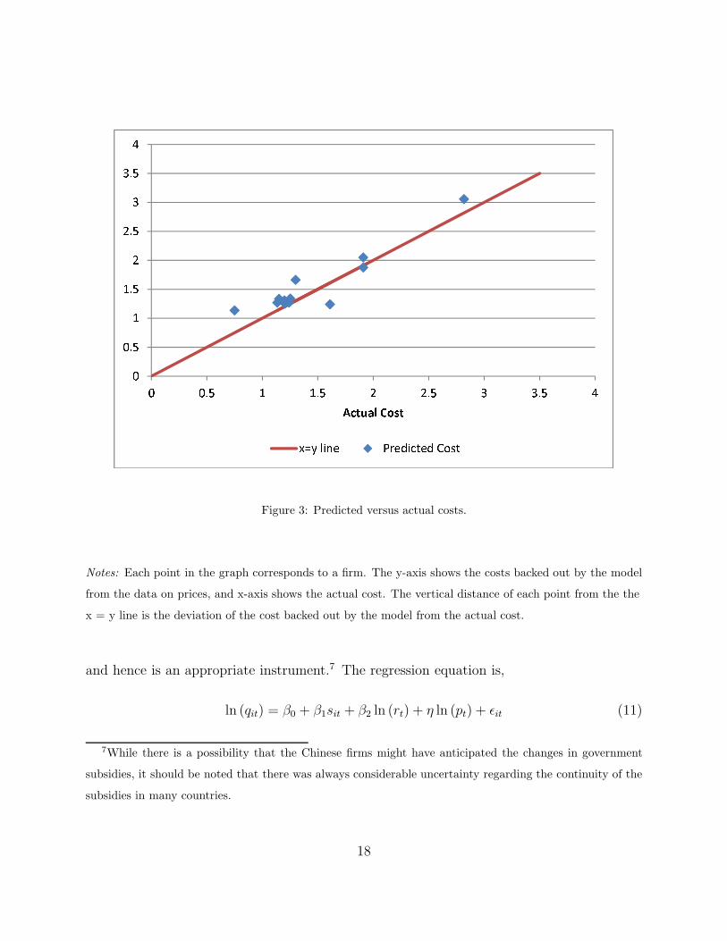
Figure 3: Predicted versus actual costs.

Notes: Each point in the graph corresponds to a firm. The y-axis shows the costs backed out by the model

from the data on prices, and x-axis shows the actual cost. The vertical distance of each point from the the

x = y line is the deviation of the cost backed out by the model from the actual cost.

and hence is an appropriate instrument.7 The regression equation is,

ln (qit) = β0 + β1sit + β2 ln (rt) + η ln (pt) + ǫit (11)

7While there is a possibility that the Chinese firms might have anticipated the changes in government

subsidies, it should be noted that there was always considerable uncertainty regarding the continuity of the

subsidies in many countries.

18

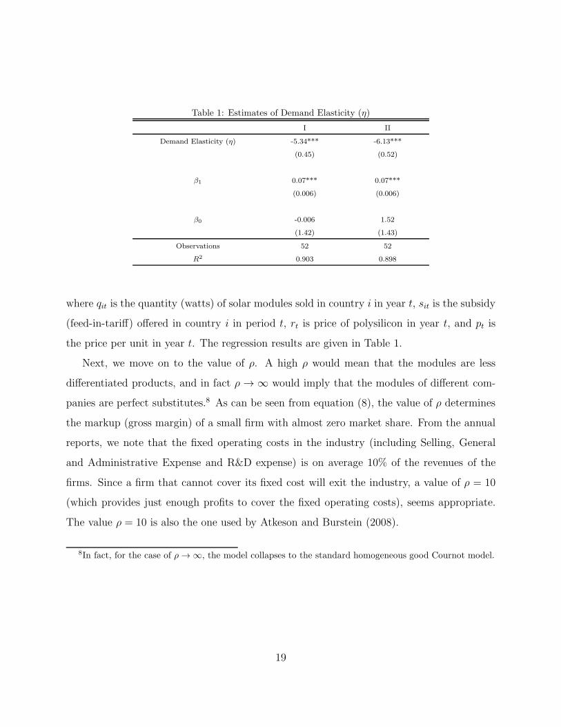
Table 1: Estimates of Demand Elasticity (η)

I II

Demand Elasticity (η) -5.34*** -6.13***

(0.45) (0.52)

β1 0.07*** 0.07***

(0.006) (0.006)

β0 -0.006 1.52

(1.42) (1.43)

Observations 52 52

R2 0.903 0.898

where qit is the quantity (watts) of solar modules sold in country i in year t, sit is the subsidy

(feed-in-tariff) offered in country i in period t, rt is price of polysilicon in year t, and pt is

the price per unit in year t. The regression results are given in Table 1.

Next, we move on to the value of ρ. A high ρ would mean that the modules are less

differentiated products, and in fact ρ → ∞ would imply that the modules of different com-

panies are perfect substitutes.8 As can be seen from equation (8), the value of ρ determines

the markup (gross margin) of a small firm with almost zero market share. From the annual

reports, we note that the fixed operating costs in the industry (including Selling, General

and Administrative Expense and R&D expense) is on average 10% of the revenues of the

firms. Since a firm that cannot cover its fixed cost will exit the industry, a value of ρ = 10

(which provides just enough profits to cover the fixed operating costs), seems appropriate.

The value ρ = 10 is also the one used by Atkeson and Burstein (2008).

8In fact, for the case of ρ → ∞, the model collapses to the standard homogeneous good Cournot model.

19

6. Impact of Polysilicon Price Decline

One of the factors that has contributed to the decline in module prices over the last few

decades is the decline in the price of polysilicon, the principal raw material used in building

crystalline silicon solar cells. The average price of solar modules has declined by a factor of

close to over 50 in the period 1975-2010, and the cost of the polysilicon needed to make one

watt of solar modules has decreased by a factor of 20 over the same period (see Figure 4).

Following a sharp increase during 2004-2008, the price of polysilicon almost halved dur-

ing 2008-2010. Yu et al. (2012) examine the reasons for the changes in polysilicon price

during 2004-2009 and conclude that demand shocks played an essential role in the fluctu-

ations, as also did changes in cost of producing polysilicon.9 Generous subsidy schemes

for solar generated electricity implemented in many European countries led to a surge in

the demand for polysilicon. The rising polysilicon prices lead to an expansion in capacity

by existing polysilicon firms and the entry of many new firms into the industry.10 Total

worldwide polysilicon capacity increased from around 50,000 metric tons in 2005 to around

300,000 metric tons in 2010 (see Prior and Campbell (2012)). Based on investment plans

announced by polysilicon suppliers, Winegarner (2011) anticipates polysilicon capacity to

increase to over 500,000 metric tons in 2015. These increases have been accompanied by

improvements in the production technology, as polysilicon firms found ways to reduce the

9Yu et al. (2012) consider oil and natural gas shocks as the main source of changes in the production cost.

In addition to demand and production cost shocks, they also find that fluctuations in exchange rates had a

significant impact on polysilicon price. Note that the price of solar modules held steady despite the spike in

polysilicon price. This was possibly because of the increasing market penetration of lower cost firms from

China during the same period.10Hemlock, the leading polysilicon supplier increased its capacity from 7700 to 36,000 metric tons from

2005 to 2010. Wacker, the second largest established polysilicon supplier, increased its capacity from 5500

to 24,000 metrics tons. New firms GCL-Poly and OCI entered the market in 2007-2008 and quickly build

their capacities to 21,000 and 27,000 metric tons in 2010.

20

.51

24

816

3264

128

256

512

$ /

Wat

t, $/

Kg

1970 1975 1980 1985 1990 1995 2000 2005 2010

Module Price Polysilicon Price

Figure 4: Decline in Solar Module Price and Cost of Polysilicon Used in Solar Modules.

Notes: The prices of solar modules for 1975-2006 were taken from Maycock (2002) and from the dataset at

Earth Policy Institute. The price of solar modules during 2007-2010 was taken as the quantity weighted

average of price of leading solar module companies. The data for polysilicon price and unit polysilicon

requirement was taken from Nemet (2006) for 1975-2002 and from Winegarner (2011) and company annual

reports for the years 2003-2010.

cost of production. The addition of new capacity and intensifying competition among new

and established polysilicon manufacturers, as well as the development of new cost reducing

innovations in the manufacture of polysilicon, have led many industry observers to forecast

a continued decline in the price of polysilicon and consequent decline in module prices (see

21

Fessler (2012) and Prior and Campbell (2012)).

We use a variation of the model described in section 4.2 to simulate the impact of the

forecasted polysilicon price drop on the price of solar modules. To focus on the impact of

polysilicon price declines, we consider a variation of the model with polysilicon as one input

and all other inputs lumped together as the second input. With the Leontief production

function described in section 4.2, this results in the unit cost of firm-j being,

cj =v

a+ zj (12)

where v is the price of polysilicon, a is the quantity of polysilicon needed to produce one

watt of solar modules, and zj is the non-polysilicon cost of firm-j. The price of polysilicon

in 2011 was constructed from annual reports of leading polysilicon companies. The annual

revenues of four polysilicon companies (Wacker, REC, GCL-Poly and Daqo) were divided

by the annual shipments to obtain the average selling price of each company. A quantity

weighted average of these prices was taken as the price of polysilicon, which was found to be

$59 per Kg. The data on a was obtained for a few of the solar module companies mentioned

in section 5 from their annual reports, and the average value obtained was 5.6 grams per watt.

The variable zj includes the costs of all other factors of production (labor, capital, utilities

and other raw materials) and was calculated from the data on cj , v and a, i.e zj = cj −v

a.

In the simulations, the values of a and zj were left at their 2011 values and the price of

polysilicon was reduced from the 2011 value of $59/Kg to $15/Kg, which is almost a 75%

reduction in the price. The simulations were done for three value of η, η = 5.5 which we

consider as a baseline case based on the estimates in section 5, a low value η = 2 and a high

value η = 10. Two values of ρ were also considered (ρ = 10, which is used in Atkeson and

Burstein (2008) and a value of ρ = 20). Note that a higher value of ρ means that products

are less differentiated, and firms have less market power. The results are shown in Table 2,

with the last column showing the quantity weighted average module price.

A 75% reduction in the price if polysilicon (from $59 per Kg to $15 per Kg) causes

22

Table 2: Impact of polysilicon price decline on average module price

η ρ Polysilicon price (v) Module Price

5.5 1059 1.21

15 1.04

5.5 2059 1.10

15 0.99

2 1059 1.31

15 1.10

2 2059 1.23

15 1.06

10 1059 1.17

15 1.02

10 2059 1.06

15 0.96

a reduction in module price of between 8.6% and 16%, depending on the values of η and

ρ. Note that the module price is lower with higher values of η because the markups of

the module companies decrease as demand for solar electricity becomes more elastic (i.e

solar generated electricity becomes less differentiated from electricity generated from other

sources.) Similarly, module price is lower with higher values of ρ because the modules of

different companies become less differentiated leading to a decrease in markups. In all cases

listed in Table 2, the resulting module prices are still considerably higher than target values

given in many studies at which large-scale adoption of solar would occur. For example, a

recent study by the U.S Department of Energy (DOE (2012)) sets a target module price

of U.S $0.54 per watt to achieve large-scale residential adoption of solar in the U.S.11 The

results in Table 2 raises the question of size of reduction in non-polysilicon costs that will

11DOE (2012) estimates that a module price of $0.54 per watt is required to achieve a total system price of

$ 1.5 per watt, a price which DOE argues will make solar energy competitive with other generation sources

in the U.S. This target, and other similar ones, are based on many assumptions but provide a benchmark to

compare the results of the simulation.

23

result in equilibrium module prices near the targets given in DOE (2012). To explore this,

we simulate the model with a reduction in non-polysilicon cost, alongside the reduction in

polysilicon price to $15 per Kg. We assume that the non-polysilicon cost of all firms decline

by the same factor, and consider 3 scenarios in which the non-polysilicon cost declines by

25%, 50% and 75%. Table 3 shows the results of the simulation.

Table 3: Impact of decline in polysilicon and other costs on average module price

η ρ Reduction in non-polysilicon Cost Module Price

5.5 1025% 0.80

50% 0.56

75% 0.30

5.5 2025% 0.76

50% 0.53

75% 0.28

2 1025% 0.85

50% 0.59

75% 0.33

2 2025% 0.81

50% 0.54

75% 0.31

10 1025% 0.79

50% 0.55

75% 0.29

10 2025% 0.74

50% 0.51

75% 0.26

If we take the module price set by DOE (2012) of $0.54 per watt as a target, we see

from Table 3 that a 75% reduction in non-polysilicon cost achieves the target under all

values of η and ρ considered, while a 25% reduction in non-polysilicon cost will not suffice

under any of the values of η and ρ considered. A 50% reduction in non-polysilicon cost

will achieve the target under the assumption of the high value for ρ. The simulations above

provide a first attempt at using a rigorous model to examine the impacts on equilibrium

price. A useful extension of the model would be to break up the non-polysilicon cost, zj ,

24

into various components like labor, capital and others and examine the effects of reduction

in these component costs on equilibrium module price.

7. Conclusion

We developed a model of competition in the solar module industry that is consistent with

three observed facts. Firms charge different prices, they differ in their price-cost markups

and larger firms tend to have higher markups. The model was calibrated using data collected

from a number of sources and the calibrated model was used to evaluate the impact of a

decline in polysilicon price on the equilibrium price of modules. A 75% decrease in the price

of polysilicon leads to a 8.6% to 16% reduction in the average price of modules. The decline

in polysilicon price by itself does not lead to module prices that are are considered necessary

in many studies to lead to large scale adoption of solar. The polysilicon price reductions have

to be coupled with substantial reduction of over 50% in non-polysilicon costs to achieve such

targets. Simple extensions of the basic model can incorporate other aspects of the industry,

like balance of system costs. Such extended models can be used to evaluate the impact of

changes in the industry on the equilibrium price of electricity generated from solar panels,

in addition to the price of modules.

Acknowledgements

We thank Pradeep Haldar and Samuel Kortum for their suggestions.

References

Aboudi, M., 2012. Solar PV Balance of System (BOS): Technologies and Markets. Technical

Report. Greentech Media.

Atkeson, A., Burstein, A., 2008. Pricing-to-market, trade costs, and international relative

prices. American Economic Review 98, 1998–2031.

25

Baker, E.D., Solak, S., 2011. Climate change and optimal energy technology R&D policy.

European Journal of Operations Research 213.

Bruton, T.M., 2002. General trends about photovoltaics based on crystalline silicon. Solar

Energy Materials and Solar Cells 72, 3–10.

Dixit, A.K., Stiglitz, J.E., 1977. Monopolistic competition and optimum product diversity.

American Economic Review 67, 297–308.

DOE, 2012. Sunshot Vision Study. Technical Report. Department of Energy.

Feldman, D., Barbose, G., Margolis, R., Wiser, R., Darghouth, N., Goodrich, A., 2012.

Photovoltaic (PV) Pricing Trends: Historical, Recent, and Near-Term Projections. Tech-

nical Report. National Renewable Energy Laboratory and Lawrence Berkeley National

Laboratory.

Fessler, D., 2012. Polysilicon prices in 2012: The tipping point for solar. Investment U .

IEA, 2010. Trends in Photovoltaic Applications. Technical Report. International Energy

Agency.

Lewis, N.S., Nocera, D.G., 2006. Powering the planet: Chemical challenges in solar energy

utilization., in: Proceedings of the National Academy of Sciences, p. 15729 15735.

Maycock, P., 2002. The world photovoltaic market. PV Energy Systems .

Nakicenovic, N., Riahi, K., 2002. An assessment of technological change across selected

energy scenarios. Technical Report RR-02-005.

Nemet, G.F., 2006. Beyond the learning curve: factors influencing cost reductions in photo-

voltaics. Energy Policy 34, 3218–3232.

26

Prior, B., Campbell, C., 2012. Polysilicon 2012-2016: Supply, Demand and Implications for

the Global PV Industry. Technical Report. Greentech Media.

Schaeffer, G.J., 2004. Photovoltaic power development: Assessment of strategies using ex-

perience curves (acronym PHOTEX). Technical Report Synthesis Report.

Seel, J., Barbose, G., Wiser, R., 2012. Why are Residential PV Prices in Germany So

Much Lower Than in the United States? Technical Report. Lawrence Berkeley National

Laboratory.

Smith, A., Venables, A.J., 1988. Completing the internal market in the european community

: Some industry simulations. European Economic Review 32, 1501–1525.

Swanson, R.M., 2006. A vision for crystalline silicon photovoltaics. Progress in Photovoltaics:

Research and Applications 14, 443–453.

Winegarner, R.M., 2011. Polysilicon (supply and demand).

http://www.sageconceptsonline.com/docs/report2.pdf.

Yu, Y., Song, Y., Bao, H., 2012. Why did the price of solar pv si feedstock fluctuate so

wildly in 20042009? Energy Policy 49, 572–585.

27