a model of commodity prices after sir arthur lewisdeaton/downloads/a_model_of... · a model of...

A model of commodity prices after Sir Arthur Lewis

Angus Deatona,*, Guy Laroqueb

aResearch Program in Development Studies, Princeton University, 347 Wallace Hall, Princeton, NJ 08544, USAbLaboratoire de Macroeconomie, INSEE-CREST J360, 15 Boulevard Gabriel Peri, 92245 Malakoff,

Paris, France

Received 1 January 2001; accepted 1 July 2002

Abstract

We develop an idea from Arthur Lewis’ paper on unlimited supplies of labor to model the long-

run behavior of the prices of primary commodity produced by poor countries. Commodity supply is

assumed infinitely elastic in the long run, and the rate of growth of supply responds to the excess of

the current price over the long-run supply price. Demand is linked to the level of world income and

to the price of the commodity, so that price is stationary around its supply price, and commodity

supply and world income are cointegrated. The model is fitted to long-run historical data.

D 2003 Elsevier Science B.V. All rights reserved.

JEL classification: E3; F1; O1

Keywords: Commodity prices; Sir Arthur Lewis; World income; Cointegration

1. Introduction

In spite of an extensive literature, the behavior of the prices of primary commodities

remains poorly understood. The long-run stagnation, or even secular decline, of the

prices of tropical commodities has been attributed to the exercise of market power by

Northern manufacturers, and to the supposed low elasticity of demand for primary

commodities (Prebisch, 1959; Singer, 1950). The variability of commodity prices has

been attributed to supply shocks confronting inelastic demand, and to the behavior of

speculators (Deaton and Laroque, 1992). However, none of these accounts are fully

satisfactory, either theoretically or empirically. The precise nature of the market power of

0304-3878/03/$ - see front matter D 2003 Elsevier Science B.V. All rights reserved.

doi:10.1016/S0304-3878(03)00030-0

* Corresponding author.

E-mail addresses: [email protected] (A. Deaton), [email protected] (G. Laroque).

www.elsevier.com/locate/econbase

Journal of Development Economics 71 (2003) 289–310

the North has never been fully explained, nor is it clear in the absence of an account of

supply, why it should be that low demand elasticities generate stagnant or declining

prices. The theory of short-run dynamics is better understood, but it has a good deal of

difficulty accounting for the evidence. In Deaton and Laroque (1992), we showed that a

model in which excess supplies were independently and identically distributed over time,

the presence of risk neutral speculators could lead to behavior which replicated some of

the characteristics of commodity prices, notably long periods of stagnant prices

interrupted by sharp upward spikes. However, the speculative model, although capable

of introducing some autocorrelation into an otherwise i.i.d. process, appears to be

incapable of generating the high degree of serial correlation of most commodity prices.

If excess supplies are allowed to be first-order autoregressive, the model can provide a

better fit to the data (Deaton and Laroque, 1996). However, and contrary to our

expectations before doing the work, we found that, in order to fit the data, the

autocorrelation coefficients of excess supply had to be almost as large as the autocorre-

lation in the prices themselves. The introduction of speculative inventories, although

affecting the skewness and kurtosis of the series, does not appear to contribute much to

the autocorrelation of prices. We are therefore left without a coherent explanation for the

high degree of autocorrelation in commodity prices, just as we have no coherent

explanation for the trend.

In this paper, we turn away from inventories as an explanation for the short-run

dynamics of prices, and focus instead on the longer-run determinants. In our previous

work, our main concern was with the effect of speculative storage on otherwise i.i.d.

excess supplies, which were themselves, following much of the previous literature, driven

more by supply than demand. Weather-driven quantity shocks are the archetypal driving

forces for models of agricultural prices, if only because demand seems an unlikely

candidate to explain variability. However, precisely because demand is more highly

autocorrelated, it is a good candidate to explain autocorrelation, and this is one of our

starting points. On the supply side, we start from the account of Lewis (1954) in his

famous paper on growth with unlimited supplies of labor. Lewis was concerned with

finding an explanation for the fact that, in spite of technical progress in the industry, the

price of West Indian sugar persistently declined relative to the prices of imported

manufactured goods. He argued that, as long as there was an infinitely elastic supply

of labor at the subsistence wage, world sugar prices could not rise, and might even

decline with local technical progress. Lewis’ model provides our starting point on the

supply side.

We propose a time-series version of the Lewis model in which commodity supply is

infinitely elastic in the long run, and in which the rate of growth of supply responds to the

excess of the current price over the long-run supply price. Demand is linked to the level of

world income and to the price of the commodity. In this simple framework, the commodity

price is stationary around its supply price, and commodity supply and world income are

cointegrated. Because there are long lags in supply, at least for some commodities, the

price process reverts only slowly to its mean, and in the short run is driven by fluctuations

in world income, itself a strongly trending process. In this way, the model predicts that in

the short run, prices will move with income, which is nonstationary but, unlike income,

they will be stationary in the long run.

A. Deaton, G. Laroque / Journal of Development Economics 71 (2003) 289–310290

That such an account is broadly consistent with some of the evidence is illustrated in

Figs. 1 and 2 for the case of sugar, the commodity of most concern to Lewis. Fig. 1 shows,

on log scales, world real income in billions of 1980 (purchasing power parity) dollars,

together with world production of sugar in hundreds of millions of quintals (see Appendix

A for sources). Both series trend strongly upward, with the trend of sugar production

somewhat less than that of world income, consistent with a long-run income elasticity

somewhat less than unity. By contrast, the world price of sugar, shown as an index in Fig.

2, has not risen relative to the US CPI (a convenient deflator) over the long run. In

common with many commodity prices over the long run, the trend is small relative to the

variability, so that it is possible to see upward or downward ‘‘trends’’ over prolonged

periods. Over the whole period, the price is at least roughly consistent with its being a

stationary time-series.

In our previous work, the short-run autocorrelation of commodity prices came from the

fact that for speculative arbitrageurs to hold inventories, expected price growth must

match interest and holding costs; in the long run, we assumed a stationary excess of

supply over demand, with occasional stockouts guaranteeing that price processes are

stationary. In the current model by contrast, supply and demand are described separately,

and price behavior comes from the action of an integrated (trending) demand process

against a supply function that is infinitely elastic in the long run but not the short run.

Although we do not attempt to do so, it should be noted that there is nothing in principle

that would prevent the incorporation of speculative arbitrage into the Lewis model

proposed here.

Fig. 1. Sugar production and world real income.

A. Deaton, G. Laroque / Journal of Development Economics 71 (2003) 289–310 291

The Lewis argument is addressed to agricultural commodities. For mineral products,

first dealt with by Gray (1914) and Hotelling (1931), the owners of the reserves must

receive an adequate income for holding their stock of capital. In the long run, therefore,

arbitrage guarantees that the discounted price of the resource in situ stays constant, or that

the observed rate of growth of the price equals the interest rate. Note that this parallels the

short-run behavior of inventories of agricultural commodities. However, in (only apparent)

contradiction of Hotelling, the market prices of minerals, like the market prices of

agricultural crops, do not exhibit clear trends. In fact, the arbitrage argument applies to

the shadow price of resources in the ground, while the observed price series are for the

extracted material. Hotelling himself (see also Halvorsen and Smith, 1991) noted that the

price in the ground may decline if extraction costs increase when the overall remaining

stock is depleted. In a similar vein, if the extraction costs are the main component of the

observed price, and if these costs are the wages of subsistence workers employed to do the

extraction, the Lewis model is more relevant than the Hotelling story for understanding

prices. This will be the case if in situ stocks of the minerals are very large, so that

extraction costs dominate rents in commodity prices, and it is that version of events that

we follow here. Even if it is true that labor is the main component of costs for both

agricultural and mineral products, there are other differences, for example, in the nature of

productivity shocks, and we will note and discuss these as we develop and interpret the

model.

Section 2 of the paper presents our version of the Lewis model, first in a stripped down

form, and then in a form suitable for empirical implementation. Section 3 discusses our

data and presents preliminary descriptive analysis in light of the model. Section 4 presents

estimates and their interpretation. Section 5 concludes.

Fig. 2. Sugar prices, deflated by the US consumer price index.


2. A model of commodity prices

We start with a simple version of the model which illustrates the main issues, and

then state a more formal version that will be used as the basis for the empirical analysis

in subsequent sections. Consider the partial equilibrium model for a typical commodity

that is traded internationally. Final demand is assumed to be a log-linear (constant

elasticity) function of world income (world GDP) and of the world price. The rate of

growth of world income is assumed to be a stationary stochastic process, with the

(unconditional) mean growth constant over time so that, in time-series language, the

logarithm of world income is a nonstationary integrated of order 1, I(1), process.

Formally,

dt ¼ Ayt � Bpt þ k þ ndt ð1Þ

where lower case dt, yt, and pt are the logarithms of quantity demanded, income, and

price, A, B, and k, are parameters, and ntd is a stationary, unobservable, I(0) random

variable. We expect that A>0, so that demand, exclusive of price movements, is

increasing in world income.

The supply process is less standard, and is a simple version of the Lewis model. We

write

st ¼ st�1 þ Dðpt � p*Þ þ nst ð2Þ

where st is the logarithm of supply, and nts is a supply shock, also an unobservable,

stationary, I(0) random variable. The price p* is interpreted as the marginal cost of

production on marginal land, or the marginal cost of extraction for a mineral. In line with

the Lewis assumption of unlimited supplies of labor at the subsistence wage, p* is taken to

be constant. Because D>0, supply is increased when price is above marginal cost, and vice

versa when price is below marginal cost. We assume that the error term nts is stationary and

I(0). In particular, we need to permit both permanent (more or less land, a new mine, or a

technological shift) and transitory (weather, pests, miner strikes or epidemics) shocks to

supply so that, for example, we might have

nst ¼ gt þ vt � vt�1 ð3Þ

where gt and vt are the permanent and transitory shocks, respectively. In much of the

discussion in the literature, prominence is given to weather shocks for agricultural

products, and such shocks would normally be thought of as transitory. For minerals,

shocks are perhaps more likely to be permanent. Even so, shocks that affect labor

costs or labor productivity could have much the same effect on both types of

commodities.

In the absence of inventories, price is determined by equalizing supply and demand, so

that

pt ¼ ðBþ DÞ�1ðAyt þ k � st�1 þ Dp*þ ndt � nst Þ ð4Þ


If Eq. (4) is substituted into the supply process (Eq. (2)), we get the stochastic process for

supply:

st ¼ ðBþ DÞ�1Bst�1 þ ADyt þ Dk � DBp*þ Dndt þ Bnst� � ð5Þ

or

Dst ¼ ðBþ DÞ�1DðAyt�1 � st�1Þ þ ADDyt þ Dk � DBp*þ Dndt þ Bnst� � ð6Þ

Eq. (4) can be rewritten to give st� 1 as a function of pt. Leading the result by one

period gives st in terms of pt + 1 and the two equations can be inserted into Eq. (5) to

eliminate supply and its lag. Lagged one period, we obtain

pt � p* ¼ ðBþ DÞ�1Bðpt�1 � p*Þ þ ADyt þ Dndt � nst� � ð7Þ

These two equations, Eqs. (6) and (7), capture in stripped-down form the central

features of our implementation of the Lewis model. In spite of the fact that world income is

nonstationary, with possible positive growth, Eq. (7) shows that the commodity price is

stationary, fluctuating around its long-run value of p* +Al/D, where l is the mean growth

rate of income, E(Dy). This long-run value of the price guarantees that, over the long run,

supply increases at the same rate as world income so that, as shown in Eq. (6), output of

the crop is cointegrated with world income. Of course, the Lewis model only supposes that

supply is infinitely elastic in the long run; in the short run, price will respond to

fluctuations in demand and supply. However, price has no long-run trend.

The supply and demand disturbances in the structural models (Eqs. (1) and (2)) are

typically autocorrelated. To accommodate this, and to develop a model for the empirical

implementation whose residuals are innovations, we now introduce an autoregressive

formulation.

We start by generalizing the original demand and supply equations to include more

realistic responses to prices. Demand is likely to be a function, not only of current

income and prices, but also of past and expected future income and prices. Similarly, we

would normally think of forward-looking profit maximizing producers as responding to

expected future prices. One modeling strategy would be to write down structural supply

and demand functions depending, among other things, on expected future variables, and

then to proceed as usual for rational expectations models, postulating time-series

processes for prices, and solving for their properties. Such a strategy has the potential

advantage of yielding restrictions on the lag structure of prices, but only if we are

confident about the underlying structure of supply and demand functions. Given that we

do not have such information, we adopt a reduced form distributed lag specification

while emphasizing that such a model, while not necessarily incorporating all the

restrictions from a structural form, encompasses a model of rational, forward-looking

behavior.

Our model includes world income in the demand function, but excludes it from the

supply function. This is a standard assumption, and is central to a Lewis interpretation.

Lewis wanted to know why West Indians remained poor, and the price of sugar low, in


a world where income and the demand for sugar were steadily increasing. If income

were included in the supply equation, there would be no story to tell. More formally,

the exclusion of income from the supply equation will allow us to identify its

parameters in the last section of the paper, though our reduced form results do not

depend on it.

We now write:

Ddt ¼ AðLÞyt � BðLÞpt þ CðLÞdt�1 þ k þ edt ð8Þ

Dst ¼ DðLÞðpt � p*Þ þ EðLÞDst�1 þ est ð9Þ

where L is the lag operator, A(L), B(L), C(L), D(L), and E(L) are finite polynomials in the

lag operator, and we assume that

Dð1Þp 0; Cð1Þp 0; Að1Þp 0; Dð0Þ þ Bð0Þp 0 ð10ÞAs before, we assume that yt is I(1) and, in addition, that the error terms et

d and ets are

innovations and that enough lags have been introduced to ensure this.

The price can be eliminated from Eqs. (8) and (9) by multiplying the former by B(L),

the latter by D(L), and adding, so that, using the notation qt to denote both supply and

demand, qt= st= dt, we have

DðLÞ þ BðLÞ½ �Dqt ¼ DðLÞ AðLÞyt þ CðLÞqt�1½ � þ BðLÞEðLÞDqt�1 þ Dð1Þk� Bð1ÞDð1Þp*þ DðLÞe s

t þ BðLÞe st ð11Þ

while, for the price,

DðLÞ þ BðLÞ½ �pt ¼ AðLÞyt þ CðLÞqt�1 � EðLÞDqt�1 þ k þ Dð1Þp*þ edt � est ð12ÞEq. (12) implies that production is cointegrated with world income. To see this, note

first that, since A(L) is finite, A(1) is nonzero, and yt is I(1), A(L)yt on the right-hand

side of Eq. (11) is also I(1). Suppose that qt is integrated of order m. Then because

C(1)D(1) is nonzero, the first term on the right-hand side of Eq. (11), and thus the

right-hand side itself, is integrated of order max(1,m) If m was 2 or larger, the right-

hand side would be integrated of order mz 2 while the left-hand side would be

integrated of order m� 1, which is a contradiction. Similarly, if mV 0, the right-hand

side is integrated of order 1, and the left-hand side integrated of order less than � 1,

again a contradiction. In consequence, m = 1, and since the right-hand side is I(0), so is

A(L)yt +C(L)qt� 1, so that qt and yt are cointegrated. Consequently, by Eq. (12), the

price pt is stationary.

In order to estimate the model, it is convenient to rewrite the equations to put them into

vector error-correction model (VECM) form. Start from the first term on the right-hand

side of Eq. (11), and rewrite as

AðLÞyt þ CðLÞqt�1 ¼ Að1Þyt�1 þ Cð1Þqt�1½ � þ AðLÞDyt þ CðLÞDqt�1 ð13Þ


so that all three terms on the right-hand side are stationary. The first term, in square

brackets, is referred to as the ‘‘cointegration term’’. If Eq. (13) is substituted into Eq. (8),

and Eqs. (8) and (9) are solved for pt and Dqt, we get two equations with current Dqt and pton the left-hand side, while the right-hand side has the cointegration term, Dqt� 1 and its

lags, pt� 1 and its lags, and Dyt and its lags. If we are prepared to maintain that Dyt isstrictly exogenous, this form would be sufficient, but instead, we complete the system by

adding an equation for the change in income

Dyt ¼ a0 þ a1 Að1Þyt�1 þ Cð1Þqt�1½ � þ FðLÞDyt�1 þ GðLÞDqt�1 þ HðLÞpt�1 þ e yt

ð14Þwhere et

y is an innovation. With this final substitution, we obtain a three equation system in

VECM form,

Dqt ¼ bq0 þ bq1ðhyt�1 � qt�1Þ þ BqqðLÞDqt�1 þ BqpðLÞpt�1 þ BqyðLÞDyt�1 þ gqt

ð15Þ

pt ¼ bp0 þ bp1ðhyt�1 � qt�1Þ þ BpqðLÞDqt�1 þ BppðLÞpt�1 þ BpyðLÞDyt�1 þ gpt

ð16Þ

Dyt ¼ by0 þ by1ðhyt�1 � qt�1Þ þ ByqðLÞDqt�1 þ BypðLÞpt�1 þ ByyðLÞDyt�1 þ gyt

ð17Þ

These three equations will be estimated in Section 4. Because the supply Eq. (9) excludes

world income or its rate of growth, and because the demand Eq. (8) excludes nothing (see

also Eqs. (1) and (2)), only the parameters of the supply equation are identified, together

with the cointegration parameter h, which is the long-run income elasticity of demand for

the commodity. The algebra for the identification is tedious, but does not differ

substantively from the elementary treatment of identification in supply and demand

systems. Because the system is overidentified, there are restrictions that must hold on

Eqs. (15)–(17) to make them consistent with the structure. The ratio of the coefficient on

the cointegration term in the quantity equation, bq1 to the coefficient on the cointegration

term in the price equation, bp1 must be the same as the ratios of the polynomials on Dyt� 1,

so that

bq1

bp1¼ BqyðnÞ

BpyðnÞ ð18Þ

for all n up to the maximum lag on Dyt� 1. Provided the restrictions are satisfied, the ratio

is the short-run elasticity of supply to price, D(0). The original supply equation is obtained


by subtracting D(0) times the price Eq. (16) from the quantity growth Eq. (15); this

identifies all the parameters of Eq. (9).

Conditional on the validity of the cointegration of yt and qt and of the stationarity of pt,

the system can be consistently and efficiently estimated by standard FIML applied to the

three equations, with or without the restrictions, with the FIML variance covariance matrix

used to construct t-tests, F-tests, and likelihood ratio tests (see Ahn and Reinsel, 1990;

Watson, 1994).

3. Data and preliminary analysis

In our previous work on commodity prices, we worked entirely with price data,

mostly with relatively long historical data for most of the 20th century. There are great

advantages to the price data. They are high quality data, available over long periods of

time, and in recent years, at high frequency, and they cover a large number of

commodities. Nevertheless, a fuller understanding of the processes involved would

seem to require an examination of quantities as well as covariates such as income, and

given our previous lack of success in providing a coherent account of price behavior, it

is necessary to take the broader view. Unfortunately, long-run production and income

data are a great deal harder to come by than price information, and a good deal less

accurate. In particular, there is an almost complete absence of adequate long-run data

on inventories of commodities, so that our neglect of this aspect of the problem is

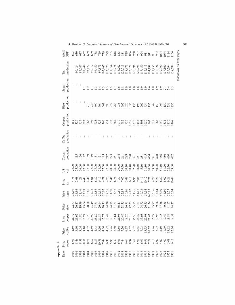
forced by data considerations if for no other reason. In Appendix A, we provide brief

details of the construction and sources for the production and income data that we use;

since this work is not easily reproduced, we also present the data. They include a

series for real world income, which runs from 1900 to 1987, and this is matched to

world production data for cocoa (from 1901), for coffee (from 1930), for copper, for

rice (from 1904), for sugar (from 1903), and for tin (from 1901). Average annual

prices for all of these goods are available from the same World Bank sources that were

used in our earlier work, and these were deflated, as before, by the US consumer price

index.

We begin by presenting some descriptive statistics in Table 1. Column 2 shows that the

deflated prices all had negative growth rates over most of the 20th century; this is the

well-researched decline in the terms of trade for primary commodities. However, it should

be noted from the next two columns that none of these trends are significantly different

from zero; even using the (smaller) standard error that allows for possible serial

correlation, in only one case, rice, is the estimated rate of decline larger than its standard

errors, and then only marginally so. The lack of significant trends is consistent with the

stationarity of the price predicted by the theory, though it is far from ruling out

nonstationary alternatives. Of course, the standard errors are large because the prices

are so variable, so that the findings in the top half of the table might be summarized by

saying that prices exhibit some downward trend, but the trend is small relative to

variability.

In contrast to prices, production levels tend to exhibit significant positive trends. All the

coefficients are positive, and except for coffee and tin, which each rose at less than 1% a


year, all are significantly different from zero. World income grew at 2.94% a year from

1900 to 1987, so that Table 1 is not inconsistent with the underlying Lewis view that, in

the long run, demand drives supply with no effect on price.

Table 2 reports the results of using unit root tests to investigate the stationarity

issues further. We show the results of regressions of the rates of growth of prices,

production, and world income on the lagged logarithm of the level, and five lagged

values of growth rates. For a series that is I(1), the coefficient q� 1 on the lagged

logarithm should be zero, and the comparison of the standard t-value against

appropriate critical values can be used to test the null of I(1). If the series is integrated

with nonzero drift, the t-statistic can be compared against the usual distribution; if there

is no drift, the critical values are nonstandard, and are given, for example, in Hamilton

(1994). It is also interesting to test the joint hypothesis that the drift is zero and the

coefficient on the lagged logarithm is zero, so that the series is I(1) without drift. The

F-statistic in the table is calculated in the usual way, and gives a test that is valid under

the null if compared against special critical values (see Hamilton, 1994 and the notes to

the table).

The major practical problem with all of these tests is lack of power; it is typically

difficult to reject the null, and failure to do so must not be taken as a confirmation. For

example, the top part of the table shows only two rejections, for cocoa and coffee, both

Table 1

Summary data on prices, production, and income

Commodity Dates covered Mean rate

of growth

Standard

error

Corrected

standard error

Prices

Cocoa 1901–1987 � 0.0084 0.029 0.023

Coffee 1901–1987 � 0.0004 0.026 0.020

Copper 1901–1987 � 0.0111 0.019 0.013

Rice 1901–1987 � 0.0168 0.021 0.015

Rubber 1948–1991 � 0.0254 0.054 0.024

Sugar 1901–1987 � 0.0197 0.040 0.026

Tin 1901–1987 � 0.0003 0.021 0.015

Production

Cocoa 1902–1988 0.0339 0.012 0.008

Coffee 1931–1990 0.0088 0.026 0.014

Copper 1901–1990 0.0333 0.014 0.008

Rice 1905–1987 0.0223 0.008 0.006

Rubber 1947–1990 0.0407 0.011 0.013

Sugar 1904–1994 0.0253 0.008 0.006

Tin 1902–1987 0.0048 0.016 0.009

World income

Income 1901–87 0.0294 0.004 0.004

The dates covered exclude the first observation lost to differencing. The mean rate of growth is the average of the

change in logarithms over the period shown. The standard errors are standard errors of the mean rate of growth, in

the first column ignoring serial correlation, and in the second, using the Newey–West procedure with 10 (annual)

lags.


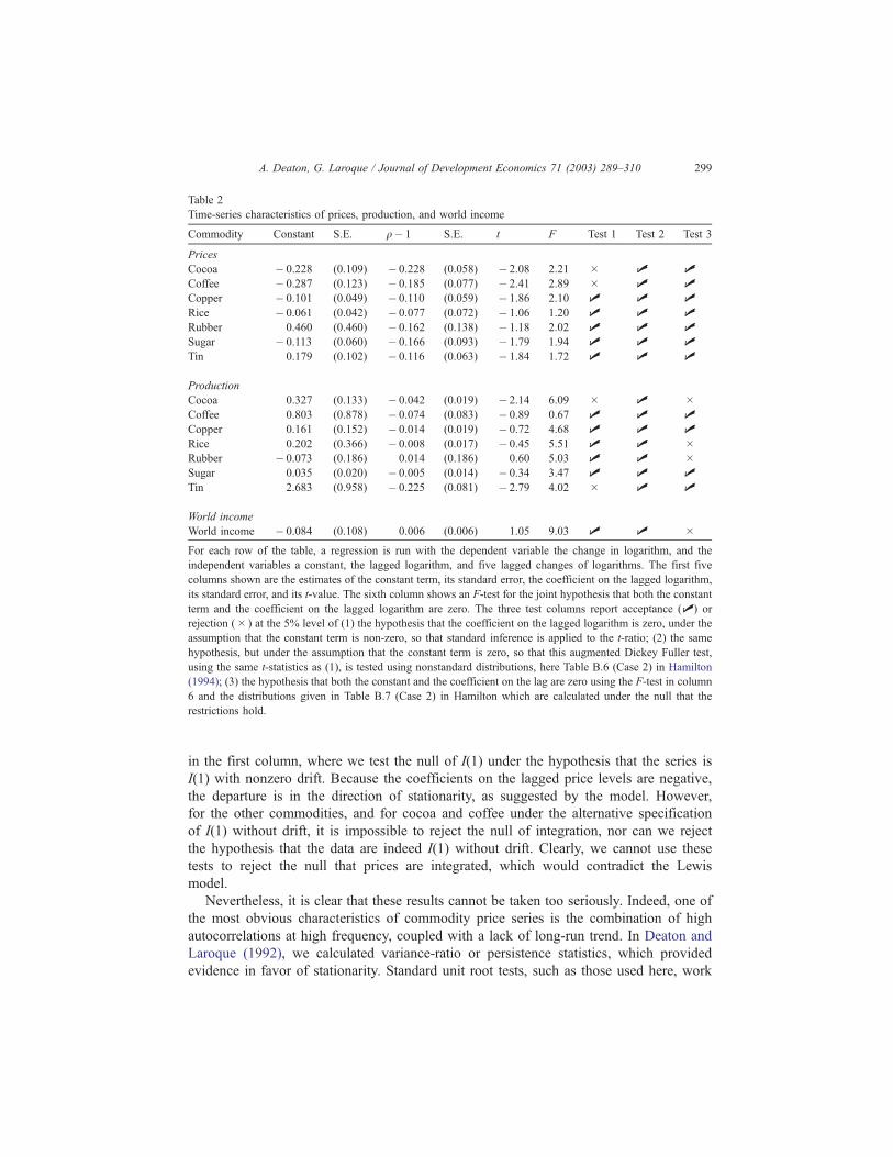
in the first column, where we test the null of I(1) under the hypothesis that the series is

I(1) with nonzero drift. Because the coefficients on the lagged price levels are negative,

the departure is in the direction of stationarity, as suggested by the model. However,

for the other commodities, and for cocoa and coffee under the alternative specification

of I(1) without drift, it is impossible to reject the null of integration, nor can we reject

the hypothesis that the data are indeed I(1) without drift. Clearly, we cannot use these

tests to reject the null that prices are integrated, which would contradict the Lewis

model.

Nevertheless, it is clear that these results cannot be taken too seriously. Indeed, one of

the most obvious characteristics of commodity price series is the combination of high

autocorrelations at high frequency, coupled with a lack of long-run trend. In Deaton and

Laroque (1992), we calculated variance-ratio or persistence statistics, which provided

evidence in favor of stationarity. Standard unit root tests, such as those used here, work

Table 2

Time-series characteristics of prices, production, and world income

Commodity Constant S.E. q� 1 S.E. t F Test 1 Test 2 Test 3

Prices

Cocoa � 0.228 (0.109) � 0.228 (0.058) � 2.08 2.21 � U UCoffee � 0.287 (0.123) � 0.185 (0.077) � 2.41 2.89 � U UCopper � 0.101 (0.049) � 0.110 (0.059) � 1.86 2.10 U U URice � 0.061 (0.042) � 0.077 (0.072) � 1.06 1.20 U U URubber 0.460 (0.460) � 0.162 (0.138) � 1.18 2.02 U U USugar � 0.113 (0.060) � 0.166 (0.093) � 1.79 1.94 U U UTin 0.179 (0.102) � 0.116 (0.063) � 1.84 1.72 U U U

Production

Cocoa 0.327 (0.133) � 0.042 (0.019) � 2.14 6.09 � U �Coffee 0.803 (0.878) � 0.074 (0.083) � 0.89 0.67 U U UCopper 0.161 (0.152) � 0.014 (0.019) � 0.72 4.68 U U URice 0.202 (0.366) � 0.008 (0.017) � 0.45 5.51 U U �Rubber � 0.073 (0.186) 0.014 (0.186) 0.60 5.03 U U �Sugar 0.035 (0.020) � 0.005 (0.014) � 0.34 3.47 U U UTin 2.683 (0.958) � 0.225 (0.081) � 2.79 4.02 � U U

World income

World income � 0.084 (0.108) 0.006 (0.006) 1.05 9.03 U U �For each row of the table, a regression is run with the dependent variable the change in logarithm, and the

independent variables a constant, the lagged logarithm, and five lagged changes of logarithms. The first five

columns shown are the estimates of the constant term, its standard error, the coefficient on the lagged logarithm,

its standard error, and its t-value. The sixth column shows an F-test for the joint hypothesis that both the constant

term and the coefficient on the lagged logarithm are zero. The three test columns report acceptance (U ) or

rejection (� ) at the 5% level of (1) the hypothesis that the coefficient on the lagged logarithm is zero, under the

assumption that the constant term is non-zero, so that standard inference is applied to the t-ratio; (2) the same

hypothesis, but under the assumption that the constant term is zero, so that this augmented Dickey Fuller test,

using the same t-statistics as (1), is tested using nonstandard distributions, here Table B.6 (Case 2) in Hamilton

(1994); (3) the hypothesis that both the constant and the coefficient on the lag are zero using the F-test in column

6 and the distributions given in Table B.7 (Case 2) in Hamilton which are calculated under the null that the

restrictions hold.


with a small number of lags, and are liable to miss the slow mean reversion that is

captured by the variance-ratio statistics. Note that the results in the top half of the table are

also consistent with stationary autoregressive models for prices. For example, the standard

errors on the lagged coefficient are such that for no commodity can we reject the

hypothesis that the coefficient on lagged price is 0.8, or � 0.2 for q� 1. The unit root

tests are essentially uninformative about the stationarity or otherwise of commodity

prices.

The unit root tests for production and for world income are presented in the bottom half

of the table. While they suffer from the same sort of problems as the price tests, there are

much larger and more obvious drifts in the production (and income) series, and the joint

tests for integration without drift reject in a number of cases. Of more concern are the

rejections of integration for cocoa and tin; while the rejection is marginal for the former,

the production of tin appears to be better represented by a stationary than a nonstationary

process.

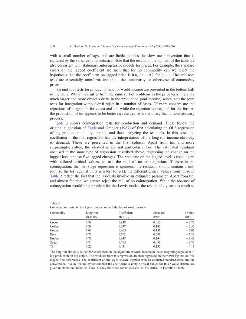
Table 3 shows cointegration tests for production and demand. These follow the

original suggestion of Engle and Granger (1987) of first calculating an OLS regression

of log production on log income, and then analyzing the residuals. In this case, the

coefficient in the first regression has the interpretation of the long-run income elasticity

of demand. These are presented in the first column. Apart from tin, and more

surprisingly, coffee, the elasticities are not particularly low. The estimated residuals

are used in the same type of regression described above, regressing the change on the

lagged level and on five lagged changes. The t-statistic on the lagged level is used, again

with tailored critical values, to test the null of no cointegration. If there is no

cointegration, the first-stage regression is spurious, the residuals should contain a unit

root, so the test against unity is a test for I(1); the different critical values from those in

Table 2 reflect the fact that the residuals involve an estimated parameter. Apart from tin,

and almost for rice, we cannot reject the null of no cointegration. While the absence of

cointegration would be a problem for the Lewis model, the results likely owe as much to

Table 3

Cointegration tests for the log of production and the log of world income

Commodity Long-run

elasticity

Coefficient

on ut� 1

Standard

error

t-value

for 1

Cocoa 0.89 0.848 0.055 � 2.75

Coffee 0.39 0.637 0.142 � 2.55

Copper 1.08 0.605 0.131 � 3.02

Rice 0.70 0.702 0.091 � 3.28

Rubber 0.78 0.648 0.144 � 2.45

Sugar 0.84 0.765 0.086 � 2.72

Tin 0.22 0.431 0.135 � 4.13

The long-run elasticity is the OLS coefficient on the logarithm of world income in the cointegrating regression of

log production on log output. The residuals from this regression are then regressed on their own lag and on five

lagged first differences. The coefficient on the lag is shown, together with its estimated standard error, and the

conventional t-value for the hypothesis that the coefficient is unity. Critical values for this t-value statistic are

given in Hamilton, Table B8, Case 2. Only the value for tin exceeds its 5% critical in Hamilton’s table.


lack of power as to any genuine failure of cointegration; in particular note that all the

estimated coefficients on ut� 1 are less than 0.85, and that five out of the seven are 0.7

or less.

The predictions of the Lewis model that prices are stationary and that quantities and

world demand are cointegrated are not obviously confirmed by these simple tests.

Prices are slow to revert to their long-run means, as are the ratios of commodity

production to world income. However, it is well known that such slow reversion is

poorly captured by tests that rely on a few low-order autocorrelations, and we take the

view that the descriptive tests are essentially neutral as far as the validity of the model

is concerned.

4. Results of estimating the model

Tables 4 and 5 show the reduced form and structural parameter estimates for each of the

goods, cocoa, coffee, and copper in Table 4, and rice, sugar, and tin in Table 5. For each

commodity, the top three panels present the reduced form parameters, for the price

equation, Eq. (16), for the production equation, Eq. (15), and for the world income

equation, Eq. (17). The row labeled ‘‘cointegrating’’ is the parameter estimate on the

cointegration term hyt � 1� qt � 1, the difference between (logarithmic) demand and

supply. Other rows correspond to the coefficients on lags of price, production change,

and income change. The fourth panel shows the estimate of the cointegrating constant u;this is the estimate of the long-run elasticity of demand, already estimated by the two-step

Engle–Granger procedure in Table 3. The final panel shows the structural parameters for

the supply equation—the demand equation is not identified except for the long-run

elasticity from the cointegrating relationship.

Except for rice, for which we could only obtain sensible results with a single lag, we

show results with two lags of prices, production and world income growth. We tested the

overidentification restrictions (Eq. (18)) using likelihood ratio tests from FIML estimation

with and without the restrictions. The restrictions easily passed the test for all of the

commodities, and we present only the restricted estimates, which allow us to recover

unique estimates for the structural parameters.

The cointegrating parameters provide elasticities of demand that are not very different

from those shown in Table 3, and which range from 1.03 for copper and 0.90 to cocoa, to

0.48 for coffee and 0.15 for tin. All of these are quite precisely estimated, with standard

errors between 0.04 and 0.08.

The estimated coefficients of the cointegrating term in the production and price

equations are all positive, and for each good, at least one of the coefficients is significantly

different from zero. Conditional on lagged prices, production, and world income, an

imbalance between lagged demand and lagged supply leads to an increase in price, or

output, or both. Although the demand equation is not identified, the model predicts what

we see, that these reduced form coefficients be positive, when the cointegration term does

not enter the world income equation and the coefficients B(0) and D(0) are both positive.

To see this, note first that from the world income estimates in the third panel, we see that in

no case are there significant effects of the cointegrating term, lagged quantity changes, or


lagged prices, an absence that can be formally confirmed by likelihood ratio tests. Suppose

then that all of these coefficients are zero. Then use Eq. (17) to substitute for

yt=Dyt+ yt� 1 in Eqs. (11) and (12) which yields, after some manipulation, Eqs. (15)

Table 4

Reduced form and structural estimates of cocoa, coffee, and copper

Cocoa Coffee Copper

Coefficient S.E. Coefficient S.E. Coefficient S.E.

Price

Constant � 4.35 (1.93) 0.13 (0.44) � 4.44 (1.55)

Cointegrating 0.36 (0.16) 0.25 (0.13) 0.37 (0.13)

pt� 1 0.94 (0.12) 0.80 (0.14) 1.10 (0.12)

pt� 2 � 0.22 (0.12) 0.03 (0.14) � 0.23 (0.12)

Dqt � 1 0.21 (0.30) 0.15 (0.20) � 0.07 (0.16)

Dqt � 2 0.08 (0.27) 0.08 (0.18) 0.09 (0.15)

Dyt� 1 � 0.35 (0.53) 0.08 (0.45) 0.36 (0.38)

Dyt� 2 � 0.76 (0.57) � 1.33 (0.66) � 0.19 (0.35)

R2/no. of observations 0.79 84 0.78 45 0.81 85

Production

Constant � 1.05 (0.70) 0.55 (0.39) � 5.43 (1.29)

Cointegrating 0.11 (0.06) 0.24 (0.09) 0.46 (0.10)

pt� 1 � 0.05 (0.04) � 0.36 (0.08) 0.16 (0.10)

pt� 2 0.05 (0.04) 0.46 (0.08) � 0.21 (0.09)

Dqt � 1 � 0.46 (0.11) � 0.59 (0.12) 0.09 (0.13)

Dqt � 2 � 0.22 (0.10) � 0.13 (0.11) 0.17 (0.12)

Dyt� 1 0.10 (0.16) 0.07 (0.43) 0.45 (0.46)

Dyt� 2 � 0.22 (0.18) � 1.26 (0.45) � 0.23 (0.44)

R2 0.26 0.65 0.29

World income

Constant 0.57 (0.29) � 0.04 (0.10) � 0.39 (0.35)

Cointegrating � 0.05 (0.03) � 0.06 (0.02) 0.03 (0.03)

pt� 1 0.02 (0.02) 0.02 (0.01) � 0.04 (0.03)

pt� 2 � 0.00 (0.02) � 0.00 (0.01) 0.03 (0.03)

Dqt � 1 0.02 (0.04) � 0.07 (0.03) 0.03 (0.04)

Dqt � 2 0.04 (0.04) � 0.04 (0.02) 0.02 (0.04)

Dyt� 1 0.43 (0.11) 0.51 (0.11) 0.48 (0.13)

Dyt� 2 � 0.12 (0.11) � 0.27 (0.11) � 0.16 (0.13)

R2 0.24 0.39 0.21

Cointegration

Dyt� 1 0.90 (0.05) 0.48 (0.08) 1.03 (0.04)

D0 0.29 (0.23) 0.95 (0.49) 1.25 (0.37)

D1 � 0.32 (0.24) � 1.01 (0.47) � 1.22 (0.44)

D2 0.11 (0.07) 0.43 (0.15) 0.08 (0.16)

Total 0.08 (0.04) 0.27 (0.10) 0.12 (0.07)

E0 � 0.53 (0.16) � 0.73 (0.20) 0.18 (0.18)

E1 � 0.24 (0.15) � 0.21 (0.20) 0.06 (0.14)

Total � 0.77 (0.33) � 0.94 (0.59) 0.24 (0.50)


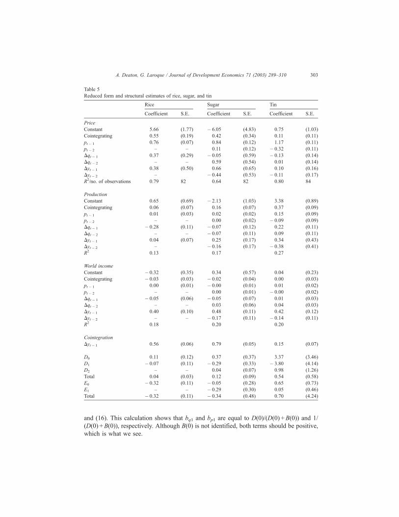
and (16). This calculation shows that bq1 and bp1 are equal to D(0)/(D(0) +B(0)) and 1/

(D(0) +B(0)), respectively. Although B(0) is not identified, both terms should be positive,

which is what we see.

Table 5

Reduced form and structural estimates of rice, sugar, and tin

Rice Sugar Tin

Coefficient S.E. Coefficient S.E. Coefficient S.E.

Price

Constant 5.66 (1.77) � 6.05 (4.83) 0.75 (1.03)

Cointegrating 0.55 (0.19) 0.42 (0.34) 0.11 (0.11)

pt� 1 0.76 (0.07) 0.84 (0.12) 1.17 (0.11)

pt� 2 – – 0.11 (0.12) � 0.32 (0.11)

Dqt� 1 0.37 (0.29) � 0.05 (0.59) � 0.13 (0.14)

Dqt� 2 – – 0.59 (0.54) 0.01 (0.14)

Dyt� 1 0.38 (0.50) 0.66 (0.65) 0.10 (0.16)

Dyt� 2 – � 0.44 (0.53) � 0.11 (0.17)

R2/no. of observations 0.79 82 0.64 82 0.80 84

Production

Constant 0.65 (0.69) � 2.13 (1.03) 3.38 (0.89)

Cointegrating 0.06 (0.07) 0.16 (0.07) 0.37 (0.09)

pt� 1 0.01 (0.03) 0.02 (0.02) 0.15 (0.09)

pt� 2 – – 0.00 (0.02) � 0.09 (0.09)

Dqt� 1 � 0.28 (0.11) � 0.07 (0.12) 0.22 (0.11)

Dqt� 2 – – � 0.07 (0.11) 0.09 (0.11)

Dyt� 1 0.04 (0.07) 0.25 (0.17) 0.34 (0.43)

Dyt� 2 – � 0.16 (0.17) � 0.38 (0.41)

R2 0.13 0.17 0.27

World income

Constant � 0.32 (0.35) 0.34 (0.57) 0.04 (0.23)

Cointegrating � 0.03 (0.03) � 0.02 (0.04) 0.00 (0.03)

pt� 1 0.00 (0.01) � 0.00 (0.01) 0.01 (0.02)

pt� 2 – – 0.00 (0.01) � 0.00 (0.02)

Dqt� 1 � 0.05 (0.06) � 0.05 (0.07) 0.01 (0.03)

Dqt� 2 – – 0.03 (0.06) 0.04 (0.03)

Dyt� 1 0.40 (0.10) 0.48 (0.11) 0.42 (0.12)

Dyt� 2 – – � 0.17 (0.11) � 0.14 (0.11)

R2 0.18 0.20 0.20

Cointegration

Dyt� 1 0.56 (0.06) 0.79 (0.05) 0.15 (0.07)

D0 0.11 (0.12) 0.37 (0.37) 3.37 (3.46)

D1 � 0.07 (0.11) � 0.29 (0.33) � 3.80 (4.14)

D2 – – 0.04 (0.07) 0.98 (1.26)

Total 0.04 (0.03) 0.12 (0.09) 0.54 (0.58)

E0 � 0.32 (0.11) � 0.05 (0.28) 0.65 (0.73)

E1 – – � 0.29 (0.30) 0.05 (0.46)

Total � 0.32 (0.11) � 0.34 (0.48) 0.70 (4.24)


The lagged values of the growth of world income are generally insignificantly different

from zero in the reduced form estimates, the only exception being Dyt� 2 in the copper

equation. These weak results are worth noting because the acceptance of the over-

identification test depends on them. Although we can accept the overidentification that

comes from exclusion of world demand from the supply Eq. (2), world demand plays such

a limited role beyond its effects in the cointegrating term that the test is quite

unimpressive.

World income is well modeled as an AR(1) in first-differences with an autocorrelation

coefficient of 0.4. Lagged prices, lagged production growth, and shortfall of supply over

demand have essentially no detectable effects on the rate of growth of world income,

something that can be confirmed by a series of Granger noncausality tests, all of which are

easily passed. This result is perhaps not surprising given the limited importance of these

commodity markets in the world economy.

The response of supply to price is detailed in the bottom panel which shows the

structural estimates of the supply equation. A pattern that is repeated across all of the

commodities is one in which there is a positive instantaneous effect of price on production,

followed by a negative effect at one lag. At the third lag, the response is in all case positive

(except for rice where it is constrained to be zero) and the sum of the responses is (again in

all cases) positive. However, once again, although the signs are right, the results are not

always significantly different from zero, and we find a significantly positive long-run price

response of the growth of supply for only cocoa and coffee. The offsetting effects in the

first and second period can perhaps be attributed to the existence of a short supply

response in which the level of supply responds to the level of prices, so that the growth of

supply is linked to the growth of prices. This short-run response might be linked to

inventory behavior. Since it is extremely difficult to obtain accurate data on inventories,

the production series that we use are almost certainly in part consumption series. If so, and

if price increases elicits a short-run response out of inventories, there will appear to be a

short-run response of ‘‘production’’ to price.

The Lewis model postulates that long-run supply is infinitely elastic, so that the

elasticity we are interested in here is by how much the rate of growth of production

responds to a difference between the current price and the long-run equilibrium price.

These elasticities are computed by dividing the sum of the supply coefficients (shown as

‘‘total’’) in the last panel by one plus the sum of the coefficients on the lagged Dy terms.

Apart from tin, where all the supply parameters are very imprecisely estimated, and

which has an (absurd) estimated supply elasticity of 1.8, these elasticities lie in a sensible

range, ranging from 0.03 for rice to 0.16 for copper. According to the last, for example,

the rate of growth of supply will be 0.16 percentage points higher (from say, 2% a year to

2.16% a year) for every percentage point that the copper price exceeds its long-run

equilibrium. Only for cocoa and coffee do these estimates approach statistical signifi-

cance.

The final panel shows an important difference between the supply functions for the

foods (cocoa, coffee, rice, and sugar) and those for minerals (copper and tin). For the

foods, the estimated coefficients on the lagged production growth terms are negative,

and in most cases significantly so, while for the minerals, the coefficients are

insignificantly positive. Such findings are consistent with the view that, for agricultural


crops, the most important shocks are weather shocks, which are transitory, while for

minerals, permanent shocks are likely to be dominant. If we look back to Eq. (3), such

a pattern would induce what we see here, which is negative serial correlation in growth

rates for agricultural crops, because the changes in the weather from one year to

another is itself serially correlated, with little or no serial correlation for minerals, where

the shocks are permanent, with no supposition of negative autocorrelation in the

differences.

5. Summary and conclusions

We have proposed a statistical model of commodity prices based on Sir Arthur Lewis’

account in which the price of tropical produce is held down by the existence of unlimited

supplies of labor in tropical countries. In our version of the model, prices are stationary

around a long-run trend, production is cointegrated with world income, and the rate of

growth of supply responds to deviations of price from its long-run equilibrium. We have

fitted this model to long-run data for six commodities, cocoa, coffee, copper, rice, sugar,

and tin, over (some subset) of the years 1900–1987.

Our final assessment of the model is mixed. The results of Tables 4 and 5 can

certainly be interpreted in a Lewis framework. The deviation of long-run demand from

long-run supply exerts upward pressure on both price and production and, except for

one commodity (tin), the rate of growth of supply responds positively to deviations of

price from its long-run value. However, only for coffee and cocoa are these long-run

supply effects significantly different from zero. In spite of the enormous growth of

world income in the 20th century, the associated increase in supply has been forth-

coming without an increase in the real price of these commodities. As Lewis predicted,

increases in the real commodity prices must wait for the elimination of poverty in the

tropics.

However, it should also be noted that we have not succeeded in providing any

crucial evidence or piece of evidence that would convert a skeptic to the Lewis story.

The lack of long-run trend in commodity prices is a remarkable fact that is consistent

with the Lewis’ account, but as far as our model is concerned, we used the insight in

constructing the model, so that its success cannot be counted as any additional support

for our formulation. One source of difficulty is that the reversion of prices to their

long-run base is very slow, so that even a century of data is not enough to give clear

results on either the stationarity of prices or the cointegration of production and output,

and the empirical evidence is never very clear in rejecting alternatives. We saw in

Section 3 that the mechanical application of standard unit root tests would lead to the

conclusion that prices are integrated processes, something that can easily be interpreted

in terms of the low power of such tests, especially against slow mean reversion.

Nevertheless, we are left without any direct statistical support for the model from the

time-series tests.

The more detailed results in Tables 3 and 4, while consistent with the Lewis model,

suffer from lack of statistical significance, and the fits of the models come mostly from

the univariate time-series representations that are of little interest in the current context.


The exceptions are cocoa and coffee, the two commodities whose production is

confined to the tropics, and for which the Lewis model is most obviously consistent

with the data. For all the commodities, the price equations fit well, but only because

we are working in levels and regressing price on its own lag. As in our work on

speculative storage, our ‘‘explanation’’ of the autocorrelation of prices is essentially an

assumed autoregressive process. The production and world income equations are

essentially autoregressions in first-differences, and the terms of interest play a relatively

minor role. We have spent a great deal of time trying to dissect these results further, to

find a crucial piece of evidence that would either support the model, by being hard to

interpret without it, or else would refute it. However, as is often the case with

economic time-series, it is hard to find clear cut evidence that would convince a true

skeptic.

Acknowledgements

We are grateful to Mark Watson for helpful discussions during the preparation of this

paper and to Seth Carpenter for assistance in gathering data. We have benefited from

helpful referee reports and from comments by an editor.

Appendix A. Data and sources

We use three types of data, on world income, on prices, and on production. World

income data come from Maddison (1989). Maddison’s book has annual series on GDP

for 16 (current OECD) countries from 1900 to 1987. To make them comparable, he

uses purchasing power parity conversion figures from the OECD and Eurostat for the

OECD countries to yield ‘‘international dollars’’ used for conversion of domestic levels.

The series have been converted to indices which are then linked to the 1980

benchmark international dollar figure to create an internationally comparable series

for each country which can then be summed over countries. The series shown in the

table is in billions of 1980 constant dollars. Price data come from the World Bank, and

were first used in the study by Grilli and Yang (1988). They are shown as index

numbers, as is the US consumer price index. The production data come from a wide

range of sources, which are briefly summarized here. Recent annual data on crops (here

cocoa, coffee, rice, and sugar) can be readily obtained from the FAO website, http://

www.fao.org. Cocoa production comes from various issues of Gill and Duffus’ serial

Cocoa Statistics: the units in the table are thousands of metric tons. Coffee data come

from the Brazil’s Departamento Nacional do Cafe’s Annual Statistics: the units are

thousands of 60 kg bags. Data on copper production are taken from the serial

Metallstatistik: units are thousands of metric tons. Rice production comes from the

FAO, with historical data from FAO (1965); units are millions of quintals. Historical

data on sugar are available in FAO (1961); units are hundreds of millions of quintals.

Tin production comes from various yearbooks of the International Tin Council; units

are metric tons.


Date

Price

cocoa

Price

coffee

Price

copper

Price

rice

Price

sugar

Price

tin

US

cpi

Cocoa

production

Coffee

production

Copper

production

Rice

production

Sugar

production

Tin

production

World

GDP

1900

8.99

4.59

21.72

22.77

33.19

4.78

25.00

––

452

––

–603

1901

8.46

3.60

21.62

20.47

26.86

2.68

25.00

115

–529

––

90,424

630

1902

8.51

3.04

14.80

19.79

21.46

4.28

26.00

126

–557

––

85,547

637

1903

8.56

3.10

17.77

25.04

22.99

4.49

27.00

127

–593

–1.1

91,948

657

1904

8.78

4.32

17.20

20.88

30.61

4.48

27.00

159

–662

718

1.2

93,472

659

1905

8.62

4.59

20.92

23.49

32.72

5.01

27.00

149

–693

733

1.1

96,012

689

1906

8.83

4.43

25.87

27.61

24.86

6.37

27.00

151

–725

690

1.3

98,450

738

1907

10.71

3.50

26.84

29.64

26.15

6.10

28.00

151

–725

704

1.4

99,873

759

1908

7.44

4.60

17.73

30.75

30.02

4.71

27.00

195

–766

661

1.3

105,867

729

1909

6.37

4.87

17.42

24.20

29.55

4.75

27.00

212

–851

690

1.5

112,370

779

1910

5.99

5.76

17.10

24.15

31.90

5.46

28.00

223

–872

977

1.5

111,354

785

1911

6.32

7.80

16.61

31.61

35.42

6.76

28.00

251

–887

963

1.7

112,776

818

1912

6.69

8.86

21.93

36.47

30.61

7.37

29.00

244

–1019

1035

1.6

118,262

853

1913

7.44

7.20

20.49

28.55

22.87

7.07

29.70

261

–982

992

1.8

127,711

881

1914

6.64

6.37

18.25

26.91

30.96

5.48

30.10

289

–926

1020

1.9

118,872

829

1915

8.94

5.32

23.19

27.25

38.82

6.17

30.40

290

–1058

1035

1.8

122,022

856

1916

7.60

5.87

36.50

25.15

51.25

6.95

32.70

321

–1376

1135

1.8

120,396

930

1917

5.99

5.65

36.47

21.71

54.18

9.88

38.40

351

–1443

1193

1.8

120,294

907

1918

6.90

7.03

33.05

24.72

49.73

14.19

45.10

281

–1395

1207

1.9

117,450

924

1919

9.96

13.73

25.08

26.55

59.34

10.12

51.80

445

–1050

934

1.9

115,113

911

1920

7.28

10.57

23.43

31.24

140.15

7.72

60.00

404

–967

1135

1.6

114,198

911

1921

4.17

5.76

16.77

35.77

36.36

4.78

53.60

371

–528

1049

1.8

111,455

901

1922

4.92

7.92

17.95

39.56

32.84

5.20

50.20

428

–863

1150

1.9

115,824

962

1923

4.07

8.19

19.35

37.56

58.99

6.82

51.10

456

–1250

1293

1.9

119,990

1024

1924

4.07

11.79

17.47

40.85

44.80

8.02

51.20

486

–1331

1150

2.1

137,160

1074

1925

5.08

13.62

18.84

41.17

26.27

9.26

52.50

490

–1410

1236

2.4

139,294

1114

1926

6.16

12.34

18.52

44.27

26.04

10.44

53.00

472

–1468

1236

2.5

138,684

1156

(continued

onnextpage)

Appendix

A


Date

Price

cocoa

Price

coffee

Price

copper

Price

rice

Price

sugar

Price

tin

US

cpi

Cocoa

production

Coffee

production

Copper

production

Rice

production

Sugar

production

Tin

production

World

GDP

1927

8.46

10.35

17.34

41.01

30.96

10.29

52.00

530

–1513

1221

2.4

155,245

1184

1928

6.85

12.84

19.55

37.10

25.57

8.06

51.30

507

–1716

1221

2.6

173,736

1221

1929

5.57

12.23

24.30

37.03

20.17

7.22

51.30

551

–1948

1265

2.8

192,227

1274

1930

4.39

7.14

17.42

29.17

14.43

5.07

50.00

540

41,021

1596

1236

2.8

174,854

1200

1931

2.78

4.87

10.90

16.37

13.02

3.91

45.60

532

29,396

1387

1308

2.9

140,310

1123

1932

2.36

5.87

7.46

14.40

8.33

3.52

40.90

557

41,491

897

1279

2.4

94,082

1048

1933

2.36

5.04

9.42

12.23

11.37

6.25

38.80

628

33,767

1008

1279

2.2

81,178

1063

1934

2.78

6.14

11.31

15.91

13.96

8.34

40.10

590

43,028

1267

1394

2.3

114,198

1117

1935

2.68

4.93

11.61

20.79

18.53

8.06

41.10

701

31,577

1467

1244

2.3

130,658

1181

1936

3.64

5.26

12.71

20.41

20.29

7.42

41.50

737

36,653

1696

1332

2.5

173,025

1283

1937

4.50

6.09

17.67

21.63

20.64

8.69

43.00

758

42,583

2285

1417

2.7

197,815

1353

1938

2.78

4.26

13.42

19.85

17.01

6.76

42.20

736

39,171

2010

1317

2.7

154,229

1351

1939

2.57

4.10

14.71

19.21

17.71

8.05

41.60

807

38,024

2124

1323

2.7

157,683

1447

1940

2.73

3.93

15.16

23.09

15.95

7.97

42.00

690

32,220

2397

1323

2.9

227,381

1495

1941

4.07

6.26

15.83

25.81

19.82

8.32

44.10

672

26,120

2525

1221

2.8

243,535

1625

1942

4.76

7.42

15.81

28.35

29.67

8.31

48.80

677

26,348

2672

1260

2.7

117,145

1776

1943

4.76

7.42

15.81

29.63

28.62

8.31

51.80

612

25,923

2693

1228

2.5

137,363

1945

1944

4.76

7.42

15.81

29.63

28.97

8.31

52.70

572

24,484

2509

1298

2.6

99,568

1995

1945

4.76

7.53

15.81

29.63

34.48

8.31

53.90

620

22,144

2172

1254

2.3

87,376

1838

1946

6.16

10.24

18.54

34.18

41.63

8.72

58.50

660

25,675

1848

1129

2.2

87,681

1631

1947

18.68

14.78

28.12

54.72

56.29

12.46

66.90

623

29,296

2229

1394

2.5

109,423

1656

1948

21.25

15.00

29.57

57.99

49.61

15.87

72.10

599

27,917

2323

1416

3.0

149,555

1746

1949

11.56

18.10

25.76

50.08

48.79

15.88

71.40

783

30,918

2268

1553

2.8

159,918

1807

1950

17.18

25.86

28.50

42.24

58.40

15.27

72.10

768

28,911

2525

1572

2.9

164,897

1950

1951

19.00

30.52

32.47

44.61

66.50

20.32

77.80

813

30,285

2662

1705

3.3

165,100

2116

1952

18.95

29.48

32.47

48.29

48.91

19.26

79.50

652

29,725

2766

1832

3.6

167,945

2200

1953

19.86

29.48

38.64

53.98

39.99

15.32

80.10

811

32,297

2802

1979

3.5

172,822

2304

1954

30.94

39.83

39.84

48.79

38.23

14.68

80.50

788

32,016

2852

1942

3.9

171,704

2340

1955

20.07

31.03

50.30

43.72

38.00

15.15

80.20

815

33,922

3112

2098

3.8

170,688

2484

Appendix

A(continued

)


1956

14.61

35.69

56.11

42.30

40.81

16.21

81.40

855

43,670

3470

2197

4.0

169,062

2570

1957

16.38

35.17

39.69

42.39

60.52

15.39

84.30

911

34,582

3556

2165

4.2

165,710

2648

1958

23.71

25.86

34.57

43.97

41.05

15.21

86.60

786

46,230

3449

2241

4.5

117,653

2674

1959

19.59

22.24

41.84

40.84

34.83

16.32

87.30

923

52,001

3693

2199

5.2

121,107

2826

1960

15.20

21.21

43.00

38.53

36.83

16.22

88.69

1053

66,421

4242

2189

5.0

138,684

2961

1961

12.10

19.66

40.15

42.17

34.13

18.12

89.57

1189

52,814

4394

2158

5.5

138,684

3095

1962

11.24

18.62

41.06

47.21

34.95

18.33

90.68

1140

58,275

4555

2266

5.2

143,967

3255

1963

13.54

18.10

41.06

44.27

99.69

18.65

91.75

1176

53,416

4624

2470

5.3

143,500

3420

1964

12.53

24.31

42.88

42.54

68.85

25.20

92.99

1234

56,891

4799

2629

6.0

149,200

3609

1965

9.26

23.79

46.99

42.11

24.86

28.49

94.47

1508

35,878

4963

2543

6.5

155,100

3821

1966

13.06

21.72

48.53

50.42

21.81

26.23

97.29

1226

66,359

5220

2612

6.4

167,100

4015

1967

15.58

20.17

51.30

63.59

23.34

24.53

100.00

1351

44,443

5060

2778

6.7

172,900

4155

1968

18.41

20.17

56.15

62.29

23.22

23.69

104.22

1354

51,721

5459

2891

6.7

183,100

4384

1969

24.46

20.69

63.78

57.74

39.52

26.30

109.85

1242

43,410

5943

2956

7.0

178,000

4605

1970

18.31

26.90

77.42

44.49

43.98

27.85

116.35

1435

48,078

6403

3167

7.3

186,700

4748

1971

14.34

23.28

69.01

39.86

53.01

26.76

121.27

1499

40,154

6477

3181

7.4

188,100

4916

1972

17.29

25.86

67.92

45.45

87.14

28.37

125.26

1583

53,083

7063

3082

7.6

196,300

5165

1973

34.47

32.07

78.99

108.14

112.94

36.38

133.05

1398

57,166

7511

3362

7.8

189,100

5459

1974

52.51

34.14

102.85

167.46

351.36

63.36

147.76

1448

43,792

7576

3333

7.9

183,600

5485

1975

40.04

33.62

85.26

112.18

240.42

54.33

161.25

1548

62,433

7182

3591

8.2

181,200

5461

1976

58.50

73.97

92.34

78.63

135.81

60.73

170.49

1510

54,307

7658

3504

8.2

180,200

5725

1977

108.39

124.66

88.30

84.10

95.23

85.47

181.59

1339

42,777

7854

3723

9.0

188,600

5930

1978

97.41

85.86

87.90

113.54

91.48

100.66

195.41

1503

52,571

7671

3881

9.1

196,700

6180

1979

94.20

89.48

123.79

102.36

113.29

113.87

217.46

1495

60,028

7765

3773

8.9

200,100

6374

1980

74.40

80.69

137.37

134.06

336.24

135.26

246.85

1626

62,258

7786

3993

8.5

200,000

6456

1981

59.41

66.21

112.38

149.23

198.90

115.51

272.36

1660

66,064

8355

4125

9.3

204,600

6610

1982

49.60

72.42

97.79

90.53

99.05

104.53

289.12

1734

77,311

8041

4239

10.1

190,600

6578

1983

60.57

68.05

104.44

85.60

99.53

103.07

298.46

1523

62,366

8048

4518

9.7

173,000

6769

1984

70.11

74.55

89.58

77.93

61.31

99.73

311.15

1513

67,676

8236

4702

9.9

167,100

7107

1985

65.66

75.53

87.98

66.74

48.09

94.66

322.23

1944

67,449

8380

4734

9.8

158,200

7339

1986

60.98

100.52

86.67

65.54

73.03

58.56

328.40

1961

74,764

8466

4739

10.0

141,300

7541

1987

58.76

58.66

112.46

71.71

81.56

63.58

340.39

1994

57,569

8742

4575

10.4

136,300

7759


References

Ahn, S.K., Reinsel, G.C., 1990. Estimation of partially non-stationary autoregressive models. Journal of the

American Statistical Association 85, 813–823.

Brazil, Departamento Nacional do Cafe. Anuario Estatistico, various years.

Deaton, A., Laroque, G., 1992. On the behavior of commodity prices. Review of Economic Studies 59, 1–24.

Deaton, A., Laroque, G., 1996. Competitive storage and commodity price dynamics. Journal of Political Econ-

omy 104, 896–923.

Engle, R.F., Granger, C.W.J., 1987. Co-Integration and error correction: representation, testing, and estimation.

Econometrica 55, 251–276.

Food and Agricultural Organization, 1961. The World Sugar Economy in Figures. Commodities Division, Rome.

Food and Agricultural Organization, 1965. The World Rice Economy in Figures. Commodities Division, Rome.

Gill and Duffus. Cocoa statistics. London, various years.

Gray, L.C., 1914. Rent under the assumptions of exhaustibility. Quarterly Journal of Economics 28, 466–489.

Grilli, E., Yang, M.C., 1988. Primary commodity prices, manufactured goods prices, and the terms of trade in

developing countries. World Bank Economic Review 2, 1–47.

Halvorsen, R., Smith, T.R., 1991. A test of the theory of exhaustible resources. Quarterly Journal of Economics

106, 123–140.

Hamilton, J.D., 1994. Time-Series Analysis. Princeton Univ. Press, Princeton.

Hotelling, H., 1931. The economics of exhaustible resources. Journal of Political Economy 39, 137–175.

International Tin Council. Tin Statistics. London, annual.

Lewis, A., 1954. Economic development with unlimited supplies of labor. Manchester School 22, 139–191.

Maddison, A., 1989. The World Economy in the 20th Century. OECD, Paris.

Metallstatistik: Metallgesellschaft Aktiengesellschaft: Frankfurt am Main. Die Gesellschaft.

Prebisch, R., 1959. International trade and payments in an era of coexistence: commercial policy in the under-

developed countries. American Economic Review (Papers and Proceedings) 49, 251–273.

Singer, H.W., 1950. US Foreign investment in underdeveloped areas: the distribution of gains between investing

and borrowing countries. American Economic Review (Papers and Proceedings) 40, 473–485.

Watson, M.W., 1994. Vector autoregressions and cointegration. Chapter 47. In: Engle, R.F., McFadden, D.L.

(Eds.), Handbook of Econometrics, vol. 4. North-Holland, Amsterdam, pp. 2843–2915.


a model of commodity prices after sir arthur lewisdeaton/downloads/a_model_of... · a model of...

Documents