HAL Id: hal-01948174https://hal.inria.fr/hal-01948174v1

Preprint submitted on 7 Dec 2018 (v1), last revised 17 May 2019 (v3)

HAL is a multi-disciplinary open accessarchive for the deposit and dissemination of sci-entific research documents, whether they are pub-lished or not. The documents may come fromteaching and research institutions in France orabroad, or from public or private research centers.

L’archive ouverte pluridisciplinaire HAL, estdestinée au dépôt et à la diffusion de documentsscientifiques de niveau recherche, publiés ou non,émanant des établissements d’enseignement et derecherche français ou étrangers, des laboratoirespublics ou privés.

A model of brain morphological changes caused by agingand Alzheimer’s disease for cross-sectional assessmentsRaphaël Sivera, Hervé Delingette, Marco Lorenzi, Xavier Pennec, Nicholas

Ayache

To cite this version:Raphaël Sivera, Hervé Delingette, Marco Lorenzi, Xavier Pennec, Nicholas Ayache. A model of brainmorphological changes caused by aging and Alzheimer’s disease for cross-sectional assessments. 2018.�hal-01948174v1�

A model of brain morphological changes caused by agingand Alzheimer’s disease for cross-sectional assessments

Raphaël Sivera∗1, Hervé Delingette1, Marco Lorenzi1, Xavier Pennec1, and NicholasAyache1

for the Alzheimer’s Disease Neuroimaging Initiative†

1Epione Research Project, Université Côte d’Azur, Inria Sophia Antipolis, France.

December 7, 2018

AbstractIn this study we propose a deformation-based framework to jointly model the influence of agingand Alzheimer’s disease (AD) on the brain morphological evolution. Our approach combines aspatio-temporal description of both processes into a generative model. A reference morphology isdeformed along specific trajectories to match subject specific morphologies. It is used to define twoimaging progression markers: 1) a morphological age and 2) a disease score. These markers can becomputed locally in any brain region.

The approach is evaluated on brain structural magnetic resonnance images (MRI) from theADNI database. The generative model is first estimated on a control population, then, for eachsubject, the markers are computed for each acquisition. The longitudinal evolution of these markersis then studied in relation with the clinical diagnosis of the subjects and used to generate possiblemorphological evolution.

In the model, the morphological changes associated with normal aging are mainly found aroundthe ventricles, while the Alzheimer’s disease specific changes are more located in the temporal lobeand the hippocampal area. The statistical analysis of these markers highlights differences betweenclinical conditions even though the inter-subject variability is quiet high. In this context, the modelcan be used to generate plausible morphological trajectories associated with the disease.

Our method gives two interpretable scalar imaging biomarkers assessing the effects of agingand disease on brain morphology at the individual and population level. Our proposed progressions∗Corresponding author at: Epione Research Project, INRIA Sophia-Antipolis, 2004, route des Lucioles, 06902

Sophia-Antipolis, France, raphael.sivera@inria.fr†Data used in preparation of this article were obtained from the Alzheimer’s Disease Neuroimaging Initiative

(ADNI) database (adni.loni.usc.edu). As such, the investigators within the ADNI contributed to the design andimplementation of ADNI and/or provided data but did not participate in analysis or writing of this report. Acomplete listing of ADNI investigators can be found at: http://adni.loni.usc.edu/wp-content/uploads/how_to_apply/ADNI_Acknowledgement_List.p

1

markers confirm an acceleration of apparent aging for Alzheimer’s subjects and can help discriminateclinical conditions even in prodromal stages. More generally, the joint modeling of normal andpathological evolutions shows promising results to describe age-related brain diseases over longtime scales.

Keywords: normal aging, Alzheimer’s disease, registration based framework, spatio-temporalmodel, cross-sectional progression markers, morphological age, disease score, imaging biomarkers.

1 IntroductionAge-related diseases are a growing public health concern with the aging of the population. Aprecise description of aging would be useful to predict and describe the evolution of these diseases.In complement to the chronological age, i.e. the time elapsed since birth, one would like to estimatea biological age that reflects the current physiological, functional or structural status of an organrelatively to the aging changes. However there is no unified way to describe aging in a clinical contextsince aging is a complex process which affects every part of the body with specific mechanisms andspecific rate. As a consequence multiple theories of aging have been proposed [1], leading to thedefinition of surrogate age variables based on the quantification of the biological changes.

1.1 Modeling brain morphological agingIn this paper we focus on the aging of the brain based on the study of its shape evolution. The brainis not exempt from aging and a decline of cognitive processing speed, working memory, inhibitoryfunction, and long-term memory is generally observed. This decline has been associated with neuralactivity changes [2] and it was also shown to be directly correlated with structural changes such asbrain atrophy and decrease of white matter integrity [3, 4].

The normal brain morphology has been studied from the development stage to the most advancedages in image-based studies. Measurements of brain structures (volumes, cortical thickness, etc.)have been performed for wide age ranges and the statistical analysis of the evolution of thesemeasurements led to an initial understanding of the normal brain shape evolution across life span [5].These descriptions have been used to regress models characterizing brain aging in order to highlightdifferences between subjects or brain areas [6].

The inverse problem, i.e. how to associate an age to a brain image, was also addressed. Modelshave been designed to estimate the chronological age [7] from an image but they can also be used tocharacterize abnormal evolutions. For instance, a mean brain age gap estimate was highlighted forAlzheimer’s patients [8]. More generally, these surrogate brain age estimates have been associatedwith an increase of risk factors for several age-related disorders such as cardio-vascular diseases [9,10]. In a longitudinal setting, a brain age measurement could be used to compare the evolution ofseveral clinical conditions (see Figure 1).

1.2 Disease progression modelingBrain aging is often associated with the development of neurodegenerative pathologies. For exam-ple, it is estimated that one in three people over 85 have Alzheimer’s disease, the most commonform of dementia [11]. These diseases come with their own specific apparent brain morphologi-cal changes [12]. Computer-aided diagnosis techniques using neuroimaging features have shown

2

chronological age

morphological age

Evolution of a subjectwith AD

Evolution of a healthysubject

Figure 1: Schematic representation of two evolutions relatively to an hypothetic morphological agereflecting the structural status of the brain relatively to the aging process.

promising results to classify and to predict clinical evolutions [13, 14]. They have been used to leadto precise and robust diagnostic measures, as compared to the use of clinical criteria alone [15].

It is also interesting to describe how the pathology impacts the brain morphology over time.Longitudinal studies provide us with multiple acquisitions at different times for every subject butthe disease affects patients over several decades, starting even before the first symptoms occur, andfew studies follow a significant number of subjects over such long times.

Progression models are either event-based, and rely on a discretisation of the evolution [16], orinspired by random effect modeling of continuous trajectories (temporal evolutions). They use apopulation model to describe the global evolution and put in relation the individual trajectoriesthat could only be observed a limited number of times: only once or, at best, a few times in arelatively short time-windows.

They have been used to model the progression of biomarkers [17] but also directly brainshape [18] or spatio-temporal patterns in brain images [19, 20]. This random-effect modeling alsoallow the use of a complementary set of variables in addition of the morphology (for example mark-ers from amyloid imaging [21]) to improve the staging and to better align the subjects time-wisebefore analyzing individual neuroimaging data. These models produce good representations of thedisease progression and can combine a variety of available biomarkers for patient monitoring [22].

3

1.3 Toward a joint model of brain aging and disease progressionThe morphological aging of the brain and the disease progression have generally been modeledindependently. However we know that the structural features used in diagnosis (e.g cortical thicknessor atrophy patterns) are also generally related to age. Indeed aging and neurodegenerative diseasesinvolve intertwined processes with entangled consequences. Surrogate age measurements have beenused to support the disease characterization [23] or to put aside the aging part in order to focus onthe disease specific changes. Lorenzi et al. [24] proposed to model the normal aging evolution todisentangle the relative contributions of aging from a reminder, not explicitly modeled, that is morerelated to pathological evolution. However, this method does not propose an intrinsic model of thedisease progression making it difficult to describe and to characterize disease specific changes.

In this study, we propose a generative model of the brain morphological evolution that jointlytakes into account the normal aging and the disease effects. Our model is based on the approachproposed by Lorenzi et al. [24] and gives a deformation-based description of subject trajectories.It extends the original approach by explicitly modeling the disease specific brain morphologicalevolution. In addition to the apparent morphological age computed in the proposed approach, itallows us to get a disease score, thus providing two morphological imaging biomarkers accountingfor the progression of the two main ongoing processes: normal aging and Alzheimer’s disease.

In section 2, the generative model used to represent the brain morphology is introduced whilesection 3 describes how the model parameters are estimated and how an inverse problem is solvedto compute the morphological age and the disease score of a subject. Experimental results are thenpresented in section 4 in order to evaluate our model and parameter estimation procedure. Weillustrate how the model helps to describe the evolution of subjects at different disease stages usingthe ADNI database, then we show how the two proposed markers can help follow the evolution ofelderly patients. Finally, the interest and limits of this approach and its perspectives are discuss insection 5.

2 Definition of the generative modelIn the sequel, we quantify differences between morphologies by spatial deformations that can beestimated from magnetic resonance images (MRI) through non-linear image registration. A defor-mation represents either a morphological difference between the two anatomies of two subjects ora longitudinal evolution of one subject-specific anatomy. Therefore deformation based frameworksare well suited to define a parametric model of the morphology. Our approach involves a populationtemplate morphology which is parametrized by two progression markers: the morphological age andthe disease score.

In section 2.1, we expose the main ideas behind the definition of our reference parametric space.Then in section 2.2, we explain how the morphological evolutions are modeled in our framework.Finally in section 2.3, we show how we use the deformation framework to model individual mor-phologies relatively to this reference.

2.1 A space of reference morphologiesIn deformation based morphometry, a single morphology is classically used to approximate andrepresent a population. For a set of images {Ik}, we define a common reference image T0, calledtemplate. The difference of morphology between the subject k and the template is modeled with a

4

spatial deformation φk and an intensity noise εk is added in the subject space accounting for localintensity variability. Therefore the images are modeled as follows:

Ik = T0 ◦ φk + εk

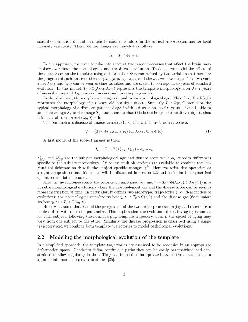
In our approach, we want to take into account two major processes that affect the brain mor-phology over time: the normal aging and the disease evolution. To do so, we model the effects ofthese processes on the template using a deformation Φ parametrized by two variables that measurethe progress of each process: the morphological age λMA and the disease score λDS . The two vari-ables λMA and λDS can be seen as time variables and are scaled to correspond to years of standardevolution. In this model, T0 ◦ Φ(λMA, λDS) represents the template morphology after λMA yearsof normal aging and λDS years of normalized disease progression.

In the ideal case, the morphological age is equal to the chronological age. Therefore, T0 ◦Φ(t, 0)represents the morphology of a t years old healthy subject. Similarly T0 ◦ Φ(t, t′) would be thetypical morphology of a diseased patient of age t with a disease onset of t′ years. If one is able toassociate an age λ0 to the image T0, and assumes that this is the image of a healthy subject, thenit is natural to enforce Φ(λ0, 0) = Id.

The parametric subspace of images generated like this will be used as a reference:

T = {T0 ◦ Φ(λMA, λDS) for λMA, λDS ∈ R} (1)

A first model of the subject images is then:

Ik = T0 ◦ Φ(λkMA, λkDS) ◦ φk + εk

λkMA and λkDS are the subject morphological age and disease score while φk encodes differencesspecific to the subject morphology. Of course multiple options are available to combine the lon-gitudinal deformation Φ with the subject specific changes φk. Here we write this operation asa right-composition but this choice will be discussed in section 2.2 and a similar but symetricaloperation will later be used.

Also, in the reference space, trajectories parametrized by time t 7→ T0 ◦Φ(λMA(t), λDS(t)) givepossible morphological evolutions where the morphological age and the disease score can be seen asreparametrization of time. In particular, it defines two archetypal trajectories (i.e. ideal models ofevolution): the normal aging template trajectory t 7→ T0 ◦ Φ(t, 0) and the disease specific templatetrajectory t 7→ T0 ◦ Φ(λ0, t).

Here, we assume that each of the progression of the two major processes (aging and disease) canbe described with only one parameter. This implies that the evolution of healthy aging is similarfor each subject, following the normal aging template trajectory, even if the speed of aging mayvary from one subject to the other. Similarly the disease progression is described using a singletrajectory and we combine both template trajectories to model pathological evolutions.

2.2 Modeling the morphological evolution of the templateIn a simplified approach, the template trajectories are assumed to be geodesics in an appropriatedeformation space. Geodesics define continuous paths that can be easily parametrized and con-strained to allow regularity in time. They can be used to interpolate between two anatomies or toapproximate more complex trajectories [25].

5

In this paper, we use the stationary velocity field (SVF) framework [26] for its ability to describecomplex and realistic diffeomorphic (smooth and invertible) brain deformations in a straightforwardmanner [27]. In this framework, the observed anatomical changes are encoded by diffeomorphismswhich are parametrized with the flow of SVFs. Within this setting, the metric between deformationsis not chosen a priori even if we need a regularization criterion for the registration. To compute adeformation φ we integrate trajectories along the vector field v for a unit of time.

φ(x) = φ1(x) =

∫ 1

0

v(φt(x))dt with φ0 = Id

This relationship is denoted as the group exponential map φ = Exp(v).By writing Φ(λMA, λDS) = Exp(λMAvA +λDSvD), we propose a linear model in the SVF space

(i.e. the space of the parameter of the deformations) parametrized by two SVFs vA and vD. Inparticular, the two template trajectories are then separately parametrized: vA controls the normalaging template trajectory and vD the disease specific template trajectory.

Besides, for each subject, the processes are meant to be intertwined and it can be modeled indifferent ways depending on the parametrization of the trajectories, for instance a right or a leftcomposition. The proposed linear combination of the parameters provides us a middle ground.Indeed in the SVF setting, the relationship between composition and the linear combination ofSVFs is given by the Baker-Campbell-Hausdorff formula [28] and the linear combination of theSVFs is equivalent to alternate between right and left composition with infinitesimal steps.

To sum up, the longitudinal deformation Φ modeling the effects of the aging and the disease ona reference morphology T0 is parametrized by two SVFs: vA and vD. This ideal model generates asurface T of possible images describing the evolution of the template morphology:

T = {T0 ◦ Exp(λMAvA + λDSvD) for λMA, λDS ∈ R} (2)

2.3 Individual morphological variability and generative modelAn individual image is modeled as follows:

Ik = T0 ◦ Exp((λkMA − λ0)vA + λkDSvD) ◦ φk + εk (3)

where the choice of the intensity noise εk is implicitly related to the registration similarity metric.To specify the constraint on φk, we define a subject specific residual SVF wk

r (r stands for residual)such that:

Exp((λkMA − λ0)vA + λkDSvD) ◦ φk = Exp((λkMA − λ0)vA + λkDSvD + wkr )

In this formula, Exp(wkr ) is approximatively equal to φk given the first order of the BCH equation

between composition and linear combination of SVFs. Moreover, we wish to have the subjectspecific deformation to encode what cannot be described using the template trajectories. That iswhy we impose wk

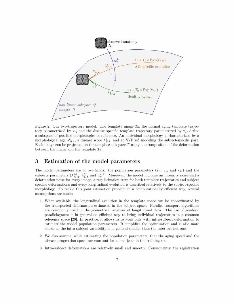
r to be orthogonal to both vA and vD.As we can see in Figure 2, the model parametrized by vA and vD allows us to characterize the

subject morphology with two scalar variables, the morphological age λkMA and the disease score λkDS ,and a SVF wk

r for the subject-specific part. The orthogonality constraint makes the description ofthe subject uniquely defined. We denote by wk the subject-to-template deformation SVF:

wk = (λkMA − λ0)vA + λkDSvD + wkr (4)

6

vD

vA

λkDS

λkMA

wkr

non linear subspace ofimages T

t 7→ T0 ◦ Exp(tvD)

t 7→ T0 ◦ Exp(tvA)

AD-specific evolution

Healthy aging

observed anatomyIk

Figure 2: Our two-trajectory model. The template image T0, the normal aging template trajec-tory parametrized by vA and the disease specific template trajectory parametrized by vD definea subspace of possible morphologies of reference. An individual morphology is characterized by amorphological age λkMA, a disease score λkDS , and an SVF wk

r modeling the subject-specific part.Each image can be projected on the template subspace T using a decomposition of the deformationbetween the image and the template T0.

3 Estimation of the model parametersThe model parameters are of two kinds: the population parameters (T0, vA and vD) and thesubjects parameters (λk,iMA, λ

k,iDS and wk,i

r ). Moreover, the model includes an intensity noise and adeformation noise for every image, a regularization term for both template trajectories and subjectspecific deformations and every longitudinal evolution is described relatively to the subject-specificmorphology. To tackle this joint estimation problem in a computationally efficient way, severalassumptions are made:

1. When available, the longitudinal evolution in the template space can be approximated bythe transported deformation estimated in the subject space. Parallel transport algorithmsare commonly used in the geometrical analysis of longitudinal data. The use of geodesicparallelograms is in general an efficient way to bring individual trajectories in a commonreference space [29]. In practice, it allows us to work only with intra-subject deformation toestimate the model population parameters. It simplifies the optimisation and is also morestable as the intra-subject variability is in general smaller than the inter-subject one.

2. We also assume, while estimating the population parameters, that the aging speed and thedisease progression speed are constant for all subjects in the training set.

3. Intra-subject deformations are relatively small and smooth. Consequently, the registration

7

regularisation has less impact on the estimated deformation. It allows us to estimate theselongitudinal evolutions independently of the population model.

These assumptions allow us to efficiently decompose the problem of the parameter estimation.First, subjects with longitudinal data are processed independently and the intra-subject evolutionsare modeled in the subject space. Then the population parameters (T0, vA and vD) are estimatedusing only intra-subject longitudinal evolutions.. Finally, the subject parameters are estimated foreach subject.

3.1 Estimation of the template trajectories vA and vD in a given templatespace

In this section we suppose that we know T0 and that we can compute the subject-to-templatedeformation wk for a reference time point. We also consider that we have longitudinal data forevery subject.

First we address the inverse problem of estimating the intra-subject evolution parameters withthe framework proposed by Hadj-Hamou et al. [30]. Images are preprocessed, rigidly aligned to theMNI-152 template and then longitudinally registered. Intra-subject deformations between follow-upimages Ik,i and the baseline image Ik,0 are computed using non-linear registration. The resultingintra-subject model in the subject space is estimated using an ordinary least square regression in thetangent space of SVFs. It is equivalent to the assumption that the deformation noises are centered,uncorrelated and have equal variance in the space of SVFs.

Then for a given template T0 and subject-to-template deformation wk, the intra-subject modelcan be transported using parallel transport in the template space to get vk. This deformation canbe decomposed along the template trajectories giving a morphological aging rate (noted skMA), adisease progression rate (noted skDS) and an orthogonal component (noted vkr ):

vk = skMAvA + skDSvD + vkr

The estimation is done on two groups of subjects: Gh with the healthy subjects and Gad withpatients diagnosed with AD. We assume that each healthy subject of Gh is aging at normal speedskMA = 1,∀k ∈ Gh and does not have any evolution toward the disease skDS = 0,∀k ∈ Gh. Similarly,each patient of Gad has a normal morphological aging rate skMA = 1,∀k ∈ Gad and a constant unitdisease progression rate skDS = 1,∀k ∈ Gad. Finally the subject specific components are assumed tobe centered, uncorrelated and to have a fixed variance. The maximum likelihood problem writes:

minvA,vD

∑k∈Gh

‖vk − vA‖2 +∑

k∈Gad

‖vk − vA − vD‖2 (5)

The solution of the optimization problem is explicit:

v̂A =1

|Gh|∑k∈Gh

vk (6)

v̂D =

(1

|Gad|∑

k∈Gad

vk

)− v̂A (7)

We should however note that ‖v̂A‖ (resp. ‖v̂D‖) is a biased estimator of ‖vA‖ (resp. ‖vD‖). Wedetail the bias estimation in the Appendix 8.2.

8

3.2 Estimation of the template morphology T0

The population specific template morphology is computed using the algorithm proposed by Gui-mond et al. [31] by alternating the registration of subject images to the template and the recom-putation of the template intensity. However, in our approach, the subject image should not beregistered to T0 directly but to its projection on the template space.

To tackle this problem, we propose an iterative procedure where we iteratively register the imageto its current projection on the reference space. Algorithm 1 details the procedure with simplifiednotations in the general case where w parametrizes the deformation between the image I and T , thereference linear subspace of SVF is denoted T and w is decomposed accordingly w = wt +wr withwt ∈ T , wr ∈ T ⊥. The registration regularization should only be applied to the residual part wr. Inthe context of the LCC-demons registration algorithm, it boils down to the following minimizationproblem (see [27]):

minwt∈T ,wr∈T ⊥,w′

Sim(I, T,Exp(wt + wr)) + Dist(wr, w′) + Reg(w′)

The idea is to alternate between the optimization and the projection on the constraints.Data: an image I, a template image T and linear space of SVF TResult: two SVFs: wt ∈ T , wr ∈ T ⊥wt = 0 ;repeat

wr = registration(T ◦ Exp(wt), I) ;wt = wt + projT (wr);

until wr ⊥ T ;Algorithm 1: Iterative registration algorithm

As we do not have any theoretical guarantee on the convergence of the algorithm, the stabilityand the convergence will be evaluated empirically.

As the template estimation also involves iterative search, we can combine both algorithms fora faster optimisation. The projection coordinates are kept from one iteration to the next and theimages are registered to their estimated projections in the template space. The deformation updateu is then computed and finally the new atlas image T and the estimated projections are updated(see Algorithm 2).

Data: a set of images (Ik) and a linear space of SVF TResult: a template image T , a set of pairs of SVFs (wk

t , wkr )

wkt = 0 for all k;

initialize T ;repeat

wkr = registration(T ◦ Exp(wk

t ), Ik) ;u = mean(wk

r ) ;T = mean(Ik ◦ Exp(−wk

r + u)) ;wk

t = wkt + projT (wk

r − u) ;until convergence;

Algorithm 2: Iterative template space estimation algorithmIt is even possible to go further and to update the SVFs parametrizing T at each iteration. In

this work, we do it and transport the subject intra-subject models to the template space and updatethe template trajectories at each iteration. T is initialized using the MNI-152 template and the

9

convergence is manually assessed comparing the template for successive iterations. At convergence,we then have the template image T0 and both template trajectories vA and vD.

3.3 Estimation of the subject parametersIf the population parameters are set, the estimation of the individual parameters for a new subjectis relatively simple. The deformation wk is computed by registration between a subject image andthe template using Algorithm 1 and then decomposed linearly wk = (λkMA − λ0)vA + λkDSvD +wk

r

by solving the following linear system:

wk · vA = ‖vA‖2(λkMA − λ0) + vD · vAλkDS (8)

wk · vD = vD · vA(λkMA − λ0) + ‖vD‖2λkDS (9)

In practice, the estimation is not exact because we work the noisy estimator v̂A and v̂D. Thelinear decomposition can also be computed locally or using any voxel weighting by modifying thescalar product. When longitudinal data is available, this estimation is independently done for eachtime point.

4 Results

4.1 Experiments with synthetic dataWe first evaluate our approach using synthetic data in order to assess the accuracy and the re-producibility of the biomarkers estimation. Realistic longitudinal MRIs are simulated using thesoftware proposed by Khanal et al. [32]. It relies on a biophysical model of brain deformation andcan be used to simulate longitudinal evolutions with specific atrophy patterns. In this context, localatrophy is measured by the divergence of the stationary velocity field.

4.1.1 Simulated dataset

In this controlled experiments we choose to simulate two populations that are characterized by theiratrophy patterns and that respectively emulate healthy controls and diseased patients. Atrophyof the aging brain and the effect of AD have been extensively studied [33] and the atrophy mea-surements may vary depending on the methodology and the population studied. In this work, wechoose to prescribe piecewise-constant atrophy map with constant value in brain areas delimitedby the segmentation software FreeSurfer. The atrophy value of a region is sampled around a fixedpopulation mean with an additive Gaussian noise of relative standard deviation of 5% for everysubject. The healthy population is designed to have a slight atrophy in the whole brain while thediseased patients have a stronger atrophy especially in the hippocampal areas and the temporalpoles. The means are chosen to give the order of magnitude of a one year evolution accordingly towhat was reported in Fjell et al. [34] for healthy aging and in Carmichael et al. [35] with an addi-tional scaling for the pathological evolution. We detail the exact regional specifications in table 2in the appendix (see 8.1).

Structural MRIs of 40 healthy subjects from the ADNI database are taken as input to thesimulations. For every subject, deformations are simulated for both the pathological and the healthysettings. The deformation is then extrapolated 5 times before being applied to the original image.We then have two matched populations of 40 pairs of images.

10

4.1.2 Model estimation

Individual longitudinal deformations are computed using registration and the reference anatomyand the template trajectories are built using our framework. The divergence fields associated withthese template trajectories can be compared to the prescribed atrophy (see Figure 3). The atrophyground truth is computed using the estimated template anatomy as the anatomical variability isnot explicitly model.

The estimated atrophy patterns are smoothed versions of the simulated ground truth. This effectwas already observed [32]. First of all, the registration algorithm is unaware of the underlyingsimulation model and is unable to localize the atrophy in homogeneous areas. Moreover, thespatial regularization of the registration and the parametrisation using SVFs are also smoothingthe estimated atrophy patterns. It is particularly visible in small (hippocampus) or thin regions(cortex). This results in a consistent bias when the atrophy measurements are integrated over theregions (see Figure 15 in appendix). Indeed, the local atrophy is affected by neighboring regionsevolving in the opposite direction (the ventricles or the CSF for example). However, we can see thatthe ratio between the pathological and healthy cases is conserved in every region. It was alreadynoted that quantitative estimation using registration can be biased but more reproducible [36, 37].We want to see how these limitations of the deformation based morphometry are translated intothe proposed age and disease progression markers.

4.1.3 Imaging biomarkers estimation

The morphological age and the disease score were computed for each image. By construction thereis no difference at t=0 (exactly the same images in the two groups). We can compare the simulateddifferences at t=5 or the evolution of the cross-sectional assessments for each subject (see Figure 4).

In this experiment, the initial anatomical variability is really important, indeed the standarddeviation at t=0 is equal to 48 years for MA(0) and 24 years for DS(0). At t=5, a difference isvisible for the disease score but it is still diluted in the inter-subject variability. It is also possibleto extrapolate the evolution to determine how many years of evolution are needed in order to geta significant difference between the healthy and the disease groups. Here, the statistical analysisgives that, for a significativity level of 0.05, the disease score would be significantly discriminantafter 13 years of evolution. It is done for synthetic data but it highlights the slowness of the diseaseand the interest in modeling to be able to extrapolate the evolutions.

Looking at the evolution of these cross-sectional biomarkers, we see that the measure is rela-tively stable despite the relatively large inter-subject variability. It seems that doing the measureat two different time points gives a good estimate of the longitudinal evolution. Even if the sim-ulation images was not done independently of our generative model, it is able to explained mostof the simulated changes. In practice the estimations are a bit biased, for example the increase ofmorphological age ∆MA = MA(5)−MA(0) is expected to be equal to 5 for both populations whilethe the mean of the estimation is equal to 3.92 for the healthy group and to 3.57 for the diseasedgroup. But more importantly, the standard deviation is really small in comparison to the standarddeviation of the cross-sectional measurement (σ∆MA = 1.13 while σMA(0) = 47.8). For the changeof disease score ∆DS, the mean is close to 0 for the healthy group and close to 5 for the diseasedgroup. The variance is also very small with respect to the cross-sectional one. In particular thedifference between healthy and diseased subjects is clearly observed for the longitudinal evolution:the difference between the means is equal to 3.2 standard deviation for ∆DS.

In a clinical context where longitudinal data is not always available, it is important to get as

11

(a) Healthy evolution

(b) Pathological evolution

relative volume change (year−1)

Figure 3: Simulated and estimated atrophy patterns in the template space. Top row: mean in thetemplate space of the prescribed atrophy maps. Bottom row: atrophy maps estimated from thesimulated images. Left: healthy simulations. Right: pathological simulations. The estimation issmoother but even local pattern such as in the one in hippocampal area are captured and globallythe simulated and estimated maps are qualitatively similar.

12

MA(t=5)

DS(t=5)

75

50

25

0

25

50

75

100

Cross-sectional markersHealthyDiseased

MA

DS*

4

2

0

2

4

6

8

10 Longitudinal evolutionsHealthyDiseased

Figure 4: Evolution of the imaging biomarkers estimated on simulated data. MA=morphologicalage, DS=disease score. The longitudinal evolutions ∆MA and ∆DS are the differences between thetwo cross-sectional assessments i.e. ∆MA = MA(5) - MA(0). The star indicates that the differencebetween the healthy and the diseased subjects is significant (p-value < 0.05) for an unpaired t-test.By construction there is no difference between the two populations at baseline. The changes aregenerally underestimated when using the difference between the two cross-sectional measurementsbut the longitudinal evolutions show the stability of the estimation despite a strong variabilityinter-subject.

much information as possible from every cross-sectional measurement. We see here that the markersmay not be the best to separate the two populations but the cross-sectional measurement gives arelatively stable assessment and their evolutions are strongly associated with the clinical diagnosis.

4.2 Experiments with real dataLongitudinal T1 sequences were obtained from the Alzheimer’s Disease National Initiative (ADNI).Subjects are classified according to the evolution of their cognitive diagnosis. Three diagnoses arepossible at each time point: normal, mild cognitive impairment (MCI) and Alzheimer’s disease.The normal diagnosis and the MCI stable group are also sub-classified using the beta-amyloid 1-42biomarker that has been shown to be related to prodromal condition. We then have 6 distinctsub-groups: CN- (cognitively normal with negative Aβ), CN+ (cognitively normal with positiveAβ), MCIs- (MCI stable during the study time-window with negative Aβ), MCIs+, MCIc (MCIconverter to AD) and AD (diagnosed with Alzheimer’s disease starting from the beginning). Thetable 1 sums up the demographic description of the population. We can notice that the group sizesare a bit unbalanced as we divided the cognitively normal group (272 subjects in total) in threebut otherwise the groups are well matched in age with slightly uneven gender distributions.

We estimate our template morphology and the template trajectories on a subset of subjects. Inorder to form this training set, we randomly selected 30 subjects from the CN- group and 30 fromthe AD group. To reduce the variability associated with the estimation of the model, these subjectswere selected among the ones with strictly more than one followup acquisitions. In the following we

13

group CN- CN+ MCIs- MCIs+ MCIc ADNumber of subjects 108 69 96 120 228 203Age at baseline 73.4 (5.6) 74.5 (6.5) 71.1 (7.7) 73.5 (6.6) 73.8 (7.1) 74.5 (7.7)Gender (female) 47.2% 56.5% 47.9% 37.5% 41.7% 48.3%Education (years) 16.4 (2.6) 16.2 (2.7) 16.2 (2.8) 16.4 (2.7) 16.0 (2.9) 15.0 (2.9)ADAS13 at baseline 9.0 (4.0) 8.6 (5.0) 12.0 (4.9) 14.0 (5.4) 19.9 (6.7) 31.4 (7.3)

Table 1: Socio-demographic and clinical information of the study cohort. Standard deviations areshown in brackets.

distinguish between the training set of 30+30 subjects used to build the model and the remainingtesting set (with in particular 78 CN- subjects and 173 AD subjects).

4.2.1 Estimation of the normal aging and the disease-specific template trajectories

The template anatomy is an average of the healthy subjects anatomies, so its age corresponds to themean group age λ0 = 73.46 y.o. The result of the estimation is shown in Figure 5. The estimatednormal aging template trajectory is characterized mainly by ventricular expansion caused by theatrophy of the surrounding regions. Disease specific changes are widespread in the brain with astrong emphasis on the temporal areas.

Atrophy patterns can be measured by the divergence of the velocity field. We see in Figure 6 thatthey are similar to what was already observed in the past for healthy and the diseased subjects [36].The precise localization of the atrophy is always difficult with a morphometrical approach but wesee for the healthy group a well spread and relatively small atrophy while the additional diseasespecific atrophy is particularly strong in the temporal area. It also seems that the remaining atrophyin the rest of the brain, is mainly located near the cortical surface.

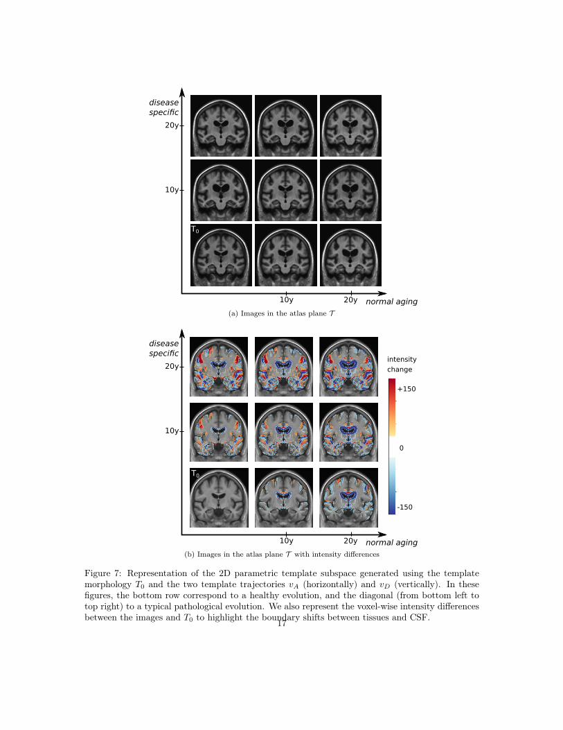
The generative model can be used to get images in the reference template plane to visualize themodeled morphologies. Figure 7 shows the evolution of the template morphology in the two maindirections. It shows the evolution over 20 years. The difference of intensity overlay is used to showsthe changes of tissue boundaries. The global atrophy and the expansion of the ventricles is clearlyvisible for the aging evolution. The pathological changes are associated with smaller structures butthe shrinking of the hippocampi, the atrophy of the temporal lobes and also the widening of thesulci (related to the cortical thickening) are visible.

4.2.2 Intra-subject variability of our progression markers

In Lorenzi et al. [24], a morphological age similar to our measure was shown to be correlated withthe chronological age and also that advanced AD stages were associated with “morphologicallyolder” brains. To go further, we want to show that our proposed model represents also the aging atthe individual level. For multiple acquisitions of a same subject, an aging measurement is expectedto increase smoothly with time. And if the subject is healthy, we can expect a linear increase witha slope of 1. We should also see the increase of disease score for the patients while this marker staysstable and close to 0 for the healthy subjects. These hypotheses are evaluated using data from theADNI datasets.

The morphological age and the disease score are computed for each subject at each time point.Figure 8 shows the evolution of these cross-sectional measurements. First, at the population level,

14

(a) Normal aging template trajectory (b) Disease specific template trajectory

(mm · year−1)

Figure 5: Template image and SVFs parametrizing the two template trajectories SVFs. Left:normal aging trajectory vA showing a ventricular expansion related to a global atrophy. Right:disease specific trajectory vD showing specific patterns, especially in the temporal lobes around thehippocampi areas. The color encodes the amplitude of the velocity at each position.

subjects are generally associated with a morphological age similar to their chronological age eventhough its variability is quite high. Second, for each subject, the evolution is mostly linear andthe morphological age steadily increases. Third, the disease score also steadily increases for eachsubject. Finally, we can also note that the AD subjects look older, age faster and have a higherdisease score than the healthy ones.

A linear random effects model can help us to quantify these observations. The model is fitted, forboth morphological age and disease score, with fixed effects on age and sex and a random interceptand slope for each subject. The focus is set on the analysis of the regression for the CN and the ADgroups. For each coefficient of the regression we also show the standard deviation of the estimation.

The model is first fitted to the morphological age measures in the CN group. It gives a coefficientof 0.26 ± 0.11 for the fixed effect of age while the mean subject slope is 0.10 ± 0.02. Both aresignificantly positive. In comparison to the same model without the random slope the relativeimprovement brought by the intra-subject linear evolution is significant by a large margin (p-value inferior to 10−6 for the likelihood ratio test). The regression has also a positive (but notsignificatively) coefficient for male subjects (1.81±1.2) meaning that male morphologies looks older(similar to a 7 years shift).Concerning the disease score, we also observe a relatively good fit ofthe linear model. The evolution is generally slower with 0.12 ± 0.1 for the fixed effect of age and0.12± 0.01 for the mean individual slope.

For the AD group, the linear model is also well adapted (p-values inferior to 10−6 for the

15

(a) Atrophy along the normal aging template trajectory

(b) Atrophy along the disease specific template trajectory

relative volume change (year−1)

Figure 6: Atrophy measured by the divergence of the SVFs parametrizing the two template trajec-tories.

16

normal aging

disease specific

10y

10y

20y

20y

T0

(a) Images in the atlas plane T

T0

normal aging

disease specific

10y

10y

20y

20y

intensity

change

+150

0

-150

(b) Images in the atlas plane T with intensity differences

Figure 7: Representation of the 2D parametric template subspace generated using the templatemorphology T0 and the two template trajectories vA (horizontally) and vD (vertically). In thesefigures, the bottom row correspond to a healthy evolution, and the diagonal (from bottom left totop right) to a typical pathological evolution. We also represent the voxel-wise intensity differencesbetween the images and T0 to highlight the boundary shifts between tissues and CSF.

17

likelihood ratio test). The main remark is probably that the intra-subject slopes are in average moreimportant than for healthy subjects (around 0.52± 0.06 for the morphological age and 0.71± 0.05for the disease score) while the fixed effect related to age of 0.23± 0.07 (for the morphological age)and 0.14± 0.04 (for the disease score) are more similar to the one observed previously.

60 70 80 90chronological age

60

65

70

75

80

85

90

95

morp

holo

gic

al ag

e

CN- (train)

AD (train)

60 70 80 90chronological age

10

5

0

5

10

15

dis

ease

sco

re

CN- (train)

AD (train)

Figure 8: Evolution of cross-sectional markers for every subject of the two training sets. [Left]chronological age, the dashed line corresponds to the expected evolution of healthy subjects i.e. themorphological age is equal to the chronological age. [Right] disease score, the dashed line is theexpected pathological evolution.

4.2.3 Cross-sectional discriminating power

We saw that the two markers are able to represent realistic evolutions of healthy and diseasedsubjects. We want to study their relation to the disease progression. We start with a simplediscriminant analysis using only the first image available for each subject.Figure 9 shows the dis-tribution of the estimations for each group. We see a gradual increase of both markers towardsmore advanced disease states. Significant differences in morphological age and in disease score areobserved between the control group CN-(train) and both the MCIc and AD groups. Both mark-ers show the same trend, but marginal pattern can be distinguished. For instance, the differencebetween the MCI stable and the MCI converters is stronger for the morphological age while thedisease score differentiate more between the MCIs- and the MCIs+. As such, the morphologicalage is more associated with the general cognitive degradation while the disease score seems morecorrelated with more AD-specific biomarkers.

We also perform a simple linear classification task between the MCIs and MCIc groups usingthis two cross-sectional markers. A SVM linear classifier is fitted to the full data-set to perform thebinary classification using the scikit-learn python library. The error penalty weights are adjustedbetween the two classes to balance the trade-off between true positive rate (correct classification ofAD subjects) and false positive rate (incorrect classification of healthy ones). The mean classifica-tion accuracy using a 10-folds cross-validation scheme is equal to 0.59. Of course we do not reachthe performance of state-of-the-art dedicated algorithm (the same classifier using the normalised

18

CN-

CN+

MCIs-

MCIs+

MCIc AD20

10

0

10

20

30

40 Morphological agep<0.01

CN-

CN+

MCIs-

MCIs+

MCIc AD10

5

0

5

10

15

20 Disease scorep=0.05

Figure 9: Box-plot of the group-wise markers estimated for the clinical groups. Stars below thename of the group indicate a significant difference to the CN- group for a t-test at the level 0.05.Both markers gradually increase towards more advanced disease states.

volume of the hippocampi has a 0.67 accuracy) but it allows us to see how both markers are as-sociated with the diagnosis. Moreover this discriminative approach could be extended by usinginformation in a subset of targeted areas.

Here, the linear decision function is equivalent to the projection on the SVF vA − 0.003vD, sothe differences between MCIs and MCIc subjects is, in our model, only associated with the agingtrajectory. The disease specific changes do not seem to have an impact before the conversion. We cancompare this to the similar experiment between CN and AD where the linear classifier correspondsto the projection on vA + 0.49vD so approximately (vbn + vad)/2, i.e. the mean evolution of thewhole population.

4.2.4 Regional analysis of the progression

In the context of Alzheimer’s disease, most of the morphological changes are known to be locatedin the temporal lobe. Using the AAL atlas [38], we segment the temporal lobe of our templateanatomy. The mask is then used to compute the regional morphological age and disease score foreach subject. Results are shown in Figure 10.

The region is not adapted to the morphological age model. Indeed, for a healthy subjectthe deformations in this area are really small. However the choice of a disease-adapted regionis improving the performance of the disease score. It is now able to capture early specific changesand the difference between CN- and CN+ is significant.

4.2.5 Longitudinal evolution of the markers

To explore more in details the longitudinal evolution of these markers, a linear model is fitted to theindividual evolutions. The intercept can be interesting as it aggregates the measure at every timepoint and helps reduce the noise but more importantly the slope can be very informative. Resultsare shown in Figure 11 for the whole brain markers.

A progressive evolution, from CN- to AD, is visible for the morphological age with subjectsevolving faster and faster. It is a bit more complex for the disease score. The evolution is almost

19

CN-

CN+

MCIs-

MCIs+

MCIc

AD30

20

10

0

10

20

30

40

50 Morphological age (temporal area)

p>0.05 p<0.01

CN-

CN+ MCIs-

MCIs+

MCIc AD30

20

10

0

10

20

30 Disease score (temporal area)

p=0.03 p=0.05

Figure 10: Box-plot of the markers estimated in the temporal lobes. Stars below the name of thegroup indicate a significant difference to the CN- reference for a t-test at the level 0.05. The areaknown to be related to the AD makes the disease score estimation less sensitive to the overall noise.

negligible for CN- and MCIs- and relatively slow for CN+ and MCIs+ while the changes are clearlyvisible for MCIc and AD. Significant differences are visible between healthy subjects (CN-) andMCIc or AD subjects or even between MCI stable and MCI converter subjects, but also betweenMCIs- and MCIs+ (or more generally between subjects with negative amyloid or positive amyloidmarker). It means that we are able to capture the global progression of the disease. The changesare stronger for diagnosed patients but similar patterns of evolution are observed in the early stageof the disease. It is a good sign to indicate that the marker may be able to identify precursor signof the disease, however it is difficult to draw definitive conclusions because of the difference is smallrelatively to the variability and the statistical tests are not corrected for multiple comparisons. Asignificant difference is also observable between the CN- and CN+ group for the temporal diseasescore slope.

CN-

CN+

MCIs-

MCIs+ MCIc AD4

2

0

2

4

6 Morphological age slope

p<0.01

CN-

CN+

MCIs-

MCIs+ MCIc AD3

2

1

0

1

2

3

4

5 Disease score slope

p<0.01p<0.01

Figure 11: Box-plot of the rate of evolution of the markers computed using individual linear regres-sions. Stars indicate a significant difference to the CN- reference for a t-test at the level 0.05. Toprow shows the results for the whole brain while the bottom row shows the result for the temporallobe only. A gradation is visible from the healthy to the diseased subjects.

20

The disease score evolution is close to zero for the healthy subject and close to one for thepathological one but more generally, the slopes are in average smaller than their expected values.For example the average disease score evolution in the AD group is equal to 0.82 and this divergenceis particularly important for the morphological age slope of the CN- group that is only equal to 0.33(instead of 1). This bias was already observer previously and be in part explained by the estimationprocedure: the norm of the SVF parametrizing the template trajectory and by consequence thenormalization are known to be biased (see 8.2).

4.3 Generating diagnosis driven morphological evolutionOne of the main advantage of our model is its ability to be generative. From a couple (morphologicalage, disease score) we are able to generate a corresponding morphology. It is also possible to deforma specific subject anatomy in the directions defined by the template trajectories. In this section, themodel is used to to generate plausible morphological evolutions of a subject, for several diagnosiscondition, and compare them to the observed one.

4.3.1 Modeling the group evolution

To predict a subject evolution it is natural to look at subjects that are similar. This similarity willbe based on the morphological age and the disease score and will be restricted to subjects of thesame clinical condition.

In practice, each subject is associated with a couple (position, speed) in the parameter plane,then, for each group, a vector field is regressed using a kernel ridge regression to estimate thelocal speed at every point. It uses a RBF kernel with a spatial scale set to 10 years (for both themorphological age and the disease score axis) in order to get large scale patterns despite the highinter-subject variability. The regularization weight, which does not seem to have a large effect onthe result, is set to 1. Results are presented in Figure 12 for the CN (i.e CN-, CN+ together),MCIs, MCIc and AD groups. The figure is centered on the data and the extrapolation can be reallyunreliable.

Differences in amplitude, i.e. speed of evolution, and orientation are clearly visible betweenthe groups and echo the results about the linear regression coefficients in the previous section. Inparticular we see a progressive amplitude increase from the CN group to the AD group.

These diagrams also help to describe the variability within a same clinical group. For theCN group we can distinguish between the low disease score and low morphological age area (inthe bottom left) where in average the changes are negligible, and the rest where there is a slowhorizontal evolution. It suggests that the healthier and younger subjects are morphologically stableand do not show the same visible aging process. The MCI stable evolution is relatively uniform andin average a bit stronger but overall really similar to the CN one. The MCI converters however showa stronger and more vertical evolution. The angle of the average vector is equal to 38◦ while it wasequal 30◦ (resp. 31◦) for the MCIs (resp. CN) group. We should also note that subjects with highmorphological age and low disease score (bottom right) seem to follow a different, more horizontalevolution. It means fast morphological aging but less important disease specific changes. The ADgroup confirms this trend and in fact MCIc and AD look very similar. The mean evolution is strongand more vertical (angle equal to 46◦ for the average). A main evolution is visible from bottom leftto top right with a sightly more horizontal part in the middle giving this global tangent-like aspect.Beside, a horizontal evolution, similar to what was observed for the MCIc model, is also visible in

21

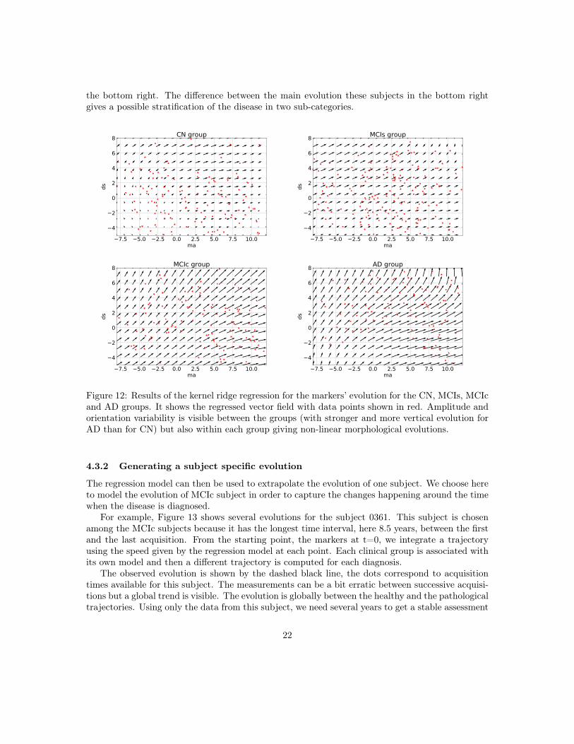
the bottom right. The difference between the main evolution these subjects in the bottom rightgives a possible stratification of the disease in two sub-categories.

7.5 5.0 2.5 0.0 2.5 5.0 7.5 10.0ma

4

2

0

2

4

6

8

ds

CN group

7.5 5.0 2.5 0.0 2.5 5.0 7.5 10.0ma

4

2

0

2

4

6

8

ds

MCIs group

7.5 5.0 2.5 0.0 2.5 5.0 7.5 10.0ma

4

2

0

2

4

6

8

ds

MCIc group

7.5 5.0 2.5 0.0 2.5 5.0 7.5 10.0ma

4

2

0

2

4

6

8

ds

AD group

Figure 12: Results of the kernel ridge regression for the markers’ evolution for the CN, MCIs, MCIcand AD groups. It shows the regressed vector field with data points shown in red. Amplitude andorientation variability is visible between the groups (with stronger and more vertical evolution forAD than for CN) but also within each group giving non-linear morphological evolutions.

4.3.2 Generating a subject specific evolution

The regression model can then be used to extrapolate the evolution of one subject. We choose hereto model the evolution of MCIc subject in order to capture the changes happening around the timewhen the disease is diagnosed.

For example, Figure 13 shows several evolutions for the subject 0361. This subject is chosenamong the MCIc subjects because it has the longest time interval, here 8.5 years, between the firstand the last acquisition. From the starting point, the markers at t=0, we integrate a trajectoryusing the speed given by the regression model at each point. Each clinical group is associated withits own model and then a different trajectory is computed for each diagnosis.

The observed evolution is shown by the dashed black line, the dots correspond to acquisitiontimes available for this subject. The measurements can be a bit erratic between successive acquisi-tions but a global trend is visible. The evolution is globally between the healthy and the pathologicaltrajectories. Using only the data from this subject, we need several years to get a stable assessment

22

4 2 0 2 4 6morphological age

4

6

8

10

12

dise

ase

scor

e

I0

Evolution scenarii for subject 0361observed evolutionsimulated CNsimulated MCIssimulated MCIcsimulated AD

Figure 13: Real and generated marker evolutions for the subject 0361. The observed evolutionappear to be between the CN and the AD evolution and close to the MCIc one.

of the morphological evolution while the models regressed from the population are able to simulaterealistic changes in the medium to long term.

We see that the observation is more similar to the MCIs or the MCIc model. It highlights thatusing additional clinical condition improves the model as our cross-sectional imaging biomarkers donot fully capture the status of the subject relatively to the disease and are not designed to replacea diagnosis or any clinical information.

These markers changes can be directly translated in brain images to visualize the morphologicalevolution. Figure 14 shows the results for the end point of the trajectories. Results are shown forthe CN and AD models only. We have seen that the estimation of the markers was biased. For boththe synthetic dataset and the training samples the measured changes only correspond to 80% of theexpected value. In order to get images that correspond to the desired changes we then multiply thedeformations by 1.25. Images are generated by deforming the baseline image using the simulateddeformation transported in the subject space.

The cortical atrophy in particular in the temporal lobe is clearly visible in the real image and toa lesser extent in the AD simulation. The expansion of the ventricles is also visible in every image,but again even in the AD simulation the volume change is inferior to the observation. It seems thatwe only partially capture the changes related to AD. Other aspects of the evolution are hard toquantify and often poorly documented. For example the evolution of the shape of the ventricles isdifferent in the three images. It may be related to different spatial distribution of the degenerationin the brain and inherent mechanical constraints. We also observe a global motion of loweringof the temporal lobe and a local rotation in the image for the real case and the AD simulation.Overall, the morphological changes simulated looks realistic, even if they do not matches perfectlythe observed changes because the model is generic and really simple. It gives a range of possibleevolution that can be further exploited to see what is expected or not.

23

baseline simulatedCN

simulatedAD

realt=8.5y

B

C

A

Figure 14: Evolution of the subject 0361 over more 8.5 years. The subject was diagnosed MCI (for5y) then AD. From left to right: (1) real image at baseline, (2) simulated image from the baselineimage using the healthy (CN) evolution, (3) using the pathological (AD) evolution, (4) real imageat t=8.5y. The second row zooms in the most interesting areas between the ventricle (A), thelateral sulcus (B) and the hippocampus area (C). Even if the simulated changes do not match thefull extend of the real case, the atrophy is visible in the sulcus and the hippocampus and there isa difference in shape and size of the ventricles.

5 Contributions and limitationsIn this work, we proposed to describe the evolution of elderly patients using two trajectories thatmodel the morphological evolution of the brain for healthy or pathological cases. Biological (orhere morphological) age estimates were proven to be interesting to analyze the patient condition,here in addition, the disease score is used to get a simple marker of the disease progression. Thejoint modeling gives a more complete description of the disease progression which is not seen as asimple accelerated aging process or the divergence from the normal evolution. However we are notable to fully describe the morphological changes that can occur while aging and the description isnot precise enough to model accurately the evolution of individual subjects. Some limitations comefrom the error and the approximation in the estimation of the model, others are related to aspectsthat are not taken into account and would require to change the approach.

5.1 Approximations and technical limitationsOne of the limitations of our approach is the difficulty to accurately estimate the markers as it canbe seen in the longitudinal intra-subject evolutions where some time points may look like outliers.A change of calibration of the MR scanner or a bad pause correction can affect the registrationresults and then the linear decomposition of the SVF is not adapted to this kind of variability.Using the model to guide the registration could help to combine the constraints imposed on thedeformations by the registration and by the model.

Then, in this work, we used an orthogonal projection using the L2 scalar product in the SVF

24

space to define the subject specific deformation. It provides an intuitive interpretation and a simpledecomposition but this choice is arbitrary and we saw that, for example, using another region ofinterest could totally change this constraint. It would be interesting to match the subject withthe closest morphology in the model for a metric more adapted to deformations. Another solutioncould try to decorrelate the two information (for example using an ICA).

We saw, using synthetic and longitudinal data, that the we were under-estimating the speedof evolution. This bias is partially explained by the estimation procedure that does not take intoaccount the uncertainty and noise in the population parameters of the model. It is possible toestimate the magnitude of this bias but it is not easy to correct it for two reasons: first it is hard toquantify the bias caused by the use of the same subjects for the template anatomy and the healthytemplate trajectory, second an unbiased estimation would be far more complex and would not bepossible without the full knowledge of the training set for every new subject. Another source of errorcan be the registration algorithm: the inter-subject registrations are larger than the intra-subjectones and no transitivity is guaranteed.

5.2 Possible extensions of the descriptionProbably the main limitation of our approach is the inter-subject variability of the markers. Itis related to the inter-subject anatomical variability that is not easy to model. Better markersshould be less sensitive to these subject differences and more specific to time related changes. Analternative would be to somehow align the different evolutions before comparing them.

In this context, the use of a single reference anatomy to parametrize the template space couldalso be discussed. Here, for example, it introduced a bias toward a certain age because of theway we composed deformations. A multi-atlas approach could be a better solution or we could dosomething similar to what was proposed by Rohé et al. [39] using a barycentric subspace prior tothe registration.

The use of a segmentation to compute the progression markers in multiple regions would beone way to extend the description. We showed that using a segmentation of the temporal lobescould tighten the link between the morphological markers and early clinical conditions. Howeverthe question of the regional interactions is not addressed in this work as the spatial analysis of braindeformation remains a research topic.

The modeling of the disease is also really simple and one dimensional. And, in practice, the sub-ject specific field wk

ss is actually encoding changes that are related to the disease and its variabilitybut are not currently modeled. To enhance the description, it would be interesting be able to reallyintegrate the clinical condition and maybe several sub-condition for the diseased patients in themodel. For example we saw that the MCIc subjects evolve similarly to the AD subjects. It suggestthat a more advanced stage of the disease corresponds to a later stage but with no changes of theongoing process. It would be interesting to pursue in the temporal description of the morphologicalchanges in order to better describe the disease progression and capture this evolution from a healthystate to a pathological one.

These extensions would also improve the generative aspect. Coupling our approach with a properdisease progression model, and using a mixture model for instance, would enable the generationof morphological trajectories in a more diverse setting to explore or sample the range of possibleevolutions.

25

6 Conclusion and perspectivesWe proposed a novel deformation-based approach to measure the progression of normal and patho-logical processes from their effects on brain morphology. In the context of Alzheimer’s disease,it provides a simple description of the disease progression with only two degrees of freedom: anaging measurement and a disease score. The advantages come from three main properties. First,we disentangle the aging and the disease progression using interpretable image-based biomarkers.Second, these markers are cross-sectional assessments and, even if they are by construction stronglydependent on the original anatomy of the brain, they are also consistent for intra-subject longitudi-nal analyses and can be seen as alternative aging measurements compatible with ongoing biologicalprocesses. In particular the disease specific evolution appears to be associated with a positive amy-loid marker even in prodromal stages. Third, we show that the markers and the generative modelcan be used in a personalized image simulation setting. It allows us to generate smooth and realisticevolutions for several diagnosis condition.

Further work should be done in order to improve the model parameters estimation to make themarkers less anatomically dependent. It would also be interesting to take advantage of the regionaldescription to produce a spatially varying disease progression model for each subject.

7 AcknowledgmentData collection and sharing for this project was funded by the Alzheimer’s Disease NeuroimagingInitiative (ADNI) (National Institutes of Health Grant U01 AG024904) and DOD ADNI (Depart-ment of Defense award number W81XWH-12-2-0012). ADNI is funded by the National Instituteon Aging, the National Institute of Biomedical Imaging and Bioengineering, and through generouscontributions from the following: AbbVie, Alzheimer’s Association; Alzheimer’s Drug DiscoveryFoundation; Araclon Biotech; BioClinica, Inc.; Biogen; Bristol-Myers Squibb Company; CereSpir,Inc.; Cogstate; Eisai Inc.; Elan Pharmaceuticals, Inc.; Eli Lilly and Company; EuroImmun; F.Hoffmann-La Roche Ltd and its affiliated company Genentech, Inc.; Fujirebio; GE Healthcare; IX-ICO Ltd.;Janssen Alzheimer Immunotherapy Research & Development, LLC.; Johnson & JohnsonPharmaceutical Research & Development LLC.; Lumosity; Lundbeck; Merck & Co., Inc.;Meso ScaleDiagnostics, LLC.; NeuroRx Research; Neurotrack Technologies; Novartis Pharmaceuticals Corpo-ration; Pfizer Inc.; Piramal Imaging; Servier; Takeda Pharmaceutical Company; and TransitionTherapeutics. The Canadian Institutes of Health Research is providing funds to support ADNIclinical sites in Canada. Private sector contributions are facilitated by the Foundation for the Na-tional Institutes of Health (www.fnih.org). The grantee organization is the Northern CaliforniaInstitute for Research and Education, and the study is coordinated by the Alzheimer’s TherapeuticResearch Institute at the University of Southern California. ADNI data are disseminated by theLaboratory for Neuro Imaging at the University of Southern California.

References[1] Zhores A Medvedev. An attempt at a rational classification of theories of ageing. Biological

Reviews, 65(3):375–398, 1990.

[2] Denise C Park and Patricia Reuter-Lorenz. The adaptive brain: aging and neurocognitivescaffolding. Annual review of psychology, 60:173–196, 2009.

26

[3] Allyson C Rosen, Matthew W Prull, John DE Gabrieli, Travis Stoub, Ruth O’hara, LeahFriedman, Jerome A Yesavage, and Leyla deToledo Morrell. Differential associations betweenentorhinal and hippocampal volumes and memory performance in older adults. Behavioralneuroscience, 117(6):1150, 2003.

[4] Karen M Rodrigue and Naftali Raz. Shrinkage of the entorhinal cortex over five years predictsmemory performance in healthy adults. Journal of Neuroscience, 24(4):956–963, 2004.

[5] Xiaojing Long, Weiqi Liao, Chunxiang Jiang, Dong Liang, Bensheng Qiu, and Lijuan Zhang.Healthy aging: an automatic analysis of global and regional morphological alterations of humanbrain. Academic radiology, 19(7):785–793, 2012.

[6] Elizabeth R Sowell, Bradley S Peterson, Paul M Thompson, Suzanne E Welcome, Amy LHenkenius, and Arthur W Toga. Mapping cortical change across the human life span. Natureneuroscience, 6(3):309–315, 2003.

[7] J H Cole, S J Ritchie, M E Bastin, M C Valdés Hernández, S Muñoz Maniega, N Royle,J Corley, A Pattie, S E Harris, Q Zhang, N R Wray, P Redmond, R E Marioni, J M Starr,S R Cox, J M Wardlaw, D J Sharp, and I J Deary. Brain age predicts mortality. MolecularPsychiatry, April 2017. ISSN 1359-4184, 1476-5578. doi: 10.1038/mp.2017.62. URL http://www.nature.com/doifinder/10.1038/mp.2017.62.

[8] Katja Franke, Gabriel Ziegler, Stefan Klöppel, Christian Gaser, Alzheimer’s Disease Neu-roimaging Initiative, et al. Estimating the age of healthy subjects from t 1-weighted mriscans using kernel methods: Exploring the influence of various parameters. Neuroimage, 50(3):883–892, 2010.

[9] Charles DeCarli, Joseph Massaro, Danielle Harvey, John Hald, Mats Tullberg, Rhoda Au,Alexa Beiser, Ralph D’Agostino, and Philip A Wolf. Measures of brain morphology and in-farction in the framingham heart study: establishing what is normal. Neurobiology of aging,26(4):491–510, 2005.

[10] Evert FS van Velsen, Meike W Vernooij, Henri A Vrooman, Aad van der Lugt, Monique MBBreteler, Albert Hofman, Wiro J Niessen, and M Arfan Ikram. Brain cortical thickness in thegeneral elderly population: the rotterdam scan study. Neuroscience letters, 550:189–194, 2013.

[11] Alzheimer’s Association and others. 2017 Alzheimer’s disease facts and figures. Alzheimer’s &Dementia, 13(4):325–373, 2017. URL http://www.sciencedirect.com/science/article/pii/S1552526017300511.

[12] Takashi Ohnishi, Hiroshi Matsuda, Takeshi Tabira, Takashi Asada, and Masatake Uno.Changes in brain morphology in alzheimer disease and normal aging: is alzheimer diseasean exaggerated aging process? American Journal of Neuroradiology, 22(9):1680–1685, 2001.

[13] Christos Davatzikos, Feng Xu, Yang An, Yong Fan, and Susan M Resnick. Longitudinalprogression of alzheimer’s-like patterns of atrophy in normal older adults: the spare-ad index.Brain, 132(8):2026–2035, 2009.

[14] Daniel Schmitter, Alexis Roche, Bénédicte Maréchal, Delphine Ribes, Ahmed Abdulkadir, Mer-itxell Bach-Cuadra, Alessandro Daducci, Cristina Granziera, Stefan Klöppel, Philippe Maeder,

27

Reto Meuli, and Gunnar Krueger. An evaluation of volume-based morphometry for predictionof mild cognitive impairment and Alzheimer’s disease. NeuroImage: Clinical, 7:7–17, 2015.ISSN 22131582. doi: 10.1016/j.nicl.2014.11.001. URL http://linkinghub.elsevier.com/retrieve/pii/S221315821400165X.

[15] Stefan Klöppel, Ahmed Abdulkadir, Clifford R Jack, Nikolaos Koutsouleris, Janaina Mourão-Miranda, and Prashanthi Vemuri. Diagnostic neuroimaging across diseases. Neuroimage, 61(2):457–463, 2012.

[16] Hubert M. Fonteijn, Marc Modat, Matthew J. Clarkson, Josephine Barnes, Manja Lehmann,Nicola Z. Hobbs, Rachael I. Scahill, Sarah J. Tabrizi, Sebastien Ourselin, Nick C. Fox, andDaniel C. Alexander. An event-based model for disease progression and its application infamilial Alzheimer’s disease and Huntington’s disease. NeuroImage, 60(3):1880–1889, April2012. ISSN 10538119. doi: 10.1016/j.neuroimage.2012.01.062. URL http://linkinghub.elsevier.com/retrieve/pii/S1053811912000791.

[17] Michael C. Donohue, Hélène Jacqmin-Gadda, Mélanie Le Goff, Ronald G. Thomas, RemaRaman, Anthony C. Gamst, Laurel A. Beckett, Clifford R. Jack, Michael W. Weiner, Jean-François Dartigues, and Paul S. Aisen. Estimating long-term multivariate progression fromshort-term data. Alzheimer’s & Dementia, 10(5):S400–S410, October 2014. ISSN 15525260.doi: 10.1016/j.jalz.2013.10.003. URL http://linkinghub.elsevier.com/retrieve/pii/S1552526013028732.

[18] Claire Cury, Marco Lorenzi, David Cash, Jennifer M. Nicholas, Alexandre Routier, JonathanRohrer, Sebastien Ourselin, Stanley Durrleman, and Marc Modat. Spatio-temporal shapeanalysis of cross-sectional data for detection of early changes in neurodegenerative disease.In International Workshop on Spectral and Shape Analysis in Medical Imaging, pages 63–75.Springer, 2016.

[19] Igor Koval, J-B Schiratti, Alexandre Routier, Michael Bacci, Olivier Colliot, Stéphanie Allas-sonnière, Stanley Durrleman, Alzheimer’s Disease Neuroimaging Initiative, et al. Statisticallearning of spatiotemporal patterns from longitudinal manifold-valued networks. In Interna-tional Conference on Medical Image Computing and Computer-Assisted Intervention, pages451–459. Springer, 2017.

[20] Jean-Baptiste Schiratti, Stéphanie Allassonniere, Olivier Colliot, and Stanley Durrleman. ABayesian mixed-effects model to learn trajectories of changes from repeated manifold-valuedobservations. 2016. URL https://hal.archives-ouvertes.fr/hal-01540367/.

[21] Murat Bilgel, Jerry L. Prince, Dean F. Wong, Susan M. Resnick, and Bruno M. Jedynak. Amultivariate nonlinear mixed effects model for longitudinal image analysis: Application to amy-loid imaging. NeuroImage, 134:658–670, July 2016. ISSN 10538119. doi: 10.1016/j.neuroimage.2016.04.001. URL http://linkinghub.elsevier.com/retrieve/pii/S1053811916300349.

[22] Marco Lorenzi, Maurizio Filippone, Giovanni B Frisoni, Daniel C Alexander, SébastienOurselin, Alzheimer’s Disease Neuroimaging Initiative, et al. Probabilistic disease progres-sion modeling to characterize diagnostic uncertainty: application to staging and prediction inalzheimer’s disease. NeuroImage, 2017.

28

[23] Katja Franke and Christian Gaser. Longitudinal Changes in Individual BrainAGE in HealthyAging, Mild Cognitive Impairment, and Alzheimer’s Disease. GeroPsych, 25(4):235–245,January 2012. ISSN 1662-9647, 1662-971X. doi: 10.1024/1662-9647/a000074. URL http://econtent.hogrefe.com/doi/abs/10.1024/1662-9647/a000074.

[24] Marco Lorenzi, Xavier Pennec, Giovanni B. Frisoni, Nicholas Ayache, Alzheimer’s Disease Neu-roimaging Initiative, and others. Disentangling normal aging from Alzheimer’s disease instructural magnetic resonance images. Neurobiology of aging, 36:S42–S52, 2015. URLhttp://www.sciencedirect.com/science/article/pii/S0197458014005594.

[25] Gary E Christensen, Richard D Rabbitt, and Michael I Miller. 3d brain mapping using adeformable neuroanatomy. Physics in medicine and biology, 39(3):609, 1994.

[26] Vincent Arsigny, Olivier Commowick, Xavier Pennec, and Nicholas Ayache. A log-euclideanframework for statistics on diffeomorphisms. Medical Image Computing and Computer-AssistedIntervention-MICCAI 2006, pages 924–931, 2006.

[27] Marco Lorenzi, Nicholas Ayache, Giovanni B. Frisoni, and Xavier Pennec. LCC-Demons: arobust and accurate symmetric diffeomorphic registration algorithm. NeuroImage, 81:470–483,2013. URL http://www.sciencedirect.com/science/article/pii/S1053811913004825.

[28] Matias Bossa, Monica Hernandez, and Salvador Olmos. Contributions to 3d diffeomorphic atlasestimation: application to brain images. Medical Image Computing and Computer-AssistedIntervention-MICCAI 2007, pages 667–674, 2007.

[29] Marco Lorenzi and Xavier Pennec. Geodesics, parallel transport & one-parameter subgroupsfor diffeomorphic image registration. International journal of computer vision, 105(2):111–127,2013. URL http://link.springer.com/article/10.1007/s11263-012-0598-4.

[30] Mehdi Hadj-Hamou, Marco Lorenzi, Nicholas Ayache, and Xavier Pennec. Longitudinalanalysis of image time series with diffeomorphic deformations: a computational frameworkbased on stationary velocity fields. Frontiers in neuroscience, 10, 2016. URL https://www.ncbi.nlm.nih.gov/pmc/articles/PMC4891339/.

[31] Alexandre Guimond, Jean Meunier, and Jean-Philippe Thirion. Average brain models: Aconvergence study. Computer vision and image understanding, 77(2):192–210, 2000.

[32] Bishesh Khanal, Marco Lorenzi, Nicholas Ayache, and Xavier Pennec. A biophysical modelof brain deformation to simulate and analyze longitudinal MRIs of patients with Alzheimer’sdisease. NeuroImage, pages 35–52, July 2016. doi: 10.1016/j.neuroimage.2016.03.061. URLhttps://hal.inria.fr/hal-01305755.

[33] Lorenzo Pini, Michela Pievani, Martina Bocchetta, Daniele Altomare, Paolo Bosco, EnricaCavedo, Samantha Galluzzi, Moira Marizzoni, and Giovanni B. Frisoni. Brain atrophy inalzheimer’s disease and aging. Ageing Research Reviews, 30:25 – 48, 2016. ISSN 1568-1637. doi:https://doi.org/10.1016/j.arr.2016.01.002. URL http://www.sciencedirect.com/science/article/pii/S1568163716300022. Brain Imaging and Aging.

[34] Anders M. Fjell, Kristine B. Walhovd, Christine Fennema-Notestine, Linda K. McEvoy, Don-ald J. Hagler, Dominic Holland, Kaj Blennow, James B. Brewer, Anders M. Dale, and the

29

Alzheimer’s Disease Neuroimaging Initiative. Brain atrophy in healthy aging is related to csflevels of ab1-42. Cerebral Cortex, 20(9):2069–2079, 2010. doi: 10.1093/cercor/bhp279. URLhttp://dx.doi.org/10.1093/cercor/bhp279.

[35] Owen Carmichael, Donald G. McLaren, Douglas Tommet, Dan Mungas, and Richard N. Jones.Coevolution of brain structures in amnestic mild cognitive impairment. NeuroImage, 66:449– 456, 2013. ISSN 1053-8119. doi: https://doi.org/10.1016/j.neuroimage.2012.10.029. URLhttp://www.sciencedirect.com/science/article/pii/S1053811912010324.

[36] Mehdi Hadj-Hamou. Beyond volumetry in longitudinal deformation-based morphometry: ap-plication to sexual dimorphism during adolescence. PhD thesis, Université Côte d’Azur, 2016.URL https://tel.archives-ouvertes.fr/tel-01416569/.

[37] David M. Cash, Chris Frost, Leonardo O. Iheme, Devrim Ünay, Melek Kandemir, Jurgen Fripp,Olivier Salvado, Pierrick Bourgeat, Martin Reuter, Bruce Fischl, Marco Lorenzi, Giovanni B.Frisoni, Xavier Pennec, Ronald K. Pierson, Jeffrey L. Gunter, Matthew L. Senjem, Clifford R.Jack, Nicolas Guizard, Vladimir S. Fonov, D. Louis Collins, Marc Modat, M. Jorge Cardoso,Kelvin K. Leung, Hongzhi Wang, Sandhitsu R. Das, Paul A. Yushkevich, Ian B. Malone,Nick C. Fox, Jonathan M. Schott, and Sebastien Ourselin. Assessing atrophy measurementtechniques in dementia: Results from the MIRIAD atrophy challenge. NeuroImage, 123:149–164, December 2015. doi: 10.1016/j.neuroimage.2015.07.087.

[38] Nathalie Tzourio-Mazoyer, Brigitte Landeau, Dimitri Papathanassiou, Fabrice Crivello, OlivierEtard, Nicolas Delcroix, Bernard Mazoyer, and Marc Joliot. Automated anatomical labelingof activations in spm using a macroscopic anatomical parcellation of the mni mri single-subjectbrain. Neuroimage, 15(1):273–289, 2002.

[39] Marc-Michel Rohé, Maxime Sermesant, and Xavier Pennec. Barycentric Subspace Analy-sis: a new Symmetric Group-wise Paradigm for Cardiac Motion Tracking. In InternationalConference on Medical Image Computing and Computer-Assisted Intervention, pages 300–307.Springer, 2016.

8 Appendix

8.1 Validation on a synthetic datasetsThe regional values of atrophy set are given in Table 2. For each subject, the values are sampledaround these means with a 5% standard deviation.

The comparison with the values obtained after simulation or estimated through registration areshown in Figure 15. The estimation can be biased by the spatial regularization and the loss ofinformation in intensity homogeneous areas. The relative changes is however similar between thetwo populations and the method is by consequence adapted to compare the two evolutions.

8.2 Bias on the estimated template trajectoriesThe norms of the SVFs parametrizing the template trajectories have an effect on the normalisationof the individual biomarkers estimation. We estimate here the bias on the the norm of the estimationrelatively to the estimated norm.

30

brain area mean pathological (in %) mean healthy (in %)white matter 1.0 0.8cortex 3.0 0.4hippocampi 5.2 1.0amygdalae 5.2 1.0enthorinal cortex 6.5 0.7temporal poles 6.2 0.6other areas 0.0 0.0

Table 2: Specified mean regional atrophy for the healthy and the pathological evolutions. It givessimple but realistic atrophy patterns. It should be noted that these are the values of the divergenceof the SVF in the area and not the volume changes. In order to compute the volume changes, theintegration must follow the the boundaring shifting over time.

Hippocampus Amygdala Cortex White_Matter Caudate Ventricules0.020

0.015

0.010

0.005

0.000

0.005

0.010

0.015

0.020 Regional atrophy for the 'healthy' populationspecifiedHsimulatedHestimatedH

Hippocampus Amygdala Cortex White_Matter Caudate Ventricules0.06

0.04

0.02

0.00

0.02

0.04

0.06 Regional atrophy for the 'diseased' populationspecifiedDsimulatedDestimatedD

Hippocampus Amygdala Cortex White_Matter Caudate Ventricules0

2

4

6

8

10Ratio of atrophy between the 'diseased' and the 'healthy' population

ratio_specifiedratio_simulatedratio_estimated

Figure 15: Comparison of prescribed, simulated and estimated atrophy values for several brainregions. The difference between prescription and simulation can be explain by numerical approxi-mation in the biophysical model and the 5 years extrapolation of the deformation. The estimationis biased due to spatial regularization but the relative changes seem to be similar between the twopopulations.

For the normal aging trajectory we have:

E(‖v̂A‖2) =1

|Gh|2E(<

∑k∈Gh

vk|∑k∈Gh

vk >)

=1

|Gh|2∑

i,j∈Gh

E(< siMAvA + siDSvD + vir|sjMAvA + sjDSvD + vjr >)

=1

|Gh|2∑

i,j∈Gh

E(siMAsjMA)‖vA‖2 + E(siDSs

jDS)‖vD‖2 + E(siMAs

jDS + siDSs

jMA) < vA|vD > +E(< vir|vjr >)

31

Assuming that the subjects are independant and identically distributed:

E(‖v̂A‖2) = ‖vA‖2 +1

|Gh|2∑i∈Gh

Var(siMA)‖vA‖2 + Var(siDS)‖vD‖2 + 2E(siMAsiDS) < vA|vD > +E(‖vir‖2)

=

(1 +

Var(shMA)

|Gh|

)‖vA‖2 +

Var(shDS)

|Gh|‖vD‖2 +

E(‖vhr ‖2)

|Gh|

And similarly for ‖v̂D‖:

E(‖v̂D‖2) = E

(‖ 1

|Gad|∑

k∈Gad

vk − v̂A‖2)

= E

(‖ 1

|Gad|∑

k∈Gad

vk‖2)

+ E(‖v̂A‖2)− 2E

(<

1

|Gad|∑

k∈Gad

vk|v̂A >

)

We develop the expression of ‖∑

k∈Gadvk‖2 and <

∑k∈Gad

vk|∑

k∈Gbn vk >. It leads us to:

E(‖v̂D‖2) =

(1 +

Var(sadMA)

|Gad|

)‖vA‖2 +

(1 +

Var(sadDS)

|Gad|

)‖vD‖2 + 2 < vA|vD > +

E(‖vadr ‖2)

|Gad|+ E(‖v̂A‖2)− 2(‖vA‖2+ < vA|vD >)

=

(Var(sadMA)

|Gad|+

Var(shMA)

|Gh|

)‖vA‖2 +

(1 +

Var(sadDS)

|Gad|+

Var(shDS)

|Gh|

)‖vD‖2 +

E(‖vadr ‖2)

|Gad|+E(‖vhr ‖2)

|Gh|

The variances are estimated in the train population. We should however note that we usethe subjects from the Gh to estimate the template anatomy T0 and by consequence we are cer-tainly underestimating the bias coming from the intra-subject morphological variability for the thispopulation. In practice, using our training dataset we estimated that ‖v̂A‖2 ≈ 1.65‖vA‖2 and‖v̂D‖2 ≈ 1.21‖vD‖2.

32