A model for the trophic food web of the Gulf of Trieste

Cossarini G., Solidoro C., Crise A.

Istituto Nazionale di Oceanografia e di Geofisica Sperimentale, Trieste, Italy. gcossarini@ogs.trieste.it

Abstract: The Gulf of Trieste is located in the northernmost part of the Adriatic Sea. It exhibits high variable hydrodynamical and trophic conditions, due to the interactions among the wind regime, characterised by impulsive strong wind events (Bora), the fresh water –nutrient rich- run off, especially from Isonzo river, the interaction with the general circulation of North Adriatic Sea, the seasonal heating and cooling of water and alternation of mixing and stratification of water column. Gulf is also characterised by occurrence of anomaly events as mucilagine. Despite the high inter-annual biological variability, it is possible to recognise the seasonal succession of two trophic structures: the classical food chain which starts with the spring diatom bloom and the microbial food web during summer stratification. As a first step in the formulation of a comprehensive model for the Gulf of Trieste, able to reproduce the fundamental functioning of the ecosystem and to investigate the occurrence of anomalies, we have developed a food web model describing the fluxes of carbon and of phosphorous, the later being thought as the limiting nutrient in the Gulf. The model considers two groups of phytoplankton: diatom and nano-pico phytoplankton; two groups of zooplankton: the first represented by mixed filter feeders, and the second consisted by microzooplankton and by fine filter feeder, mainly represented by summer cladocera Penilia avirostris. Heterotrophic bacteria are explicitly included in the model, in order to describe their role in P cycle either as remineralization agents or as nanophytoplankton competitors, and their role in DOC degradation. The content of P and C in POM and DOM compartments are also included to better reproduce the uncoupling of the P and C cycles in seawater system. The model, forced by nutrient availability and climatological factors, reproduces the seasonal succession between classical food chain and microbial food web. Sensitivity analysis (Morris’s method) applied to the model permits to highlight the most important factor in controlling the evolution of the system. Keywords: Food web model; Classic Food Chain; Microbial Food Web; Morris’s Method 1. INTRODUCTION The Gulf of Trieste is the northernmost part of Adriatic Sea. It is bordered by a shoal connecting Grado (Italy) to Punta Salvore (Croatia), covers a surface of 600 km2 and has a volume of 9.5 km3 [Malej et al., 1995]. Isonzo river is the main tributary, it accounts for a daily flow ranging between 90 to 130 m3/s with peaks of 1500 m3/s during the rainy periods, mainly in spring and autumn [Mozetic et al., 1998]. Hydrodynamical conditions are forced by wind regime, characterised by impulsive strong wind events (Bora), by the interactions with the general circulation of North Adriatic Sea, and by the seasonal alternation of mixing and stratification processes of water column. These factors determine high interannual variability of biological components [Fonda Umani, 1996; Malej et al., 1995]. However, the annual succession of biological community can be simplified and schematised in Figure 1a and b respectively for primary and secondary community.

There are two surface blooms of large Diatoms, first one in spring, after the enrichment of nutrients due to river input, the second one in fall. Small phytoplankton are present all over the year and became dominant in summer [Fonda Umani, 1996; Mozetic et al., 1998; Cossarini, 2000]. Mixed Filter Feeders and Herbivorous secondary communities, namely copepods species, appear and became dominant during the end of spring-start of summer and in fall, following the diatoms blooms with a delay of about one month. microzooplankton community (Ciliates, Tintinnids and µmetazoan) is present during all the year, and dominates in summer time, feeding on both small phytoplankton and bacterioplankton. Further, during summer Penilia avirostris, a Fine Filter Feeders, can exhibit numerical explosion becoming the most important group of the secondary community [Fonda Umani, 1996; Malej et al., 1995; Mozetic et al., 1998; Cossarini, 2000]. The Gulf is characterised by the periodical occurrence, last one was in the 2000th, of “mucillagine”, that caused serious

485

damages to tourism, fisheries and mussel culture. Even if there is no a widespread consensus about the origin and development of this phenomena, it is argued that both physical processes and biological anomalies play fundamental roles. As

first step in the ongoing process of ecosystem analysis, we present, in this paper, a model to investigate the functioning of the trophic food web observed in the Gulf of Trieste.

LargeDIATOM S

Small DIATOMSPICO and NANO

DINOFLA G.nano /piconano /pico [coccol.] NANO/PICO

Small DIATOMSAfter rainy events

LargeDIATOM S [from Ionian]

COCCOLITHOPHORIDS

WINTER SPRING SUMMER AUTUMN

Surface

BottomNutrients bottom remineralization

Nutrients fresh-water input

Nutrients fresh-water input

Low nutrients concentration

High nutrients concentration

A

MIXED FILTER FEDEERS

µZOO

WINTER SPRING SUMMER AUTUMN

µZOO µZOO

MIXED FILTER FEDEERSHERBIVOROUS

FINE FILTER FEDEERS

Stratification

HERBIVOROUS

- µMetazoaTintinnids Ciliates Ciliates

CopepodCopepod Cladocera

B

Figure1: Phytoplankton (a) and zooplankton (b) community successions.

2. CONCEPTUAL MODEL The trophic structure of the ecosystem of the Gulf of Trieste is synthesised in the conceptual model of Figure 2. The model explicates the relationship among phytoplankton and zooplankton groups, bacteria, POM particulate organic matter, DOM dissolved organic matter and nutrients.

D ia to m

& µ Z o o p l.

N a n o -p ic o p h y to p l.

P O 43-

D O P

P O P

F in e F ilte r F e e d ers

B a c te ria

M ix ed F ilte r F e ed e rs &H e rb iv o ro u s

Figure 2: Conceptual model of the trophic food

web of the model Gulf of Trieste.

The model is thought to reproduce the occurrence of two different trophic structures and alternative energy flow paths, highlighted in Figure 2 by two different shading grey areas. The dark grey shade evidences the microbial food web, M.F.W. It is characterised by the dominance of nanoplankton and microbial activities, and the high abundance of microzooplankton and fine filter feeders. It develops during summer stratification when depletion of nutrients mainly in the surface layer is more marked, and recycling processes are enhanced

and stimulated in stable hydrodymanical conditions. The light grey shade evidences the classic food chain, T.F.C. It is characterised by the dominance of Diatom and mixed filter feeders and herbivorous. It develops during the spot high input of nutrients during spring and autumn run off of Isonzo river, during which the export of organic matter from the system is high. These two trophic structures must be considered as extreme situations. Indeed marine ecosystems oscillate between the dominance of one respect the other one according to trophic conditions (low versus high nutrients content), hydrodynamic condition (stratification versus mixing), system budget (close versus open or recycling oriented versus export) [Cushing, 1989; Legendre & Rassoulzadegan, 1995]. The model considers the fluxes of carbon, the grey arrows of Figure 2, and phosphorous, the black arrows of Figure 2, which is thought to be the limiting nutrient in the Gulf [Zavatarelli et al., 2000; Malej et al., 1997]. The autotrophic community is represented by two groups of phytoplankton: Diatom and nano-pico plankton. The growth process of Diatom is described by using a Droop-like formulation in order to simulate the no constant cell C:P ratio and the dependence of C release process on physiological status, while the growth of small phytoplankton is described by classic Michaelis-Menten formulation. Fluxes of C fixation in photosynthesis, P uptake, extracellular exudation, grazing, mortality are taken into account. Two groups of zooplankton are considered: mixed filter feeders/herbivorous that drive energy of diatom bloom to POM compartments and a second group which feeds on both phytoplankton of small dimension and bacteria and drive energy mainly toward DOM compartment. This group is meant to represent

486

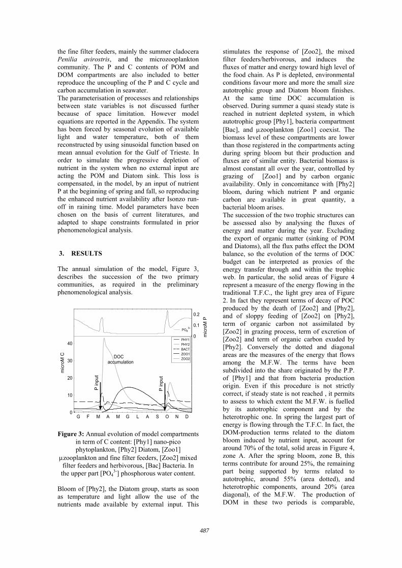
the fine filter feeders, mainly the summer cladocera Penilia avirostris, and the microzooplankton community. The P and C contents of POM and DOM compartments are also included to better reproduce the uncoupling of the P and C cycle and carbon accumulation in seawater. The parameterisation of processes and relationships between state variables is not discussed further because of space limitation. However model equations are reported in the Appendix. The system has been forced by seasonal evolution of available light and water temperature, both of them reconstructed by using sinusoidal function based on mean annual evolution for the Gulf of Trieste. In order to simulate the progressive depletion of nutrient in the system when no external input are acting the POM and Diatom sink. This loss is compensated, in the model, by an input of nutrient P at the beginning of spring and fall, so reproducing the enhanced nutrient availability after Isonzo run-off in raining time. Model parameters have been chosen on the basis of current literatures, and adapted to shape constraints formulated in prior phenomenological analysis. 3. RESULTS The annual simulation of the model, Figure 3, describes the succession of the two primary communities, as required in the preliminary phenomenological analysis.

mic

roM

C

mic

roM

P

0

0.1

0.2

0

10

20

30

40

G F M A M G L A S O N D

PHY1PHY2BACTZOO1ZOO2

P in

put

P in

put

DOCaccumulation

PO43-

Figure 3: Annual evolution of model compartments

in term of C content: [Phy1] nano-pico phytoplankton, [Phy2] Diatom, [Zoo1]

µzooplankton and fine filter feeders, [Zoo2] mixed filter feeders and herbivorous, [Bac] Bacteria. In the upper part [PO4

3-] phosphorous water content. Bloom of [Phy2], the Diatom group, starts as soon as temperature and light allow the use of the nutrients made available by external input. This

stimulates the response of [Zoo2], the mixed filter feeders/herbivorous, and induces the fluxes of matter and energy toward high level of the food chain. As P is depleted, environmental conditions favour more and more the small size autotrophic group and Diatom bloom finishes. At the same time DOC accumulation is observed. During summer a quasi steady state is reached in nutrient depleted system, in which autotrophic group [Phy1], bacteria compartment [Bac], and µzooplankton [Zoo1] coexist. The biomass level of these compartments are lower than those registered in the compartments acting during spring bloom but their production and fluxes are of similar entity. Bacterial biomass is almost constant all over the year, controlled by grazing of [Zoo1] and by carbon organic availability. Only in concomitance with [Phy2] bloom, during which nutrient P and organic carbon are available in great quantity, a bacterial bloom arises. The succession of the two trophic structures can be assessed also by analysing the fluxes of energy and matter during the year. Excluding the export of organic matter (sinking of POM and Diatoms), all the flux paths effect the DOM balance, so the evolution of the terms of DOC budget can be interpreted as proxies of the energy transfer through and within the trophic web. In particular, the solid areas of Figure 4 represent a measure of the energy flowing in the traditional T.F.C., the light grey area of Figure 2. In fact they represent terms of decay of POC produced by the death of [Zoo2] and [Phy2], and of sloppy feeding of [Zoo2] on [Phy2], term of organic carbon not assimilated by [Zoo2] in grazing process, term of excretion of [Zoo2] and term of organic carbon exuded by [Phy2]. Conversely the dotted and diagonal areas are the measures of the energy that flows among the M.F.W. The terms have been subdivided into the share originated by the P.P. of [Phy1] and that from bacteria production origin. Even if this procedure is not strictly correct, if steady state is not reached , it permits to assess to which extent the M.F.W. is fuelled by its autotrophic component and by the heterotrophic one. In spring the largest part of energy is flowing through the T.F.C. In fact, the DOM-production terms related to the diatom bloom induced by nutrient input, account for around 70% of the total, solid areas in Figure 4, zone A. After the spring bloom, zone B, this terms contribute for around 25%, the remaining part being supported by terms related to autotrophic, around 55% (area dotted), and heterotrophic components, around 20% (area diagonal), of the M.F.W. The production of DOM in these two periods is comparable,

487

despite the fact that sinking is reducing the amount of P available in the surface layer system. This implies that P is used more efficiently, namely recycled and re-used more rapidly in the second period. Indeed, the larger the part of energy which is flowing through the M.F.W., the shorter are the P cycle within the ecosystem, and the lesser the loss of matter via sinking of POM. Production of DOM is, of course, much smaller in winter time, zone C, in this period the largest part of energy is flowing again through the M.F.W., and specifically, through the heterotropic part of it, namely the Microbial Loop, Figure 4 zone C. During autumn, the P input stimulates new autotrophic production, but it is of short duration because water temperature and light no longer are at optimal condition for phytoplankton growth. In short, three different phases can be recognised: in spring time, the energy flows manly through the compartments of the TFC, after this the dominant trophic structure is the M.F.W. and in particular, the autotrophic component is the dominant path for energy during period B, while most of energy is flowing through the Microbial Loop in winter time.

mic

rom

ol C

/d

0

2

4

6

8

10

J F M A M J J A S O N D

Traditional Food ChainM.F.W. due to autotrophic

componentM.F.W. due to eterotrophic

component

BAC

+ µphy1

+ µphy1

- Toptphy1

- µphy1

- Kpphy2

+ µphy2

+ Toptphy1

- µphy1

+ µphy2

- Toptphy2

+Toptphy1

- kgrzoo1

- Toptphy1

+ Tmaxphy1

+ Swzoo1

- µbac+ µbac

- Kmbac

0.3

0.5

0.7

0.9 Total Phosphorus in the system

Figure 4: terms of DOC production: solid area represents the sum of fluxes from T.F.C., dotted

area represents the sum of terms of M.F.W. fuelled by P.P. of [Phy1], and diagonal area represents the

M.F.W. accounted to B.C.P. More important parameters controlling different terms of DOC

balance and state variables involved in different periods are superimposed.

4. SENSITIVITY ANALISYS Before to be used for investigation of processes going on in the Gulf, the model must be calibrated against real data collected in situ. On the other hand, only few among the parameters can be considered in the actual calibration procedure. In

order to select which are the most important parameters to focus on, we have performed a global Sensitivity Analysis, by implementing the Morris’s method [Saltelli et al., 2000]. Results of the analysis will be useful for improving our understanding of the functioning of the trophic food web of the Gulf. The Morris’s method allows to highlight the factors (model parameter) that have important or negligible effects on output model and to assess whether or not their effects are linear, and if the parameters have additive effects or interactions with other factors. Morris’s method is a screening method constructed on an individual randomised strict OAT (on-at-time) experiment design. The basic idea is to vary each parameter one-at-time and then compute the deviation of the model output from the last numerical experiment. The main effect of a factor is then estimated by computing a number of local measures (at different point, randomly extracted in the parameter space) and then taking the average of individual effects. This method reduces the dependence of the sensitivity analysis results on the choice of a specific starting point as happens in the local sensitivity methods. Therefore, it allows a global sensitivity analysis, even if individual interaction among parameters can not be quantified. The analysis returns, for each factor, a couple of numbers. The first one, µ, represents a measure of the importance of the factor, the second one, σ, is a measure of the non linearity of the factor, because of the presence of interaction with other factors. Model output, or indeed the more informative model response, has to be specified in advance. Our model describes the annual evolution of a trophic web system, forced by punctual input of nutrient and sinusoidal incident light and water temperature. In particular, we are interested in the capability of the model to shift, in dependence upon environmental conditions, between traditional food chain, and microbial food web as dominant energy flow paths. Therefore, it appears convenient to focus our analysis from one side on DOC mass balance (as before), and from the other one on sensitivities of state variables usually measured. Figure 5 illustrates, as an example of Morris results, influence of parameters on the ratio between energy flowing in the heterotrophic part of food web and the total energy flowing in the system, both computed on annual base, after a 5 years spin up. Maximum bacteria growth µbac and bacteria mortality Kmbac have the largest impact on such ratio, as indicated by their values on the horizontal axis (µ). The effects are, obviously, opposite, confirming the

488

relevance of bacteria density level in this process. Both parameters, however, act indirectly, or more precisely through non linear interactions with other factors. This is indicated by the values of σ (y axis). Other parameters are important as well, among these the temperature related parameters and the grazing ones.

µ

σ

0.0

0.2

0.4

0.6

0.8

1.0

1.2

1.4

−1.2 −0.8 −0.4 0.0 0.4 0.8 1.2

phy2

Topt_phy2

Topt_phy1

µ

Kmbackgrzoo1

Swzoo1

eff zoo1

ksink

bac

µ

Figure 5: sensitivity analysis results: example of Morris’s method (see text for explanation).

Analysis has been performed taking into consideration also sensitivity of state variables. Sensitivity of nutrient and plankton are particular relevant since they give an indication about how strongly the parameters can be constrained by assimilation of these variables. For each of the 2 periods individuated in the former analysis, indeed the spring and summer ones, the parameters which appear more suite for calibration are indicated in Figure 4. They are those parameters whose variation have the greatest effects on state variables and fluxes evolved in the different trophic structures. The sign indicates a negative or positive effect induced on the entity of fluxes by a positive variation of the parameter. 4. CONCLUSION The analysis of the ecosystem has allowed to formulate a model for the trophic food web that is the minimum complex structure able to describe the succession and dominance of the two trophic conditions and ecosystem energy paths. The model reproduces the succession of two primary communities, the first one, mainly represented by diatom species, start when external nutrient is supplied to the system, and the second, a well mixed of species of phytoplankton of small dimension, establishes during summer and is mainly based on recycling processes mediated by bacteria. Even if the maximum value of the biomass of the two autotrophic communities is quite different, as spring and summer trophic condition are different, the energy and matter fluxes they induce are comparable. The sensitivity analysis has highlighted the importance of only few parameters, mainly the constant of maximal growth rate for

bacteria and for phytoplankton groups temperature related parameters and grazing parameter. That is a useful result for the next step in the formulation of a more realistic model of the Gulf, namely calibration against experimental data. Further advances on the development of more comprehensive model of the ecosystem can be achieved by introducing transport processes description, modelling the cycle of other nutrients, as nitrogen and silicon, and introducing more realistic driving forces, based on experimental data and accounting for the environmental variability by the use of stochastic methodologies. 6. REFERENCES Cossarini G., Chemical, physical and biological

characteristics of the Gulf of Trieste: mini review. Technical report: 0023 OGA7, 2000.

Cushing D. H., A difference in structure between ecosystems in strongly stratified waters and in those that are only weekly stratified. Journal of Plankton Research, 11(1), 1-13, 1989.

Fonda Umani S., Pelagic production and biomass in the Adriatic Sea. Scientia Marina, 60(2), 65-77, 1996.

Legendre & F. Rassoulzadegan, Plankton and nutrient dynamics in marine water. Ophelia, 41, 153-172, 1995.

Malej A, P. Mozetic, V. Malacic, S. Terzic and M. Ahel. Phytoplankton responses to freshwater inputs in a small semi-enclosed gulf (Gulf of Trieste). Marine Ecology Progress Series, 120, 111-121. , 1995

Malej A., P.Mozetic, V. Malacic and V. Turk, Response of Summer Phytoplankton to Episodic Meteorological Events (Gulf of Trieste, Adriatic Sea). Marine Ecology, 18(3), 273-288 1997.

Mozetic P., S. Fonda Umani, B. Cataletto, and A. Malej, Seasonal and inter-annual plankton variability in the Gulf of Trieste (Northern Adriatic). ICES Journal of Marine Science, 55, 711-722,1998.

Saltelli A., K. Chan, E. M. Scott, Sensitivity Analysis. John Wiley & son, LTD., 2000.

Zavatarelli M., J.W. Baretta, J.G. Baretta-Bekker, N. Pinardi, The dynamics of the Adriatic Sea ecosystem. An idealized model study. Deep-Sea Research I, 47, 937-970, 2000

489

Appendix: Model Formulation

Model state variables: [PO4

3-] Phosphorus [µM P] [Bac] Bacteria [µM C] [Phy1] Phytopl. 1 (nano-picoplankton) [µM C] [Phy2] Phytopl. 2 (Diatoms) [µM C] [Quota] Phosphorus quota in Diatom [µM P:µM C]I I light incident [lux] [Zoo1] Zoopl. 1 (µzooplankton) [µM C] [Zoo2] Zoopl. 2 (M.F.F. & Herb.) [µM C] [DOP] Dissolved Organic Phosphorus [µM P] [DOC] Dissolved Organic Carbon [µM C] [DetP] Detritus phosphorus [µM P] [DetC] Detritus carbon [µM C] Model formulation:

1_111134 ]1[]1[]1[])([)()(]1[

phyzoorrtphyphyphy GrazPhyAKrPhyKmPhyPOfIfTfdtPhyd

−⋅⋅−⋅−⋅⋅⋅⋅= − µ

]2[]2[]2[]2[])([])([)()(]2[2_2222

34 PhywGrazPhyAKrPhyKmPhyQuotafPOfIfTf

dtPhyd

sdphyzoorrtphyphyphy ⋅−−⋅⋅−⋅−⋅⋅⋅⋅⋅= − µ

][])([])([)()(][])([][2

34

minmax

max344 QuotaQuotafPOfIfTf

QQQuotaQPOfV

dtQuotad

phypo ⋅⋅⋅⋅⋅−−

−⋅⋅= −− µ

baczoorrtBacBac GrazBacAKmBacPOfDOCfTfdtBacd

_134 ][][])([)()(][

−⋅⋅−⋅⋅⋅⋅= − µ

( ) ]1[)(]1[]1[11_11_11 ZooTfKexcrZooKmGrazGrazeff

dtZood

zoozoobaczoophyzoozoo ⋅⋅−⋅−+⋅=

]2[)(]2[]2[222_222 ZooTfKexcrZooKmGrazeffRg

dtZood

zoozoophyzoozoozoo ⋅⋅−⋅−⋅⋅=

][][])([)()(

]2[][

])([]1[])([)()(][

_34_

minmax

max3441

341_

34

BacAKmrFBacPOfDOCfTfr

PhyQQ

QuotaQPOfVPhyPOfIfTfr

dtPOd

rrtbacbacpcPhosphateBacbacpc

pophyphypc

⋅⋅⋅++⋅⋅⋅⋅⋅−

⋅−

−⋅⋅−⋅⋅⋅⋅⋅−=

−

−−−

µ

µ

2_2234

2121det

][])([)()(

]2[)(]1[)(]2[)(]1[)(][][

phyzoozooDOCBac

phyphyzoozoorrtC

GrazeffRgBacPOfDOCfTf

PhyTfKrPhyTfKrZooTfKexcrZooTfKexcrDetCAKdecdt

DOCd

⋅⋅+⋅⋅⋅⋅−

⋅⋅+⋅⋅+⋅⋅+⋅⋅+⋅⋅=

− µ

( ){ } [ ] PhosphatephyphypcphyphyzoozooDOPzoozoopc

zoozoopcbaczoobacbacpcbaczoozoozoopcbacpcrrtP

FPhyTfKrrQuotaPhyTfKrGrazeffRgZooTfKexcrr

ZooTfKexcrrGrazeffrGrazeffrrDetPAKdecdt

DOPd

−⋅⋅⋅+⋅⋅⋅+⋅⋅+⋅⋅⋅

+⋅⋅⋅+⋅⋅+⋅⋅−+⋅⋅=

]1[)(]2[)(]2[)(

]1[)(][][

11_22_2222_

11__1__111__det

( ) ( )

sinkCDetCAKdec

ZooKmZooKmPhyKmPhyKmGrazeffGrazeffdt

DetCd

rrtC

zoozoophyphyphyzoozoophyzoozoo

−⋅⋅−

⋅+⋅+⋅+⋅+⋅−+⋅−=

][

]2[]1[]2[]1[11][

det

21212_221_11

( ){ } ( ){ } [ ]sinkPDetPAKdecZooKmr

ZooKmrQuotaPhyKmGrazeffrPhyKmGrazeffdt

DetPd

rrtPzoozoopc

zoozoopcphyphyzoozoophypcphyphyzoozoo

−⋅⋅−⋅⋅+

⋅⋅+⋅⋅+⋅−+⋅⋅+⋅−=

][]2[

]1[]2[1]1[1][

det22_

11_22_221_11_11

Model Parameter: µphy_i [t-1] max growth rate for i=Phy1, Phy2 Vpo4 [µMP/µMC/t] max P uptake rate for Phy2 µbac [t-1] max growth rate for Bac Tmax_i [T] Temperature maximal for i=Phy1, Phy2, Bac Topt_i [T] Temperature optimal for i=Phy1,Phy2,Bac Qmin [µMP:µMC] minimal P quota for Phy2 Qmax [µMP:µMC] maximal P quota for Phy2 kcl [µMP:µMC] critical quota level for Phy2 Kp_i [µM P] halfsaturation constant for i=Phy1, Phy2, Bac KDOC [µM C] Semisaturation constant for Bac Iopt_i [lux] optimal light intensity for i= Phy1,Phy2 Kep_i [T-1] exponential factor Km _i [t-1] max mortality rate for i=Phy1, Phy2, Bac Kr i [t-1] max respiration rate for i=Phy1, Phy2, Bac Kexczoo_i [t-1] max excretion rate for i=Zoo1, Zoo2 Km zoo_i [t-1] max mortality rate for i=Zoo1, Zoo2 Kgrzoo_i [t-1] max grazing rate for i=Zoo1, Zoo2 Swzoo1 prey preference parameter for Zoo1 Kfzoo1_ [µM C2] halfsaturation constant of grazing for Zoo1 Kfzoo2_ [µM C] halfsaturation constant of grazing for Zoo2 effzoo_i efficiency ingestion for i=Zoo1, Zoo2 Kdec_i [t-1] decay rate for i=DetC, DetP Ksink [t-1] sinking rate for Detritus compartments rpc_phy1 [µMP/µMC] Carbon Phosphorus ration in Phy1 rpc_bac [µMP/µMC] Carbon Phosphorus ration in Bac rpc_zoo_i [µMP/µMC] Carbon Phosphorus ration for i= Zoo1, Zoo2 Vphosp [µMP/µMC/t] max phosphatase rate KDOP [µM P] Semisaturation constant for phosphatase Wsd Sinking rate for Diatom

[ ][ ] [ ]2

22

222_2 zoo

KfPhyPhyKgrGraz

zoozoophyzoo ⋅

+⋅=

[ ][ ] [ ]

[ ]11

2

12

122

2

11_1 zooKfSwBacPhy

PhyKgrGrazzoozoo

zoophyzoo ⋅+⋅+

⋅=

[ ][ ] [ ]

[ ]11 1

21

22

21

2

1_1 zooKfSwBacPhy

SwBacKgrGraz

zoozoo

zoozoobaczoo ⋅

+⋅+

⋅⋅=

[ ][ ] [ ]Bac

kDOPDOPVF

DOPphosPhosphate ⋅

+⋅=

[ ] sinkii KDetsink ⋅= [ ][ ] [ ]Bac

KDOPDOPVPhosph

DOPsphos ⋅

+⋅=

( ) ( )( )

( )( )iopt

iopti

TTiKepTTiKep

iopti

i eTT

TTTf _

_max_

__

_max_

max_ −⋅

−⋅

⋅

−

−=

( ) iPhyIoptI

iPhy

eIopt

IIf ⋅= [ ]( ) [ ]

[ ]iPhyKpPO

POPOf+

= −

−−

34

343

4

[ ]( ) [ ][ ] clkQuota

QQuotaQuotaf+

−= min

[ ]( ) [ ]

[ ] DOCKDOCDOCDOCf

+=

[ ] [ ]

[ ]

−===

<

2_

2_

1

0

2

2_

zoopc

zoopc

rQuota

zoo

rQuota

DOC

DOP

zoopc

RgRgRg

rquotaif

[ ][ ]

==

−=≥

1 0

2

2_

2_

zoo

DOC

zoopcDOP

zoopc

RgRg

rQuotaRgrquotaif

( )TArrt −= 2010

490