Article

A Model-Driven Co-Design Framework for FusingControl and Scheduling Viewpoints

Sakthivel Manikandan Sundharam 1,* ID , Nicolas Navet 1, Sebastian Altmeyer 2 ID Lionel Havet 3

1 Laboratory of Advanced Software Systems (LASSY), CSC Research Unit, University of Luxembourg, Maisondu Nombre, L-4364 Esch-sur-Alzette, Luxembourg; nicolas.navet@uni.lu

2 CSA Group, University of Amsterdam, 1098XH Amsterdam, Netherlands; altmeyer@uva.nl3 RealTime-at-Work (RTaW), 4 Rue Piroux, 54000 Nancy, France; lionel.havet@realtimeatwork.com* Correspondence: sakthivel.sundharam@uni.lu; Tel.: +352-466-644-5132

Received: 12 December 2017; Accepted: 14 February 2018; Published: 20 February 2018

Abstract: Model-Driven Engineering (MDE) is widely applied in the industry to develop newsoftware functions and integrate them into the existing run-time environment of a Cyber-PhysicalSystem (CPS). The design of a software component involves designers from various viewpoints suchas control theory, software engineering, safety, etc. In practice, while a designer from one disciplinefocuses on the core aspects of his field (for instance, a control engineer concentrates on designinga stable controller), he neglects or considers less importantly the other engineering aspects (forinstance, real-time software engineering or energy efficiency). This may cause some of the functionaland non-functional requirements not to be met satisfactorily. In this work, we present a co-designframework based on timing tolerance contract to address such design gaps between control andreal-time software engineering. The framework consists of three steps: controller design, verified byjitter margin analysis along with co-simulation, software design verified by a novel schedulabilityanalysis, and the run-time verification by monitoring the execution of the models on target. Thisframework builds on CPAL (Cyber-Physical Action Language), an MDE design environment basedon model-interpretation, which enforces a timing-realistic behavior in simulation through timingand scheduling annotations. The application of our framework is exemplified in the design of anautomotive cruise control system.

Keywords: model-driven engineering; control software; timing tolerance contract; controller model;schedulability; stability; input jitters; varying execution-times; output jitters; input-to-output delay;co-simulation; real-time scheduling; control system performance

1. Introduction

Control theory and software engineering are two disciplines involved in the development ofcontrol software. Traditionally, control engineers design the controller model without consideringthe computing platform constraints and specifications. The converse applies to software engineering,where control performance is not considered during software design. The control engineering andthe software engineering are two different worlds with different objectives in mind. Consequently,the complete set of functional and non-functional requirements of the control software are usuallynot elicited at the control design stage. Hence, as discussed in [1], substantial design-gaps may existduring the design of a control software.

The control software executes on an Electronic Control Units (ECU) interfaced with varioussensors and actuators. The continuous-time signals are periodically sampled; each sampled set of datais then processed by real-time control functions. Control theory typically assumes deterministic andperiodic sampling. However in practice, for instance, due to preemptions and varying task execution

Sensors 2018, 18, 628; doi:10.3390/s18020628 www.mdpi.com/journal/sensors

Sensors 2018, 18, 628 2 of 26

times, there exists a varying delay between sensing and actuation, which is called input-to-outputdelay or sensing-to-actuation delay. A control designer typically assumes this input-to-output delayto be zero or constant which is an unrealistic assumption. The input-to-output delay depends on thetime at which sensing and actuation takes place. Sensing time may also vary over time typically dueto the interference of higher priority tasks, and the variability of sensing times is called input jitter.There are also jitters in the actuation times, called output jitters caused by varying execution times andpreemptions. These jitters directly impact the quality of control functions, and, in the worst-case, theymight jeopardize the safety of the system. Hence, it is important to consider these delays during thedesign phase of the control software. This work addresses the case where the input data acquisition isdone locally on one node. It can be extended like in TrueTime [2] to cover the case of networked controlsystems, including "Industrial Internet of Things" (IIoT) applications, where data are transmitted overa network, which would increase the input jitters, as well as the input-to-output delays.

1.1. State-of-the-Art

A survey of tools and methods developed to address this problem is presented in [3]. Most ofthe techniques discussed in this survey are based on co-design approaches. Directly relevant to ourwork are TrueTime [2] and T-Res [4] which are simulation tools that can consider how the timingbehavior of the implementation affects the performance of the control. Both approaches use Simulinkfor control design and timing extension toolboxes to include computing aspects, foremost the effectsof task scheduling on the control performance. In a recent study [5], we discussed our co-design andsimulation environment and compared it with these state-of-the-art tools. Our co-design techniquemainly differs from these approaches by allowing the control model to be directly executed (by aninterpreter engine) on the target hardware, without changing a single line of code. The benefits arereduced development time and avoidance of distortions (i.e., semantic gaps) between the simulatedand executed control programs. On the other hand, TrueTime and T-Res are essentially simulationenvironments that involve a step of model-to-code transformation (typically code generation), whichmay risk widening the semantic gap between model and executable code, requiring additionaldevelopment effort. Generally speaking, the existing co-design simulation techniques are mainlyconcerned with enabling the study of the effect of timing variabilities on control performance, ratherthan addressing the design gaps between control and software viewpoints. Other works [1,6] presentco-engineering techniques where the initial controller is integrated in a virtual ECU. The behaviorof the controller is then assessed through timing analysis tools whose results are injected into thecontroller model. This approach shares similarities with ours but it relies on expensive and proprietarytiming analysis tools and remains at the model level (i.e., implementation is abstracted).

1.2. Contributions

In this paper, we propose a framework that supports our co-design modeling environment forboth controller and control software development. The framework provides schedulability and controlperformance analysis along with simulation capabilities. We underpin the proposed framework withthe help of timing contracts introduced in [7] which are sets of timing characteristics that ensure thetargeted control performance. The timing contract can be a crucial concept in component-based designbecause it drives and synergizes the design thinking of the stakeholders from different viewpoints.We use the timing contract as a candidate to bridge the control software design-gaps. During theapplication of a timing contract, we observe a vertical type contract [8] in our proposed framework asthe timing contract is applied between two phases of the Software Development Life Cycle (SDLC), inthis case between controller design and software development.

The co-design framework presented in this work encompasses three steps of the developmentcycle: (i) controller design, (ii) software scheduling and execution platform configuration, and (iii)run-time monitoring. Firstly, we discuss scheduling and stability viewpoint analyses supportingthe proposed co-design and simulation environment. We rely on our timing-aware model-driven

Sensors 2018, 18, 628 3 of 26

environment called Cyber-Physical Action Language (CPAL) for co-design in Simulink. We thenpresent the CPAL constructs and timing annotations, central to our approach, which enable us toreproduce the timing irregularities of interest, such as jitters and varying input-to-output delays.CPAL provides the timing dimension to the controller design, which acts on the plant model inSimulink. We provide the CPAL execution platform for Simulink as open access for experimentation.Along with existing jitter analysis tools, the proposed co-design platform helps designing stabilityguaranteed controller models by integrating the target-platform timing behavior. Furthermore, itprovides software engineering with the control information needed to bound the space of feasiblesoftware design solutions. The stability verification itself is done with the help of the jitter marginconcept and the co-simulation of CPAL execution in the Simulink environment.

The second contribution is the verification of the timing tolerance contract assumptions madeduring controller design. The verification is specifically useful when a new control function isintegrated into an existing stable and functioning ECU. How can we analytically validate whether thesystem maintains the desired performance (stable and schedulable) after integration? To this end, wepropose a novel schedulability analysis for a certain class of task and execution models in real-timescheduling. To assign a realistic execution time to the controller task, we estimate the Worst-CaseExecution Time (WCET) beforehand using measurements of the model running on the target hardware.

The third and last contribution is the proposed run-time verification methodology. During modelon target execution, we check whether the newly integrated controller function stays within thestability margin. For this, we take advantage of CPAL introspection features to monitor the executioncharacteristics of a controller model at run-time. More specifically, we introspect whether the jitters andinput output latencies are within the margin guaranteeing the stability and schedulability objectives.

1.3. Structure

This paper is structured as follows. In Section 2, we explain the system model and the stepsinvolved in the framework for fusing control and scheduling viewpoints. Section 3 presents theproposed co-modeling and simulation environment as well as jitter analysis tools and methods. InSection 4, we explain the verification of timing tolerance assumptions using WCET measurements andthe schedulability analysis. In Section 5, we evaluate the framework using the example of a cruisecontrol system. In the same section, we discuss the stability verification using the jitter margin conceptand the CPAL co-simulation in Simulink. The section also details the scheduling configuration andrun-time introspection features. Section 6 provides the related work. Section 7 concludes the paper.

2. Framework for Fusing Control and Scheduling Viewpoints

System designers in the industry are typically highly knowledgeable in their own fields (controlsystems, software engineering, scheduling, etc.) but contracts among design teams are not necessarilywell established and communicated among the stakeholders. Our objective is to define a structuredframework, with clear interfaces, which can be agreed upon and followed by all. The frameworkproposed in this section highlights the issues faced at each step of the design and we propose possiblesolutions. Our framework may not be suitable for all industrial settings, but it addresses the gapbetween control models and their implementation, and can serve as a basis for context-specific designframeworks.

2.1. System Model

We propose an integrated framework which combines the tools and methods necessary to designa model of the system. Table 1 provides a quick reference for the notations used in this paper. Thesystem is comprised of a controller model, a plant model and platform model. Plant P is modeled by acontinuous-time system of equations

Sensors 2018, 18, 628 4 of 26

x = Ax + Bu,

y = Kx,(1)

where x is the plant state and u is the control signal. The plant output y is sampled periodically withsome delays at discrete time instants. The control signal is updated periodically with some delays atdiscrete time instants, (i.e., actuation also happens with some delay). Quantities A, B, K are constants.The controller model is comprised of a task set Γ of n periodic tasks {T1, . . . Tn} executing on a singleprocessor.

Table 1. Notations used in the paper.

task-set Γ = {T1, . . . Tn}pseudo task-set Γ = {T1, . . . Tn}number of tasks n ε N

job index i, j ε Ntask worst-case execution time with no interference Ci ε R

task period hi ε Rtask relative deadline Di ε R

task absolute deadline di ε Rtask release time ri ε R

task finish time fi ε Rtask worst-case response time Rw

i ε Rtask best-case response time Rb

i ε Rtask processor demand PDi ε R

task busy-period L ε Rinput jitter also known as sampling jitter Jh ε R

output jitter also known as response-time jitter Jτ ε Rinput-to-output delay also known as StA latency τ ε R

k-th sensing time instance tsk ε R

k-th actuation time instance tak ε R

nominal input-output delay L ε R

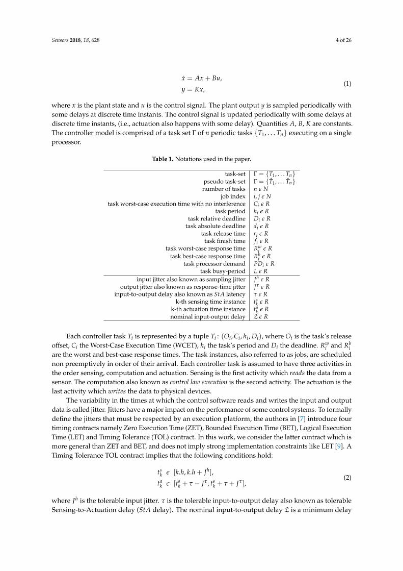
Each controller task Ti is represented by a tuple Ti : (Oi, Ci, hi, Di), where Oi is the task’s releaseoffset, Ci the Worst-Case Execution Time (WCET), hi the task’s period and Di the deadline. Rw

i and Rbi

are the worst and best-case response times. The task instances, also referred to as jobs, are schedulednon preemptively in order of their arrival. Each controller task is assumed to have three activities inthe order sensing, computation and actuation. Sensing is the first activity which reads the data from asensor. The computation also known as control law execution is the second activity. The actuation is thelast activity which writes the data to physical devices.

The variability in the times at which the control software reads and writes the input and outputdata is called jitter. Jitters have a major impact on the performance of some control systems. To formallydefine the jitters that must be respected by an execution platform, the authors in [7] introduce fourtiming contracts namely Zero Execution Time (ZET), Bounded Execution Time (BET), Logical ExecutionTime (LET) and Timing Tolerance (TOL) contract. In this work, we consider the latter contract which ismore general than ZET and BET, and does not imply strong implementation constraints like LET [9]. ATiming Tolerance TOL contract implies that the following conditions hold:

tsk ε [k.h, k.h + Jh],

tak ε [ts

k + τ − Jτ , tsk + τ + Jτ ],

(2)

where Jh is the tolerable input jitter. τ is the tolerable input-to-output delay also known as tolerableSensing-to-Actuation delay (StA delay). The nominal input-to-output delay L is a minimum delay

Sensors 2018, 18, 628 5 of 26

experienced between input to output. Jτ is the tolerable output jitter. The tolerances Jh and Jτ are alsoreferred to as margins, namely input jitter margin and output jitter margin.

2.2. Framework Steps

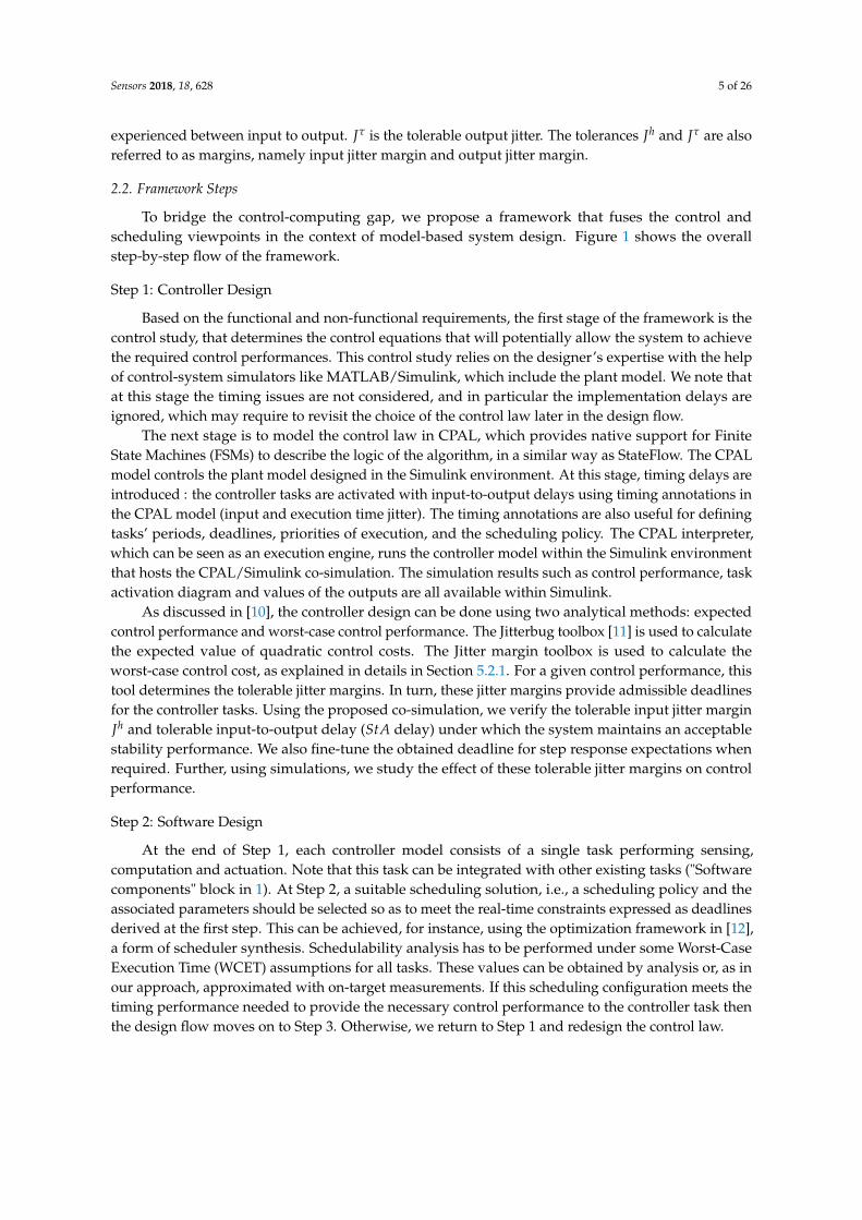
To bridge the control-computing gap, we propose a framework that fuses the control andscheduling viewpoints in the context of model-based system design. Figure 1 shows the overallstep-by-step flow of the framework.

Step 1: Controller Design

Based on the functional and non-functional requirements, the first stage of the framework is thecontrol study, that determines the control equations that will potentially allow the system to achievethe required control performances. This control study relies on the designer’s expertise with the helpof control-system simulators like MATLAB/Simulink, which include the plant model. We note thatat this stage the timing issues are not considered, and in particular the implementation delays areignored, which may require to revisit the choice of the control law later in the design flow.

The next stage is to model the control law in CPAL, which provides native support for FiniteState Machines (FSMs) to describe the logic of the algorithm, in a similar way as StateFlow. The CPALmodel controls the plant model designed in the Simulink environment. At this stage, timing delays areintroduced : the controller tasks are activated with input-to-output delays using timing annotations inthe CPAL model (input and execution time jitter). The timing annotations are also useful for definingtasks’ periods, deadlines, priorities of execution, and the scheduling policy. The CPAL interpreter,which can be seen as an execution engine, runs the controller model within the Simulink environmentthat hosts the CPAL/Simulink co-simulation. The simulation results such as control performance, taskactivation diagram and values of the outputs are all available within Simulink.

As discussed in [10], the controller design can be done using two analytical methods: expectedcontrol performance and worst-case control performance. The Jitterbug toolbox [11] is used to calculatethe expected value of quadratic control costs. The Jitter margin toolbox is used to calculate theworst-case control cost, as explained in details in Section 5.2.1. For a given control performance, thistool determines the tolerable jitter margins. In turn, these jitter margins provide admissible deadlinesfor the controller tasks. Using the proposed co-simulation, we verify the tolerable input jitter marginJh and tolerable input-to-output delay (StA delay) under which the system maintains an acceptablestability performance. We also fine-tune the obtained deadline for step response expectations whenrequired. Further, using simulations, we study the effect of these tolerable jitter margins on controlperformance.

Step 2: Software Design

At the end of Step 1, each controller model consists of a single task performing sensing,computation and actuation. Note that this task can be integrated with other existing tasks ("Softwarecomponents" block in 1). At Step 2, a suitable scheduling solution, i.e., a scheduling policy and theassociated parameters should be selected so as to meet the real-time constraints expressed as deadlinesderived at the first step. This can be achieved, for instance, using the optimization framework in [12],a form of scheduler synthesis. Schedulability analysis has to be performed under some Worst-CaseExecution Time (WCET) assumptions for all tasks. These values can be obtained by analysis or, as inour approach, approximated with on-target measurements. If this scheduling configuration meets thetiming performance needed to provide the necessary control performance to the controller task thenthe design flow moves on to Step 3. Otherwise, we return to Step 1 and redesign the control law.

Sensors 2018, 18, 628 6 of 26

Mo

del

on

Tar

get

(Ste

p 3

)C

on

tro

ller

des

ign

(St

ep

1)

Soft

war

e d

esig

n (

Ste

p 2

)M

od

el in

tro

spe

ctio

n (

Ste

p 3

)C

on

tro

ller

des

ign

(St

ep

1)

Soft

war

e d

esig

n (

Ste

p 2

)

Calculate Jh and Jτ

Jitter margin tools

Check period, WCET, jitters at run-time

Functional and non functional

requirements

Modeling CPAL controller

No

Measuring WCET CPAL code on target

WCET

Yes

Functional controller with feasible

scheduling parameters

Model on Target that guarantee stability and

schedulability

Performance assumption met?

No

Yes

Synthesize scheduler

Is schedulable?schedulability analysis

Co-simulation CPAL in Simulink

Check period, WCET, jitters at run-time

Functional and non functional

requirements

Control study

admissible deadline

Measuring WCET CPAL code on target

WCET

Functional controller with feasible

scheduling parameters

No

Model on Target that guarantee stability and

schedulability

Performance assumption met ?

No

Yes

Synthesize scheduler

Is schedulability analysis passed ?

Yes

Optimizing the CPAL code

123

Re

-de

sign

co

ntr

olle

r

Mo

dif

y ji

tte

r m

arg

ins

Analytical methodsTiming accurate simulation

Software components

Tim

ing

tole

ran

ce a

ssu

mp

tio

ns

veri

fica

tio

nT

arge

t ru

n-t

ime

ver

ific

ati

on

St

ab

ilit

y g

ua

ran

tee

d c

on

tro

ller

Figure 1. Illustration of framework flow for fusing control and scheduling viewpoints. The dashedpart in the software design step is out-of-scope of this paper.

Sensors 2018, 18, 628 7 of 26

The same CPAL model executed in the simulation environment (in the previous step) is nowinterpreted directly on the target to measure the execution time of the task. Schedulability analysiscan then be performed, and we propose a novel schedulability analysis for FIFO policy with offsets inSection 4. Although FIFO is outperformed by most policies in terms of meeting deadlines [13], it hasthe advantage that the scheduling order does not depend on the execution times, irrespective of theplatform. The schedulability analysis checks whether the controller task we integrate with the existingsoftware components remains schedulable or not.

This stage, if successful, ensures that the timing constraints coming from the control laws are metby the software and execution platform. If unsuccessful, we can first try to optimize the CPAL code.This may include breaking down the controller task into sub-tasks, for instance one for sensing, onefor computation and one for actuation, which is a classical strategy to increase the schedulability ofcontrol systems [14], but in some cases the suitable strategy has to be specific to the application. If stillunsuccessful, the process returns to Step 1 for a redesign or fine-tuning of the controller. In any cases,the model used at Step 1 for functional simulation will be the one used for execution on the targethardware.

Step 3: Model Introspection

From Step 2, we obtain a functional CPAL controller along with the scheduling parameters to beconfigured for on-target execution. These parameters have been derived from the models. To makesure that there is no distortion between the model’s assumptions and the execution, task characteristicssuch as period, offset, jitter, priority, deadline as well as the activation time of the current and previousinstances are monitored during execution using the CPAL introspection features. In Section 5, wediscuss the monitoring of CPAL model execution at run-time, especially the monitoring of timingtolerance specifications such as input jitters, output jitters and the input-to-output delays.

3. Analysis and Co-Simulation of Controller Design

This section explains the controller design using analytical methods and co-simulation. The resultof this stage is a controller whose stability and more generally performance are guaranteed undercertain assumptions on the worst-case timing behavior of the software implementation.

3.1. Jitter Analysis

Jitter analysis is performed using two evaluations, namely the evaluation of the expected controlperformance, and of the worst-case control performance. For instance, the Jitterbug toolbox [11] can beused to calculate the expected value of quadratic control costs. This measure in the general case is notsufficient to guarantee the stability of the plant [10], but stability can be verified through worst-casecontrol performance analysis. In our framework, the technique presented in [15] and implemented inthe jitter margin toolbox is used for the derivation of the jitter margins, both input and input-to-outputdelays, ensuring stability under the worst-case control performance. The calculated jitter marginsimply the maximum deadline for a controller task. This theoretical bound on the deadline derived byanalysis may be further fine-tuned by simulation as explained in the next subsections.

3.2. Controller Modeling in CPAL

CPAL, short for Cyber-Physical Action Language, is a modeling and discrete-event simulationlanguage for cyber-physical systems [16]. CPAL serves as a design-exploration platform with graphicalrepresentation. The models can be executed both in simulation mode as well as in real-time modeon an embedded target. CPAL is a lightweight execution engine (around 10, 000 lines of C code)designed for timing predictability that can run on top of an OS or without any OS, and thus withoutthe interferences the OS would create.

In case of simulation, execution is as fast as possible according to a logical clock and not thephysical time (see [17]). Typically, executing in simulation mode is several orders of magnitude faster

Sensors 2018, 18, 628 8 of 26

than in real-time mode. The controller code executes in zero-time during simulation, except if it usespredefined CPAL timing annotations. The simulation mode CPAL interpreter is an execution enginehosted by an operating system. The simulation execution can be carried out in a stand-alone built-insimulation environment [18] or it can be used in co-simulation environments, for instance as in thiswork integrated in MATLAB/Simulink as an S-function. CPAL aims to achieve the same temporalbehavior in simulation mode and real-time mode on the target. This property is referred to as timingequivalence. It can be achieved through timing annotations to inject delays in the simulation model.Figure 2 illustrates the CPAL timing annotations to inject input and output jitters in a control model.

Figure 2. Simulating random input and output jitters affecting a CPAL controller model using timingannotations. Level 1 means that the controller is being executed.

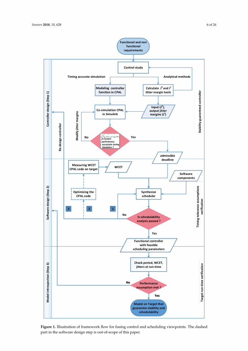
Like other modeling environments for control programs such as StateFlow, CPAL providessupport for Finite State Machines (FSMs) with conditional and timed transitions. As can be seenin Figure 3, transitions can happen either when a boolean condition is true, after a certain timeduration is spent in the active state, or the conjunction of both. A distinctive feature of CPAL is thatit relies on model interpretation: a CPAL model verified by simulation can be executed directly onan embedded target such as ARM Cortex - M4 (FRDM K64F) and ARM Cortex - A7 (RaspberryPi). Model-interpretation is well suited for rapid-prototyping [19] and prevents any distortionbetween models and code that could be introduced during code generation. A disadvantage ofmodel interpretation is that it is slower than compiled code. For that reason, it is not always a practicalsolution for on-target execution. For the purpose of simulation on desktop machines, the executiontime of the control part is however not an issue, especially in a co-simulation environment wheresimulating the plant is by far the most time-consuming task.

The CPAL documentation, a graphical editor and the execution engine for various desktop andembedded platforms are freely available at http://www.designcps.com. The CPAL control libraryas in Figure 4 needed to execute in MLSL controller models written in CPAL, and the models toreproduce the experiments of this paper are freely available at https://www.designcps.com/wp-content/uploads/cpal_codesign_framework.zip.

3.3. Co-simulation in MATLAB/Simulink

In our proposed co-simulation approach, a controller model is designed in CPAL, and theplant model in Simulink. Controllers can easily be designed in Simulink too. However, Simulinkout-of-the-box is not offering possibilities to study the performance of control loops subject toscheduling and networking delays. Indeed, varying execution times, preemption delays, blockingdelays, kernel overheads cannot be captured in the standard Simulink environment. This can be doneonly with TrueTime [2], which, to the best of our knowledge, is the most widely used tool in thereal-time and control communities to study control performance subject to timing irregularities. Oneshould also cite T-Res [4], a more recent and modular version of TrueTime.

Sensors 2018, 18, 628 9 of 26

Figure 3. CPAL program illustrating the native support for FSM, conditional and timed state transitions.The top-left graphic is the representation of the FSM embedded in a process, while the bottom-leftgraphic is the functional architecture with the flows of data, as both seen in the CPAL-editor.

Pendulum Angle Force

Cart Position

Simscape

Scope20

1

100

0 reference

100

ForceImpulse

kp_in

ki_inp_out kd_in

controller.astfilterGain_in

angle_in

reference_in

force_out

i_out

d_out

CPAL CONTROLLER

Add4

Controller model in CPAL Plant model in Simulink

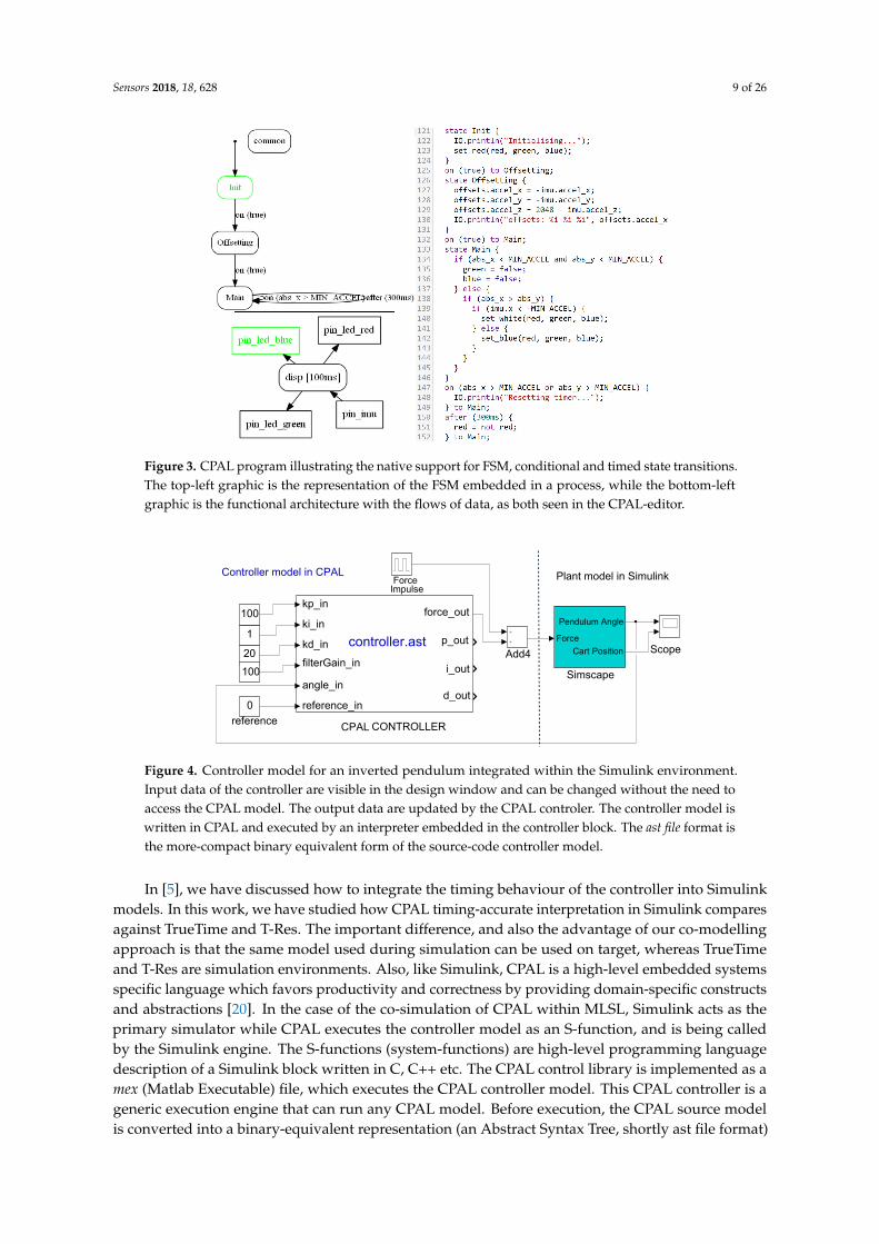
Figure 4. Controller model for an inverted pendulum integrated within the Simulink environment.Input data of the controller are visible in the design window and can be changed without the need toaccess the CPAL model. The output data are updated by the CPAL controler. The controller model iswritten in CPAL and executed by an interpreter embedded in the controller block. The ast file format isthe more-compact binary equivalent form of the source-code controller model.

In [5], we have discussed how to integrate the timing behaviour of the controller into Simulinkmodels. In this work, we have studied how CPAL timing-accurate interpretation in Simulink comparesagainst TrueTime and T-Res. The important difference, and also the advantage of our co-modellingapproach is that the same model used during simulation can be used on target, whereas TrueTimeand T-Res are simulation environments. Also, like Simulink, CPAL is a high-level embedded systemsspecific language which favors productivity and correctness by providing domain-specific constructsand abstractions [20]. In the case of the co-simulation of CPAL within MLSL, Simulink acts as theprimary simulator while CPAL executes the controller model as an S-function, and is being calledby the Simulink engine. The S-functions (system-functions) are high-level programming languagedescription of a Simulink block written in C, C++ etc. The CPAL control library is implemented as amex (Matlab Executable) file, which executes the CPAL controller model. This CPAL controller is ageneric execution engine that can run any CPAL model. Before execution, the CPAL source modelis converted into a binary-equivalent representation (an Abstract Syntax Tree, shortly ast file format)

Sensors 2018, 18, 628 10 of 26

using the CPAL parser. The Simulink engine interacts with the CPAL model through data flows andcontrol flows. Data flow, for instance force_ out in Figure 4, are used for the exchange of informationbetween the Simulink engine and the CPAL controller, while the control flows define when Simulinkinvokes the CPAL S-function.

The implementation is discrete-event-based simulation using Simulink built-in zero-crossingdetection. The concept of tasks and real-time schedulers are available natively in CPAL. The defaultCPAL scheduling policy is FIFO, but CPAL also supports Non-Preemptive Earliest Deadline First(NP-EDF) and Fixed Priority Non-Preemptive (FPNP). In Figure 5, we show the instantiation of acontroller task and the task parameters with the delays and jitters. A timing annotation can also specifythe scheduling policy if the controller consists of several tasks. Simulation of the plant dynamicsis carried-out by computing model states at successive time steps over a specified duration. Thiscomputation is done by a solver provided in Simulink. Since our overall model is discrete, a variablestep size solver is used in our co-simulation approach. The rationale behind this choice is that for thetiming analysis of real-time control systems, it is necessary to reduce the step size (when needed) toincrease the accuracy when model states are changing rapidly during zero crossing events. Section 5.1presents an example co-simulation of a simplified cruise control system.

Figure 5. Snippet of CPAL code instantiating a controller of period 10 ms and offset 2 ms and specifyingthe variation of the input jitter Jh and the input-to-output delay τ during a simulation run. This isachieved through a timing annotation executed in simulation, but ignored once on target.

4. Timing Verification Using Schedulability Analysis

The next step in the framework is the timing verification of the controller model designed in theprevious step. From the jitter margins, we derive the deadlines of the controller task(s). Typically, itwill be a single task, but the controller can also be implemented as several tasks such as an input task,a computation task and an output task. The deadlines will be used for the scheduler synthesis andschedulability analysis. To obtain realistic Worst-Case Execution Times (WCET) for the schedulabilityanalysis, we use a measurement-based technique in which the controller model is executed on thetarget hardware.

4.1. Worst-Case Execution Time (WCET) Measurement

The CPAL controller model which we executed earlier in the co-simulation environmentis now uploaded to the target platform to estimate the WCET by measurements. The CPALmodel-interpretation engine is specific to a target platform, it can be executed on top of an OperatingSystem (OS) or without an OS, the latter being called Bare-Metal Model Interpretation (BMMI). Thereare two ways to estimate the WCETs: using a logic analyzer or taking advantage of CPAL in-builtexecution-time measurement feature. The latter possibility is only available when CPAL is hostedby an OS, as freeRTOS, embedded Linux or Raspbian. It does not require connecting the target toan external measurement device and instrumenting the code, and thus provides a quick method toestimate the WCET. It is, however, less accurate than measurements using logic analyzer, since itinvolves additional run-time overhead in the interpretation engine.

Sensors 2018, 18, 628 11 of 26

For the discrete-time PID controller used in Section 5, the measured WCET of the CPAL controllertask using logic analyzer is 34.4 µs on a Raspberry Pi2 model B. This can also be obtained using thein-built feature of CPAL –-stats, a command-line option to be used when we execute the model ontarget. When we remove the code of the actual control algorithm, leaving just the skeleton of thetasks, we can observe the scheduler overhead, which amounts to 155 µs. When we execute the modelas it is, we observe the scheduler overhead plus the execution time of the task to be 189 µs. Thedifference between these two values would then provide the execution time of the task, 34 µs, which isindeed observed also on the logic analyzer. With an ARM Cortex-A7 core at 900 MHz, Raspberry Piis a cost-effective development platform to experiment with CPAL but it is not suited for executingreal-time applications due to large timing variabilities (e.g., jitters in task release times). The bestsupported platform with respect to timing predictability is the NXP FRDM-K64F, a SOC on which theCPAL execution engine runs on the bare hardware, thus without any interference and latency from anOS. As provided in the supplementary files (both WCET measurement and jitter measurements), weexperiment the same controller model on FRDM-K64F target too, which is a BMMI target. DespiteBMMI, due to inferior hardware configuration, we observe that the same task takes 340 µs to executeon the FRDM-K64F, about 10 times more than on the Raspberry Pi. We present the model on targetexperiments of Section 5 with Raspberry Pi because we could output the jitter measurements on theconsole at run-time through process introspection features. CPAL on FRDM-K64F does not have afacility to provide console outputs. In this case, a logic analyzer helps us to monitor the model executedon the target.

Deriving safe and precise WCET bounds is a difficult issue in itself (see [21] for a survey), anddetermining WCET estimates using state-of-the-art techniques and tools is outside of the scope ofthis work. Although it is a practical approach widely employed in the industry, using measurementsas done in this work carries the risk of being unreliable because the worst-case situation mightnot have been observed. This becomes especially true for complex systems, with many tasks andarchitectures including multiple cores and multiple levels of caches. In such settings, more advancedWCET estimation techniques must be employed. Our framework would however work with anyother WCET estimation techniques such as static deterministic analysis or probabilistic analysis. Forinstance, it is possible on the basis of the measurements to provision for a safety margin, typicallyusing probabilistic arguments [22]. This margin can for instance account for cache latencies whichhave not been considered here. Another option is to employ an analytic WCET analysis, generallyconsidered safer than measurement-based techniques, although much more conservative.

4.2. FIFO Scheduling to Simplify Design and Verification

We are interested in devising an environment that eases the design and verification of embeddedreal-time systems. A main goal is to provide an environment where also the inexperienced designersare able to quickly model and deploy trustworthy embedded systems without for instance having tomaster real-time scheduling theory and resource-sharing protocols. Especially corner case faults dueto different timing behaviors or race conditions can be a nightmare to debug. We acknowledge thattechniques to avoid these problems exist, but they require experience and make both the design andthe code more complex and error-prone. When processing power is sufficient other concerns thanperformance, such as simplicity and predictability, can be considered. In our context, as shown in [13],FIFO exhibits two properties which greatly eases the verification:

• Deterministic execution order: the execution order of FIFO scheduling with offset and strictlyperiodic task activation is uniquely and statically determined. This means that whatever theexecution platform and the task execution times, be it in simulation mode in a design environmentor at run-time on the actual target, the task execution order will remain identical. Beyond the taskexecution order, the reading and writing events that can be observed outside the tasks occur inthe same order. This property, leveraged by the CPAL design flow [16], provides a form of timing

Sensors 2018, 18, 628 12 of 26

equivalent behavior between development and run-time phases which eases the implementationof the application and the verification of its timing correctness.

• Execution time sustainability: FIFO scheduling is sustainable in the tasks’ execution times,meaning that if a task set is deemed schedulable and the execution times of the tasks are reduced,the task set remains schedulable.

The latter property allows simulation as a valid technique for schedulability verification. Inpractice, however, the simulation time required can be unpractical if the least-common multiple of thetask periods is too large. A schedulability analysis does not suffer from this limitation. In this context,we derive a schedulability analysis for FIFO scheduling on uniprocessor systems with strictly periodictask activation and tasks having release offsets. It should be noted that the use of offsets is a techniquewhich increases the ability of FIFO to meet deadlines, no matter if the offset of a task is unique as inthis work (see the experiments in [13]) or may vary, as in [23]. With offsets, FIFO becomes a candidatescheduling policy for low-memory embedded hardware with constrained run-time overheads.

We proposed in [12] a scheduling synthesis approach, where performance, hardware andfunctional constraints only need to be specified to derive a feasible low-level scheduling configuration.The framework proposed in this paper is compatible with any scheduling policy that guarantees thatthe deadlines will be met, although in the remainder of this paper, we will rely on FIFO which, asexplained, facilitates the system design.

4.3. FIFO Schedulability Analysis

Here we present an analysis to check that the tasks will always terminate before their deadline. Inthe case of strictly periodic release, the release time rj

i of job T ji is given by

rji = Oi + jhi (3)

and its absolute deadline dji by

dji = Oi + jhi + Di. (4)

Di is the relative deadline, hi is the task’s period and Oi is the task’s offset. Even though we are notaware of any prior work on FIFO scheduling with offsets, we were able to construct a schedulabilityanalysis for this policy using already established schedulability results, in particular, the schedulabilitytest for EDF with offsets presented by Pellizzoni and Lipari [24].

We note that FIFO is work-conserving in the sense that it does not introduce any idle times whenwork is pending. This means that prior to any deadline miss, there must be a busy period in whichthe processor is not idling. As we assume arbitrary offsets and strictly periodic releases, we do notknow when a deadline-miss happens and so, would need to validate all busy periods within twice thehyperperiod. To avoid this prohibitively long search, we construct for each task, a hypothetical criticalinstant leading to a task’s first deadline miss. Let τi be the task to miss its deadline, and τ

ji released

at rji the corresponding job. The critical instant happens when all tasks other than τi release a job as

close to rji as possible. If we can prove that despite this pessimistic assumption, job τ

ji will finish before

its deadline dji , we can conclude that no job of task τi will ever miss its deadline. If we can repeat the

same argumentation for each task in Γ, we can conclude that the complete task set is schedulable.Formally, we define for each task Ti a pseudo task-set Γ that represents the critical instant for

task Ti. The two task sets Γ and Γ only differ in the task offsets, the rest of the parameters remainingidentical. Let T j

i be a job that misses its deadline. As we know that in a work-conserving scheduling

algorithm, a deadline miss must be within a busy-period L, we set the release time as follows rji = L

and its deadline to dji = L + Di.

Sensors 2018, 18, 628 13 of 26

George et al. [25] presented a bound based on the task deadline and the utilization of the task set:

LU := maxi

{D1, D2, . . . , Dn,

∑ni=1(hi − Di)UΓ

1−UΓ

}(5)

Ripoll et al. [26] presented a bound based on the following recursive equation:

La+1R :=

n

∑i=1

LaR

hiCi (6)

Since both bounds LR and LU are independent, we can take the minimum of both as the task set’s busyperiod L:

L := min{LR, LU} (7)

Naturally, the busy period is only bounded if the task set utilization UΓ is less than or equal to one.We now select the task parameter of each task Tl with l 6= i to maximize the likelihood of a

deadline miss of job T ji . To this end, we postpone the job release of the last job of task Tl executed

before the deadline miss as much as possible. An earlier job release will only increase the slack timeand so, reduce the pressure on the finishing time of job T j

i .In case of a higher priority task, i.e., Tl with l < i, the job must be released just before or

synchronously with T ji , whereas tasks with lower priority must be released strictly before T j

i . Sincewe use task priorities as a tie breaker, a lower priority task released synchronously with Ti would beexecuted after, and not before task Ti. Pellizzoni and Lipari presented a computation of the minimumdistance between any two release times of two different tasks Ti and Tl . In contrast to their work, weare not only interested in the minimal distance, but also in the minimal distance larger than zero. Wetherefore repeat the computation of the minimal distance.

Let δ be distance between jth job of task Ti and the k job of task Tl :

δi,l = j · hi + Oi − k · hl + Ol (8)

By replacing hi with xi · gcd(hi, hl) and hl with xl · gcd(hi, hl), we get

δi,l =j · hi + Oi − k · hl + Ol

j · xi · gcd(hi, hl) + Oi − k · xl · gcd(hi, hl) + Ol

(j · xi − k · xl) gcd(hi, hl) + Oi −Ol

Since j · xi − k · xl can take any arbitrary value, we replace it by x and get

δi,l = x · gcd(hi, hl) + Oi −Ol (9)

Now, we just need to find the smallest δi,l ≥ 0 and the smallest δi,l ≥ 1, which are given by

x =Ol −Oi

gcd(hi, hl)

andx′ =

Ol −Oi + 1gcd(hi, hl)

Applying these values to Equation (9), we get

∆i,l = Oi −Ol +

⌈Ol −Oi

gcd(hi, hl)

⌉gcd(hi, hl). (10)

Sensors 2018, 18, 628 14 of 26

and

∆′i,l = Oi −Ol +

⌈Ol −Oi + 1gcd(hi, hl)

⌉gcd(hi, hl). (11)

Finally, we can set the release time of the last job Tkl of task Tl executed before T j

i as follows:

rkl =

{rj

i − ∆i,l if l ≤ i

rji − ∆′i,l if l > i.

(12)

The offset of task τi is given byOi = rj

i mod hi, (13)

and for all other tasks l 6= i byOl = rk

l mod hl . (14)

The remaining task set parameters, i.e., the relative deadline, period and execution time remainunchanged.

It is sufficient to validate the schedulability of Γ: if Ti in Γ is schedulable with FIFO, so is Ti in Γ.Furthermore, since we know which job of task Ti will miss its deadline in case of a deadline miss, it issufficient to concentrate on the jth job T j

i , which allows us to reduce the analysis time. If we are able to

prove or disprove a deadline miss of job T ji , we can immediately abort the schedulability analysis of

task Ti. Consequently, we concentrate only on job T ji and ignore all others. First, we define the number

of job releases that may postpone the completion of task i within a given time interval.The function ηinc

l (t1, t2) denotes the number of job releases of task τl within the time interval[t1 : t2], i.e., including t2 and is given as follows:

ηincl (t1, t2) =

⌊t2 − Ol

hl

⌋+ 1−

⌈t1 − Ol

hl

⌉(15)

The function ηexcl (t1, t2) denotes the number of job arrivals of task τj within the time interval

[t1 : t2), i.e., excluding t2 and is given as follows:

ηexcl (t1, t2) =

⌈t2 − Ol

hl

⌉−⌈

t1 − Olhl

⌉(16)

Using these two functions, we define the processor demand PD within time interval [t1 : t2] thatcan delay the completion of a job of task Ti released at t2:

PD(t1, t2, i) = ∑l≤i

ηincl (t1, t2) · Cl + ∑

l>iηexc

l (t1, t2) · Cl (17)

Again, we distinguish between tasks with higher priorities and tasks with lower priorities to correctlyaccount for the tie-breaking policy in case of synchronous job arrivals.

We can test for a deadline miss of job T ji as follows:

∀t ∈ [0 : rji , i] : PD(t, rj

i , i) ≤ dji − t⇒ f j

i ≤ dji (18)

To reduce the number of test, we observe that PD(t1, t2, i) only changes at the time of a job release,which means that we only need to validate the schedulability at these points:

Q = {t|∃l, k : t = k · hl + Ol ∧ t ≤ L− Di} (19)

Sensors 2018, 18, 628 15 of 26

Hence, we can validate the schedulability of task Ti as follows:

∀t ∈ Q : PD(t, rji , i) ≤ dj

i − t⇒ f ji ≤ dj

i (20)

We note that the schedulability test is sufficient but not necessary, and does not provide anequivalence between the schedulability of Γ and Γ. The schedulability analysis can falsely deem aschedulable task set unschedulable, but not the inverse.

From Equation (20), we find the worst-case finishing time of the task Ti

fi = max∀t∈Q{PD(t, rj

i , new) + t} (21)

Then the worst-case response time of a task Ti is Rwi

Rwi = fi − ri (22)

Algorithm 1 Worst-Case Response time Rwi

1: i = 12: isSchedulable = true3: L = computeBusyPeriod4: while i ≤ n ∧ isSchedulable do5: rj

i = L6: Oi = rj

i mod hi7: for all l do8: ˆdisti,l = computeMinDistance(i, l)9: Ol = rj

i − ˆdisti,l mod hi10: end for11: Q = {t|∃l, k : t = k · hl + Ol ∧ t ≤ L}12: for all t ∈ Q do13: if PD(t, rj

i , i)− t > dji then isSchedulable = false

14: end if15: if ¬isSchedulable then break16: end if17: f j

i = {PD(t, rji , i) + t}

18: end for19: fi = max{ f j

i }20: Rw

i = fi − ri21: i = i + 122: end while23: return isSchedulable24: return Rw

i

Algorithm 1 consolidates the analysis presented so far. Using this algorithm, we can derive theworst-case response times of all task. To check schedulability, we verify that these response times areless than or equal to the fine-tuned deadlines, which we have obtained from the previous step. Toachieve transparency and to ease the reproduction of the results, the source code of the programs usedin our experiments, including the schedulability test, is available online (https://www.designcps.com/wp-content/uploads/cpal_codesign_framework.zip). The source code enables the reproduction of theexperiments presented in this paper, as well as evaluation for different parameters settings. The toolcpal2x (see [17] for usage), which is available in the CPAL distribution, extracts the timing information(timing and scheduling annotations) from the controller function designed at Step 1. This constitutesthe system task model which is then inputted to the presented schedulability analysis.

Sensors 2018, 18, 628 16 of 26

5. Evaluation and Results

We now evaluate the framework with the help of an automotive control system. Before presentingthe evaluation, we describe the system model. As depicted in the framework of Section 2, the evaluationconsists of three steps. Firstly, we calculate the tolerable jitter margin values under which the systemremains stable using jitter margin analysis. The calculated output jitter margin provides the maximumdeadline for the controller task. This deadline is further fine-tuned using co-simulation that providesadditional and more fine-grained information about the control performance. Secondly, we evaluatethe schedulability of the controller task when executed with other tasks in the system. Finally, inthe third step, we use CPAL introspection to check that the run-time behavior of the controller taskcomplies with the design assumptions.

5.1. Motivating Example : Cruise Control ECU

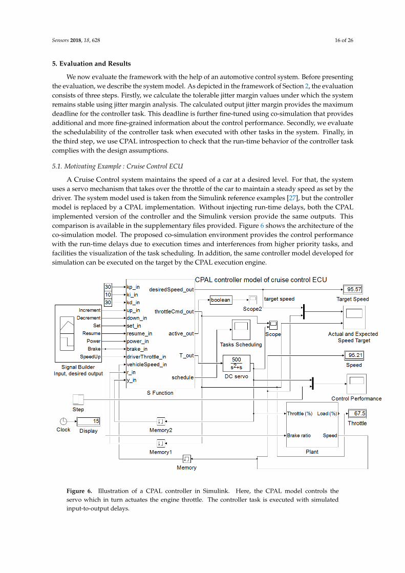
A Cruise Control system maintains the speed of a car at a desired level. For that, the systemuses a servo mechanism that takes over the throttle of the car to maintain a steady speed as set by thedriver. The system model used is taken from the Simulink reference examples [27], but the controllermodel is replaced by a CPAL implementation. Without injecting run-time delays, both the CPALimplemented version of the controller and the Simulink version provide the same outputs. Thiscomparison is available in the supplementary files provided. Figure 6 shows the architecture of theco-simulation model. The proposed co-simulation environment provides the control performancewith the run-time delays due to execution times and interferences from higher priority tasks, andfacilities the visualization of the task scheduling. In addition, the same controller model developed forsimulation can be executed on the target by the CPAL execution engine.

Figure 6. Illustration of a CPAL controller in Simulink. Here, the CPAL model controls theservo which in turn actuates the engine throttle. The controller task is executed with simulatedinput-to-output delays.

Sensors 2018, 18, 628 17 of 26

In our implementation, different tasks and variables are defined within the controller model. Weconsider tasks, namely set point manager, cruise control manager and sensors manager. The label T_out inFigure 6 is the controller tasks’ output which actuates the DC servo mechanism controlling the throttlevalve. We model the DC servo with the transfer function P(s) = 500

(s2+s) . The controller developed relieson a PID control algorithm with proportional gain Kp = 0.96, derivative gain Kd = 0.049, integral gainKi = 0.12 and filter divisor N = 5.0.

5.2. Controller Design

The evaluation of the controller designed consists of two steps, namely the analytical jitter marginmethod and the co-simulation technique.

5.2.1. Step 1. a) Stability Verification Using Jitter Margin Concept

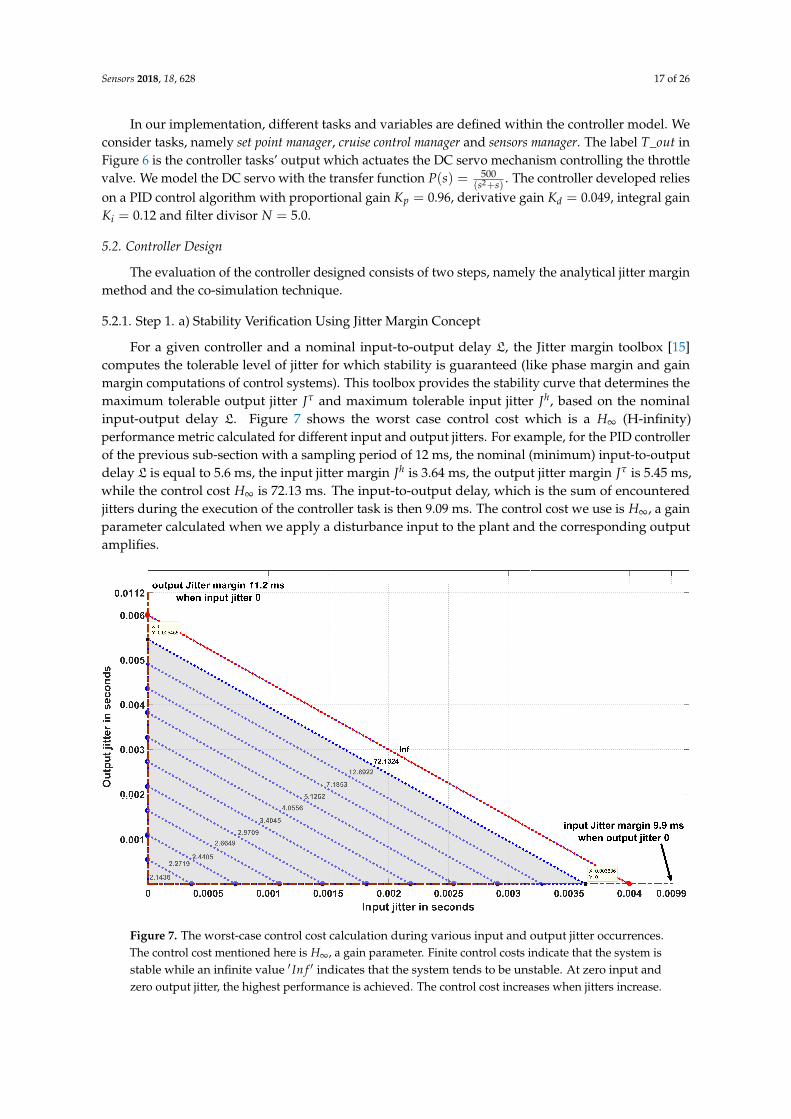
For a given controller and a nominal input-to-output delay L, the Jitter margin toolbox [15]computes the tolerable level of jitter for which stability is guaranteed (like phase margin and gainmargin computations of control systems). This toolbox provides the stability curve that determines themaximum tolerable output jitter Jτ and maximum tolerable input jitter Jh, based on the nominalinput-output delay L. Figure 7 shows the worst case control cost which is a H∞ (H-infinity)performance metric calculated for different input and output jitters. For example, for the PID controllerof the previous sub-section with a sampling period of 12 ms, the nominal (minimum) input-to-outputdelay L is equal to 5.6 ms, the input jitter margin Jh is 3.64 ms, the output jitter margin Jτ is 5.45 ms,while the control cost H∞ is 72.13 ms. The input-to-output delay, which is the sum of encounteredjitters during the execution of the controller task is then 9.09 ms. The control cost we use is H∞, a gainparameter calculated when we apply a disturbance input to the plant and the corresponding outputamplifies.

Figure 7. The worst-case control cost calculation during various input and output jitter occurrences.The control cost mentioned here is H∞, a gain parameter. Finite control costs indicate that the system isstable while an infinite value ′ In f ′ indicates that the system tends to be unstable. At zero input andzero output jitter, the highest performance is achieved. The control cost increases when jitters increase.

Sensors 2018, 18, 628 18 of 26

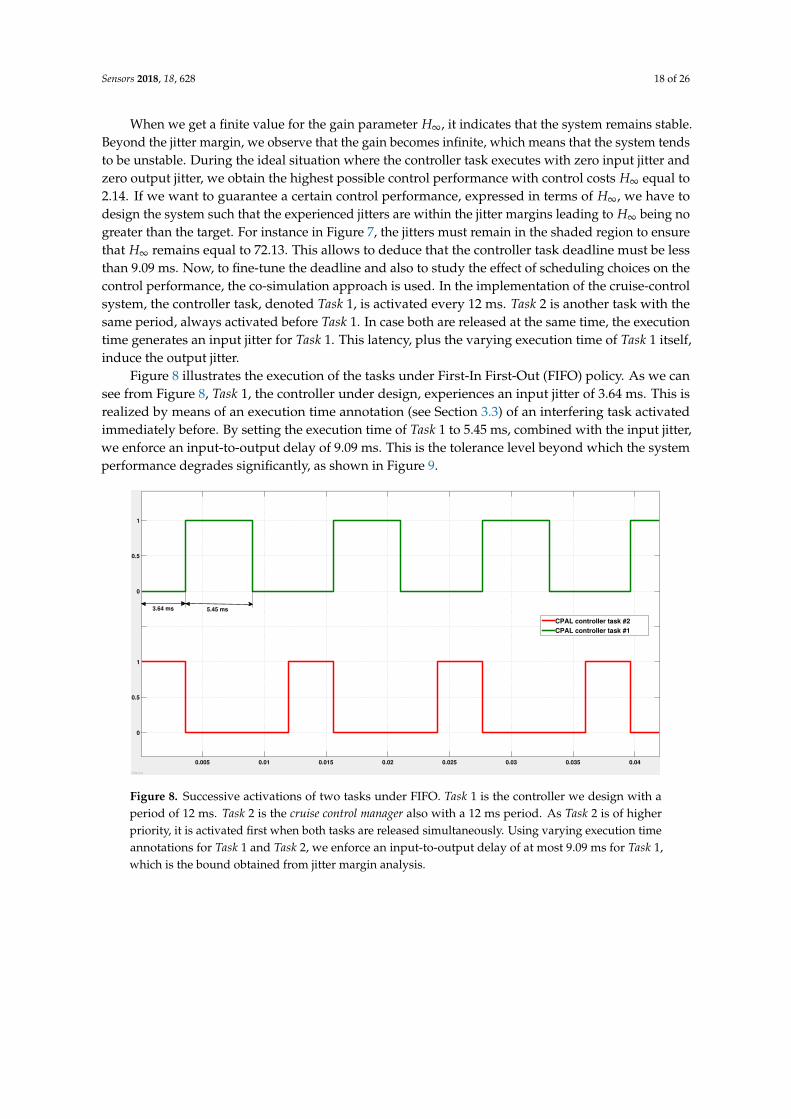
When we get a finite value for the gain parameter H∞, it indicates that the system remains stable.Beyond the jitter margin, we observe that the gain becomes infinite, which means that the system tendsto be unstable. During the ideal situation where the controller task executes with zero input jitter andzero output jitter, we obtain the highest possible control performance with control costs H∞ equal to2.14. If we want to guarantee a certain control performance, expressed in terms of H∞, we have todesign the system such that the experienced jitters are within the jitter margins leading to H∞ being nogreater than the target. For instance in Figure 7, the jitters must remain in the shaded region to ensurethat H∞ remains equal to 72.13. This allows to deduce that the controller task deadline must be lessthan 9.09 ms. Now, to fine-tune the deadline and also to study the effect of scheduling choices on thecontrol performance, the co-simulation approach is used. In the implementation of the cruise-controlsystem, the controller task, denoted Task 1, is activated every 12 ms. Task 2 is another task with thesame period, always activated before Task 1. In case both are released at the same time, the executiontime generates an input jitter for Task 1. This latency, plus the varying execution time of Task 1 itself,induce the output jitter.

Figure 8 illustrates the execution of the tasks under First-In First-Out (FIFO) policy. As we cansee from Figure 8, Task 1, the controller under design, experiences an input jitter of 3.64 ms. This isrealized by means of an execution time annotation (see Section 3.3) of an interfering task activatedimmediately before. By setting the execution time of Task 1 to 5.45 ms, combined with the input jitter,we enforce an input-to-output delay of 9.09 ms. This is the tolerance level beyond which the systemperformance degrades significantly, as shown in Figure 9.

0.005 0.01 0.015 0.02 0.025 0.03 0.035 0.04

0

0.5

1

0

0.5

1

CPAL controller task #2

CPAL controller task #1

Offset=0

5.45 ms3.64 ms

Figure 8. Successive activations of two tasks under FIFO. Task 1 is the controller we design with aperiod of 12 ms. Task 2 is the cruise control manager also with a 12 ms period. As Task 2 is of higherpriority, it is activated first when both tasks are released simultaneously. Using varying execution timeannotations for Task 1 and Task 2, we enforce an input-to-output delay of at most 9.09 ms for Task 1,which is the bound obtained from jitter margin analysis.

Sensors 2018, 18, 628 19 of 26

Time in seconds

0 0.2 0.4 0.6 0.8 1 1.2 1.4 1.6 1.8 2

Un

it s

tep

resp

on

se

0

0.2

0.4

0.6

0.8

1

1.2

Improved step response when deadline islesser than input-to-output delay (# 1)

Unit step signal

Actual step response when deadline is equal to input-to-output delay (# 2)

Step response completely outside

jitter margin

Settling time #2Settling time #1

0.30 s 0.44 s

Figure 9. Control performance using step response for different deadline assignments: equal, less andgreater than the input-to-output delay (resp. blue, green and red curves). The green curve (reducedovershoot one) is obtained with a deadline value equal to 8.2 ms chosen such that the settling timewithin 2% of the steady-state value is less than 0.3 s. When the control task deadline is greater than thejitter margin, logically the system performs poorer with increased oscillations and overshoots.

5.2.2. Step 1. b) Co-Simulation CPAL/Simulink

The co-simulation of CPAL in the Simulink environment serves two purposes: fine-tuning of thedeadline and selection of the scheduling policy. Although the jitter bound derived by jitter marginanalysis helps to assign the deadline, in practice a system designer may want to evaluate the controlperformance with the response to an input elementary signal such as impulse or a step signal. Forthis purpose, we feed an unit step signal in the co-simulation model to study the step response of thesystem. Based on the step response characteristics such as rise time, settling time and overshoot, wecan decide whether a fine tuning of the deadline is necessary. For instance, if the control requirementis to achieve a desired settling time, defined as the time taken to settle within 2% of the steady statevalue, equal to 0.3 s, then the deadline should be no greater than 8.2 ms (versus 0.44 s with a deadlineof 9.09 ms). In our previous work [5], we have exemplified the co-simulation of CPAL in Simulink tostudy the control system performance for different scheduling options.

5.3. Step 2) Software Design

As explained earlier in Section 4.1, the controller model we designed at step 1 is now uploadedon the target platform to estimate a WCET bound. For the specifications of the controller with thesampling period of 12 ms (see Section 5.1), the execution time of the CPAL controller task measuredusing a logic analyzer is 34.4 µs. As explained in Section 4, WCET estimation can also be convenientlyperformed using the CPAL in-built –-stats feature. For the controller task developed, the maximumexecution time value observed is around 200 µs including the scheduler overhead. When there areno preemptions as here, or a bounded number of preemptions, it is possible to include the scheduleroverhead in the WCET of the task. To provision for a safety margin, we consider the execution timealong with the scheduler overhead. We use this WCET and the admissible deadline of 8.2 ms obtainedfrom the previous step to test the schedulability of the system. The schedulability analysis presented in

Sensors 2018, 18, 628 20 of 26

Section 4.3 tells us whether the integrated task set (the controller under design plus the existing taskson the ECU) is feasible or not. In our experimental setup, the task set passes the schedulability test.

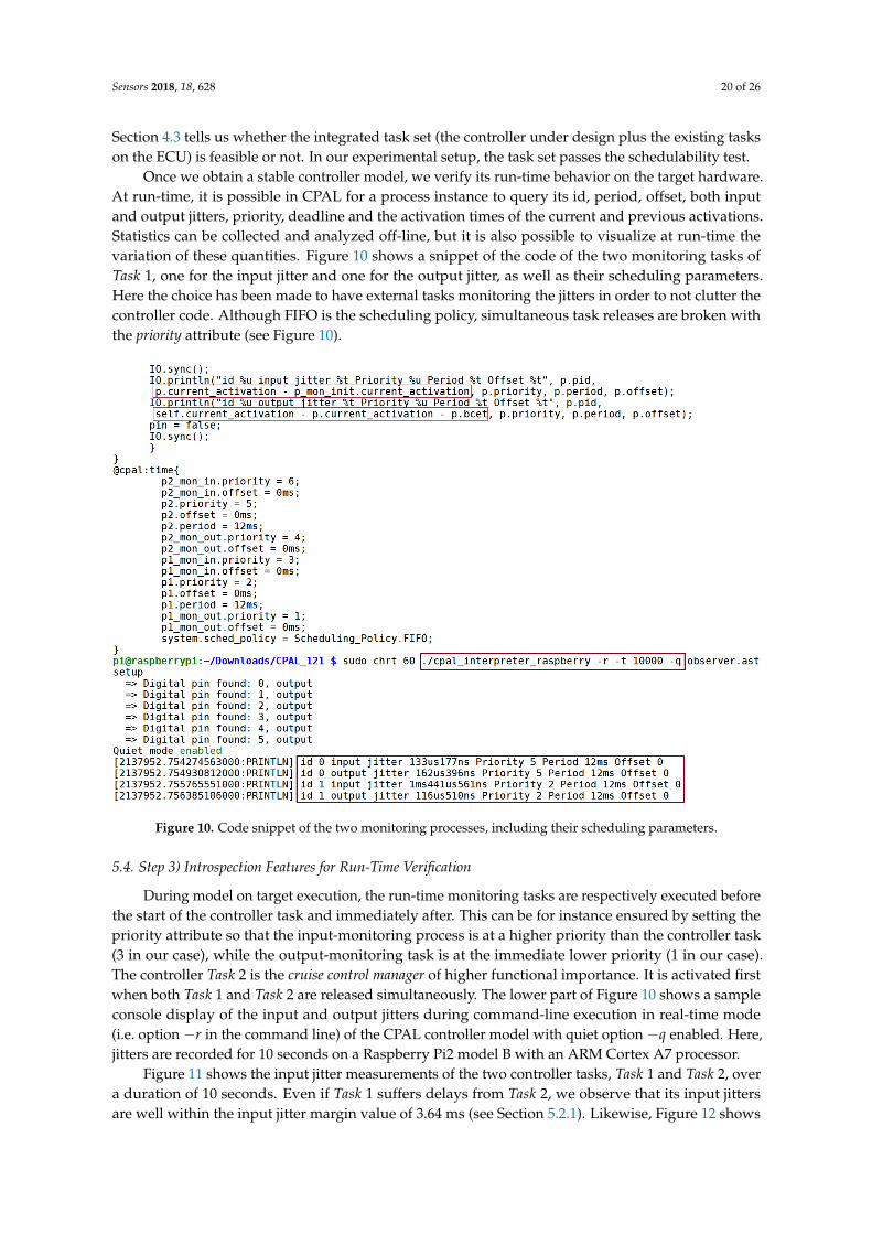
Once we obtain a stable controller model, we verify its run-time behavior on the target hardware.At run-time, it is possible in CPAL for a process instance to query its id, period, offset, both inputand output jitters, priority, deadline and the activation times of the current and previous activations.Statistics can be collected and analyzed off-line, but it is also possible to visualize at run-time thevariation of these quantities. Figure 10 shows a snippet of the code of the two monitoring tasks ofTask 1, one for the input jitter and one for the output jitter, as well as their scheduling parameters.Here the choice has been made to have external tasks monitoring the jitters in order to not clutter thecontroller code. Although FIFO is the scheduling policy, simultaneous task releases are broken withthe priority attribute (see Figure 10).

Figure 10. Code snippet of the two monitoring processes, including their scheduling parameters.

5.4. Step 3) Introspection Features for Run-Time Verification

During model on target execution, the run-time monitoring tasks are respectively executed beforethe start of the controller task and immediately after. This can be for instance ensured by setting thepriority attribute so that the input-monitoring process is at a higher priority than the controller task(3 in our case), while the output-monitoring task is at the immediate lower priority (1 in our case).The controller Task 2 is the cruise control manager of higher functional importance. It is activated firstwhen both Task 1 and Task 2 are released simultaneously. The lower part of Figure 10 shows a sampleconsole display of the input and output jitters during command-line execution in real-time mode(i.e. option −r in the command line) of the CPAL controller model with quiet option −q enabled. Here,jitters are recorded for 10 seconds on a Raspberry Pi2 model B with an ARM Cortex A7 processor.

Figure 11 shows the input jitter measurements of the two controller tasks, Task 1 and Task 2, overa duration of 10 seconds. Even if Task 1 suffers delays from Task 2, we observe that its input jittersare well within the input jitter margin value of 3.64 ms (see Section 5.2.1). Likewise, Figure 12 shows

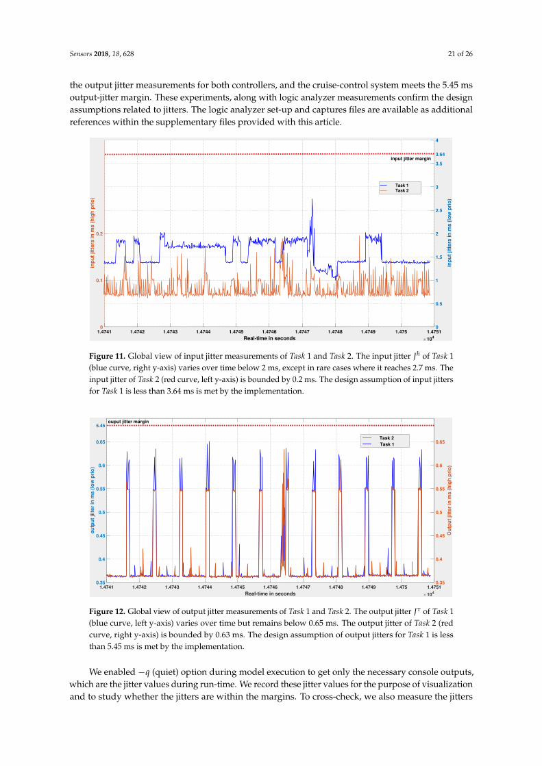
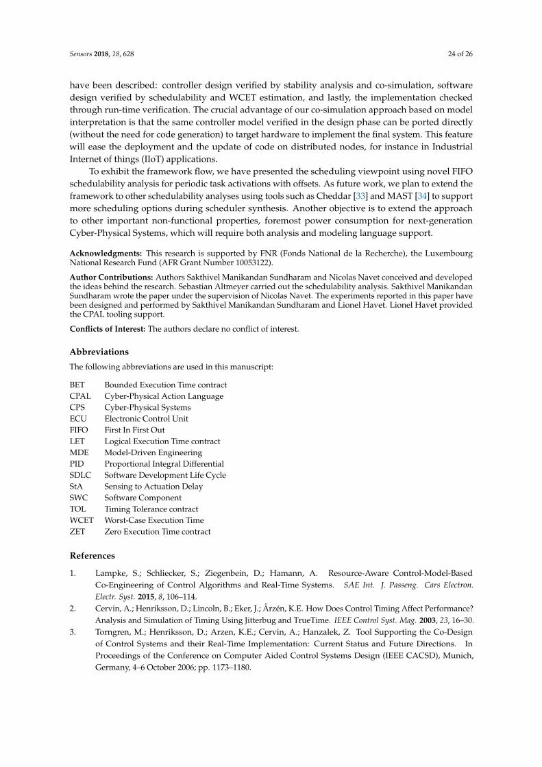
Sensors 2018, 18, 628 21 of 26

the output jitter measurements for both controllers, and the cruise-control system meets the 5.45 msoutput-jitter margin. These experiments, along with logic analyzer measurements confirm the designassumptions related to jitters. The logic analyzer set-up and captures files are available as additionalreferences within the supplementary files provided with this article.

1.4741 1.4742 1.4743 1.4744 1.4745 1.4746 1.4747 1.4748 1.4749 1.475 1.4751

Real-time in seconds ×104

0

0.1

0.2

inp

ut

jitt

ers

in

ms (

hig

h p

rio

)

0

0.5

1

1.5

2

2.5

3

3.5

3.64

4

inp

ut

jitt

ers

in

ms (

low

pri

o)

Task 1

Task 2

input jitter margin

Figure 11. Global view of input jitter measurements of Task 1 and Task 2. The input jitter Jh of Task 1(blue curve, right y-axis) varies over time below 2 ms, except in rare cases where it reaches 2.7 ms. Theinput jitter of Task 2 (red curve, left y-axis) is bounded by 0.2 ms. The design assumption of input jittersfor Task 1 is less than 3.64 ms is met by the implementation.

Real-time in seconds ×104

1.4741 1.4742 1.4743 1.4744 1.4745 1.4746 1.4747 1.4748 1.4749 1.475 1.4751

ou

tpu

t jiit

er

in m

s (

low

pri

o)

0.35

0.4

0.45

0.5

0.55

0.6

0.65

5.45

Ou

tpu

t jitt

er

in m

s (

hig

h p

rio

)

0.35

0.4

0.45

0.5

0.55

0.6

0.65Task 2

Task 1

ouput jitter margin

Figure 12. Global view of output jitter measurements of Task 1 and Task 2. The output jitter Jτ of Task 1(blue curve, left y-axis) varies over time but remains below 0.65 ms. The output jitter of Task 2 (redcurve, right y-axis) is bounded by 0.63 ms. The design assumption of output jitters for Task 1 is lessthan 5.45 ms is met by the implementation.

We enabled −q (quiet) option during model execution to get only the necessary console outputs,which are the jitter values during run-time. We record these jitter values for the purpose of visualizationand to study whether the jitters are within the margins. To cross-check, we also measure the jitters

Sensors 2018, 18, 628 22 of 26

using a logic analyzer with a 100 MHz sampling rate for about 10 seconds, as shown in Figure 13. Fora particular job instance (zoomed portion of the figure), we measure an execution time of 34.58 µsfor controller Task 1 and 25.19 µs for controller Task 2, which both run with a period of 12 ms. Themonitoring processes (input and output) are here to help measure the input jitters, output jitters andinput-to-output delay. We observe that when we do not include the printing of jitter values on theconsole, both input monitor and output monitor tasks (i.e. channels 1, 3 for Task 2 and channels 5, 7 forTask 1) consume less than 4 µs. Note that these monitoring tasks can be removed for the productioncode once the design is finalized to avoid overhead.

Figure 13. The input and output monitoring task activations for two controller tasks captured using alogic analyzer. Both the controller tasks Task 1, Task 2 are activated with a period of 12 ms. Both aredifferent control algorithms which run for an execution time of 34.58 µs and 25.19 µs, respectively atthe highlighted job instant. The monitoring tasks execute only a fraction of the controller’s computationtime, typically less than 4 µs.

6. Related Works

In the literature of computing and control, there have been numerous studies on the effects oftiming irregularities on control performance [2–5]. Cervin et al. coined the term jitter margin in [28],where the authors considered the output jitter margin under which the system still maintains itsstability. In a subsequent work [15], Cervin extended the analysis to account for both the input andoutput jitters on the control performance of linear sampled-data control systems. In this paper, weintegrate this analysis in a tool-supported design flow which guarantees the control performance on agiven execution platform.

A technical contribution needed in this work is a FIFO schedulability analysis for periodic taskswith offsets. Closely related are the results by George and Minet published in [29], who proposed ascheduling analysis for FIFO on a distributed system assuming sporadic task releases, and the resultsby Leontyev and Anderson [30], who developed a tardiness analysis for FIFO scheduling of softreal-time tasks, also assuming a distributed system and sporadic task releases. The two latter worksdid not apply directly to our task model, i.e., periodic task with release offsets.

Sensors 2018, 18, 628 23 of 26

Sangiovanni-Vincentelli et al. discussed various methodologies to address the system designchallenges in [31]. This work highlights the importance of Assume/Guarantee contracts duringcomponent design and explains how a contract can be applied to the design of a water flow controlsystem. Derler et al. proposed in [7] that implicit timing assumptions are made explicit using designcontracts to facilitate the interaction and communication between control and software domains.The authors discussed the support for timing-contracts-based designs using Ptolemy and Simulink.Benveniste et al. proposed in [32] to apply contracts to design methodologies. Importantly, the authorsexplained the mathematical concepts and operations necessary for the contract framework. All theseworks mentioned in this paragraph focused on the fundamental framework for design contracts,such as contract algebra applied in system design, and timing contract visualization in modelingenvironment. In this work, we are concerned with the application of timing tolerance contract inour Model-Based Design flow used to develop control software, thus focusing on scheduling andimplementation issues.

In terms of related design environments, we identify two approaches with associated tools aimingto support control system design considering the influence of scheduling strategies:

• TrueTime: this MATLAB/Simulink-based tool [2] enables the simulation of the temporal behaviorof controller tasks executed on a multitasking real-time kernel. In TrueTime, it is possible toevaluate the performance of control loops subject to the latencies of the implementation. TrueTimeoffers a configurable kernel block, network blocks, protocol-independent send and receive blocksand a battery block. These blocks are Simulink S-functions written in C++. TrueTime is anevent-based simulation using zero-crossing functions. The tasks are used to model the executionof user code and are written as code segments in a MATLAB script or in C++. It models a numberof code statements that are executed sequentially.

• T-Res: this more recent tool [4] is also developed using a set of custom Simulink blocks created tosimulate timing delays dependent on code execution, scheduling of tasks and communicationlatencies, and verifying their impact on the performance of control software. T-Res is inspiredfrom TrueTime and provides a more modular approach to the design of controller modelsenabling to define the controller code independently from the model of the task.

These tools and methods focus on simulation and analysis. They both help the designer to studythe control system performance under the effects of timing delays. The system designer then takessimulation analysis results into account to develop the embedded control algorithms in the next steps.This increases the possibility of distortions between the simulation model and the implementation.An advantage of our co-simulation modelling approach is that the same controller model used toevaluate the control performance during design phase can be re-used directly on the target hardware(in the coding and testing phase) to implement the system. As discussed in our previous work [5,19],the reduced development cycle favors efficient interactions between control and software engineers.The reader is referred to [5] for a review of CPAL in Simulink, TrueTime and T-Res developmentenvironments.

7. Conclusion and Future Work

The timing behavior of control tasks is a critical concern in real-time digital controllers. The delays,such as input jitters, or missed executions due to temporary overload, affect system performanceand are to be accounted for in the design phase. Model-driven engineering has been successful forcapturing the functional requirements during design, but non-functional requirements such as timinghave been traditionally overlooked. This leads to a late verification of controller timing and, in the bestcase, to corrections at a stage when they are costlier. This work is a contribution towards conceivinga design environment for embedded control systems that capture all the necessary functional andnon-functional requirements, while providing analysis, simulation and run-time capabilities.

In this paper, we presented a framework based on timing tolerance contracts which fuses thestability and scheduling viewpoints during controller design. The three steps of the framework

Sensors 2018, 18, 628 24 of 26

have been described: controller design verified by stability analysis and co-simulation, softwaredesign verified by schedulability and WCET estimation, and lastly, the implementation checkedthrough run-time verification. The crucial advantage of our co-simulation approach based on modelinterpretation is that the same controller model verified in the design phase can be ported directly(without the need for code generation) to target hardware to implement the final system. This featurewill ease the deployment and the update of code on distributed nodes, for instance in IndustrialInternet of things (IIoT) applications.

To exhibit the framework flow, we have presented the scheduling viewpoint using novel FIFOschedulability analysis for periodic task activations with offsets. As future work, we plan to extend theframework to other schedulability analyses using tools such as Cheddar [33] and MAST [34] to supportmore scheduling options during scheduler synthesis. Another objective is to extend the approachto other important non-functional properties, foremost power consumption for next-generationCyber-Physical Systems, which will require both analysis and modeling language support.

Acknowledgments: This research is supported by FNR (Fonds National de la Recherche), the LuxembourgNational Research Fund (AFR Grant Number 10053122).

Author Contributions: Authors Sakthivel Manikandan Sundharam and Nicolas Navet conceived and developedthe ideas behind the research. Sebastian Altmeyer carried out the schedulability analysis. Sakthivel ManikandanSundharam wrote the paper under the supervision of Nicolas Navet. The experiments reported in this paper havebeen designed and performed by Sakthivel Manikandan Sundharam and Lionel Havet. Lionel Havet providedthe CPAL tooling support.

Conflicts of Interest: The authors declare no conflict of interest.

Abbreviations

The following abbreviations are used in this manuscript:

BET Bounded Execution Time contractCPAL Cyber-Physical Action LanguageCPS Cyber-Physical SystemsECU Electronic Control UnitFIFO First In First OutLET Logical Execution Time contractMDE Model-Driven EngineeringPID Proportional Integral DifferentialSDLC Software Development Life CycleStA Sensing to Actuation DelaySWC Software ComponentTOL Timing Tolerance contractWCET Worst-Case Execution TimeZET Zero Execution Time contract

References

1. Lampke, S.; Schliecker, S.; Ziegenbein, D.; Hamann, A. Resource-Aware Control-Model-BasedCo-Engineering of Control Algorithms and Real-Time Systems. SAE Int. J. Passeng. Cars Electron.Electr. Syst. 2015, 8, 106–114.

2. Cervin, A.; Henriksson, D.; Lincoln, B.; Eker, J.; Årzén, K.E. How Does Control Timing Affect Performance?Analysis and Simulation of Timing Using Jitterbug and TrueTime. IEEE Control Syst. Mag. 2003, 23, 16–30.

3. Torngren, M.; Henriksson, D.; Arzen, K.E.; Cervin, A.; Hanzalek, Z. Tool Supporting the Co-Designof Control Systems and their Real-Time Implementation: Current Status and Future Directions. InProceedings of the Conference on Computer Aided Control Systems Design (IEEE CACSD), Munich,Germany, 4–6 October 2006; pp. 1173–1180.

Sensors 2018, 18, 628 25 of 26

4. Morelli, M.; Cremona, F.; Di Natale, M. A System-Level Framework for the Evaluation of the PerformanceCost of Scheduling and Communication Delays in Control Systems. In Proceedings of 5th InternationalWorkshop on Analysis Tools and Methodologies for Embedded and Real-Time Systems, Madrid, Spain,8–11 July 2014.

5. Sundharam, S.M.; Havet, L.; Altmeyer, S.; Navet, N. A Model-Based Development Environment forRapid-prototyping of Latency-sensitive Automotive Control Software. In Proceedings of 2016 SixthInternational Symposium on Embedded Computing and System Design (ISED), Patna, India, 15–17December 2016; pp. 228–233.

6. Ziegenbein, D.; Hamann, A. Timing-Aware Control Software Design for Automotive Systems. InProceedings of the 52nd Annual Design Automation Conference, San Francisco, CA, USA, 7–11 June 2015;p. 56.

7. Derler, P.; Lee, E.A.; Törngren, M.; Tripakis, S. Cyber-Physical System Design Contracts. In Proceedings of2013 ACM/IEEE International Conference on Cyber-Physical Systems (ICCPS), Philadelphia, PA, USA,8–11 April 2013; pp. 109–118.

8. Nuzzo, P.; Sangiovanni-Vincentelli, A.L.; Bresolin, D.; Geretti, L.; Villa, T. A Platform-Based DesignMethodology With Contracts and Related Tools for the Design of Cyber-Physical Systems. Proc. IEEE 2015,11, 2104–2132.

9. Kirsch, C.M.; Sokolova, A. The Logical Execution Time Paradigm. In Advances in Real-Time Systems;Springer: Berlin, Germany, 2012; pp. 103–120.

10. Aminifar, A.; Samii, S.; Eles, P.; Peng, Z.; Cervin, A. Designing High-Quality Embedded Control Systemswith Guaranteed Stability. In Proceedings of 2012 IEEE 33rd Real-Time Systems Symposium (RTSS), SanJuan, Puerto Rico, USA, 4–7 December 2012; pp. 283–292.

11. Lincoln, B.; Cervin, A. Jitterbug: A tool for Analysis of Real-Time Control Performance. In Proceedings ofthe 41st IEEE Conference on Decision and Control, Las Vegas, NV, USA, 10–13 December 2002; Volume 2,pp. 1319–1324.

12. Sundharam, S.M.; Altmeyer, S.; Navet, N. Poster Abstract: An Optimizing Framework for Real-TimeScheduling. In Proceedings of 22nd IEEE Real-Time and Embedded Technology and ApplicationsSymposium (RTAS 2016), Vienna, Austria, 11–14 April 2016.

13. Altmeyer, S.; Sundharam, S.M.; Navet, N. The Case for FIFO Real-Time Scheduling; Technical Report, 24935;University of Luxembourg: Luxembourg-city, Luxembourg, 2016.

14. Gerber, R.; Hong, S. Slicing Real-Time Programs for Enhanced Schedulability. ACM Trans. Program. Lang.Syst. 1997, 19, 525–555.

15. Cervin, A. Stability and Worst-Case Performance Analysis of Sampled-Data Control Systems with Inputand Output Jitter. In Proceedings of IEEE American Control Conference (ACC) , Montreal, QC, Canada,27–29 June 2012; pp. 3760–3765.

16. Navet, N.; Fejoz, L.; Havet, L.; Sebastian, A. Lean Model-Driven Development throughModel-interpretation: The CPAL design flow. In Proceedings of 8th European Congress on EmbeddedReal Time Software and Systems (ERTS 2016), Toulouse, France, 27–29 January 2016.

17. The CPAL Programming Language. Available online: https://www.designcps.com/wp-content/uploads/cpal-intro.pdf (accessed on 23 January 2018).

18. Fejoz, L.; Navet, N.; Sundharam, S.M.; Altmeyer, S. Demo Abstract: Applications of the CPAL Languageto Model, Simulate and Program Cyber-Physical Systems. In Proceedings of 2016 IEEE Real-Time andEmbedded Technology and Applications Symposium (RTAS), Vienna, Austria, 11–14 April 2016.

19. Sundharam, S.M.; Altmeyer, S.; Navet, N. Model Interpretation for an AUTOSAR Compliant EngineControl Function. In Proceedings of 7th International Workshop on Analysis Tools and Methodologies forEmbedded and Real-Time Systems (WATERS), Toulouse, France, 5 July 2016.

20. Navet, N.; Fejoz, L. CPAL: High-Level Abstractions for Safe Embedded Systems. In Proceedings of theInternational Workshop on Domain-Specific Modeling, Amsterdam, Netherlands, 30 October 2016; pp.35–41.

21. Wilhelm, R.; Engblom, J.; Ermedahl, A.; Holsti, N.; Thesing, S.; Whalley, D.; Bernat, G.; Ferdinand, C.;Heckmann, R.; Mitra, T.; Mueller, F.; Puaut, I.; Puschner, P.; Staschulat, J.; Stenström, P. The Worst-CaseExecution-Time Problem—Overview of Methods and Survey of Tools. ACM Trans. Embed. Comput. Syst.2008, 7, 36:1–36:53.

Sensors 2018, 18, 628 26 of 26

22. Cazorla, F.J.; Quiñones, E.; Vardanega, T.; Cucu, L.; Triquet, B.; Bernat, G.; Berger, E.; Abella, J.; Wartel, F.;Houston, M.; others. Proartis: Probabilistically Analyzable Real-time Systems. ACM Trans. Embed. Comput.Syst. 2013, 12, 94.

23. Nasri, M.; Davis, R.I.; Brandenburg, B.B. FIFO with Offsets: High Schedulability with Low Overheads.to appear in the Proceedings of 24th IEEE Real-Time and Embedded Technology and ApplicationsSymposium, (RTAS 2018). IEEE, 2018.

24. Pellizzoni, R.; Lipari, G. Feasibility Analysis of Real-Time Periodic Tasks with Offsets. Real Time Syst. 2005,30, 105–128.

25. George, L.; Rivierre, N.; Spuri, M. Preemptive and Non-Preemptive Real-Time Uni-Processor Scheduling.Research Report, 2966; Institut National de Recherche et Informatique et en Automatique (INRIA): Paris,France, 1996.

26. Ripoll, I.; Crespo, A.; Mok, A.K. Improvement in Feasibility Testing for Real-Time Tasks. Real-Time Syts.1996, 11, 19–39.

27. Speed Cruise Control System Using Simulink R© and Stateflow R© - System Model. Available online:https://nl.mathworks.com/help/plccoder/examples/speed-cruise-control-system-using-simulink-and-stateflow.html (accessed on 30 August 2017).

28. Cervin, A.; Lincoln, B.; Eker, J.; Arzén, K.E.; Buttazzo, G. The Jitter Margin and Its Application in theDesign of Real-Time Control Systems. In Proceedings of the 10th International Conference on Real-Timeand Embedded Computing Systems and Applications (Citeseer), Gothenburg, Sweden, 25–27 August 2004;pp. 1–9.

29. George, L.; Minet, P. A FIFO Worst Case Analysis for a Hard Real-Time Distributed Problem withConsistency Constraints. In Proceedings of the 17th International Conference on Distributed ComputingSystems (ICDCS ’97), Baltimore, MD, USA, 27–30 May 1997; pp. 441–448.

30. Leontyev, H.; Anderson, J.H. Tardiness Bounds for FIFO Scheduling on Multiprocessors. In Proceedingsof the 19th Euromicro Conference on Real-Time Systems (ECRTS ’07), Pisa, Italy, 4–6 July 2007;pp. 71–82.

31. Sangiovanni-Vincentelli, A.; Damm, W.; Passerone, R. Taming Dr. Frankenstein: Contract-based Design forCyber-Physical Systems. Euro. J. Contr. 2012, 18, 217–238.

32. Benveniste, A.; Caillaud, B.; Nickovic, D.; Passerone, R.; Raclet, J.B.; Reinkemeier, P.;Sangiovanni-Vincentelli, A.; Damm, W.; Henzinger, T.; Larsen, K.G. Contracts for System Design. ResearchReport, 8147; Rennes, France, 2012.

33. Singhoff, F.; Legrand, J.; Nana, L.; Marcé, L. Cheddar: A Flexible Real-time Scheduling Framework. ACMSIGAda Ada Lett. 2004, 24, 1–8.

34. Harbour, M.G.; García, J.G.; Gutiérrez, J.P.; Moyano, J.D. MAST: Modeling and Analysis Suite for Real-TimeApplications. In Proceedings of 13th IEEE Euromicro Conference on 2001 Real-Time Systems, Delft,Netherlands, 13–15 June 2001; pp. 125–134.

c© 2018 by the authors. Licensee MDPI, Basel, Switzerland. This article is an open accessarticle distributed under the terms and conditions of the Creative Commons Attribution(CC BY) license (http://creativecommons.org/licenses/by/4.0/).