a mixed integer programming model for improving theater

A MIXED INTEGER PROGRAMMING

MODEL FOR IMPROVING THEATER

DISTRIBUTION FORCE FLOW ANALYSIS

THESIS

Micah J. Hafich, Second Lieutenant, USAF

AFIT-ENS-13-M-05

DEPARTMENT OF THE AIR FORCE AIR UNIVERSITY

AIR FORCE INSTITUTE OF TECHNOLOGY

Wright-Patterson Air Force Base, Ohio

APPROVED FOR PUBLIC RELEASE; DISTRIBUTION UNLIMITED.

The views expressed in this thesis are those of the author and do not reflect the official

policy or position of the United States Air Force, Department of Defense, or the United

States Government. This material is declared a work of the U.S. Government and is not

subject to copyright protection in the United States.

AFIT-ENS-13-M-05

A MIXED INTEGER PROGRAMMING MODEL FOR IMPROVING THEATER


THESIS

Presented to the Faculty

Department of Operational Sciences

Graduate School of Engineering and Management

Air Force Institute of Technology

Air University

Air Education and Training Command

In Partial Fulfillment of the Requirements for the

Degree of Master of Science in Operations Research

Micah J. Hafich, BS

Second Lieutenant, USAF

March 2013


AFIT-ENS-13-M-05



Micah J. Hafich, BS

Second Lieutenant, USAF

Approved:

____________________________________ _______________

Dr. Jeffery D. Weir (Advisor) date

____________________________________ _______________

Dr. Raymond R. Hill (Reader) date

iv

AFIT-ENS-13-M-05

Abstract

Obtaining insight into potential vehicle mixtures that will support theater

distribution, the final leg of military distribution, can be a challenging and

time-consuming process for United States Transportation Command (USTRANSCOM)

force flow analysts. The current process of testing numerous different vehicle mixtures

until separate simulation tools demonstrate feasibility is iterative and overly burdensome.

Improving on existing research, a mixed integer programming model was

developed to allocate specific vehicle types to delivery items, or requirements, in a

manner that would minimize both operational costs and late deliveries. This gives insight

into the types and amounts of vehicles necessary for feasible delivery and identifies

possible bottlenecks in the physical network. Further solution post-processing yields

potential vehicle beddowns which can then be used as approximate baselines for further

distribution analysis.

A multimodal, heterogeneous set of vehicles is used to model the pickup and

delivery of requirements within given time windows. To ensure large-scale problems do

not become intractable, precise set notation is utilized within the mixed integer program

to ensure only necessary variables and constraints are generated.

v

Dedication

To my wife, who has supported me from the beginning and was a phenomenal helpmate

throughout the research process.

To my parents, who taught me the value of hard work.

vi

Acknowledgments

I would like to thank Dr. Jeffery Weir for his superb guidance on my thesis

research. I truly appreciate your time, advice, and direction. I am also grateful for your

instruction on VBA and other modeling tools. I wish to thank Dr. Raymond Hill for

serving as a reader and for the introduction to LINGO in OPER 510. Next, I wish to

thank LINDO Systems, particularly Kevin Cunningham, for software assistance with

LINGO. I would also like to thank United States Transportation Command’s Joint

Distribution Process Analysis Center for sponsoring this research and for Mr. Dave

Longhorn’s correspondence throughout the process. Lastly, I would like to thank my

Lord and Savior Jesus Christ for the opportunity to pursue this Master’s degree and for

His blessings throughout this endeavor.

Micah J. Hafich

vii

Table of Contents Page

Abstract .............................................................................................................................. iv

Dedication ........................................................................................................................... v

Acknowledgments.............................................................................................................. vi

List of Figures .................................................................................................................... ix

List of Tables ...................................................................................................................... x

List of Models ................................................................................................................... xii

I. Introduction .................................................................................................................... 1

Background ..................................................................................................................... 1 Research Purpose and Objectives ................................................................................... 7

Organization ................................................................................................................... 9

II. Literature Review ........................................................................................................ 10

Background ................................................................................................................... 10 Airlift Optimization Modeling ...................................................................................... 11

Pickup and Delivery Problem with Time Windows ..................................................... 12 Tabu Search Approaches to Theater Distribution ........................................................ 14

Time-Space Network Approaches ................................................................................ 15 Theater Distribution Model (TDM) .............................................................................. 15 Conclusion .................................................................................................................... 23

III. Methodology .............................................................................................................. 25

Introduction ................................................................................................................... 25

Assumptions ................................................................................................................. 25

Reduced Theater Distribution Model (RTDM) ............................................................ 26 Improved Theater Distribution Model (ITDM) ............................................................ 39 Measuring Vehicle Capacity Utilization ...................................................................... 49

Approximating Beddowns ............................................................................................ 50 Aggregation of Requirements ....................................................................................... 52

Conclusion .................................................................................................................... 53

IV. Implementation and Results ...................................................................................... 54

Implementation ............................................................................................................. 54 Model Testing ............................................................................................................... 55 Determining a Vehicle Beddown .................................................................................. 67 Policy-Driven Solutions ................................................................................................ 68 Aggregation .................................................................................................................. 70 Verification and Validation .......................................................................................... 72

V. Conclusions and Future Research ............................................................................... 75

Conclusions ................................................................................................................... 75 Future Research ............................................................................................................ 77

viii

Appendix A. LINGO 13 Settings File Contents .............................................................. 79

Appendix B. Additional Model Inputs for Test Case 1 and Test Case 2 ......................... 80

Appendix C. TPFDD and Solutions for Test Case 3 ....................................................... 83

Appendix D. Model Coding ............................................................................................. 84

Appendix E. Research Summary Chart ........................................................................... 85

Bibliography ..................................................................................................................... 86

Vita .................................................................................................................................... 88

ix

List of Figures Page

Figure 1. The Three Legs of Joint Military Distribution ................................................... 3

Figure 2. Arbitrary Example Sets .................................................................................... 27

Figure 3. Aggregation of Like Requirements .................................................................. 52

Figure 4. TDM/RTDM Case 1 Solution .......................................................................... 59

Figure 5. ITDM Case 1 Solution...................................................................................... 60

Figure 6. TDM/RTDM Case 2 Solution .......................................................................... 64

Figure 7. ITDM Case 2 Solution...................................................................................... 64

x

List of Tables Page

Table 1. Partial Data from Sample TPFDD ....................................................................... 4

Table 2. TDM Sets ........................................................................................................... 19

Table 3. TDM Parameters ................................................................................................ 20

Table 4. TDM Decision Variables ................................................................................... 20

Table 5. RTDM Basic Sets .............................................................................................. 34

Table 6. RTDM Function Derived Tuple Sets ................................................................. 34

Table 7. RTDM Parameters ............................................................................................. 35

Table 8. RTDM Decision Variables ................................................................................ 35

Table 9. ITDM Basic Sets ................................................................................................ 45

Table 10. ITDM Function Derived Tuple Sets ................................................................ 45

Table 11. ITDM Parameters ............................................................................................ 46

Table 12. ITDM Decision Variables ................................................................................ 46

Table 13. TPFDD for Test Case 1 ................................................................................... 57

Table 14. Test Case 1 Model Results............................................................................... 57

Table 15. Test Case 1 Model Statistics ............................................................................ 58

Table 16. TPFDD for Test Case 2 ................................................................................... 62



Table 19. Vehicle Parameters for Test Case 3 ................................................................. 65



Table 22. Beddowns of Mode Rail, Type DODX vehicles by POD for Test Case 3 ...... 67

xi

Table 23. Vehicle Parameters for Policy-Driven Solutions Example.............................. 69

Table 24. Model Results with Aggregated TPFDD ......................................................... 71

Table 25. Model Statistics with Aggregated TPFDD ...................................................... 71

Table 26. Vehicle Parameters for Test Cases 1 and 2 ...................................................... 80

Table 27. Outloading Parameters for Test Cases 1 and 2 ................................................ 80

Table 28. Unloading Parameters for Test Cases 1 and 2 ................................................. 80

Table 29. Cycle Values for Test Cases 1 and 2 (TDM/RTDM Only) ............................. 81

Table 30. Cycle Values for Test Cases 1 and 2 (ITDM Only) ........................................ 82

xii

List of Models Page

Model 1. Theater Distribution Model (TDM).................................................................. 21

Model 2. Reduced Theater Distribution Model (RTDM) ................................................ 36

Model 3. Improved Theater Distribution Model (ITDM) ................................................ 47

1



I. Introduction

Background

Although varying facets of warfare have changed considerably throughout the

history of combat operations, theater distribution has remained an important concept. In

fact, Alexander the Great successfully conquered much of the known world in the 4th

century B.C. largely because of his proficiency in supplying his army (Engels, 1978).

Theater distribution, a principal component of military logistics, is defined as the flow of

personnel, equipment, and materiel within a given theater as necessitated by the

geographic combatant commander to support theater missions (Joint Chiefs of Staff,

2010). A military force cannot operate in-theater as intended if the war-fighters and their

required provisions are not in the appropriate place at the necessary time. Therefore,

effective theater distribution must be achieved in any military contingency.

The United States (US) military places great emphasis on the superior distribution

of troops and materiel. As such, the core logistic capability of Deployment and

Distribution is an underpinning of the US military’s doctrine on joint logistics. This

doctrinal capability focuses on moving forces, along with their equipment and materiel,

around the globe while maintaining time deadlines dictated by combatant commanders

(Joint Chiefs of Staff, 2008). United States Transportation Command (USTRANSCOM),

2

the unified command responsible for the deployment and distribution of troops and

equipment, supports this logistic capability with sound planning and execution.

Joint military distribution is typically carried out in three specific phases, known

as legs. The first leg, or intracontinental movement, is the movement of forces and cargo

from their initial point of origin to a Port of Embarkation (POE). The first leg typically

remains within the United States, with troops and cargo departing from unit bases to a

POE for further movement. The second leg, intertheater movement, involves movement

from a POE to an in-theater Port of Debarkation (POD). This leg usually entails the

movement of forces and goods from the United States to a specific theater of operations.

The final leg, known as intratheater movement or theater distribution, occurs when

personnel and materiel are moved from an in-theater POD to their final delivery

destination, or Point of Need, within the operating area (Joint Chiefs of Staff, 2010).

This final leg occurs entirely within the operational theater. Throughout the distribution

process, ports (both PODs and POEs) may be either aerial ports or sea ports. An example

of how the three legs of distribution work together to deliver goods from origin to theater

is shown below in Figure 1.

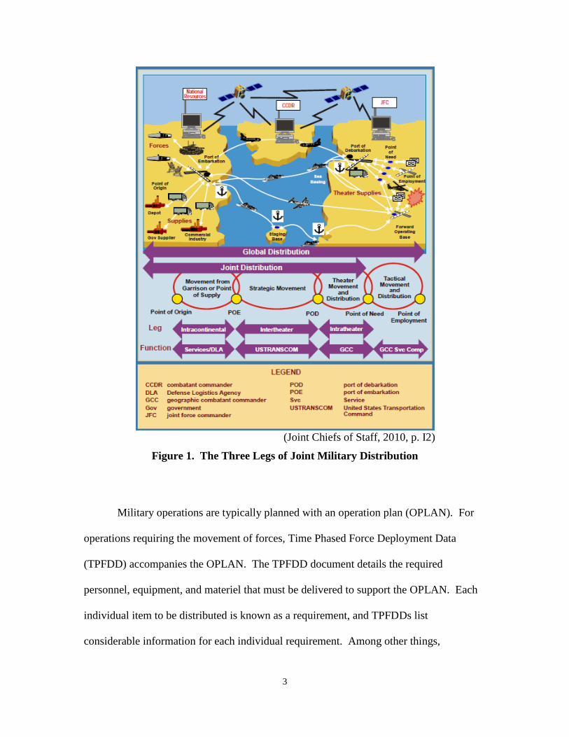
3

(Joint Chiefs of Staff, 2010, p. I2)

Figure 1. The Three Legs of Joint Military Distribution

Military operations are typically planned with an operation plan (OPLAN). For

operations requiring the movement of forces, Time Phased Force Deployment Data

(TPFDD) accompanies the OPLAN. The TPFDD document details the required

personnel, equipment, and materiel that must be delivered to support the OPLAN. Each

individual item to be distributed is known as a requirement, and TPFDDs list

considerable information for each individual requirement. Among other things,

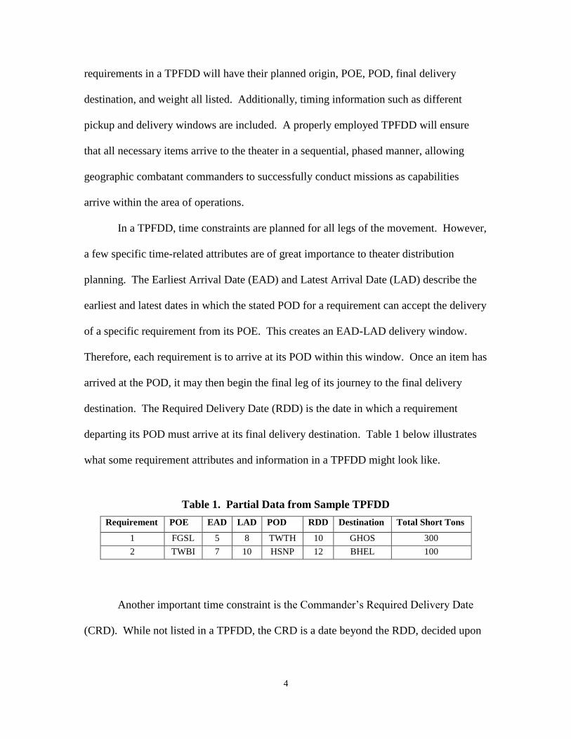
4

requirements in a TPFDD will have their planned origin, POE, POD, final delivery

destination, and weight all listed. Additionally, timing information such as different

pickup and delivery windows are included. A properly employed TPFDD will ensure

that all necessary items arrive to the theater in a sequential, phased manner, allowing

geographic combatant commanders to successfully conduct missions as capabilities

arrive within the area of operations.

In a TPFDD, time constraints are planned for all legs of the movement. However,

a few specific time-related attributes are of great importance to theater distribution

planning. The Earliest Arrival Date (EAD) and Latest Arrival Date (LAD) describe the

earliest and latest dates in which the stated POD for a requirement can accept the delivery

of a specific requirement from its POE. This creates an EAD-LAD delivery window.

Therefore, each requirement is to arrive at its POD within this window. Once an item has

arrived at the POD, it may then begin the final leg of its journey to the final delivery

destination. The Required Delivery Date (RDD) is the date in which a requirement

departing its POD must arrive at its final delivery destination. Table 1 below illustrates

what some requirement attributes and information in a TPFDD might look like.

Table 1. Partial Data from Sample TPFDD

Requirement POE EAD LAD POD RDD Destination Total Short Tons

1 FGSL 5 8 TWTH 10 GHOS 300

2 TWBI 7 10 HSNP 12 BHEL 100

Another important time constraint is the Commander’s Required Delivery Date

(CRD). While not listed in a TPFDD, the CRD is a date beyond the RDD, decided upon

5

by the geographic combatant commander, in which a requirement must have arrived at

the final delivery destination. Therefore, while undesirable, delivery after the RDD but

on or before the CRD can be allowed in modeling to assess late impacts. (Joint Chiefs of

Staff, 2011a).

As part of distribution planning, and in order to ensure successful future military

movements, USTRANSCOM holds recurring force flow conferences. At these

conferences, proposed OPLANs and accompanying TPFDDs are tested against logistical

capabilities to determine the feasibility of planned actions. Analysts and planners must

determine whether or not requirements listed in an OPLAN’s TPFDD can be realistically

delivered based upon the planned delivery network, assigned transportation vehicles, and

the timelines for movements. If analysis shows that the transportation of the required

equipment and materiel needed to begin and sustain operations cannot be conducted in a

feasible manner, an iterative process of refining the OPLAN and TPFDD is conducted

until a satisfactory and feasible operation plan is established (Joint Chiefs of Staff, 2010).

While USTRANSCOM force flow conferences may examine all three legs of

military distribution during their analysis, particular attention must be given to theater

distribution, the intratheater movement between PODs and final destinations. Firstly,

theater distribution normally requires a beddown of vehicles within the theater in order to

sustain delivery to the final destination. Thus, determining how to allocate requirements

to vehicles and deciding which vehicles to position at theater locations to support theater

distribution can be a challenging task. Secondly, the theater distribution phase is crucial

to ensuring war-fighters receive their goods and materiel on time. Timeliness is

imperative in this last leg as late deliveries could negatively impact military operations

6

and potentially harm US forces. Movement requirements shipped on-time to the POD are

useless to troops in combat if they do not also arrive on-time to the theater locations.

Thus, it is imperative that appropriate analysis is conducted on theater distribution.

At USTRANSCOM force flow conferences various mobility simulation tools are

used to find feasible delivery options by examining the transportation networks and assets

under consideration. An internal research paper authored by Longhorn & Kovich (2012)

of USTRANSCOM points out that while these simulation models are helpful in

conducting theater distribution analysis, they only describe limitations to theater

distribution without prescribing any potential fixes. In other words, the simulation tools

report only on the feasibility or infeasibility of specific transportation plans based upon

the constraints of the specific network under consideration and the transportation assets

selected to be utilized within the simulation. Once limitations or infeasibilities are found,

no current tool exists to describe an appropriate vehicle mixture that will allow the

operation to then become feasible. In fact, it may take many time-consuming “trial and

error” runs with differing transportation vehicle mixtures until one that supports feasible

movement is found.

To address this, Longhorn & Kovich (2012) propose an integer programming

optimization formulation, known throughout this thesis as the Theater Distribution Model

(TDM). The TDM, discussed thoroughly in Chapter II, would prescribe, before

simulation of the theater distribution phase, a specific multimodal vehicle mixture that is

needed to successfully deliver the materiel for a specific operation. Once determined, the

specific vehicle mixtures would be used as input in the simulation tools as analysts

continue with distribution analysis. Because the vehicle mixture solutions drawn from

7

the TDM would demonstrate sufficient transportation assets for the requirements, they

should yield feasible transportation plans. Thus, analysts can avoid the iterative, timely

process of checking for feasibility and adapting as necessary. Furthermore, by making

cost changes in the optimization models, analysts can also compare how different policy

changes would impact theater distribution efforts. (Interested readers should contact Dr.

Jeff Weir, AFIT/ENS, at [email protected] for information on obtaining the

Longhorn & Kovich internal research paper).

Research Purpose and Objectives

The purpose of this research is to improve contingency planning capabilities at

USTRANSCOM, specifically for force flow analysis of theater distribution. At present,

analysts at USTRANSCOM have no functioning optimization models that dictate, for a

given operation, a feasible number of vehicles needed to conduct theater distribution in

an on-time, least-cost method. Currently, planners initially select a vehicle mixture that

may or may not yield feasible transportation after analysis. Next, simulation tools are run

to examine whether or not that particular predetermined vehicle mixture will allow for

feasible flow within the network. If the analysis shows infeasibility, another vehicle

mixture is tested.

Because the simulations are descriptive in nature, they do not give insight into

what types of vehicle mixtures would provide for feasible transportation and because of

this, potential vehicle mixtures are often selected via “trial and error”. However, even if

a particular vehicle mixture is found to yield feasible transportation within the network,

there is certainly no guarantee that the vehicle mixture is even remotely optimal in terms

of costs. This iterative technique of finding vehicle mixtures can be extremely time

mailto:[email protected]

8

consuming, requiring hours of simulation every time a new vehicle mixture is tested for

feasible transportation. The objective of the proposed TDM is to find on-time, least-cost

delivery options for all requirements within the TPFDD, detailing on what days different

types of vehicles should be available for transportation. However, the TDM has yet to be

thoroughly tested.

The first objective of this research is to test the proposed TDM and determine if it

is capable of finding solutions to large-scale problems, such as those engendered with

TPFDDs for US military contingencies. A typical TPFDD may easily contain thousands

of movement requirements. Thus, it is important to ensure that any proposed model is

computationally efficient as problems can grow rapidly in size.

The second objective of this research is to determine if the TDM optimization

model adequately matches reality. That is, the validity of the model must be inspected to

ensure that it appropriately finds the vehicle mixture necessary for requirements in an

on-time, least-cost method.

Thirdly, this research will examine possible changes to the formulation of the

model. In particular, the process by which vehicles are allocated to requirements will be

investigated.

Lastly, the research will attempt to construct approximate vehicle beddowns that

would be necessary at each POD based upon the model solutions. Beddowns may be

helpful to analysts as they attempt to model the theater distribution portion of movements

with simulation tools.

With these objectives in mind, this research intends to save USTRANSCOM

countless hours of analysis and planning at their force flow conferences. A functional

9

optimization model for force flow analysis will allow operational planners to quickly find

feasible vehicle mixtures for intratheater transportation needs rather than going through

multiple stages of guesswork, followed by hours of simulation, when selecting a vehicle

mixture for successful theater distribution in a planned contingency operation.

Furthermore, in addition to reducing the man-hours required to conduct the

planning, testing, and analysis of OPLANs/TPFDDs, an optimization model would allow

analysts to explore different feasible vehicle mixtures by changing model inputs as a

demonstration of different policy decisions or other driving forces. Through this

research, improved efficiency in planning of theater distribution will help ensure

war-fighters are given the materiel and equipment they need in an on-time and least-cost

manner.

Organization

The remainder of this thesis contains four additional chapters. Chapter II

provides a literature review of airlift optimization modeling, the Pickup and Delivery

Problem with Time Windows, and other relevant models focused on distribution.

Additionally, the proposed TDM is introduced and explained in detail. In Chapter III, the

methodology utilized in this research is discussed. In particular, a reduced-size, mixed

integer programming solution method is developed. Chapter IV shows the

implementation of the methodology and demonstrates improvements over the TDM.

Chapter V offers concluding remarks and discusses how this research might be extended

with further work.

10

II. Literature Review

This chapter will provide a review of relevant literature, focusing mainly on

distribution-related models. The research mentioned herein is not entirely exhaustive, but

gives the reader a general understanding of past efforts in areas such as airlift

optimization modeling, the Pickup and Delivery Problem with Time Windows, and

specific Tabu Search approaches to theater distribution. Additionally, great detail is

given on the Theater Distribution Model, or TDM. This model, developed for the

purpose of force flow analysis, was the basis of this thesis research.

Background

The US Military utilizes a number of simulation tools to assist in mobility

planning. Interested readers are directed to McKinzie & Barnes (2004) for a review of

some of these models. However, as discussed by Longhorn & Kovich (2012), these

models tend to describe rather than prescribe various aspects of theater distribution.

While various optimization techniques have been applied to military transportation

problems throughout the years, many of them are aimed at the specific routing and

scheduling of individual vehicles. However, force flow analysts are not concerned with

creating individual routes for vehicles.

Force flow analysis is strictly for planning purposes, in which analysts attempt to

judge the feasibility of future transportation plans and adapt plans when necessary.

Furthermore, combat is a dynamic environment in which many aspects cannot be planned

for exactly because scenarios often can, and do, change instantly. For example, physical

factors such as terrain, weather, and the impacts of friendly and enemy forces greatly

11

affect operations and sustainment (Joint Chiefs of Staff, 2011b). For these reasons, the

creation of individual vehicle routes and schedules is neither necessary nor desired for

force flow analysis. Instead, analysts simply desire a baseline vehicle mixture that will

successfully support distribution operations. This chapter will offer a review of

distribution modeling efforts as well as specific mathematical approaches to closely

related problems such as the Pickup and Delivery Problem with Time Windows.

Airlift Optimization Modeling

Early optimization efforts on military distribution often focused on airlift

capabilities. Rappoport, Levy, Toussaint, & Golden (1994) developed a transportation

problem formulation to be utilized in airlift planning for Military Airlift Command, the

predecessor to the US Air Force’s Air Mobility Command (AMC). The model was

utilized to assign differing airlift vehicle types, such as bulk or outsize, and shipment

days to specific requirements. Then, once these matches were made, the results were

preprocessed and then placed into a heuristic routing and scheduling procedure known as

the Airlift Planning Algorithm (APA). The model, set up as a linear programming

transportation problem, minimized the costs of assigning capacity to different

requirements. While the model matches vehicle types to movements as a preprocessor to

further modeling, the transportation model does not dictate the number of vehicles

needed to sustain flow within the network.

Shortest path techniques have also been applied to AMC aircraft routing. Rink,

Rodin, Sundarapandian, & Redfern (1999) applied a double-sweep algorithm to find the

k - shortest paths between each onload location and offload location given in a TPFDD.

However, the time factor (i.e. avoiding lateness) is not considered in this model. Shortest

12

path methods can be a hindrance to successful analysis. Due to certain policy decisions

regarding concerns like safety or enemy in the area, a shortest path may not be the best

path. Additionally, shortest paths are not guaranteed to have enough outloading and

unloading resources to support distribution.

Rosenthal et al. (1997) discuss the use of THRUPUT II, a model developed at the

Naval Post Graduate School, in order to model the entire transportation network. Linear

programming is used to yield on-time throughput of both cargo and passengers. That is,

given the inputs of units to be moved, airfields available, aircraft available, and routes

available, the model provides routes and mission start times for aircraft within the model.

All airlift models have an inherent drawback for use in theater distribution

analysis because they fail to consider movement amongst other modes of transportation,

such as rail or road. Thus, the effects and tradeoffs between different modes cannot be

properly assessed. In theater distribution, multiple modes are usually available and thus

multimodal modeling is important.

Pickup and Delivery Problem with Time Windows

In theater distribution, requirements are to be picked up at their respective POD

and then delivered to their in-theater destination. A TPFDD will dictate what the time

windows for both the pick-up at the POD and delivery at the Destination are. Because of

the time windows on both the pickup and delivery, this problem is related to an

optimization problem known as the Pickup and Delivery Problem with Time Windows

(PDPTW). The PDPTW involves transportation requests that have both a pickup and

delivery location along with time windows in which the pickup and delivery must occur.

Solutions to the PDPTW yield optimal routes for vehicles in which demand is met within

13

the appropriate time windows while meeting capacity and precedence constraints

(Dumas, Desrosiers, & Soumis, 1991).

Dumas et al. (1991) offer a PDPTW mathematical formulation that utilizes a

homogenous fleet of vehicles and is solved utilizing column generation with a shortest

path subproblem. Many other solution attempts to the PDPTW have been developed,

such as the Reactive Tabu Search method employed by Nanry & Barnes (2000).

Furthermore, Baldacci, Bartolini, & Mingozzi (2011) utilize a set partitioning

formulation to solve the PDPTW. Readers interested in exploring the different

formulations and applications of the PDPTW may review Cordeau, Laporte, Potvin, &

Savelsbergh (2007).

Because the US military has numerous vehicle types in their inventory, the

PDPTW with a homogenous fleet is not a particularly useful model. However, pickup

and delivery models utilizing multiple vehicle types have been studied. Lu & Dessouky

(2004) developed an exact algorithm for solving the multiple vehicle pickup and delivery

problem (MVPDP), which may include time windows. Their integer programming

formulation allows for multiple heterogeneous vehicles. Many heuristic solution

methods to the MVPDP have also been developed and interested readers may reference

Savelsbergh & Sol (1995). Xu, Chen, Rajagopal, & Arunapuram (2003) developed a

Practical Pickup and Delivery Problem (PPDP) that extends the PDPTW to include, not

only multiple vehicle types, but many additional considerations such as multiple time

windows, travel time restrictions, and compatibility constraints.

It is important to point out that the PDPTW typically involves an assumption that

a set number of vehicles are located at depots from which vehicles begin their routes.

14

However, in theater distribution, vehicles are typically not centrally located at some depot

where they are then scheduled and routed for missions. Instead, transportation assets are

typically delivered into the theater of operations. In fact, a goal of force flow analysis is

to determine how many vehicles of each type need to be located at different PODs to

begin supporting transportation requirements.

Tabu Search Approaches to Theater Distribution

Tabu Search approaches have recently been applied specifically to theater

distribution problems. Crino, Moore, Barnes, & Nanry (2004) utilized Group Theoretic

Tabu Search in order to solve the Theater Distribution Vehicle Routing and Scheduling

Problem. This is a powerful approach which prescribes the routing and scheduling of

multimodal theater transportation assets at the individual vehicle level in order to provide

time-definite delivery of cargo. Likewise, Burks, Moore, Barnes, & Bell (2010) utilized

Adaptive Tabu Search in an attempt to solve the theater distribution problem. This model

focuses on solving two separate problems simultaneously. It solves both the Location

Routing Problem and the Pickup and Delivery Problem with Time Windows to optimally

choose locations of depots and supply points as well as the specific routes of vehicles

while satisfying all demand requirements. As with many other models discussed in this

chapter, these models prescribe individual vehicle routes and schedules.

While these Tabu Search approaches optimize time-definite delivery and allow

multiple modes to be utilized within the transportation network, the models are of such

high-fidelity that they are of little use in force flow analysis. Because too many factors

could change an individual vehicle’s route under combat scenarios, a general

approximating solution approach, at the aggregate vehicle level, is preferred for force

15

flow analysis. Thus, while a model employing Tabu Search may provide practical results

for a day-to-day outlook on theater distribution operations, these models are not

particularly insightful for force flow analysis, where a generalized solution that provides

baseline estimates for necessary vehicles is more favorable (Longhorn & Kovich, 2012).

Time-Space Network Approaches

In order to model disaster relief operations Haghani & Oh (1996) developed a

multicommodity, multimodal network flow model that finds the optimal use of different

modes in a network to meet commodity and time requirements. To do this, a time-space

network is utilized, which means that nodes in the network represent not only the

physical locations of supply and demand, but also moments in time. Thus, time can be

captured as flow occurs through the network. A time-space network technique is also

utilized by Clark, Barnhart, & Kolitz (2004) to model the distribution of US Army

Munitions, where ammunition and ship movements are scheduled within the distribution

system.

Theater Distribution Model (TDM)

TDM Overview.

To determine an appropriate mixture of vehicles necessary to conduct theater

distribution for specific contingencies, Longhorn & Kovich (2012) proposed a pure

integer programming model. The Theater Distribution Model (TDM) attempts to find an

optimum allocation of requirements to vehicles such that time-definite delivery occurs in

a least-cost manner. Unlike other distribution models, the TDM does not specify routes

and schedules for individual vehicles. As previously discussed, those sorts of high-

fidelity models are impractical for force flow analysis. Instead, the TDM answers

16

questions such as when, where, what type, and how many when discussing vehicles

needed to conduct theater distribution subject to physical network constraints.

In the TDM, users must select which modes of transportation and vehicle types

they wish to enter into the model. Selected modes form the set M . The individual

Modes m M will typically contain all or some elements of the set {Air, Road, Rail}.

Vehicle Types are selected by the user to form a set of vehicle Types K . Each vehicle

Type k K is a specific vehicle (e.g. C-17) of a single Mode m , and has two input

parameters associated with it. The first parameter is the daily cost of utilizing vehicle

Type k , kb . This cost could be financial in nature, but it may also be utilized as an

arbitrary cost in order to analyze the impact certain policy decisions have upon solutions.

The second parameter is kp , the average payload (measured in short tons) of a vehicle

of Type k .

The TDM draws much data for use in analysis from the TPFDD that is associated

with the theater distribution plan under analysis. The TPFDD under consideration will

list maxn separate movement requirements. Thus, the set {1,... }maxN n contains a

unique identifier for all movement requirements in the TPFDD. Each movement

Requirement n N has associated data with it such as the specific requirement’s POD,

Destination, EAD, RDD, and total weight. The set I contains all PODs i included in

the TPFDD requirements while the set J contains all Destinations j . Each

movement Requirement n , to be delivered from POD i to Destination j , has a

requirement weight nijr which is measured in short tons. Within the model, it is

17

assumed that all requirements are standard cargo requirements. Passenger requirements

and any potential restrictions on outsize or oversize cargo are ignored.

The variable nad describes the day in which Requirement n arrives at its stated

POD. The TDM assumes that a requirement may not ship from its POD until the day

immediately following its arrival at the POD. In other words, the first day in which

Requirement n can deliver from its POD to its Destination would be the day 1nad .

The variable nrd indicates the Required Delivery Date, or RDD, at the Destination for

each Requirement n . Any requirement arriving after the RDD is considered late.

Analysts and commanders may work together to determine how late a requirement may

be for analysis. Each Requirement n may be given nqd extension days in order to be

delivered. Delivering on an extension day is allowable, but the movement will be

denoted as late and a penalty, g , will be assessed per vehicle for each day late. The

value of g is user-defined.

The TDM does not allow requirements to be delivered beyond their RDD plus

any input extension days. Mathematically, this means that each requirement n must be

picked up and delivered within the time window beginning at day 1nad and ending at

n nrd qd . Thus, the Days utilized within the model range from min 1nn N

ad

to

max n nn N

rd qd

. The set V describes this set of Days v for delivery, spanning the

absolute earliest possible day of requirement delivery and the absolute latest possible

delivery day based upon information located in the TPFDD.

18

Physical limitations of the distribution network are captured in the TDM with

restrictions on the number of vehicles which may be outloaded at PODs and unloaded at

Destinations within a given day. Characteristics such as space and manning may impact

the amount of vehicles that may pass through a POD or Destination daily. The TDM

assumes that these outloading and unloading limits are not based upon specific vehicle

Types, only vehicle Modes. In the model, imvo describes the maximum number of Mode

m vehicles that can be outloaded at POD i on Day v of the operation. Likewise,

jmvu describes the maximum number of Mode m vehicles that can be unloaded at

Destination j on Day v . If a certain POD or Destination does not support the

movement of a certain Mode, then the associated parameters imvo , or jmvu

respectively, would have a value of zero. Typically, subject matter experts can provide

these parameters.

The TDM assumes that a vehicle type assigned to a requirement will transport

directly from the POD to Destination, and back and forth as necessary, until the entire

requirement has completely been delivered. Thus, the model requires data on how many

direct trips may be completed in a single day. The parameter nijmkw details the

approximate number of daily cycles that can be completed by a Mode m , Type k

vehicle delivering Requirement n from POD i to Destination j . These

approximate cycle values must be calculated before being input into the model and

should take into account outloading and unloading times as well as distance between

locations and vehicle speeds. Interested readers are encouraged to reference Longhorn &

Kovich (2012) to see their cycle calculations.

19

The decision variable of the TDM is nijmkvx , which describes the number of

vehicles of Mode m , Type k that are required on Day v to deliver Requirement n

from POD i to Destination j . Thus, the decision variables provide much pertinent

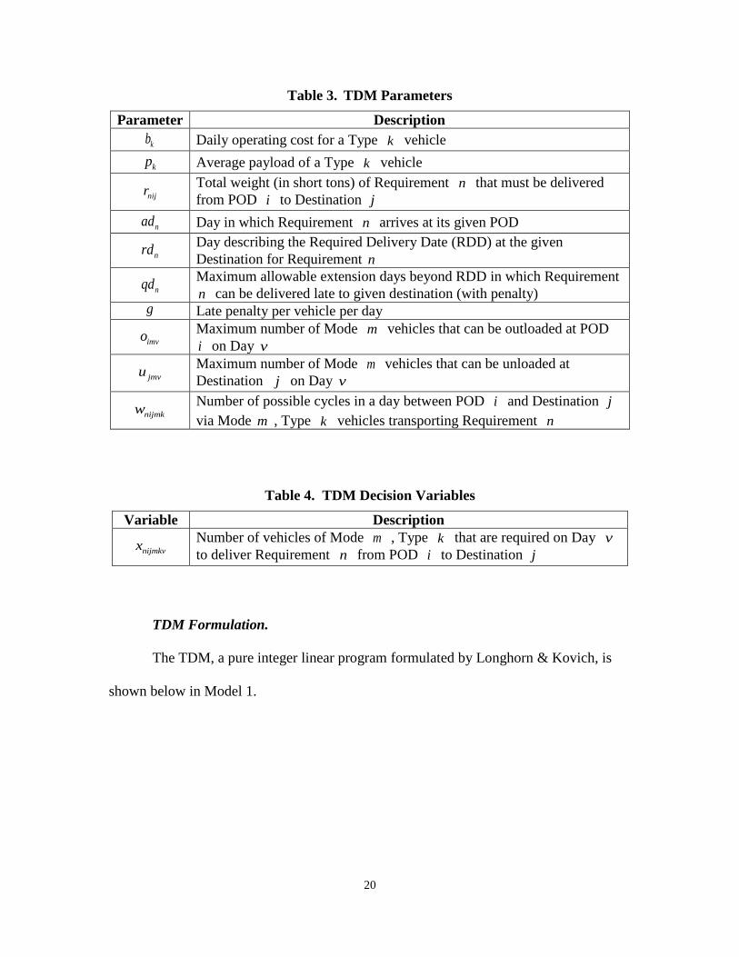
information when assessing a vehicle mixture solution output. Table 2 - Table 4 below

summarize the sets, parameters, and decision variables utilized in the TDM’s pure integer

programming formulation.

Table 2. TDM Sets

Set Description

N Set of all Movement Requirements n

I Set of all PODs i

J Set of all Destinations j

M Set of all vehicle Modes m

K Set of all vehicle Types k

V Set of all possible delivery Days v

20

Table 3. TDM Parameters

Parameter Description

kb Daily operating cost for a Type k vehicle

kp Average payload of a Type k vehicle

nijr Total weight (in short tons) of Requirement n that must be delivered

from POD i to Destination j

nad Day in which Requirement n arrives at its given POD

nrd Day describing the Required Delivery Date (RDD) at the given

Destination for Requirement n

nqd Maximum allowable extension days beyond RDD in which Requirement

n can be delivered late to given destination (with penalty) g Late penalty per vehicle per day

imvo Maximum number of Mode m vehicles that can be outloaded at POD

i on Day v

jmvu Maximum number of Mode m vehicles that can be unloaded at

Destination j on Day v

nijmkw Number of possible cycles in a day between POD i and Destination j

via Mode m , Type k vehicles transporting Requirement n

Table 4. TDM Decision Variables

Variable Description

nijmkvx Number of vehicles of Mode m , Type k that are required on Day v

to deliver Requirement n from POD i to Destination j

TDM Formulation.

The TDM, a pure integer linear program formulated by Longhorn & Kovich, is

shown below in Model 1.

21

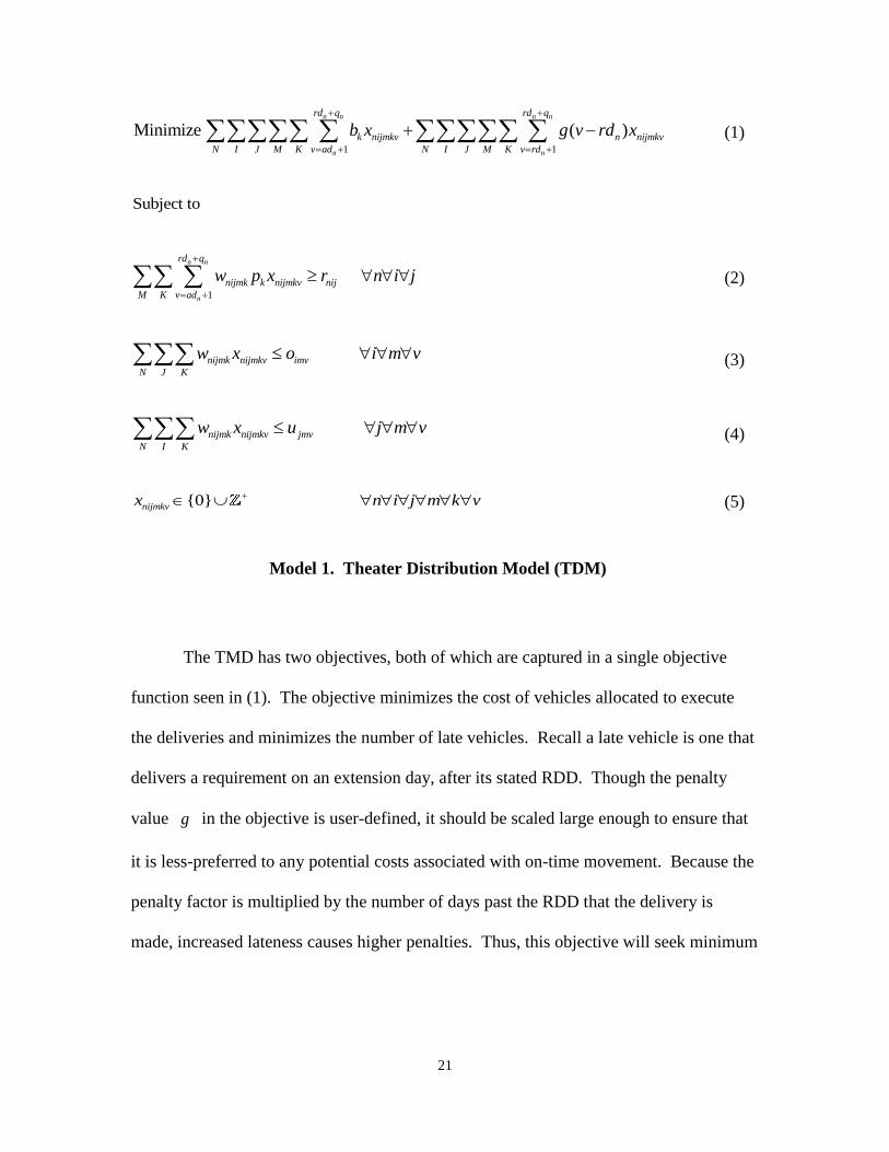
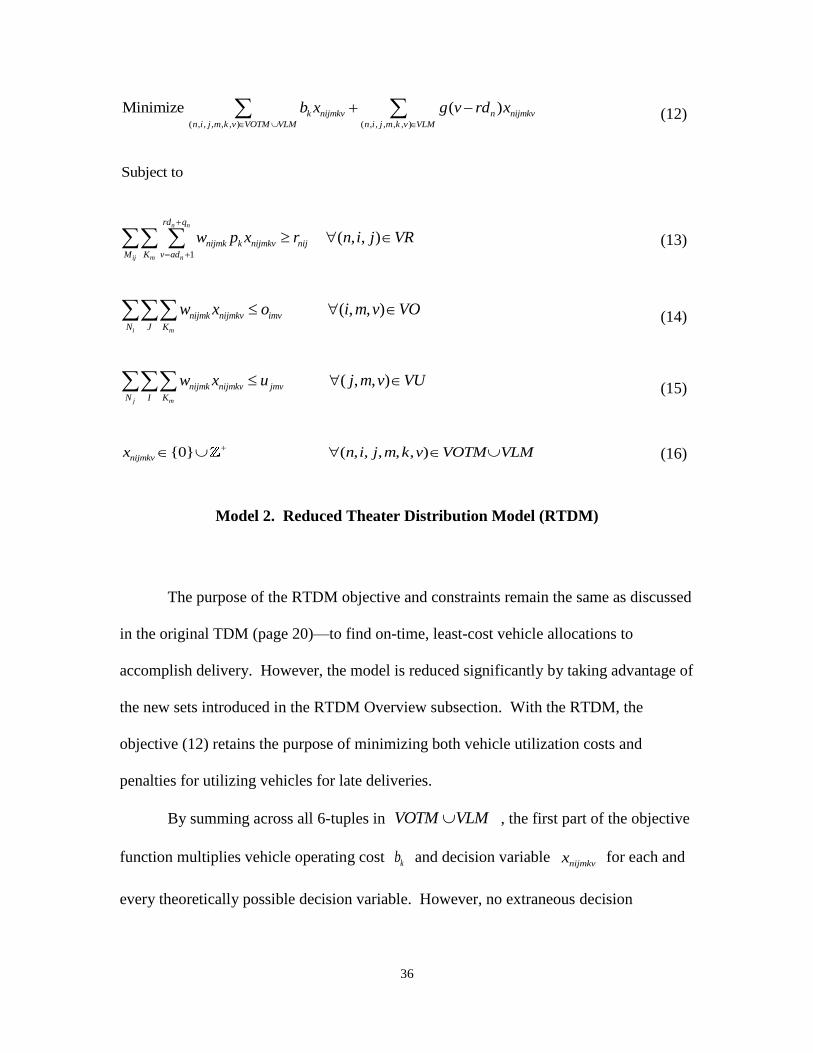
1 1

Minimize ( )n n n n

n n

rd q rd q

k nijmkv n nijmkv

N I J M K v ad N I J M K v rd

b x g v rd x

(1)

Subject to

1

n n

n

rd q

nijmk k nijmkv nij

M K v ad

w p x r n i j

(2)

nijmk nijmkv imv

N J K

w x o i m v (3)

nijmk nijmkv jmv

N I K

w x u j m v (4)

{0} nijmkvx n i j m k v (5)

Model 1. Theater Distribution Model (TDM)

The TMD has two objectives, both of which are captured in a single objective

function seen in (1). The objective minimizes the cost of vehicles allocated to execute

the deliveries and minimizes the number of late vehicles. Recall a late vehicle is one that

delivers a requirement on an extension day, after its stated RDD. Though the penalty

value g in the objective is user-defined, it should be scaled large enough to ensure that

it is less-preferred to any potential costs associated with on-time movement. Because the

penalty factor is multiplied by the number of days past the RDD that the delivery is

made, increased lateness causes higher penalties. Thus, this objective will seek minimum

22

cost vehicle mixtures that will meet all delivery requirements while also minimizing

lateness.

The two objectives are combined into a single objective function through the use

of the weighted sum method, albeit with the weight on each objective set to 1. In other

words, the objectives are simply added together. Readers interested in the weighted sum

method are directed to Ehrgott (2010). While both objectives are weighted equally, an

appropriately high penalty value in the latter objective steers solutions away from late

requirement deliveries, which would incur penalties and yield high objective values.

There are three general sets of constraints in the model, including demand,

outloading, and unloading constraints. The demand constraints at (2) ensure that enough

vehicles, and thus capacity, are selected to deliver each requirement’s weight. This

constraint specifically allows for delivery to be accomplished through a combination of

different vehicle types. Constraints at (3) ensure that the vehicles departing each POD do

not exceed the specific outloading capacity of each specific POD, Mode, and Day

combination. Likewise, (4) ensures that unloading capacities at Destinations are not

violated. Lastly, (5) dictates that vehicle decision variable values may only take on either

zero or nonnegative integer values.

Because the decision variables are indexed across so many different sets, much

information is conveyed by the decision variables once the TDM is solved. For example,

one decision variable and value taken from an arbitrary solution might be

6, , , , 130,5 4VTFP WMAL Air Cx . This means that Requirement 6, being delivered from POD

VTFP to Destination WMAL would require 4 C-130 aircraft on Day 5 to complete

delivery. Thus, appropriate post-processing can inform analysts greatly.

23

TDM Conclusion.

The TDM was developed specifically for force flow analysis with the purpose of

analyzing the movement of requirements in a multimodal network with differing vehicle

types while seeking optimal vehicle allocations for requirements. Thus, the goal of the

TDM is to provide feasible vehicle mixtures that would sustain movement operations

based upon TPFDD requirements and outload and unload capabilities at PODs and

Destinations. This would be an improvement over current force flow analysis processes

in which vehicle mixtures are found essentially through trial and error.

Conclusion

Much of the previous research on theater distribution has involved the precise

routing and scheduling of individual vehicles within a network. However, these types of

models are simply too high-fidelity for use at USTRANSCOM force flow conferences.

Additionally, many related optimization problems such as the PDPTW are also

routing-focused at the individual vehicle level. However, when assessing theater

distribution from a force flow analysis standpoint, approximate vehicle mixtures are

preferred. For this reason, the TDM does not develop routes and instead assumes

allocated vehicles will travel directly between its requirement’s stated POD and

Destination.

Another key difference between the TDM and other previous models is that most

approaches, such as the PDPTW and Tabu Search, assume that a predetermined set of

vehicles are available for the model to route and schedule. For example, one might say

that 20 vehicles are available in a PDPTW. Thus, the overall capacity of transportation

assets within the network is defined up front and the model attempts to route and

24

schedule those 20 vehicles. However, in the TDM, no such overall transportation

capability is input. In fact, the transportation capability is exactly what the model outputs

as decision variables. That is, the TDM gives the minimum-cost set of vehicles that will

sufficiently support requirement delivery. This is a better approach than limiting vehicles

up front, as any output vehicle mixture deemed unsatisfactory by decision makers can be

modified by either redesigning operations or implementing policy changes, such as

including other vehicle types, or by adding more port capabilities.

While the proposed TDM detailed in this chapter can offer some insight into

theater distribution, it has great room for improvement. The solution methodologies

outlined in this thesis are aimed at improving the pure integer programming TDM in both

ease of solving and also in goodness of solutions, providing for better theater distribution

force flow analysis. Chapter III details the methodology which results in an improved

model.

25

III. Methodology

Introduction

This research is carried out in three distinct steps. Firstly, work is conducted to

drastically reduce the problem size of the TDM. The TDM includes a number of

extraneous decision variables, causing the associated constraint matrix to be extremely

sparse. Additionally, numerous unnecessary constraints are included. To reduce

computational difficulties by ridding the problem of unnecessary variables and

constraints, the Reduced Theater Distribution Model (RTDM) is developed. Next, once

model reduction is complete, the mixed integer programming Improved Theater

Distribution Model (ITDM) is developed which maintains model reduction principles but

changes the modeling process by introducing a set of continuous decision variables.

Lastly, analysis is conducted on the models.

Assumptions

Many assumptions are drawn directly from Longhorn & Kovich (2012).

Allocated vehicles are assumed to travel only between their stated POD and Destination.

That is, vehicles may not pick up at multiple PODs nor deliver to multiple Destinations.

Furthermore, a vehicle allocated at a POD can never accomplish the delivery of

requirements leaving from another POD. Additionally, it is assumed that for all

transportation modes, there is only one (if any) path between two locations. It is also

assumed that requirements may not leave their POD until the day following their arrival

at the POD. Thus, a requirement’s delivery window goes from the day after its arrival at

the POD to the RDD plus any extension days. For post-processing, it is assumed that

26

vehicles allocated at a POD for the distribution of requirements are eligible to be utilized

in subsequent days as well. Lastly, it is assumed that any requirement may be placed on

any vehicle, and that requirements may be split in any possible way and any number of

times. Again, as this model only approximates vehicle mixtures, precise modeling of the

exact shape and type of each requirement and/or vehicle is not conducted. Lastly,

outload and unload constraints are applied to modes only, not specific vehicle types.

Reduced Theater Distribution Model (RTDM)

RTDM Motivation.

As detailed thoroughly in Chapter II, the TDM prescribes the number and type of

vehicles, along with timing information, needed to successfully conduct a theater

distribution operation. However, as formulated, the model can be incredibly burdensome

to generate. This is because the formulation leads to a large number of decision variables

and numerous unnecessary constraints.

For example, recall the TDM objective function, (1) which contains summations

which go across the entire sets , , , , ,N I J M K as well as portions of V . Because of

this, decision variables nijmkvx are created for every possible combination of indices

, , , ,n i j m k along with some values of v . However, many of the 6-tuples

( , , , , , )n i j m k v correspond with unrealistic, and even impossible, decisions. For

example, consider the sample sets below in Figure 2.

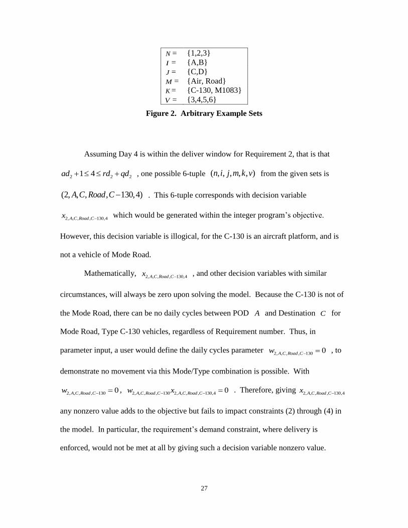
27

N = {1,2,3}

I = {A,B}

J = {C,D}

M = {Air, Road}

K = {C-130, M1083}

V = {3,4,5,6}

Figure 2. Arbitrary Example Sets

Assuming Day 4 is within the deliver window for Requirement 2, that is that

2 2 21 4ad rd qd , one possible 6-tuple ( , , , , , )n i j m k v from the given sets is

(2, , , , 130,4)A C Road C . This 6-tuple corresponds with decision variable

2, , , , 130,4A C Road Cx which would be generated within the integer program’s objective.

However, this decision variable is illogical, for the C-130 is an aircraft platform, and is

not a vehicle of Mode Road.

Mathematically, 2, , , , 130,4A C Road Cx

, and other decision variables with similar

circumstances, will always be zero upon solving the model. Because the C-130 is not of

the Mode Road, there can be no daily cycles between POD A and Destination C for

Mode Road, Type C-130 vehicles, regardless of Requirement number. Thus, in

parameter input, a user would define the daily cycles parameter 2, , , , 130 0A C Road Cw , to

demonstrate no movement via this Mode/Type combination is possible. With

2, , , , 130 0A C Road Cw , 2, , , , 130 2, , , , 130,4 0A C Road C A C Road Cw x . Therefore, giving

2, , , , 130,4A C Road Cx

any nonzero value adds to the objective but fails to impact constraints (2) through (4) in

the model. In particular, the requirement’s demand constraint, where delivery is

enforced, would not be met at all by giving such a decision variable nonzero value.

28

Therefore, the TDM does not give variables such as 2, , , , 130,4A C Road Cx

a nonzero value as

that would absolutely increase the objective while failing to impact any of the constraints.

Thus, because this decision variable, and others like it, will always be zero and have no

impact on the solution, they should not be generated and included in the model. The

same can be said for extraneous decision variables unnecessarily generated by TDM

constraints.

In addition to extraneous variables being generated by the model, the TDM also

creates numerous unnecessary constraints with a right-hand side (RHS) of 0. For

example, recall our sample sets in Figure 2. Again, assume that Requirement 2 is to be

delivered from A to C and has weight of 100 short tons. Then 2, , 100A Cr , by

definition of parameter nijr . Furthermore,

2, , 2, , 2, , 0A D B C B Dr r r because

Requirement 2 is not delivered along any of those POD i , Destination j pairs. Then

when implementing Constraints (2) for all combinations of i and j with 2n , the

following four constraints are obtained:

1

100 2, ,n n

n

rd q

nijmk k nijmkv

M K v ad

w p x n i A j C

1

0 2, ,n n

n

rd q

nijmk k nijmkv

M K v ad

w p x n i A j D

1

0 2, ,n n

n

rd q

nijmk k nijmkv

M K v ad

w p x n i B j C

1

0 2, ,n n

n

rd q

nijmk k nijmkv

M K v ad

w p x n i B j D

29

Note that the latter three constraints are completely unnecessary. As the TDM

assumes that each of , , 0nijmkv nijmk kx w p , it is clear that the latter three constraints

above will always be trivially greater than or equal to 0 and thus satisfied. Therefore,

their inclusion in the model is unwarranted because the constraints will always be

satisfied regardless of decision variable or parameter values. A similar happening occurs

with the TDM’s outloading and unloading constraints in that extra unneeded constraints

may also be created.

While including superfluous decision variables with a value of zero and

unnecessary constraints in the model will not dictate different solutions, it may have

drastic impacts on memory allocation and problem size. Recall that a large scale TPFDD

may have thousands of requirements, hundreds of Days, and numerous PODs,

Destinations, Modes, and Vehicles. Thus, as the problem increases in size, many more

6-tuples ( , , , , , )n i j m k v are possible and thus many more decision variables must be

generated even though many may, by default, have value of 0 as discussed above. This

causes the constraint matrix to become increasingly sparse, possibly causing problems to

become intractable if enough computer memory is not available to generate or solve the

problem. Even if the problem is tractable, the extraneous variables and unnecessary

constraints increase the problem size and thus slow solution time.

To avoid this dilemma, a Reduced Theater Distribution Model (RTDM) is

designed which sensibly reduces the problem while keeping all necessary variables and

constraints intact. This is done in two ways. Firstly, decision variables are generated by

the model only when there exists a chance for a decision variable to become nonzero,

which implies that a vehicle allocation is theoretically possible. Secondly, constraints

30

that do not affect the feasible space are not entered into the model. These problem

reducing concepts are implemented with a series of decomposing sets and binary

functions which are used to determine which portions of a set to sum through, as well as

which constraints are valid and necessary constraints to include in the model.

RTDM Overview.

While the parameters and decision variables from the TDM remained unchanged

in the RTDM, new sets are introduced with the purpose of reducing model sparsity and

ridding the problem of unnecessary variables and constraints. This assists in quicker

model generation. Some of the sets are simple decomposing sets and some sets require

the use of binary functions to determine inclusion. These sets, paired with an adjusted

formulation, greatly reduce the problem size while keeping the concepts and intent of the

TDM fully intact. This subsection will detail changes to the sets that are utilized in the

RTDM.

Firstly, new decomposing sets are introduced. These sets simply decompose the

original TDM sets of ,M K and N . The set ijM is introduced to describe the eligible

modes that may be selected between any POD i and Destination j . For example, if

Air and Road are possible transportation modes between i and j , but Rail is not, then

{ , , }M Air Road Rail yet { , }ijM Air Road . The RTDM also introduces the set mK

which describes the set of vehicles Types k K which are of Mode m . For example,

AirK may contain the air platforms C-130, C-5, and C-17. The set iN is introduced to

include only requirements n N such that Requirement n departs POD i . Likewise,

the set jN is introduced to include only requirements n N such that Requirement n

31

arrives at Destination j . These decomposing sets are easily determined with

preprocessing and are of great value in reducing problem size by eliminating extraneous

decision variable creation within constraints.

In addition to the decomposing sets, the RTDM also utilizes five Function

Derived Tuple Sets: VOTM , VLM , VR , VO , and VU . Binary functions are

used to evaluate the inclusion of tuples within these sets. Thus, these sets can be utilized

to determine which tuples’ corresponding variables should be included within the

objective and constraints. Functions (6) to (11) below describe the binary functions used

to create the new sets.

1, if Requirement delivered on Day would be on-time ( , )

0, otherwise

n vA n v

(6)

1, if Requirement delivered on Day would be late ( , )

0, otherwise

n vB n v

(7)

1, if vehicle of Type is also a Mode vehicle( , )

0, otherwise

k mC m k

(8)

1, if Requirement is to be delivered from POD to Destination ( , , )

0, otherwise

n i jD n i j

(9)

1, if some Requirement that may outload at POD onto a Mode vehicle on day ( , , )

0, otherwise

n i m vE i m v

(10)

1, if some Requirement that may unload at Destination off of a Mode vehicle on day ( , , )

0, otherwise

n j m vF j m v

(11)

32

The first set, VOTM , describes 6-tuples which are utilized in the decision

variables nijmkvx . The set VOTM , or Valid On Time Movements, yields tuples which

correspond to decision variables indicating valid, on-time movements. Mathematically,

{( , , , , , ) | ( , ) ( , ) ( , , ) 1}VOTM n i j m k v A n v C m k D n i j . This implies that Requirement

n is eligible to deliver from POD i to Destination j via a Mode m , Type k

vehicle on Day v where nv rd . Proper decision variable tuples in VOTM may not

have Mode/Type mismatches, delivery Days after the RDD, or POD/Destination pairs

that are not the proper, designated POD and Destination for specific requirements. Thus,

for decision variables nijmkvx , Functions (6), (8), and (9) work together to determine if

the corresponding 6-tuple ( , , , , , )n i j m k v warrants inclusion in the set VOTM .

Function (6) determines if Requirement n would be on-time if shipped on Day v .

Function (8) determines if a Type k vehicle is of Mode m and Function (9) checks to

ensure that Requirement n ships from i to j . Only if all functions return a value of

1, and thus the product of the functions is also 1, will the 6-tuple be included in the set

VOTM and the corresponding decision variable be generated and placed in the

objective.

The second set, VLM , also describes 6-tuples which are utilized in the decision

variables. The set VLM corresponds to decision variables for Requirement n

shipping from POD i to Destination j via a Mode m , Type k vehicle on Day v

such that n n nrd v rd qd . This set is dissimilar to VOTM in that it describes

6-tuples ( , , , , , )n i j m k v whose corresponding decision variable would indicate a

33

requirement being delivered past the RDD. Inclusion in VLM requires that a 6-tuple’s

associated decision variable not imply a Mode/Type mismatch, POD/Destination

mismatch, or delivery prior to or on the RDD. Therefore,

{( , , , , , ) | ( , ) ( , ) ( , , ) 1}VLM n i j m k v B n v C m k D n i j . Functions (8), and (9) work as

described in VOTM and Function (7) determines if the decision variable would indicate

Requirement n being delivered late after the RDD. If such conditions are met, a

6-tuple’s corresponding decision variable will be generated and included in the objective

function.

The final three Function Derived Tuple Sets are utilized for ridding the

formulation of unnecessary constraints. The set of Valid Routes is defined by Function

(9). That is, {( , , ) | ( , , ) 1}VR n i j D n i j . As each Requirement n has only a single

POD i and Destination j , there is only a single 3-tuple for each Requirement n that

describes its one and only Valid Route. Function (10) checks whether or not for a given

3-tuple ( , , )i m v , some Requirement n N may outload at POD i onto a Mode m

vehicle on Day v . This is used to construct the set of Valid Outload tuples, VO .

Mathematically, {( , , ) | ( , , ) 1}VO i m v E i m v . Likewise, Function (11) utilizes the

same methodology to construct Valid Unload tuples, VU . The set VU is defined

mathematically by {( , , ) | ( , , ) 1}VU j m v F j m v . All of the new sets discussed lead

to the reduced formulation of the RTDM by eliminating extraneous decision variables

and unnecessary constraints from the problem. Table 5 - Table 8 below summarize the

sets, parameters, and decision variables utilized in the pure integer programming RTDM.

34

Table 5. RTDM Basic Sets

Set Description


I Set of all PODs i





ijM Set of all Modes m with direct paths between POD i and Destination j

mK Set of all vehicle Types k which are of Mode m

iN Set of movement Requirements n that depart from POD i

jN Set of movement Requirements n that arrive at Destination j

Table 6. RTDM Function Derived Tuple Sets

Set Description Mathematical Notation

VOTM Valid On-Time

Movements

{( , , , , , ) | ( , ) ( , ) ( , , ) 1}n i j m k v A n v C m k D n i j

VLM Valid Late Movements {( , , , , , ) | ( , ) ( , ) ( , , ) 1}n i j m k v B n v C m k D n i j

VR Valid Routes {( , , ) | ( , , ) 1} n i j D n i j

VO Valid Outloading {( , , ) | ( , , ) 1}i m v E i m v

VU Valid Unloading {( , , ) | ( , , ) 1}j m v F j m v

35

Table 7. RTDM Parameters









nqd Maximum allowable extention days beyond RDD in which

Requirement n can be delivered to given destination (with penalty) g Late penalty per vehicle per day


i on Day v



nijmkw Number of possible cycles in a day between POD i and Destination

j via Mode m , Type k vehicles transporting Requirement n

Table 8. RTDM Decision Variables

Variables Description

nijmkvx Number of vehicles of Mode m , Type k that are required on Day v

to deliver Requirement n from POD i to Destination j

RTDM Formulation.

The RTDM, which greatly reduces problem size, is shown below in Model 2.

36

( , , , , , ) ( , , , , , )

Minimize ( )k nijmkv n nijmkv

n i j m k v VOTM VLM n i j m k v VLM

b x g v rd x

(12)

Subject to

1

( , , )n n

ij m n

rd q

nijmk k nijmkv nij

M K v ad

w p x r n i j VR

(13)

( , , )i m

nijmk nijmkv imv

N J K

w x o i m v VO (14)

( , , )j m

nijmk nijmkv jmv

N I K

w x u j m v VU (15)

{0} ( , , , , , )nijmkvx n i j m k v VOTM VLM (16)

Model 2. Reduced Theater Distribution Model (RTDM)

The purpose of the RTDM objective and constraints remain the same as discussed

in the original TDM (page 20)—to find on-time, least-cost vehicle allocations to

accomplish delivery. However, the model is reduced significantly by taking advantage of

the new sets introduced in the RTDM Overview subsection. With the RTDM, the

objective (12) retains the purpose of minimizing both vehicle utilization costs and

penalties for utilizing vehicles for late deliveries.

By summing across all 6-tuples in VOTM VLM , the first part of the objective

function multiplies vehicle operating cost kb and decision variable nijmkvx for each and

every theoretically possible decision variable. However, no extraneous decision

37

variables, those with 6-tuples ( , , , , , )n i j m k v VOTM VLM , are generated. Likewise,

only the logical decision variables whose 6-tuples correspond to late movements, that is

those where ( , , , , , )n i j m k v VLM , are multiplied by the penalty factor. Thus, the

objective function includes the all theoretically possible decision variables and associated

costs and penalties.

The RTDM constraints shown in (13) to (16) are the demand, outloading,

unloading, and integrality constraints for the model. These are similar to (2) through (5)

of the TDM. However, the left-hand side (LHS) summations in the RTDM constraints do

not simply go across entire sets. Instead, some decomposing sets are utilized, which

keeps extraneous variables from being created. Additionally, the “for all” statements for

each general constraint that dictate which combinations of variables are used to generate

a constraint are restricted in the RTDM. Recall that the TDM generated constraints for

each and every combination of indices for the requirement, outloading, and unloading

constraints. However, this is not necessary and thus the RTDM ensures a totally reduced

format.

In the demand constraint at (13), the LHS summation is across sets ijM , mK ,

and appropriate values of v . Thus, the decomposed sets ensure extraneous variables

are not included in the model. Likewise, only necessary demand constraints are included

in the model because a constraint is only generated for ( , , )n i j VR . Thus, the use of

the Function Derived Tuple Set VR ensures that unnecessary constraints are not

generated when the 3-tuple ( , , )n i j is illogical.

38

In the outload and unload constraints at (14) and (15), the sets iN and jN ,

respectively, are utilized in the LHS summations in place of the set N as was done in

the TDM. Additionally, the set mK is utilized rather than K . Again, the use of these

decomposing sets ensures that extraneous variables are not generated in the RTDM.

Furthermore, 3-tuples are checked for inclusion in the Function Derived Tuple Sets to

check if a constraint should be made. A 3-tuple in VO will generate a necessary outload

constraint and a 3-tuple in VU will generate an unloading constraint. Constraints are

not constructed for 3-tuples not included in VO or VU as they would have no impact

on the feasible space.

RTDM Conclusion.

By restricting the objective function to consider only theoretically possible

variables, and using decomposing sets on summations on the LHS of the constraints, the

RTDM ensures that no extraneous decision variables are created. Only those decision

variables that may theoretically take on nonzero value are included. Properly conducted

preprocessing and the use of binary functions to determine set inclusion guarantees that

no decision variable is taken out that could potentially take on a nonzero value.

Furthermore, limiting the tuples for which constraints are generated reduces the total

number of constraints in the model. Because only extraneous decision variables are

removed and no constraints that affect the feasible space are removed, solving the same

arbitrary problem with both the TDM and RTDM should yield the same objective value

and solution. The difference will be in number of decision variables, number of

constraints, and problem size. Thus, a reduced formulation yielding the same vehicle

39

allocations given by the TDM can be successfully, and more easily, generated and

attained with the RTDM.

Improved Theater Distribution Model (ITDM)

ITDM Motivation.

While the RTDM greatly reduces problem size by removing extraneous decision

variables and unnecessary constraints, the core of the modeling formulation remains

unchanged from the TDM. The RTDM’s pure integer programming formulation includes

an objective for on-time least cost vehicle mixtures along with three general constraints

which are demand, outloading, and unloading. However, research into RTDM solutions

indicate changes are needed to the formulation, particularly with respect to new decision

variables and constraints. Thus, a mixed integer linear program is developed, known as

the Improved Theater Distribution Model (ITDM) which improves upon the pure integer

program RTDM. In making these new additions, the ITDM also requires some new sets

to make certain that, like the RTDM, the ITDM is minimally formulated to ensure no

extraneous decision variables or unnecessary constraints are generated. The ITDM is the

main contribution of this research, encompassing both model reduction and a new mixed

integer programming approach to force flow analysis.

Recall that the decision variable of the TDM and RTDM was nijmkvx ,

representing the number of vehicles of Mode m , Type k that are required on Day v

to deliver Requirement n from POD i to Destination j . That is, each requirement

is associated with a specific mixture of vehicles and accompanying delivery dates,

indicated by those decision variables assuming nonzero value. However, there is an

inherent flaw in this choice of decision variable as it requires that each Requirement n

40

be allocated at least one vehicle specifically for that requirement. This construct does not

necessary match reality. For example, consider two requirements, each with the exact

same attributes of POD, Destination, Arrival Date at POD nad and Required Delivery

Date at Destination nrd . If both requirements each weigh only 10 short tons, it

should be clear that the two requirements could possibly be allocated to a single 20 short

ton transport vehicle. However, modeling with the RTDM (or TDM) would not allow

this, as each vehicle is specifically matched with a requirement due to decision variables

having an index of Requirement n . The mixed integer formulation presented in the

ITDM overcomes this shortfall.

The RTDM also models lateness poorly and the ITDM addresses this. This

improvement is important as a model that inappropriately models lateness may give

solutions that are not truly representative of the best on-time, least-cost solution. Recall

that in the TDM/RTDM formulations, lateness was penalized per vehicle per day late.

However, it is clear that two vehicles arriving equally late would not necessarily deserve

to be penalized equally. Arbitrarily, assume that a truck delivers only two short tons late

while an aircraft delivers 50 short tons late. Logically, the aircraft holding the larger

cargo shipment should be penalized more severely for lateness. However, the RTDM

does not consider this. The RTDM only measures the truck and the aircraft as a single,

late vehicle. However, the ITDM penalizes lateness not by measuring the number of

vehicles that arrive late per day, but rather, how many short tons arrive late per day. The

next subsection will explain concepts developed in the ITDM before the model

formulation is given.

41

ITDM Overview.

The ITDM has two different types of decision variables. Rather than examining

vehicle decisions only as with the RTDM, the ITDM has one set of decision variables to

model the flow of requirement short tonnage throughout the network and another to

represent the vehicles necessary to support these flows. Continuous decision variables

nijmkvy are utilized to represent the number of short tons of Requirement n being

delivered by a Mode m , Type k vehicle from POD i to Destination j on Day v .

Additionally, the integer decision variable ijmkvx is used, representing the number of

vehicles of Mode m , Type k that are needed on Day v to deliver any requirements

from POD i to Destination j . Note that the integer vehicle variables are not tied to

any particular requirement number, n . Thus, the vehicle allocations dictated by

decision variables ijmkvx may embody the movement of one, or many different

requirements. Furthermore, both on-time and late cargo may be delivered on the same

vehicle. The use of both continuous and integer decision variables allows for a much

more accurate representation vehicle use.

In regards to sets utilized in the ITDM, many are carried over from the RTDM

(page 34), namely the sets , , , , , , , , , ,m ijN I J M K V K M VR VO and VU . Like the

RTDM, the ITDM addresses model reduction. However, the ITDM’s differing decision

variables causes some different decomposing sets and Function Derived Tuple Sets to be

implemented in the ITDM. The RTDM sets ,, iVOTM N and

jN are not utilized in the

ITDM. Four new sets are introduced with the ITDM, three of which are derived from

functions as well as a single new decomposing set. Together, these new sets work to

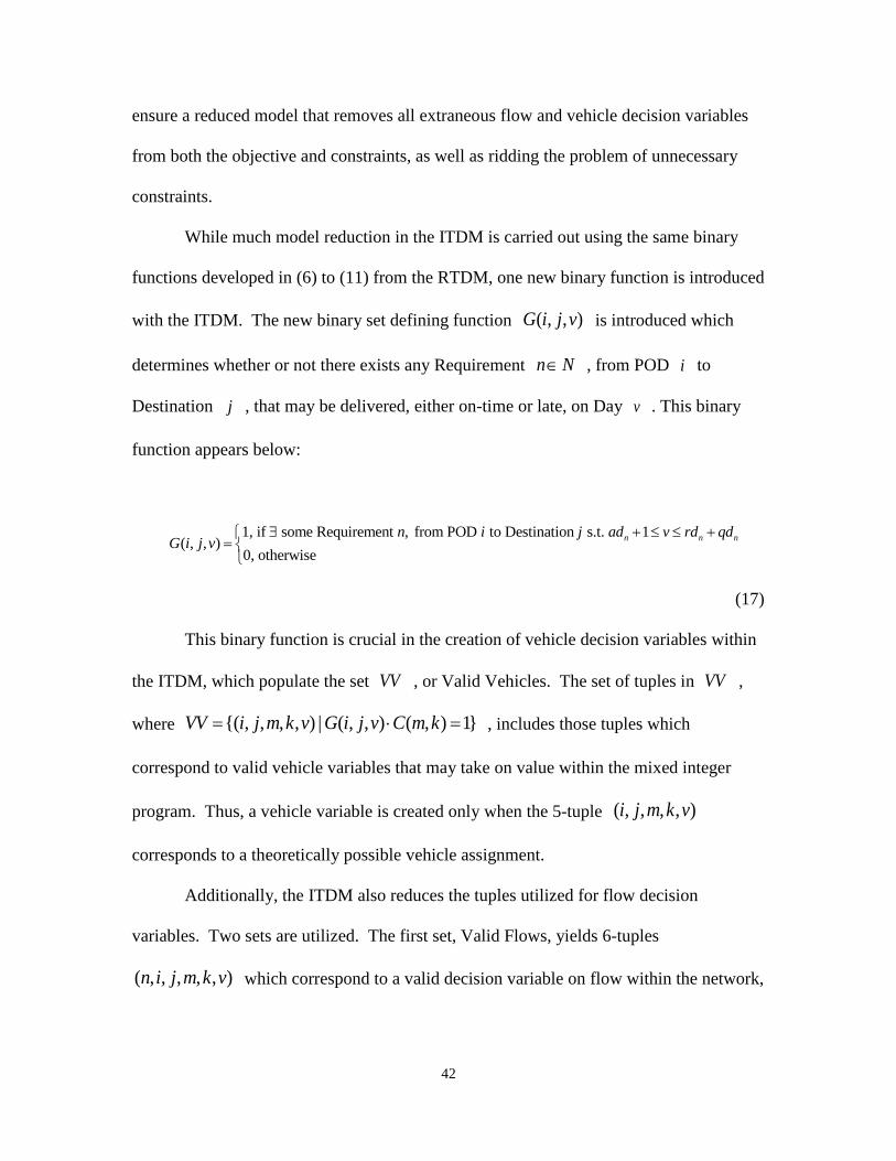
42

ensure a reduced model that removes all extraneous flow and vehicle decision variables

from both the objective and constraints, as well as ridding the problem of unnecessary

constraints.

While much model reduction in the ITDM is carried out using the same binary

functions developed in (6) to (11) from the RTDM, one new binary function is introduced

with the ITDM. The new binary set defining function ( , , )G i j v is introduced which

determines whether or not there exists any Requirement n N , from POD i to

Destination j , that may be delivered, either on-time or late, on Day v . This binary

function appears below:

1, if some Requirement , from POD to Destination s.t. 1

( , , )0, otherwise

n n nn i j ad v rd qdG i j v

(17)

This binary function is crucial in the creation of vehicle decision variables within

the ITDM, which populate the set VV , or Valid Vehicles. The set of tuples in VV ,

where {( , , , , ) | ( , , ) ( , ) 1}VV i j m k v G i j v C m k , includes those tuples which

correspond to valid vehicle variables that may take on value within the mixed integer

program. Thus, a vehicle variable is created only when the 5-tuple ( , , , , )i j m k v

corresponds to a theoretically possible vehicle assignment.

Additionally, the ITDM also reduces the tuples utilized for flow decision

variables. Two sets are utilized. The first set, Valid Flows, yields 6-tuples

( , , , , , )n i j m k v which correspond to a valid decision variable on flow within the network,

43

both on-time and late. This set is defined mathematically as

{( , , , , , ) | ( , ) ( , ) ( , , ) ( , ) ( , ) ( , , ) 1}VF n i j m k v A n v C m k D n i j B n v C m k D n i j .

Additionally, the set Late Flows describes valid 6-tuples which correspond to a valid flow

decision variable which indicate late movement. Mathematically, this set is defined as

{( , , , , , ) | ( , ) ( , ) ( , , ) 1}LF n i j m k v B n v C m k D n i j . Note that LF is mathematically

equivalent to the RTDM set VLM . However, the tuples in this case correspond to flow

variables, not vehicle variables.

The decomposing set ijvN is also introduced which includes all requirements

n N which are to be delivered from POD i to Destination j and are eligible to

deliver on Day v . This set is crucial to one of the main constraints of the problem, the

vehicle linking constraint, which ensures that enough vehicles are allocated to move the

necessary requirements.

The parameters of the ITDM remain mostly the same, save for two slight, yet

important, adjustments. Firstly, the penalty parameter, g , no longer represents the

penalty per vehicle per day late. This is because in the ITDM, lateness is measured by

short tons delivered late rather than vehicles delivering late. Thus, in the ITDM, the

penalty variable g actually represents the late penalty per short ton per day delivered

late. The cycle parameter also changes within the ITDM. While its purpose remains the

same, the index of n N is removed from the cycle parameter. Thus, in the ITDM,

cycles are given by the parameter ijmkw . Recall that in the TDM /RTDM formulations,

cycle values nijmkw were defined by their 5-tuples ( , , , , )n i j m k . However, because a

cycle is simply a time and distance calculation for a Mode m , Type k vehicle along

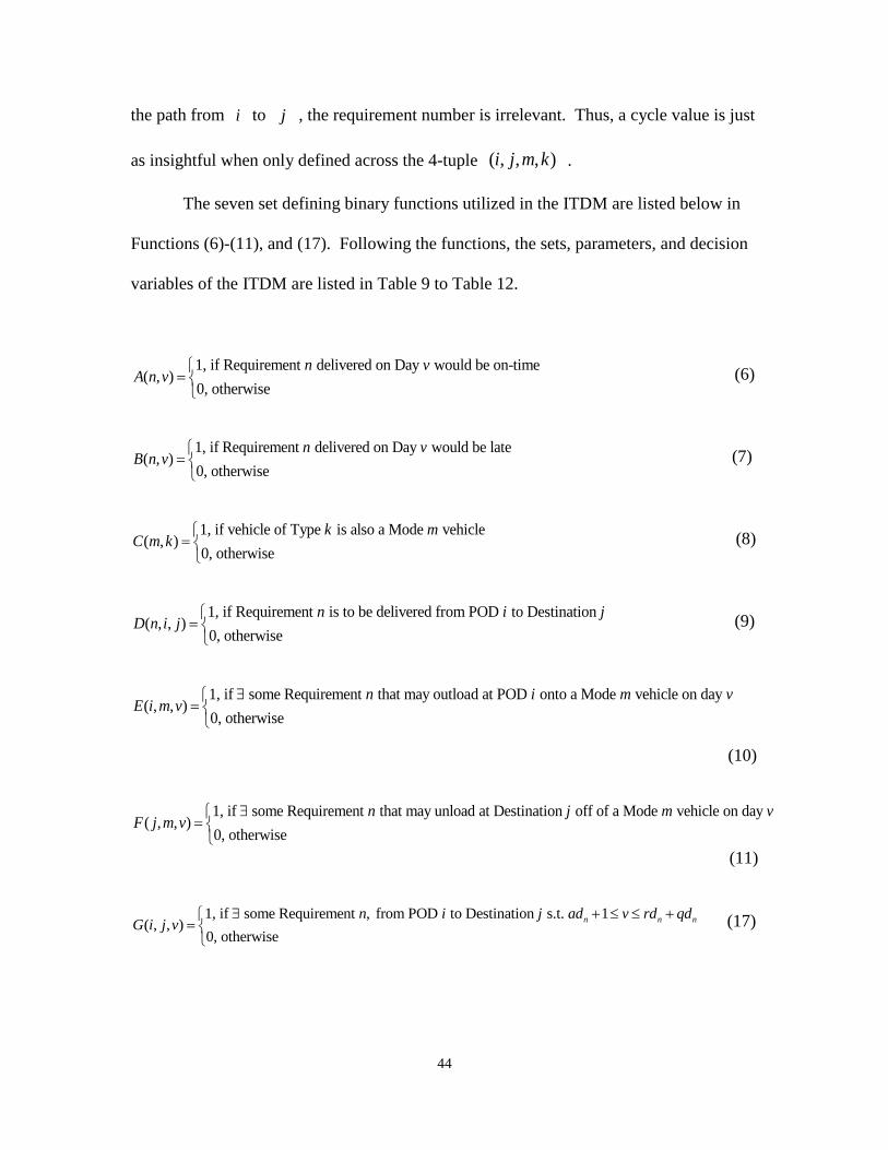
44

the path from i to j , the requirement number is irrelevant. Thus, a cycle value is just

as insightful when only defined across the 4-tuple ( , , , )i j m k .

The seven set defining binary functions utilized in the ITDM are listed below in

Functions (6)-(11), and (17). Following the functions, the sets, parameters, and decision

variables of the ITDM are listed in Table 9 to Table 12.

1, if Requirement delivered on Day would be on-time ( , )

0, otherwise

n vA n v

(6)

1, if Requirement delivered on Day would be late ( , )

0, otherwise

n vB n v

(7)

1, if vehicle of Type is also a Mode vehicle( , )

0, otherwise

k mC m k

(8)

1, if Requirement is to be delivered from POD to Destination ( , , )

0, otherwise

n i jD n i j

(9)

1, if some Requirement that may outload at POD onto a Mode vehicle on day ( , , )

0, otherwise

n i m vE i m v

(10)

1, if some Requirement that may unload at Destination off of a Mode vehicle on day ( , , )

0, otherwise

n j m vF j m v

(11)

1, if some Requirement , from POD to Destination s.t. 1( , , )

0, otherwise

n n nn i j ad v rd qdG i j v

(17)

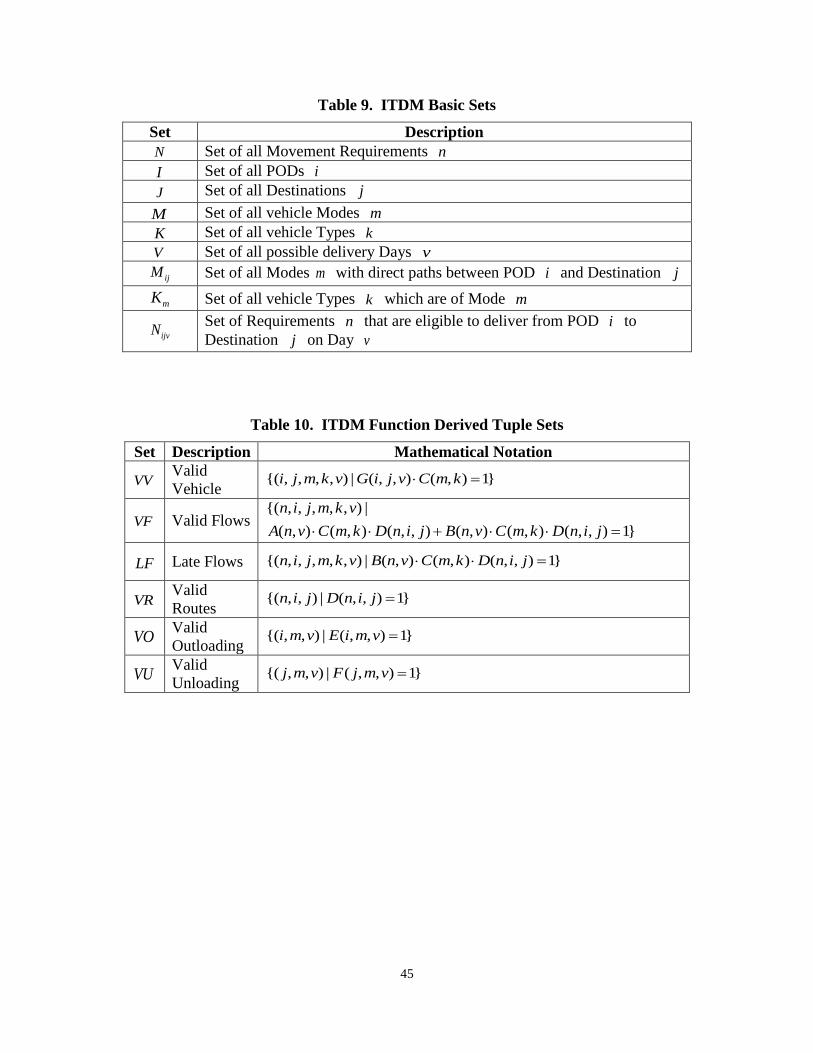
45

Table 9. ITDM Basic Sets

Set Description


I Set of all PODs i





ijM Set of all Modes m with direct paths between POD i and Destination j

mK Set of all vehicle Types k which are of Mode m

ijvN Set of Requirements n that are eligible to deliver from POD i to


Table 10. ITDM Function Derived Tuple Sets

Set Description Mathematical Notation

VV Valid

Vehicle {( , , , , ) | ( , , ) ( , ) 1} i j m k v G i j v C m k

VF Valid Flows {( , , , , , ) |

( , ) ( , ) ( , , ) ( , ) ( , ) ( , , ) 1}

n i j m k v

A n v C m k D n i j B n v C m k D n i j

LF Late Flows {( , , , , , ) | ( , ) ( , ) ( , , ) 1} n i j m k v B n v C m k D n i j

VR Valid

Routes {( , , ) | ( , , ) 1} n i j D n i j

VO Valid

Outloading {( , , ) | ( , , ) 1}i m v E i m v

VU Valid

Unloading {( , , ) | ( , , ) 1}j m v F j m v

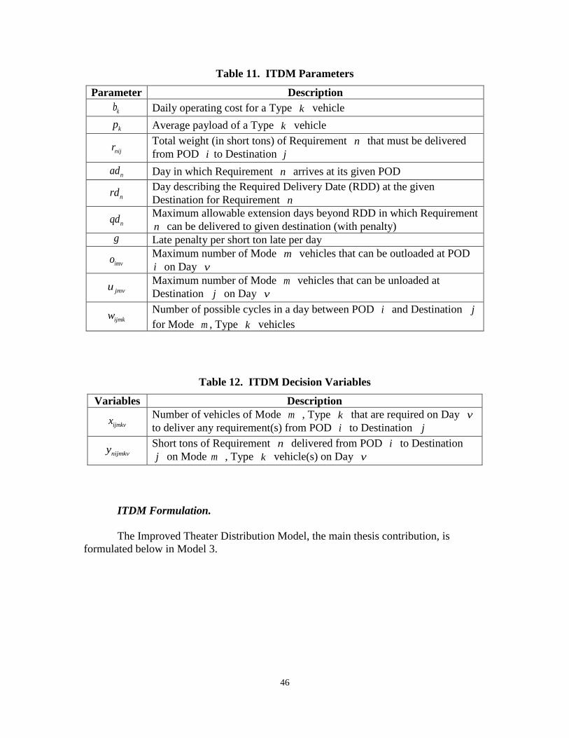
46

Table 11. ITDM Parameters









nqd Maximum allowable extension days beyond RDD in which Requirement

n can be delivered to given destination (with penalty) g Late penalty per short ton late per day


i on Day v



ijmkw Number of possible cycles in a day between POD i and Destination j

for Mode m , Type k vehicles

Table 12. ITDM Decision Variables

Variables Description

ijmkvx Number of vehicles of Mode m , Type k that are required on Day v

to deliver any requirement(s) from POD i to Destination j

nijmkvy Short tons of Requirement n delivered from POD i to Destination

j on Mode m , Type k vehicle(s) on Day v

ITDM Formulation.

The Improved Theater Distribution Model, the main thesis contribution, is

formulated below in Model 3.

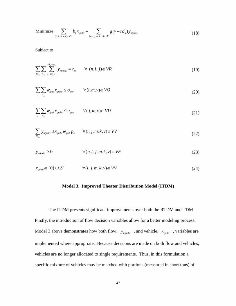
47

( , , , , ) ( , , , , , )

Minimize ( )k ijmkv n nijmkv

i j m k v VV n i j m k v LF

b x g v rd y

(18)

Subject to

1

( , , )n n

ij m n

rd q

nijmkv nij

M K v ad

y r n i j VR

(19)

( , , )m

ijmk ijmkv imv

J K

w x o i m v VO (20)

( , , )m

ijmk ijmkv jmv

I K

w x u j m v VU (21)

( , , , , )ijv

nijmkv ijmkv ijmk k

N

y x w p i j m k v VV (22)

0 ( , , , , , )nijmkvy n i j m k v VF (23)

{0} ( , , , , )ijmkvx i j m k v VV (24)

Model 3. Improved Theater Distribution Model (ITDM)

The ITDM presents significant improvements over both the RTDM and TDM.

Firstly, the introduction of flow decision variables allow for a better modeling process.

Model 3 above demonstrates how both flow, nijmkvy , and vehicle,

ijmkvx , variables are

implemented where appropriate. Because decisions are made on both flow and vehicles,

vehicles are no longer allocated to single requirements. Thus, in this formulation a

specific mixture of vehicles may be matched with portions (measured in short tons) of

48

requirements. Each vehicle mixture could support partial requirements or one or multiple

requirements together. Because vehicles are no longer tied to specific requirements, a

much more accurate modeling process is achieved.

The ITDM objective, given in (18), attempts to minimize vehicle costs while also

looking to minimize penalties associated with the short tons being delivered late. Thus,

optimal solutions to the ITDM will not necessarily include a minimal number of late

vehicles, but rather a minimal number of late short tons. This presents a more realistic

objective in terms of real-world considerations.

Constraints at (19) ensure that the sum of valid flow variables are large enough to

equal the demand associated with each requirement. That is, each requirement must have

associated flows that will meet the requirement’s weight. Constraints at (20) and (21)

ensure that the number of vehicles selected by the model do not exceed the outloading

and unloading capacities, respectively. The TDM and RTDM had similar constraints,

however, formulation is different because vehicles are no longer tied to specific

requirements. Thus, no information on the requirement number is needed within these

two outloading and unloading constraints as they are concerned only with vehicles.

The vehicle linking constraint at (22) is what ties together the continuous flow

variables and the integer vehicle variables. It ensures that, for flow decisions

corresponding to matching ( , , , , )i j m k v values, enough vehicles are allocated to provide

transportation capacity for appropriate requirements included as part of those flows. This

allows vehicles to hold cargo from a number of different requirements. The constraint

also allows late cargo from some number of requirements to be delivered with on-time

cargo from other requirements. In a real-world scenario, there is nothing that would

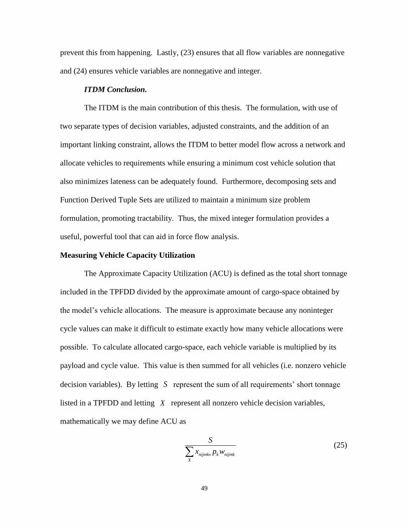
49

prevent this from happening. Lastly, (23) ensures that all flow variables are nonnegative

and (24) ensures vehicle variables are nonnegative and integer.

ITDM Conclusion.

The ITDM is the main contribution of this thesis. The formulation, with use of

two separate types of decision variables, adjusted constraints, and the addition of an

important linking constraint, allows the ITDM to better model flow across a network and

allocate vehicles to requirements while ensuring a minimum cost vehicle solution that

also minimizes lateness can be adequately found. Furthermore, decomposing sets and

Function Derived Tuple Sets are utilized to maintain a minimum size problem

formulation, promoting tractability. Thus, the mixed integer formulation provides a

useful, powerful tool that can aid in force flow analysis.

Measuring Vehicle Capacity Utilization

The Approximate Capacity Utilization (ACU) is defined as the total short tonnage

included in the TPFDD divided by the approximate amount of cargo-space obtained by

the model’s vehicle allocations. The measure is approximate because any noninteger

cycle values can make it difficult to estimate exactly how many vehicle allocations were

possible. To calculate allocated cargo-space, each vehicle variable is multiplied by its

payload and cycle value. This value is then summed for all vehicles (i.e. nonzero vehicle

decision variables). By letting S represent the sum of all requirements’ short tonnage

listed in a TPFDD and letting X represent all nonzero vehicle decision variables,

mathematically we may define ACU as

nijmkv k nijmk

X

S

x p w (25)

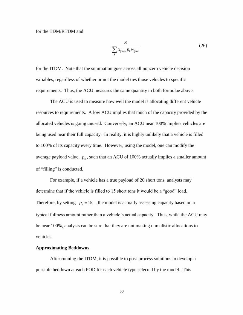
50

for the TDM/RTDM and

ijmkv k ijmk

X

S

x p w (26)

for the ITDM. Note that the summation goes across all nonzero vehicle decision

variables, regardless of whether or not the model ties those vehicles to specific

requirements. Thus, the ACU measures the same quantity in both formulae above.

The ACU is used to measure how well the model is allocating different vehicle

resources to requirements. A low ACU implies that much of the capacity provided by the

allocated vehicles is going unused. Conversely, an ACU near 100% implies vehicles are

being used near their full capacity. In reality, it is highly unlikely that a vehicle is filled

to 100% of its capacity every time. However, using the model, one can modify the

average payload value, kp , such that an ACU of 100% actually implies a smaller amount

of “filling” is conducted.

For example, if a vehicle has a true payload of 20 short tons, analysts may

determine that if the vehicle is filled to 15 short tons it would be a “good” load.

Therefore, by setting 15kp , the model is actually assessing capacity based on a

typical fullness amount rather than a vehicle’s actual capacity. Thus, while the ACU may

be near 100%, analysts can be sure that they are not making unrealistic allocations to

vehicles.

Approximating Beddowns

After running the ITDM, it is possible to post-process solutions to develop a

possible beddown at each POD for each vehicle type selected by the model. This

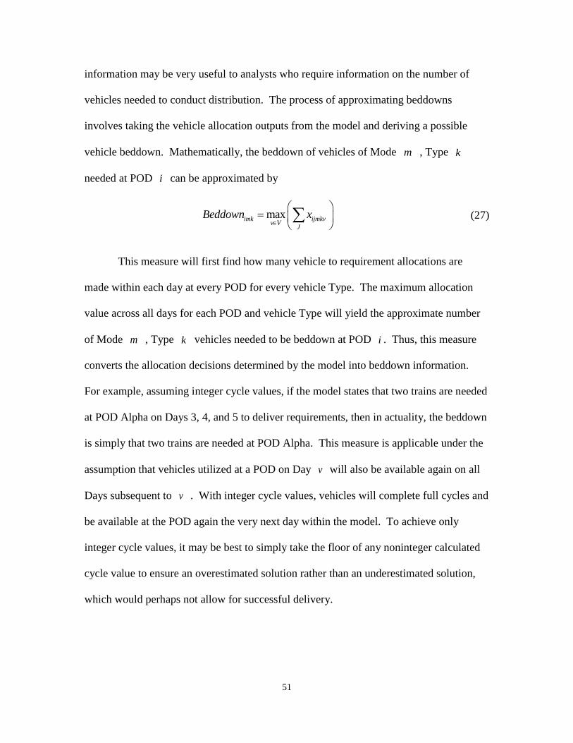
51

information may be very useful to analysts who require information on the number of

vehicles needed to conduct distribution. The process of approximating beddowns

involves taking the vehicle allocation outputs from the model and deriving a possible

vehicle beddown. Mathematically, the beddown of vehicles of Mode m , Type k

needed at POD i can be approximated by

maximk ijmkvv V

J

Beddown x

(27)

This measure will first find how many vehicle to requirement allocations are

made within each day at every POD for every vehicle Type. The maximum allocation

value across all days for each POD and vehicle Type will yield the approximate number

of Mode m , Type k vehicles needed to be beddown at POD i . Thus, this measure

converts the allocation decisions determined by the model into beddown information.

For example, assuming integer cycle values, if the model states that two trains are needed

at POD Alpha on Days 3, 4, and 5 to deliver requirements, then in actuality, the beddown

is simply that two trains are needed at POD Alpha. This measure is applicable under the

assumption that vehicles utilized at a POD on Day v will also be available again on all

Days subsequent to v . With integer cycle values, vehicles will complete full cycles and

be available at the POD again the very next day within the model. To achieve only

integer cycle values, it may be best to simply take the floor of any noninteger calculated

cycle value to ensure an overestimated solution rather than an underestimated solution,

which would perhaps not allow for successful delivery.

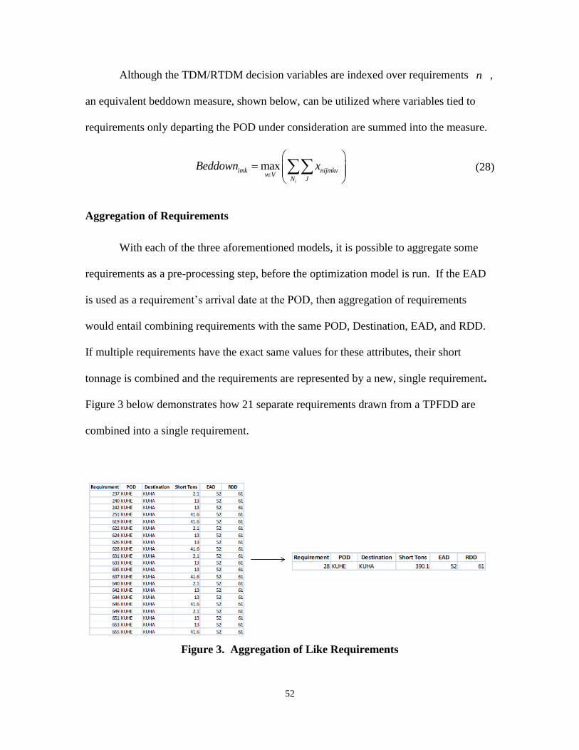
52

Although the TDM/RTDM decision variables are indexed over requirements n ,

an equivalent beddown measure, shown below, can be utilized where variables tied to

requirements only departing the POD under consideration are summed into the measure.

maxi

imk nijmkvv V

N J

Beddown x

(28)

Aggregation of Requirements

With each of the three aforementioned models, it is possible to aggregate some

requirements as a pre-processing step, before the optimization model is run. If the EAD

is used as a requirement’s arrival date at the POD, then aggregation of requirements

would entail combining requirements with the same POD, Destination, EAD, and RDD.

If multiple requirements have the exact same values for these attributes, their short

tonnage is combined and the requirements are represented by a new, single requirement.

Figure 3 below demonstrates how 21 separate requirements drawn from a TPFDD are

combined into a single requirement.

Figure 3. Aggregation of Like Requirements

53

Attaining fewer requirements will lead to fewer decision variables and may

impact the number of vehicles necessary for delivery. However, because extension days

are not listed on a TPFDD, but rather determined by commanders, aggregation may lead

to incorrectly assigned extension days. Furthermore, it is not possible to disaggregate

once aggregation has been conducted. Because aggregation may be implemented as a

pre-processing step in the TDM, RTDM, or ITDM, aggregation only affects the input,

specifically of requirements, into the model. The formulation and mathematics of each

model remain unchanged.

Conclusion

This chapter has extensively detailed the models developed in this research,

namely the RTDM and ITDM. The concept of aggregating requirements as a

preprocessing step for inputs was also discussed. Additionally, an approximating

measure for vehicle beddowns is introduced. The next chapter of this thesis will detail

the implementation of these models on a handful of different test cases.

54

IV. Implementation and Results

Implementation

The RTDM and ITDM presented in Chapter III, along with the TDM, were

implemented using both Microsoft Office Excel 2007 and the optimization software

LINGO 13 (Lindo Systems Inc, 2012). A Decision Support System was built in the

Excel environment where the user uploads a TPFDD and enters all other input parameters

for the model. Once all data has been entered, Visual Basic for Applications (VBA) code

is used within Excel to construct and write the math programming models to LINGO

files. Once built, these files are solved in LINGO 13. Upon completion, the raw solution

data is converted into information and then reported back within the Excel environment.

All testing was conducted on a Dell Precision T7500 computer running Windows Vista

(Service Pack 2) with two Intel Xeon W5590 processors and 48 GB of RAM.

To encourage fast solutions for larger models, a relative optimality tolerance

setting was utilized. The solver was set to search for the true optimal solution for the first

two minutes of solving. If, after those two minutes, the true optimal solution was not

found, feasible solutions found within at least 0.2% of the Linear Program Relaxation

lower bound were reported as globally optimal. Other LINGO 13 settings used in this

analysis are available in Appendix A.

Recall from Chapter III that the TDM and RTDM unnecessarily index cycle

parameters across requirement number n , as requirement numbers have no impact on

the cycle value itself. Because the ITDM addresses this, ITDM cycle inputs are not

indexed over the requirement number. Thus, two different cycle inputs are used in

55

testing depending upon the model being implemented. However, cycle parameters for

the ITDM were matched to align with the cycle parameters used in the TDM and RTDM.

Therefore, comparisons between models remain sound.

Model Testing

In this analysis, each model (TDM, RTDM, ITDM) was tested on three different

test cases. The first two test cases were entirely notional, while the third test case was a

large-scale problem with data typical of an actual TPFDD. In all cases, solutions were

found in less than 3 minutes, and small test cases (i.e. Test Cases 1 and 2) solved in less

than a second.

For each test case, solution information regarding the number of air, road, and rail

vehicle allocations made to requirements was collected. This information is drawn

directly from the nonzero vehicle decision variables. For example,

, , , 130,4 3KUHE KUHA Air Cx , implying that 3 C-130s are needed on day 4 to deliver

requirements from KUHE to KUHA, means that three vehicle allocations are made. Note

that if the cycle value with matching tuple to this decision variable is greater than 1, more

than one pickup and delivery is conducted with this allocation. For example, if

, , , 130 2KUHE KUHA Air Cw , then the three vehicle allocations actually imply six pickup and

deliveries were made. Approximate Capacity Utilization values were also collected

during testing.

Problem size information such as number of variables (integer and continuous)

and number of constraints were also recorded. Potential vehicle beddowns derived from

vehicle allocations are developed for the large scale solutions found in Test Case 3.

Also, an example of how different inputs can be utilized to model policy decisions is

56

shown using the ITDM. Lastly, model solutions are compared when the aggregation of

like requirements is conducted before optimization.

In all tests, it was assumed that requirements arrived at the POD on the EAD

stated in the TPFDD. Thus, for each requirement, nad is set to the requirement’s EAD.

Additionally, every requirement was given a single extension day within all test cases.

That is, 1nqd for all requirements.

Test Case 1.

The first test case utilized the exact TPFDD and data used as an example in the

internal research paper by Longhorn & Kovich (2012). The TPFDD for this case listed

16 movement requirements, two PODs, and two Destinations. The TPFDD is shown

below in Table 13. Note that the Short Tons column gives the nijr values, the EAD

column gives the nad values, and the RDD column gives the nrd values. Note also

that the possible delivery Days, including extension days, (i.e. the set V ) ranged

between Day 3 and Day 10. Three modes (Air, Rail, Road) and three vehicle Types

(C-130, M1083, and DODX) were utilized. The penalty per day per late vehicle

(TDM/RTDM) and penalty per day per short ton (ITDM) was set to 1,000,000g .

The payload, cost, outloading , unloading, and cycle parameters used are shown in

Appendix B.

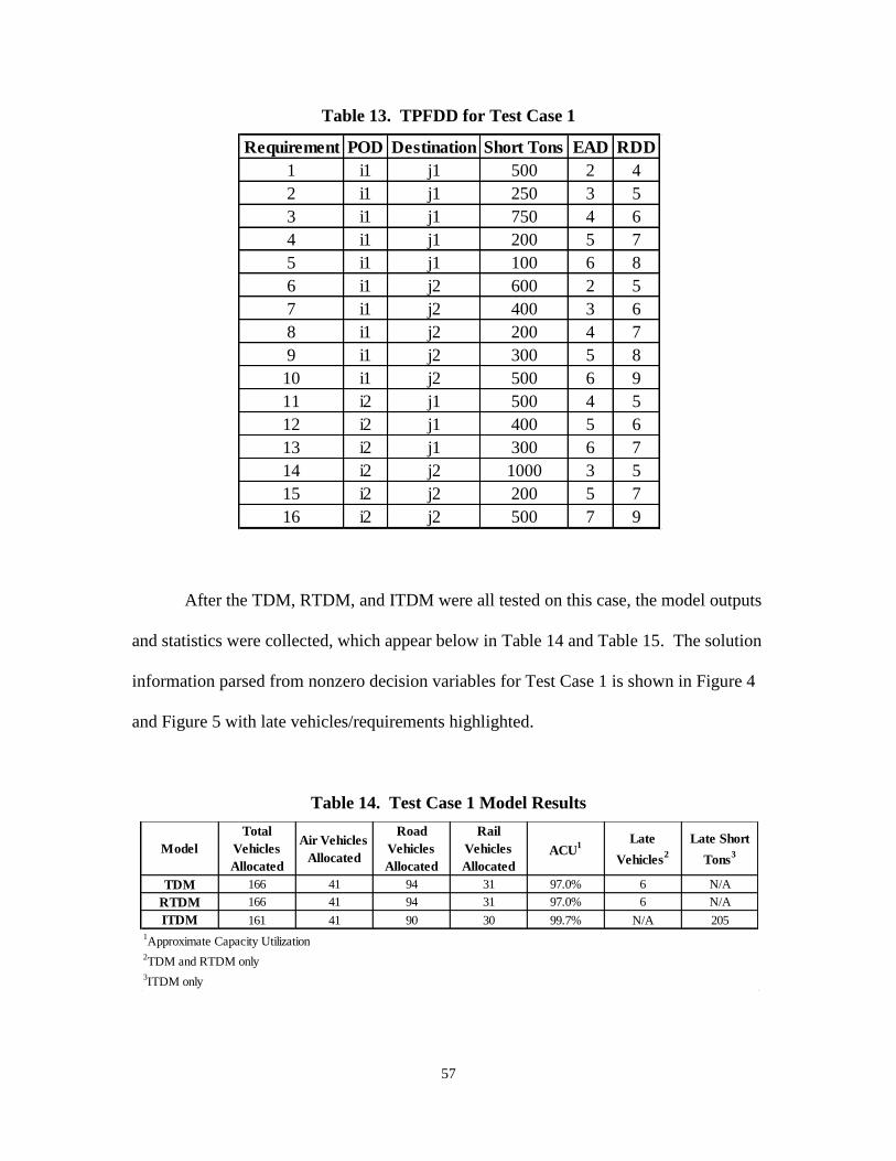
57

Table 13. TPFDD for Test Case 1

After the TDM, RTDM, and ITDM were all tested on this case, the model outputs

and statistics were collected, which appear below in Table 14 and Table 15. The solution

information parsed from nonzero decision variables for Test Case 1 is shown in Figure 4

and Figure 5 with late vehicles/requirements highlighted.

Table 14. Test Case 1 Model Results

Requirement POD Destination Short Tons EAD RDD

1 i1 j1 500 2 4

2 i1 j1 250 3 5

3 i1 j1 750 4 6

4 i1 j1 200 5 7

5 i1 j1 100 6 8

6 i1 j2 600 2 5

7 i1 j2 400 3 6

8 i1 j2 200 4 7

9 i1 j2 300 5 8

10 i1 j2 500 6 9

11 i2 j1 500 4 5

12 i2 j1 400 5 6

13 i2 j1 300 6 7

14 i2 j2 1000 3 5

15 i2 j2 200 5 7

16 i2 j2 500 7 9

Model

Total

Vehicles

Allocated

Air Vehicles

Allocated

Road

Vehicles

Allocated

Rail

Vehicles

Allocated

ACU1

Late

Vehicles2

Late Short

Tons3

TDM 166 41 94 31 97.0% 6 N/A

RTDM 166 41 94 31 97.0% 6 N/A

ITDM 161 41 90 30 99.7% N/A 205

1Approximate Capacity Utilization

2TDM and RTDM only

3ITDM only

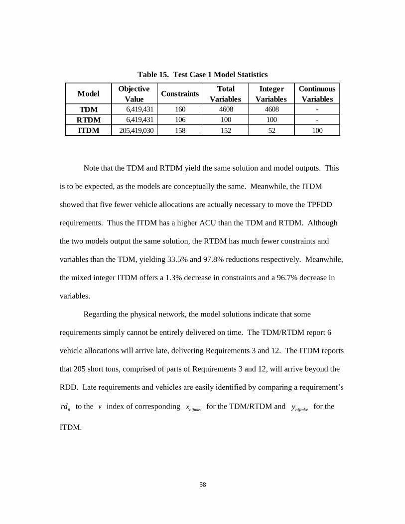
58

Table 15. Test Case 1 Model Statistics

Note that the TDM and RTDM yield the same solution and model outputs. This

is to be expected, as the models are conceptually the same. Meanwhile, the ITDM

showed that five fewer vehicle allocations are actually necessary to move the TPFDD

requirements. Thus the ITDM has a higher ACU than the TDM and RTDM. Although

the two models output the same solution, the RTDM has much fewer constraints and

variables than the TDM, yielding 33.5% and 97.8% reductions respectively. Meanwhile,

the mixed integer ITDM offers a 1.3% decrease in constraints and a 96.7% decrease in

variables.

Regarding the physical network, the model solutions indicate that some

requirements simply cannot be entirely delivered on time. The TDM/RTDM report 6

vehicle allocations will arrive late, delivering Requirements 3 and 12. The ITDM reports

that 205 short tons, comprised of parts of Requirements 3 and 12, will arrive beyond the

RDD. Late requirements and vehicles are easily identified by comparing a requirement’s

nrd to the v index of corresponding nijmkvx for the TDM/RTDM and

nijmkvy for the

ITDM.

ModelObjective

ValueConstraints

Total

Variables

Integer

Variables

Continuous

Variables

TDM 6,419,431 160 4608 4608 -

RTDM 6,419,431 106 100 100 -

ITDM 205,419,030 158 152 52 100

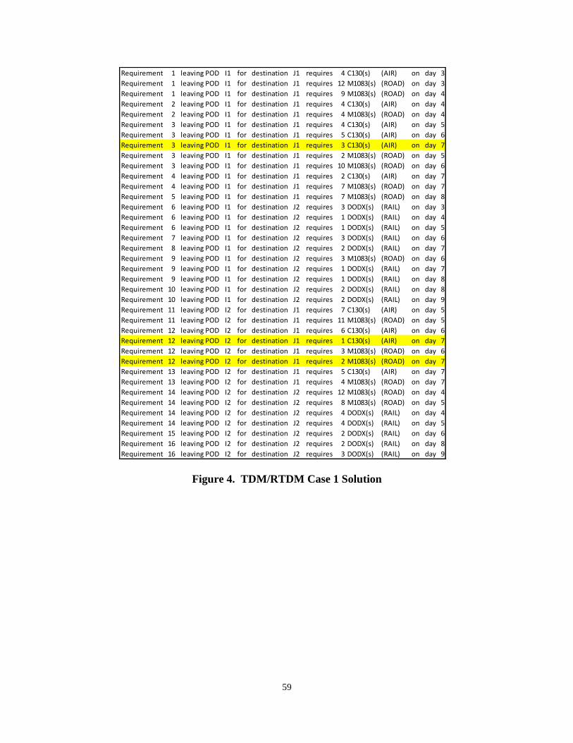
59

Figure 4. TDM/RTDM Case 1 Solution

Requirement 1 leaving POD I1 for destination J1 requires 4 C130(s) (AIR) on day 3

Requirement 1 leaving POD I1 for destination J1 requires 12 M1083(s) (ROAD) on day 3












Requirement 6 leaving POD I1 for destination J2 requires 3 DODX(s) (RAIL) on day 3

























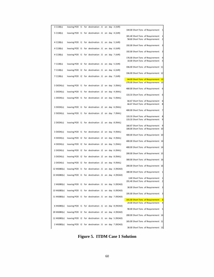
60

Figure 5. ITDM Case 1 Solution

3 C130(s) leaving POD I1 for destination J1 on day 3 (AIR)

144.00 Short Tons of Requirement 1


















3 DODX(s) leaving POD I1 for destination J2 on day 3 (RAIL)



























12 M1083(s) leaving POD I1 for destination J1 on day 3 (ROAD)




















61

Figure 4 shows the vehicle allocations determined by the model by parsing

through the nonzero decision variables and their indices. In the RTDM solution, each

requirement is allocated a number of different vehicles. In the ITDM solution, vehicle

allocations are made to POD Destination pairs for specific days which support the

delivery of different requirements. Figure 5 demonstrates this principal with the vehicle

allocations on the left-hand side and the different requirements the model has allocated to

flow on those vehicles on the right-hand side.

Test Case 2.

The second test case utilized a modified version of the TPFFD utilized in Test

Case 1. The Case 2 TPFDD is shown below in Table 16. The difference between the

two TPFDDs is a result of two distinct changes. Firstly, the short tonnage for each

requirement has been set to 1 short ton. Secondly, delivery windows were constructed

such that an intersection of at least one day exists for requirements within each

POD/Destination pair. For example, notice that Requirements 1 through 5 all are to be

delivered from 1i to 1j and each requirement could be delivered on-time on Day 6.

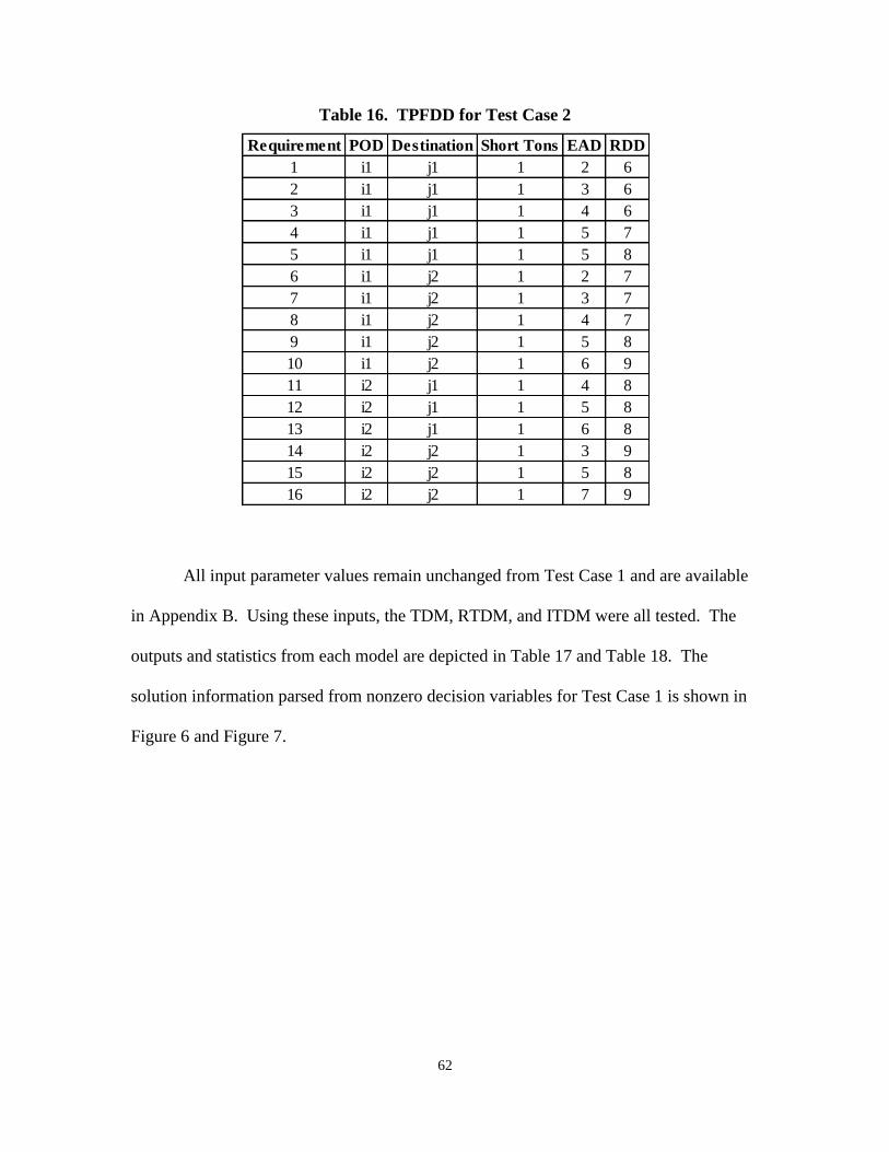
62

Table 16. TPFDD for Test Case 2

All input parameter values remain unchanged from Test Case 1 and are available

in Appendix B. Using these inputs, the TDM, RTDM, and ITDM were all tested. The

outputs and statistics from each model are depicted in Table 17 and Table 18. The

solution information parsed from nonzero decision variables for Test Case 1 is shown in

Figure 6 and Figure 7.

Requirement POD Destination Short Tons EAD RDD

1 i1 j1 1 2 6

2 i1 j1 1 3 6

3 i1 j1 1 4 6

4 i1 j1 1 5 7

5 i1 j1 1 5 8

6 i1 j2 1 2 7

7 i1 j2 1 3 7

8 i1 j2 1 4 7

9 i1 j2 1 5 8

10 i1 j2 1 6 9

11 i2 j1 1 4 8

12 i2 j1 1 5 8

13 i2 j1 1 6 8

14 i2 j2 1 3 9

15 i2 j2 1 5 8

16 i2 j2 1 7 9

63



Note that in this test case, the inherent modeling differences between the

TDM/RTDM and ITDM yield drastically different outputs. The TDM/RTDM find that

16 vehicle allocations are needed to deliver the requirements. However, the ITDM finds

that the same requirements could be delivered with only four vehicle allocations. Note

that four vehicles is the minimum allocation possible, as there are four separate

POD/Destination pairs in the TPFDD. The ITDM has the higher ACU. Regarding model

statistics, as seen in Test Case 1, both the ITDM and RTDM have greatly reduced

variables when compared to the TDM.

Model

Total

Vehicles

Allocated

Air Vehicles

Allocated

Road

Vehicles

Allocated

Rail

Vehicles

Allocated

ACU1

Late

Vehicles2

Late Short

Tons3

TDM 16 0 8 8 1.5% - N/A

RTDM 16 0 8 8 1.5% - N/A

ITDM 4 0 2 2 6.1% N/A -


2TDM and RTDM only

3ITDM only

ModelObjective

ValueConstraints

Total

Variables

Integer

Variables

Continuous

Variables

TDM 808 160 4608 4608 -

RTDM 808 106 136 136 -

ITDM 202 160 190 54 136

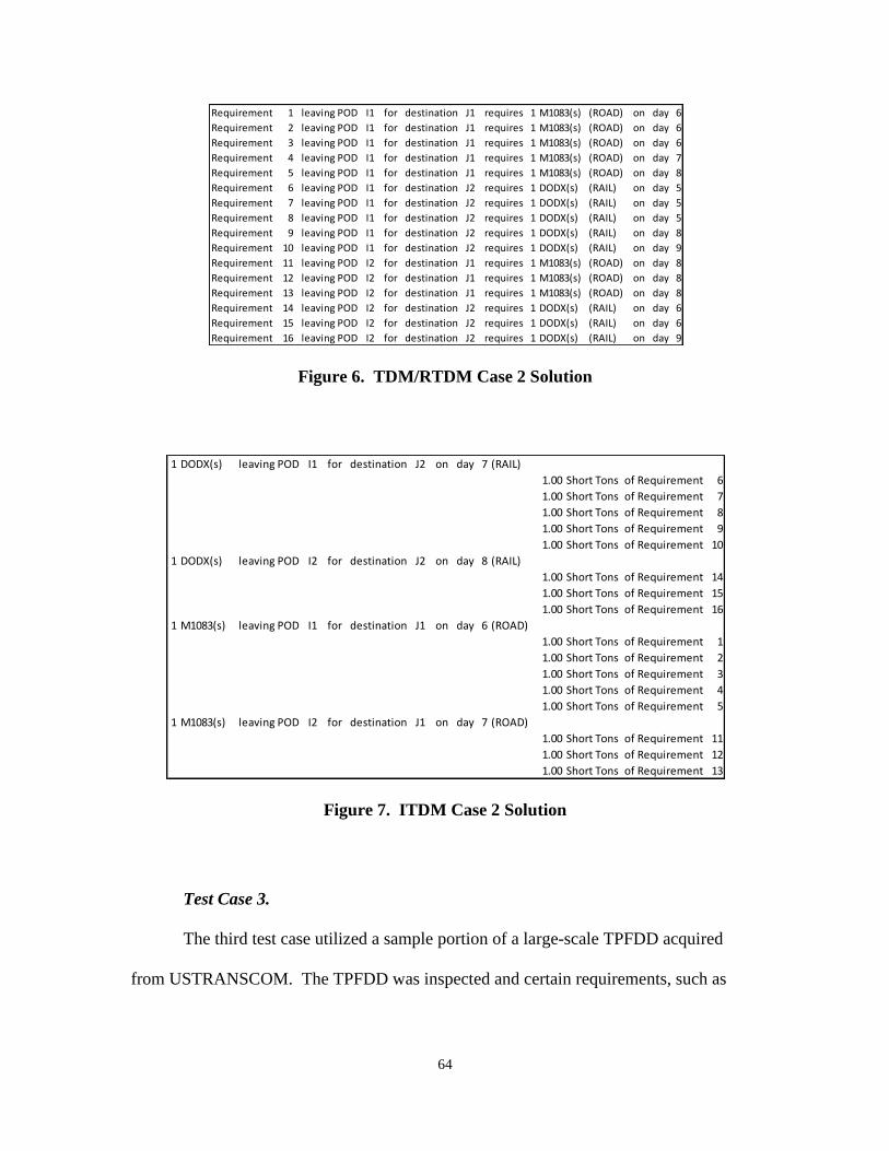
64

Figure 6. TDM/RTDM Case 2 Solution

Figure 7. ITDM Case 2 Solution

Test Case 3.

The third test case utilized a sample portion of a large-scale TPFDD acquired

from USTRANSCOM. The TPFDD was inspected and certain requirements, such as





































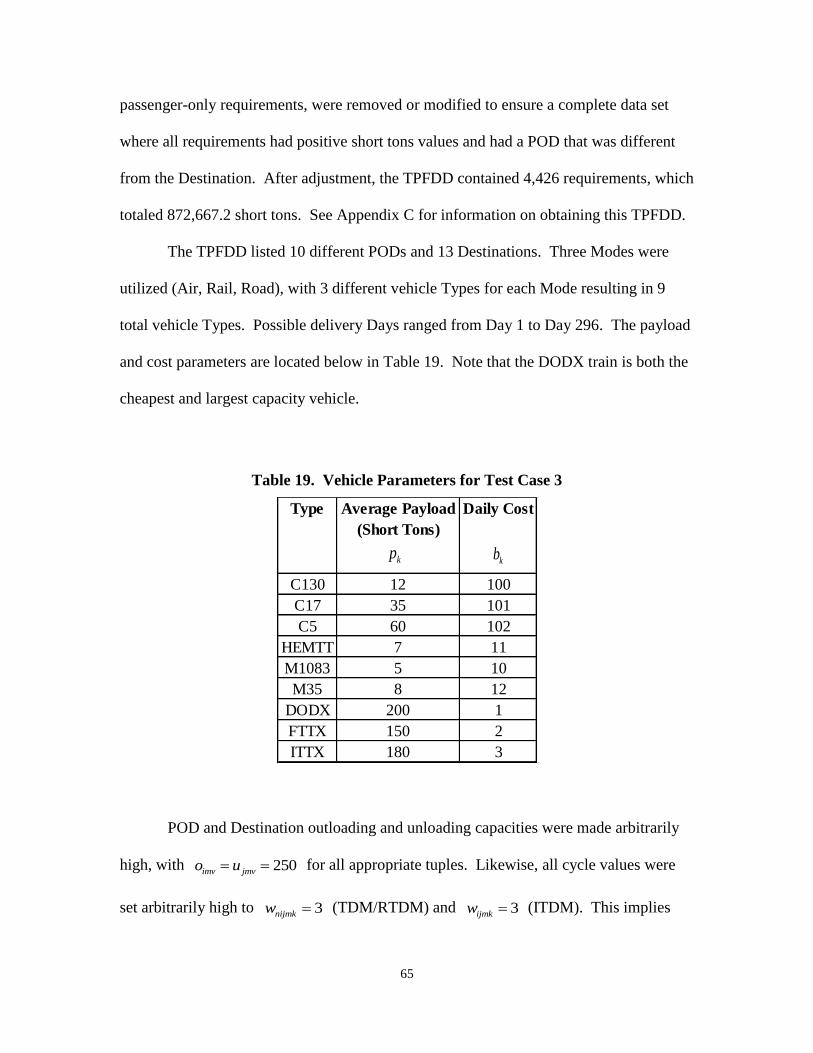
65

passenger-only requirements, were removed or modified to ensure a complete data set

where all requirements had positive short tons values and had a POD that was different

from the Destination. After adjustment, the TPFDD contained 4,426 requirements, which

totaled 872,667.2 short tons. See Appendix C for information on obtaining this TPFDD.

The TPFDD listed 10 different PODs and 13 Destinations. Three Modes were

utilized (Air, Rail, Road), with 3 different vehicle Types for each Mode resulting in 9

total vehicle Types. Possible delivery Days ranged from Day 1 to Day 296. The payload

and cost parameters are located below in Table 19. Note that the DODX train is both the

cheapest and largest capacity vehicle.

Table 19. Vehicle Parameters for Test Case 3

POD and Destination outloading and unloading capacities were made arbitrarily

high, with 250imv jmvo u for all appropriate tuples. Likewise, all cycle values were

set arbitrarily high to 3nijmkw (TDM/RTDM) and 3ijmkw (ITDM). This implies

Type Average Payload

(Short Tons)

Daily Cost

C130 12 100

C17 35 101

C5 60 102

HEMTT 7 11

M1083 5 10

M35 8 12

DODX 200 1

FTTX 150 2

ITTX 180 3

kpkb

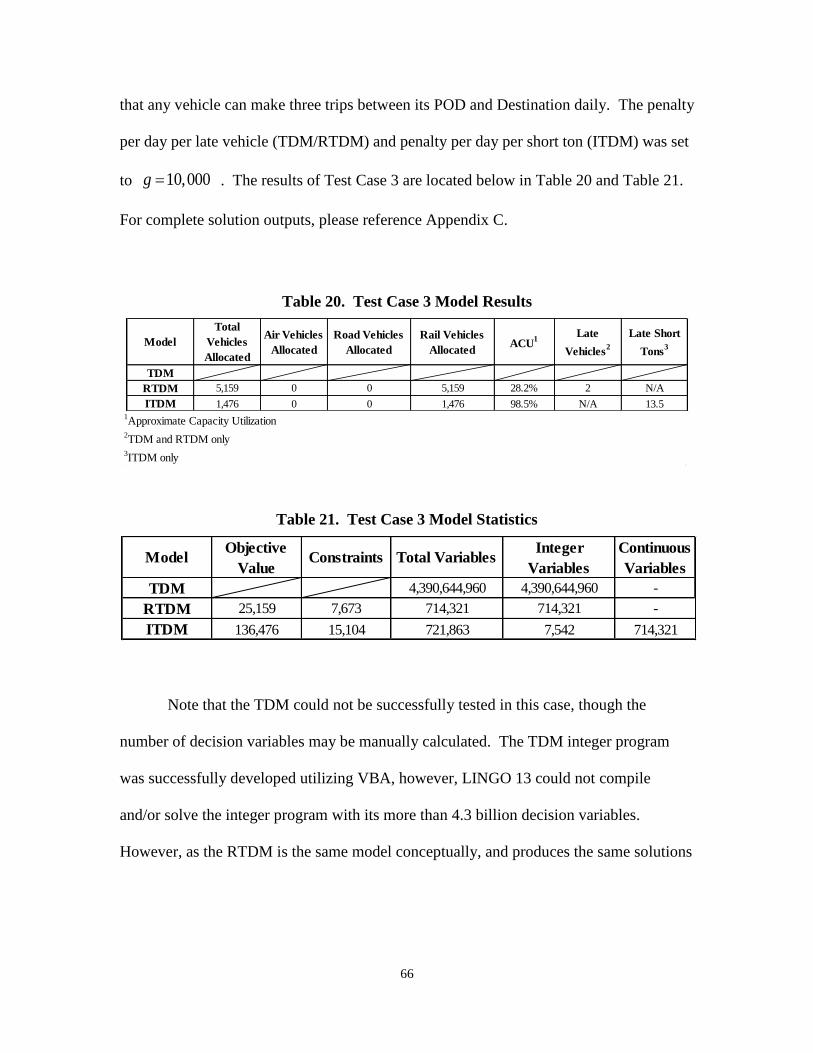
66

that any vehicle can make three trips between its POD and Destination daily. The penalty

per day per late vehicle (TDM/RTDM) and penalty per day per short ton (ITDM) was set

to 10,000g . The results of Test Case 3 are located below in Table 20 and Table 21.

For complete solution outputs, please reference Appendix C.



Note that the TDM could not be successfully tested in this case, though the

number of decision variables may be manually calculated. The TDM integer program

was successfully developed utilizing VBA, however, LINGO 13 could not compile

and/or solve the integer program with its more than 4.3 billion decision variables.

However, as the RTDM is the same model conceptually, and produces the same solutions

Model

Total

Vehicles

Allocated

Air Vehicles

Allocated

Road Vehicles

Allocated

Rail Vehicles

AllocatedACU

1Late

Vehicles2

Late Short

Tons3

TDM

RTDM 5,159 0 0 5,159 28.2% 2 N/A

ITDM 1,476 0 0 1,476 98.5% N/A 13.5

Model

Total

Vehicles

Allocated

Air Vehicles

Allocated

Road

Vehicles

Allocated

Rail

Vehicles

Allocated

ACU1

Late

Vehicles2

Late Short

Tons3

TDM 16 0 8 8 1.5% - N/A

RTDM 16 0 8 8 1.5% - N/A

ITDM 4 0 2 2 6.1% N/A -


2TDM and RTDM only

3ITDM only

ModelObjective

ValueConstraints Total Variables

Integer

Variables

Continuous

Variables

TDM 4,390,644,960 4,390,644,960 -

RTDM 25,159 7,673 714,321 714,321 -

ITDM 136,476 15,104 721,863 7,542 714,321

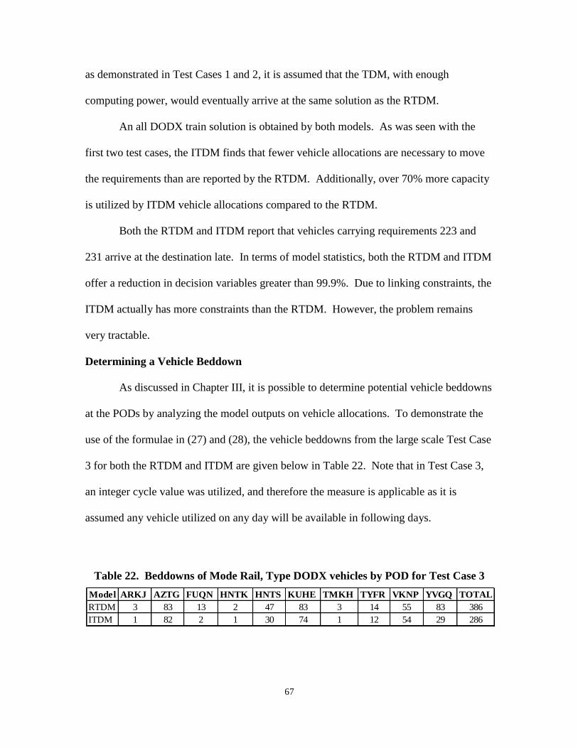
67

as demonstrated in Test Cases 1 and 2, it is assumed that the TDM, with enough

computing power, would eventually arrive at the same solution as the RTDM.

An all DODX train solution is obtained by both models. As was seen with the

first two test cases, the ITDM finds that fewer vehicle allocations are necessary to move

the requirements than are reported by the RTDM. Additionally, over 70% more capacity

is utilized by ITDM vehicle allocations compared to the RTDM.

Both the RTDM and ITDM report that vehicles carrying requirements 223 and

231 arrive at the destination late. In terms of model statistics, both the RTDM and ITDM

offer a reduction in decision variables greater than 99.9%. Due to linking constraints, the

ITDM actually has more constraints than the RTDM. However, the problem remains

very tractable.

Determining a Vehicle Beddown

As discussed in Chapter III, it is possible to determine potential vehicle beddowns

at the PODs by analyzing the model outputs on vehicle allocations. To demonstrate the

use of the formulae in (27) and (28), the vehicle beddowns from the large scale Test Case

3 for both the RTDM and ITDM are given below in Table 22. Note that in Test Case 3,

an integer cycle value was utilized, and therefore the measure is applicable as it is

assumed any vehicle utilized on any day will be available in following days.

Table 22. Beddowns of Mode Rail, Type DODX vehicles by POD for Test Case 3

Model ARKJ AZTG FUQN HNTK HNTS KUHE TMKH TYFR VKNP YVGQ TOTAL

RTDM 3 83 13 2 47 83 3 14 55 83 386

ITDM 1 82 2 1 30 74 1 12 54 29 286

68

Note that the beddowns at each POD for Mode Rail, Type DODX vehicles are

inherently larger with the RTDM than the ITDM. This follows from the fact that the

RTDM dictates more vehicle allocations than does the ITDM. Therefore, as the ITDM

projects less vehicle allocations, the beddowns are also smaller.

Limitations exist with this beddown methodology. For example, if a requirement

needs ten allocations of a certain vehicle, but has a two day window to accomplish it,

different beddowns may be derived by the model at the same cost. If all ten allocations

are made on the first day, a ten vehicle beddown would be reported. If five were made on

the first day, and five on the second day, only a five vehicle beddown would be reported

as the same five vehicles used on the first day could be used again on the second. Both

beddowns, having ten allocations, would both impact the objective function equally. In

Chapter V, ideas for further research on investigating beddowns are discussed.

Policy-Driven Solutions

To demonstrate how the models are responsive to policy changes encoded into

model parameter inputs, a slight modification was made to Test Case 3. As an example,

consider a scenario in which decision makers decide that road and rail travel will place

unnecessary harm on ground troops and air solutions are to be encouraged. Thus,

operational costs of each aircraft type could be changed to reflect this policy. In this test,

the TPFDD from Case 3 is utilized, however, some parameter inputs are modified. The

vehicle attributes were changed as shown in Table 23. Furthermore, outloading and

unloading settings were changed to 4300imv jmvo u for all appropriate tuples. Lastly,

all cycle values were updated to 43nijmkw (RTDM) and 43ijmkw (ITDM). Note

that in this test example, the C-130, an air platform, was made to have the lowest cost.

69

The higher outloading, unloading, and cycle values are arbitrary, and likely illogical, but

allow for a demonstration of an all aircraft solution.

Table 23. Vehicle Parameters for Policy-Driven Solutions Example

As a result of this setup, an all C-130 solution was obtained by both the RTDM

and ITDM (like Test Case 3, the problem was too large to compile with the TDM). This

is a direct result of the fact that C-130s were the cheapest vehicle to select for delivery.

The RTDM reported an objective of 25,241 with 5,017 C-130 allocations. The ITDM

reported an objective of 136,710 with 1,710 C-130 allocations. These results, paired with

Test Case 3, demonstrate that users can drive the model towards solutions that are

consistent with policy directives or other impacting considerations. Readers interested in

complete solutions should reference Appendix C.

Although not modeled in this research, one could easy redefine the costs such that

they are based upon attributes other than vehicle Type. For example, replacing the cost

Type Average Payload

(Short Tons)

Daily Cost

C130 12 1

C17 20 2

C5 30 3

HEMTT 7 11

M1083 5 10

M35 8 12

DODX 200 100

FTTX 150 101

ITTX 180 103

kpkb

70

kb with cost ikb would imply a separate operational cost for each POD i and vehicle

Type k combination. With this formulation, similar vehicles departing from different

PODs may be given different costs. As seen above, the model would steer towards

solutions which meet user defined objectives. If road travel out of a certain POD is

dangerous, perhaps due to Improvised Explosive Devices, road vehicles leaving this POD

could be given a higher cost than other road vehicles leaving from safer PODs. This

would require more user input. However, it is one of the many ways in which the costs

utilized in the objective value could be adapted to meet policy, guidance, or doctrine

relevant to the situation.

Aggregation

Recall from Chapter III that aggregation may be used as a precursor to

optimization. That is, aggregation of like requirements with both the same

POD/Destination pair and EAD/RDD pair may be performed. Test Cases 1 and 2 had no

such requirements. However, the aggregation of the TPFDD from Test Case 3 is

possible. To see the impact aggregation has on model outputs and statistics, the same

setup from Test Case 3 was implemented, only with the TPFDD aggregated. This

brought the number of requirements from 4,426 down to 148, although the total short

tonnage of the TPFDD remained unchanged. Table 24 and Table 25 below show the

result of the runs. For full solutions, reference Appendix C.

71

Table 24. Model Results with Aggregated TPFDD

Table 25. Model Statistics with Aggregated TPFDD

Note that with aggregation, the ITDM reports 1,476 train allocations (all of which

were DODX). This is the exact same number of DODX train allocations given by the

ITDM in the non-aggregated test run in Case 3. However, the RTDM reports a reduction

in the number of allocations, from 5,159 without aggregation to 1,547 with aggregation

even though the total short tonnage of the TPFDD remains unchanged. While

aggregation does lessen the gap between the number of allocations required between the

RTDM and ITDM, the fact that the number of allocations changes based upon

aggregation of like requirements in the RTDM is problematic. Aggregation does lead to

smaller problem size, as there are less requirements. Even so, the TDM could not

generate such a large model.

Model

Total

Vehicles

Allocated

Air Vehicles

Allocated

Road Vehicles

Allocated

Rail Vehicles

AllocatedACU

1Late

Vehicles2

Late Short

Tons3

TDM

RTDM 1,547 0 0 1,547 94.0% 1 N/A

ITDM 1,476 0 0 1,476 98.5% N/A 14


2TDM and RTDM only

3ITDM only

ModelObjective

ValueConstraints Total Variables

Integer

Variables

Continuous

Variables

TDM 153,766,080 153,766,080 -

RTDM 11,547 3,395 24,471 24,471 -

ITDM 136,476 10,862 32,013 7,542 24,471

72

In both the aggregated and nonaggregated cases, the ITDM achieved an ACU of

98.5%. However, even aggregation before optimization with the RTDM does not

achieve such an ACU. Recall that in regards to time windows, requirements are

aggregated only when there are exact matches with time windows. However, the ITDM

can allocate requirements with intersecting time windows regardless of whether

aggregation has been performed or not.

The result that the ITDM produces the same objective value for any dataset,

regardless of whether or not aggregation is done, is actually fairly straightforward. For

with aggregation, only requirements with the exact same attributes are aggregated, and

their short tonnage values are summed. Note within the ITDM, the outloading and

unloading constraints are not affected by aggregation, because nothing is indexed over

the requirements n . However, changes do occur in the objective, linking constraint, and

requirement constraint. In the objective (18), rather than summing multiple continuous

disaggregated requirement flow variables, a continuous flow variable representing

aggregated flow is in their place. Likewise, in (22) the LHS summation includes

continuous aggregated variables rather than multiple individual variables. For (19), there

are now different ( , , )n i j tuples generating constraints. The aggregated constraints

have the aggregated sum on the RHS, and on the LHS, the aggregated continuous flow

variables replace individual disaggregated variables.

Verification and Validation

As with any model, proper verification and validation must be performed as part

of the analysis. Verification seeks to ensure that one is building the model right.

73

Validation focuses on whether or not one is building the right model. These checks are

enacted upon the three models discussed in this thesis.

Verification.

Verification is conducted on each of the three models by examining the results of

Test Case 1. Firstly, as the Test Case 1inputs are drawn directly from Longhorn &

Kovich (2012), the TDM is easily verified in seeing that, within this research, the TDM

obtained the same objective value as Longhorn & Kovich did in their research. Although

alternate optimal solutions may exist, their solution was replicated. Furthermore, as the

RTDM produced the exact same output, the RTDM is verified as well. The ITDM is

verified in seeing that similar vehicle allocations were needed, although slight lower

numbers were seen due to increased ACU values. Another indication of successful

verification of the ITDM is that both the TDM/RTDM and ITDM indicated that

Requirements 3 and 12 would be delivered late, indicating the same bottleneck present in

the network.

Validation.

Test Case 2 offers one reason why the TDM and RTDM cannot be “the right

model.” Far too many vehicles are allocated to move the 16 requirements under both the

TDM and RTDM. This is what led this research to pursue an alternate modeling

technique. With the ITDM, the model avoids the issue of not being allowed to allocate

vehicles to multiple different requirements. Additionally, when examining the solutions

from all Test Cases, lower utilization rates are seen in the TDM and RTDM. This is

because the model forces at least one vehicle to be allocated to every requirement, no

matter how small. This is a poor modeling construct, and the ITDM averts this dilemma.

74

Further verification of the ITDM is not entirely possible, as results of force flow analysis

is typically classified. However, as stated above, the ITDM resolves much of the issues

seen with the TDM and RTDM.

The fact that the RTDM solutions are so sensitive to aggregation also

demonstrates it is not a useful model. Though the exact same amount of cargo needs to

be delivered with aggregation, drastic changes in solutions were seen in the aggregation

testing of the large-scale TPFDD. Conversely, the ITDM gives the same solution

whether aggregated or not because its solutions are not sensitive to the actual number of

requirements, but rather the amount of short tons in the TPFDD.

75

V. Conclusions and Future Research

Conclusions

The ITDM is the best model to use in approximating vehicle mixtures for theater

distribution. As the TDM, the baseline model, was tested and analyzed, it became quite

clear that problem sizes would be too large for real world problems. Thus, the RTDM

was developed, which solved the problem the same way but only considered relevant

decision variables and constraints. However, this reduced model still had deficiencies in

how requirements were allocated to vehicles, and thus the ITDM was developed to

address this.

The ITDM can give force flow analysts great insight into vehicles needed for a

contingency. In terms of solution quality, the ITDM is better than the TDM/RTDM as it

more accurately allocates vehicles to requirements. The RTDM forces every requirement

to have at least one vehicle allocated to it. Even if aggregation is attempted in order to

reduce the number of requirements, the RTDM still fails to achieve the ACU that is

accomplished with the ITDM. This is because aggregation only combines requirements

with exact time window matches whereas the ITDM can allocate different requirements

on a single vehicle whenever there is an intersection in the delivery windows of the

requirements.

The ITDM is also far smaller in terms of variables and constraints when

compared to the TDM. In fact, it was seen that the TDM failed to even generate for

larger problems. Because the ITDM has both continuous and integer variables, and an

76

additional linking constraint, it is actually a larger problem than the RTDM. However,

this is a tradeoff of no consequence that results in far better solutions.

Although the ITDM gives the same solutions whether the TPFDD is aggregated

or not, keeping the TPFDD disaggregated is preferred as it keeps requirements in their

initial, disaggregated state allowing for better analysis and allowing differing extension

day values to be input by commanders during analysis. However, if computing resources

are scarce, using aggregation before solving the ITDM may be an option.

Lastly, with appropriate cycle selection, solutions may be post-processed to

determine approximate vehicle beddowns required at each POD. These approximate

vehicle beddowns can provide important answers for force flow analysts. Thus, rather

than arbitrarily selecting a vehicle beddown to test in theater distribution simulations, the

ITDM can help drive feasible solutions.

The ITDM is able to find feasible vehicle mixtures that minimize operational cost

and minimize late deliveries. Because costs are user-defined, solutions may be steered

towards vehicle mixtures that align with current policy or direction. By post-processing

solutions, insights into limitations of the physical network and potential vehicle

beddowns may be gained. While the beddown measures may be sensitive to alternate

optimal solutions, finding beddowns after analysis with the ITDM can provide strong

starting points as analysts test different vehicle mixtures as part of force flow analysis.

Through the use of the ITDM and associated Decision Support System tool, force flow

analysts should be able to provide data input, model generation, solution analysis, and

solution transfer to simulation tools much faster than current guess and check methods in

place. Force flow analysts will be able to receive insight into required vehicle mixtures

77

and beddowns as they plan contingencies. This use of ITDM to model theater

distribution has the potential to save many man-hours amongst USTRANSCOM analysts

and planners.

Future Research

There are many possible adjustments to the ITDM formulation which would

allow further modeling of operational realities. The greatest potential for bettering force

flow modeling is to investigate the best way to determine vehicle beddowns. Through

the research process, it became clear that actual vehicle beddowns at PODs may be more

useful outputs for force flow analysts than what the tested models provide which are the

minimum cost allocations of vehicles to different requirements. While this thesis

develops a methodology for measuring approximate vehicle beddowns with the ITDM,

the beddowns appear to be sensitive to alternate optimal solutions. Thus, while analysts

may find such beddowns useful as starting points in distribution analysis, better beddown

solutions may exist.

An exploration of how different objectives, including minimizing lateness,

beddown size, beddown costs, and operational costs, all impact vehicle solutions yielded

by the models should prove fruitful. Changing objectives could cause further constraints

to be introduced into the model. Tradeoffs exist within these different objectives, and

thus solutions may be impacted depending on which objectives are included, as well as

any possible weighting assigned to objectives. Investigating this multiobjective problem,

and determining which objectives and measures provide proper beddowns as needed by

USTRANSCOM is a practical next step for research.

78

Another way to improve the ITDM would be to introduce a multi-commodity

flow approach. The ITDM currently can allocate any vehicle to any requirement’s short

tons. However, in reality, there are some requirements that cannot go on certain vehicles.

For example, an M1 tank cannot fit onto M1083 truck. It could, however, be placed on a

C-17 aircraft. Information regarding the type of cargo is easily accessible on a TPFDD

and therefore, restricting which vehicles may carry each requirement could produce more

realistic solutions. TPFDDs also contain passengers (i.e. troops) that need transport into

the theater. These could also be modeled as a commodity to be allocated to passenger

vehicles.

Modeling could also be expanded to include all three legs of the distribution

process. In other words, a model could show the flow of troops and materiel from home

base to POE to POD to Destination. This would greatly increase the number of variables

and would likely require the use of heuristics.

Lastly, further research into defining cycles should be conducted. Rather than

relying on user-input, a tool could be developed to calculate the greatest circular distance

(or other measure) between a POD and Destination and then, taking into consideration

vehicle speeds, outload/unload times, and other operational capabilities, report back a

particular cycle value. Furthermore, research into how to address noninteger cycle values

should be considered. As it stands now, a noninteger cycle value gives an imprecise

location of vehicles between days.

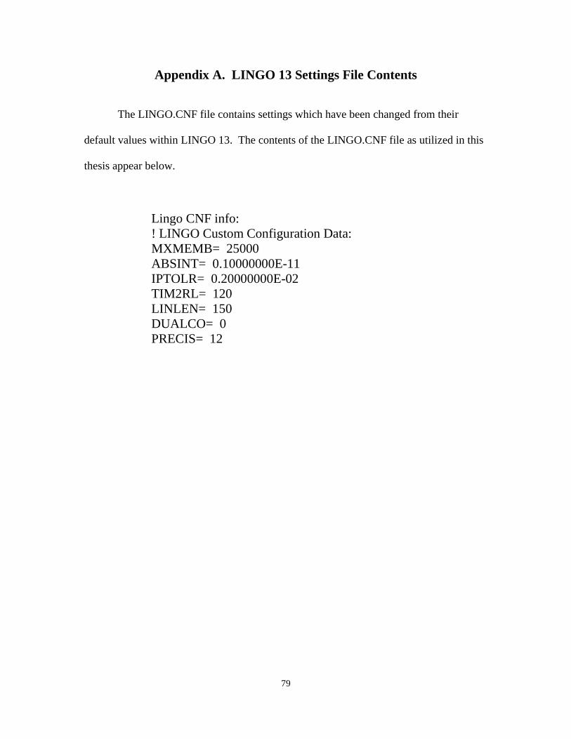
79

Appendix A. LINGO 13 Settings File Contents

The LINGO.CNF file contains settings which have been changed from their

default values within LINGO 13. The contents of the LINGO.CNF file as utilized in this

thesis appear below.

Lingo CNF info:

! LINGO Custom Configuration Data:

MXMEMB= 25000

ABSINT= 0.10000000E-11

IPTOLR= 0.20000000E-02

TIM2RL= 120

LINLEN= 150

DUALCO= 0

PRECIS= 12

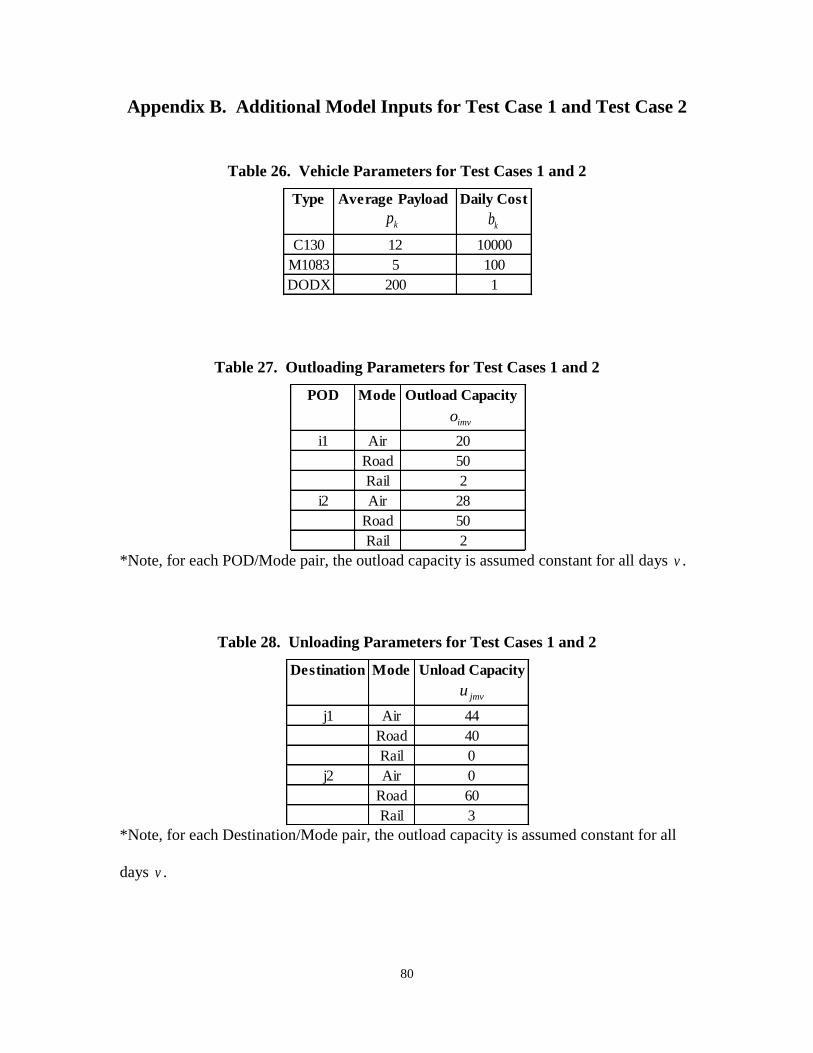
80

Appendix B. Additional Model Inputs for Test Case 1 and Test Case 2

Table 26. Vehicle Parameters for Test Cases 1 and 2

Table 27. Outloading Parameters for Test Cases 1 and 2

*Note, for each POD/Mode pair, the outload capacity is assumed constant for all days v .

Table 28. Unloading Parameters for Test Cases 1 and 2

*Note, for each Destination/Mode pair, the outload capacity is assumed constant for all

days v .

Type Average Payload Daily Cost

C130 12 10000

M1083 5 100

DODX 200 1

kpkb

POD Mode Outload Capacity

i1 Air 20

Road 50

Rail 2

i2 Air 28

Road 50

Rail 2

imvo

Destination Mode Unload Capacity

j1 Air 44

Road 40

Rail 0

j2 Air 0

Road 60

Rail 3

jmvu

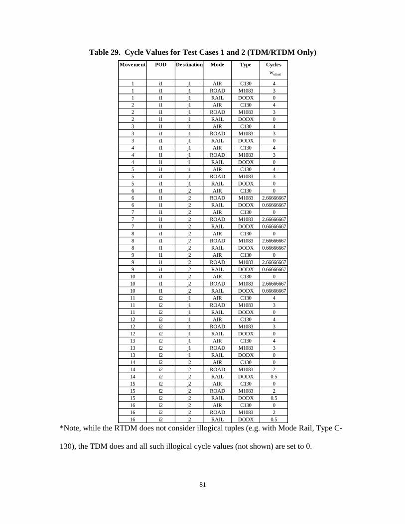
81

Table 29. Cycle Values for Test Cases 1 and 2 (TDM/RTDM Only)

*Note, while the RTDM does not consider illogical tuples (e.g. with Mode Rail, Type C-

130), the TDM does and all such illogical cycle values (not shown) are set to 0.

Movement POD Destination Mode Type Cycles

1 i1 j1 AIR C130 4

1 i1 j1 ROAD M1083 3

1 i1 j1 RAIL DODX 0

2 i1 j1 AIR C130 4

2 i1 j1 ROAD M1083 3

2 i1 j1 RAIL DODX 0

3 i1 j1 AIR C130 4

3 i1 j1 ROAD M1083 3

3 i1 j1 RAIL DODX 0

4 i1 j1 AIR C130 4

4 i1 j1 ROAD M1083 3

4 i1 j1 RAIL DODX 0

5 i1 j1 AIR C130 4

5 i1 j1 ROAD M1083 3

5 i1 j1 RAIL DODX 0

6 i1 j2 AIR C130 0

6 i1 j2 ROAD M1083 2.66666667

6 i1 j2 RAIL DODX 0.66666667

7 i1 j2 AIR C130 0

7 i1 j2 ROAD M1083 2.66666667

7 i1 j2 RAIL DODX 0.66666667

8 i1 j2 AIR C130 0

8 i1 j2 ROAD M1083 2.66666667

8 i1 j2 RAIL DODX 0.66666667

9 i1 j2 AIR C130 0

9 i1 j2 ROAD M1083 2.66666667

9 i1 j2 RAIL DODX 0.66666667

10 i1 j2 AIR C130 0

10 i1 j2 ROAD M1083 2.66666667

10 i1 j2 RAIL DODX 0.66666667

11 i2 j1 AIR C130 4

11 i2 j1 ROAD M1083 3

11 i2 j1 RAIL DODX 0

12 i2 j1 AIR C130 4

12 i2 j1 ROAD M1083 3


13 i2 j1 AIR C130 4

13 i2 j1 ROAD M1083 3


14 i2 j2 AIR C130 0

14 i2 j2 ROAD M1083 2

14 i2 j2 RAIL DODX 0.5

15 i2 j2 AIR C130 0

15 i2 j2 ROAD M1083 2


16 i2 j2 AIR C130 0

16 i2 j2 ROAD M1083 2


nijmkw

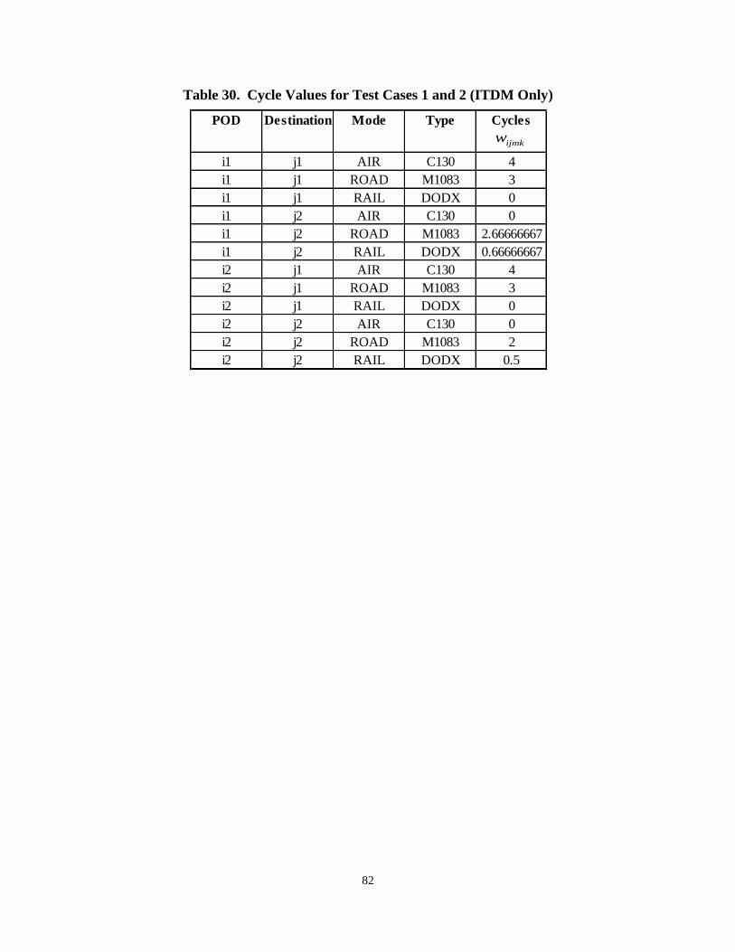
82

Table 30. Cycle Values for Test Cases 1 and 2 (ITDM Only)

POD Destination Mode Type Cycles

i1 j1 AIR C130 4

i1 j1 ROAD M1083 3

i1 j1 RAIL DODX 0

i1 j2 AIR C130 0

i1 j2 ROAD M1083 2.66666667

i1 j2 RAIL DODX 0.66666667

i2 j1 AIR C130 4

i2 j1 ROAD M1083 3

i2 j1 RAIL DODX 0

i2 j2 AIR C130 0

i2 j2 ROAD M1083 2

i2 j2 RAIL DODX 0.5

ijmkw

83

Appendix C. TPFDD and Solutions for Test Case 3

The large scale TPFDD utilized for this research contained 4,426 requirements,

resulting in a very lengthy document. Therefore, those interested in this dataset should

contact Dr. Jeff Weir, of the Air Force Institute of Technology’s Department of

Operational Sciences (AFIT/ENS). Dr. Weir can be reached at [email protected]

or at (937) 255-6565 x4523. Readers interested in seeing the complete solution outputs

should do the same.


84

Appendix D. Model Coding

The VBA coding utilized in this research to generate the RTDM and ITDM is

lengthy but available upon request. The coding of the TDM is available as well. Readers

interested in obtaining the code should contact Dr. Jeff Weir, of the Air Force Institute of

Technology’s Department of Operational Sciences (AFIT/ENS). Dr. Weir can be

reached at [email protected] or at (937) 255-6565 x4523.


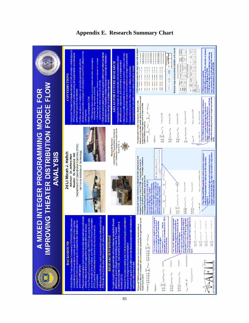
85

Appendix E. Research Summary Chart

86

Bibliography

Baldacci, R., Bartolini, E., & Mingozzi, A. (2011). An Exact Algorithm for the Pickup

and Delivery Problem with Time Windows. Operations Research, 59(2), 414-

426.

Burks, R. E., Moore, J. T., Barnes, J. W., & Bell, J. E. (2010). Solving the Theater

Distribution Problem with Tabu Search. Military Operations Research, 15(4), 5-

26.

Clark, S., Barnhart, C., & Kolitz, S. (2004). Large-scale Optimization Planning Methods

for the Distribution of United States Army Munitions. Mathematical and

Computer Modelling, 39(6-8), 697-714.

Cordeau, J., Laporte, G., Potvin, J., & Savelsbergh, M. W. (2007). Chapter 7

Transportation on Demand. In C. Barnhart, & G. Laporte (Eds.), Transportation

(p. 429). Amsterdam: North-Holland.

Crino, J. R., Moore, J. T., Barnes, J. W., & Nanry, W. P. (2004). Solving the Theater

Distribution Vehicle Routing and Scheduling Problem Using Group Theoretic

Tabu Search. Mathematical and Computer Modelling, 39(6-8), 599-616.

Dumas, Y., Desrosiers, J., & Soumis, F. (1991). The Pickup and Delivery Problem with

Time Windows. European Journal of Operational Research, 54(1), 7-22.

Ehrgott, M. (2010). Multicriteria Optimization (2nd ed.). Heidelberg: Springer.

Engels, D. W. (1978). Alexander the Great and the Logistics of the Macedonian Army.

Berkeley: University of California.

Haghani, A., & Oh, S. (1996). Formulation and Solution of a Multi-commodity, Multi-

modal Network Flow Model for Disaster Relief Operations. Transportation

Research Part A: Policy and Practice, 30(3), 231-250.

Joint Chiefs of Staff. (2008). Joint Logistics. Joint Publication 4-0. Washington: JCS.

Joint Chiefs of Staff. (2010). Distribution Operations. Joint Publication 4-09.

Washington: JCS.

Joint Chiefs of Staff. (2011). Joint Operation Planning. Joint Publication 5-0.

Washington: JCS.

Joint Chiefs of Staff. (2011). Joint Operations. Joint Publication 3-0. Washington: JCS.

Lindo Systems Inc. (2012). Lingo 13.0 (Version 13.0.2.17) [Software]. Retrieved from

http://www.lindo.com

87

Longhorn, D., & Kovich, J. (2012). Solving the Theater Distribution Problem Using

Planning Factor and Integer Programming Approaches. Scott AFB: Author.

Lu, Q., & Dessouky, M. (2004). An Exact Algorithm for the Multiple Vehicle Pickup and

Delivery Problem. Transportation Science, 38(4), 503-514.

McKinzie, K., & Barnes, J. W. (2004). A Review of Strategic Mobility Models

Supporting the Defense Transportation System. Mathematical and Computer

Modelling, 39(6-8), 839-868.

Nanry, W. P., & Barnes, J. W. (2000). Solving the Pickup and Delivery Problem with

Time Windows Using Reactive Tabu Search. Transportation Research Part B:

Methodological, 34(2), 107-121.

Rappoport, H. K., Levy, L. S., Toussaint, K., & Golden, B. L. (1994). A Transportation

Problem Formulation for the MAC Airlift Planning Problem. Annals of

Operations Research, 50, 505-523.

Rink, K. A., Rodin, E. Y., Sundarapandian, V., & Redfern, M. A. (1999). Routing Airlift

Aircraft by the Double-Sweep Algorithm. Mathematical and Computer

Modelling, 30(5-6), 133-147.

Rosenthal, R., Baker, S., Weng, L., Fuller, D., Goggins, D., Toy, A., . . . Morton, D.

(1997). Application and Extension of the Thruput II Optimization Model for

Airlift Mobility. Military Operations Research, 3(2), 55-74.

Savelsbergh, M. W., & Sol, M. (1995). The General Pickup and Delivery Problem.

Transportation Science, 29(1), 17-29.

Xu, H., Chen, Z., Rajagopal, S., & Arunapuram, S. (2003). Solving a Practical Pickup

and Delivery Problem. Transportation Science, 37(3), 347-364.

88

Vita

After graduating from Potomac Senior High School in Woodbridge, Virginia,

Lieutenant Micah J. Hafich enrolled at Virginia Polytechnic Institute and State University

in Blacksburg, Virginia, where he was a member of the Virginia Tech Corps of Cadets.

In May 2011, he earned his Bachelor of Science degree in Mathematics along with a

minor in Leadership Studies. Lieutenant Hafich was commissioned through Virginia

Tech AFROTC Detachment 875 and was recognized as a Distinguished Graduate. For

his first assignment, Lieutenant Hafich was selected to enter the Graduate School of

Engineering and Management, Air Force Institute of Technology to pursue a Master’s

Degree in Operations Research. Upon graduation, he will be assigned to the Studies and

Analysis Division at Headquarters Air Force Materiel Command (HQ AFMC/A9A),

located at Wright Patterson AFB, OH.

REPORT DOCUMENTATION PAGE Form Approved

OMB No. 074-0188

The public reporting burden for this collection of information is estimated to average 1 hour per response, including the time for reviewing instructions, searching existing data sources, gathering and maintaining the data

needed, and completing and reviewing the collection of information. Send comments regarding this burden estimate or any other aspect of the collection of information, including suggestions for reducing this burden to

Department of Defense, Washington Headquarters Services, Directorate for Information Operations and Reports (0704-0188), 1215 Jefferson Davis Highway, Suite 1204, Arlington, VA 22202-4302. Respondents should be

aware that notwithstanding any other provision of law, no person shall be subject to an penalty for failing to comply with a collection of information if it does not display a currently valid OMB control number.

PLEASE DO NOT RETURN YOUR FORM TO THE ABOVE ADDRESS.

1. REPORT DATE (DD-MM-YYYY)

27-02-2013 2. REPORT TYPE

Master’s Thesis 3. DATES COVERED (From – To)

Sep 2012 - Mar 2013 4. TITLE AND SUBTITLE

A Mixed Integer Programming Model for Improving Theater

Distribution Force Flow Analysis

5a. CONTRACT NUMBER

5b. GRANT NUMBER

5c. PROGRAM ELEMENT NUMBER

6. AUTHOR(S)

Micah J. Hafich, Second Lieutenant, USAF

5d. PROJECT NUMBER

JON 13S141 5e. TASK NUMBER

5f. WORK UNIT NUMBER

7. PERFORMING ORGANIZATION NAMES(S) AND ADDRESS(S)

Air Force Institute of Technology

Graduate School of Engineering and Management (AFIT/EN)

2950 Hobson Street

WPAFB OH 45433-7765

8. PERFORMING ORGANIZATION

REPORT NUMBER

AFIT-ENS-13-M-05

9. SPONSORING/MONITORING AGENCY NAME(S) AND ADDRESS(ES)

United States Transportation Command

Joint Distribution Process Analysis Center

Attn: Amy Pappas

508 Scott Drive DSN: 770-7758

Scott Air Force Base, IL 62225-5357 [email protected]

10. SPONSOR/MONITOR’S ACRONYM(S)

USTRANSCOM/TCAC

11. SPONSOR/MONITOR’S REPORT

NUMBER(S)

12. DISTRIBUTION/AVAILABILITY STATEMENT


13. SUPPLEMENTARY NOTES

This material is declared a work of the U.S. Government and is not subject to copyright protection in the United

States. 14. ABSTRACT

Obtaining insight into potential vehicle mixtures that will support theater distribution, the final leg of military distribution, can be a challenging and time

consuming process for United States Transportation Command (USTRANSCOM) force flow analysts. The current process of testing numerous different

vehicle mixtures until separate simulation tools demonstrate feasibility is iterative and overly burdensome. Improving on existing research, a mixed integer

programming model was developed to allocate specific vehicle types to delivery items, or requirements, in a manner that would minimize both operational

costs and late deliveries. This gives insight into the types and amounts of vehicles necessary for feasible delivery and identifies possible bottlenecks in the

physical network. Further solution post-processing yields potential vehicle beddowns which can then be used as approximate baselines for further

distribution analysis. A multimodal, heterogeneous set of vehicles is used to model the pickup and delivery of requirements within given time windows. To

ensure large scale problems do not become intractable, precise set notation is utilized within the mixed integer program to ensure only necessary variables

and constraints are generated.

15. SUBJECT TERMS

Mixed Integer Programming, Theater Distribution, Math Programming, Pickup and Delivery with Time

Windows

16. SECURITY CLASSIFICATION OF: 17. LIMITATION OF

ABSTRACT

UU

18. NUMBER

OF

PAGES

102

19a. NAME OF RESPONSIBLE PERSON

Dr. Jeffrey Weir (ENS)

a. REPORT

U

b. ABSTRACT

U

c. THIS PAGE

U

19b. TELEPHONE NUMBER (Include area code) (937) 255-6565, x4523 [email protected]

Standard Form 298 (Rev. 8-98) Prescribed by ANSI Std. Z39-18

a mixed integer programming model for improving theater

Documents