a methodology for the simulation of internal control systems

A METHODOLOGY FOR THE SIMULATION OF INTERNALCONTROL SYSTEMS

Carl Maynard Pon

LD

onterey, Galiforni

Po—

—

A METHODOLOGY FOR THE SIMULATION

OF INTERNAL CONTROL

by

SYSTEMS

Carl Maynard Pon

June 1974

Th esis AdvisMKIIUMWWl

or

:

David C. Bin

Approved for public release; distribution unlimited.

T161739

SECURITY CLASSIFICATION OF THIS PAGE (When Data Izntered)

REPORT DOCUMENTATION PAGE READ INSTRUCTIONSBEFORE COMPLETING FORM

1. REPORT NUMBER 2. GOVT ACCESSION NO. 3. RECIPIENT'S CATALOG NUMBER

4. TITLE (and Subtitle)

A METHODOLOGY FOR THE SIMULATION

OF INTERNAL CONTROL SYSTEMS

5. TYPE OF REPORT ft PERIOD COVEREDMaster's ThesisJune 19746. PERFORMING ORG. REPORT NUMBER

7. AUTHORf*;

\Carl Maynard Pon

B. CONTRACT OR GRANT NUMBER(»;

9. PERFORMING ORGANIZATION NAME AND ADDRESS

Naval Postgraduate SchoolMonterey, California 93940

10. PROGRAM ELEMENT, PROJECT, TASKAREA ft WORK UNIT NUMBERS

II. CONTROLLING OFFICE NAME AND ADDRESS


12. REPORT DATE

June 197413. NUMBER OF PAGES

73U. MONITORING AGENCY NAME ft ADDRESSfU different from Controlling O(ilce)


IS. SECURITY CLASS, (ol thla report)

Unclassified15a. DECLASSIFI CATION/ DOWN GRADING

SCHEDULE

16. DISTRIBUTION STATEMENT (ot this Report)

Approved for public release; distribution unlimited.

17. DISTRIBUTION STATEMENT (of the abstract entered in Block 20, if different from Report)

18. SUPPLEMENTARY NOTES

19. KEY WORDS (Continue on reverae aido if necaaaary and Identify by block number)

Computer Simulation; Inventory Accounting Systems;

Internal Control; SIMSCRIPT II. 5

20. ABSTRACT (Continue on roveno mlde if t\ccn»timry aid Identity by block number)

This thesis illustrates a methodology for the simulationof internal control systems. The methodology is applied toan inventory accounting system, which was the subject of thedoctoral dissertation of David C. Burns, to provide a quanti-tative measure of the adequacy of internal control . Themethodology consists of conceptualizing errors in a generalmanner and describing these errors in routines. A computer

0D | j°nM73 1473 EDITION OF 1 NOV 65 IS OBSOLETE

(Page 1) S/N 0103-014-6601I

'.iECUniTY CLASSIFICATION ol 'i HIS PAGE (KJicm Dole r.ttter: >

CtCUHITY CLASSIFICATION OF THIS PAGEfWhan Dala Entnttd)

Block 20 - ABSTRACT (Cont.)

program is then constructed which calls these routines tosimulate the error processes of the internal control systembeing modeled. The thesis includes a discussion of the suit-ability and practicability of SIMSCRIPT II. 5 to the simula-tion of internal control systems and also discusses someissues which must be resolved before it will be possible todevelop basic requirements for a simulation language special-ly designed for the simulation of internal control systems.

DD Form 1473 (BACK)i Jan 7:i

,

S/N 01 02- 01<1 -()()()! SECURITY CLASSIFICATION OF THIS PAOEfWi*" '•>•<• BnlaracO

A Methodology for the Simulation

of Internal Control Systems

by

Carl Maynard ,PonLieutenant (junior grade), United States Naval Reserve

B.A. , University of California, Los Angeles, 1972

Submitted in partial fulfillment of therequirements for the degree of

MASTER OF SCIENCE IN MANAGEMENT

from the

NAVAL POSTGRADUATE SCHOOLJune 1974

ABSTRACT

This thesis illustrates a methodology for the simulation

of internal control systems. The methodology is applied to

an inventory accounting system, which was the subject of the

doctoral dissertation of David C. Burns, to provide a quanti-

tative measure of the adequacy of internal control. The

methodology consists of conceptualizing errors in a general

manner and describing these errors in routines. A computer

program is then constructed which calls these routines to

simulate the error processes of the internal control system

being modeled. The thesis includes a discussion of the

suitability and practicability of SIMSCRIPT II. 5 to the sim-

ulation of internal control systems and also discusses some

issues which must be resolved before it will be possible to

develop basic requirements for a simulation language spe-

cially designed for the simulation of internal control sys-

tems.

TABLE OF CONTENTS

I. INTRODUCTION 9

A. GENERAL 9

1. Importance of Adequate Internal Control 9

2. Definition of Adequate Internal Control 9

3. Problem of Assessing Adequacy 11

4. Need for Objective Evaluation Methods 12

B. PURPOSE 13

1. Methodology for Simulating Internal Control 13

2. Suitability and Practicability of SIMSCRIPT 14

3. Basic Requirements for an Internal Control

Simulation Language 14

C. METHOD 15

1. Model an Inventory Accounting and Control

System 15

2. Conceptualize Errors in a General Manner — 15

3. Describe Routines in SIMSCRIPT 15

4. Write Main Program Calling Routines 16

5. Compare New Program with Original Program - 16

II. ORIGINAL SIMULATION MODEL DESCRIPTION 17

A. THE HYPOTHETICAL FIRM 17

1. General 17

2. Internal Control Weaknesses IS

3. Errors Introduced to Accounting Records 18

B. THE SIMULATION MODEL 21

1. Components 21

a. Framework 21

b. Input Generators 21

c. Erroneous Accounting Operations 21

d. Parameters 22

2. Operating Characteristics 22

III. REVISED SIMULATION MODEL DESCRIPTION 24

A. THE HYPOTHETICAL FIRM 24

1. General 24

2. Detailed Description of Error Processes 26

a. Receiving and Inspection Count Error — 26

b. Raw Material Receipts Pricing Error 26

c. Raw Material Requisitions Pricing Error 27

d. Department I Production Count Error 28

e. Department II Production Count Error — 28

f. Standard Direct Labor Hours Rate Error- 29

g. Burden Rate Error 29

h. Labor Rate Error 30

i. Production Order Transfer Rate Error — 31

3. Detailed Description of Error Correction

Process 31

B. THE SIMULATION MODEL 34

1. Components 34

a. Framework 34

b. Input Generators 36

c. Erroneous Accounting Operations 36

(1) Routine ERR0R1 36

(2) Routine ERR0R2 37

(3) Routine ERR0R3 3S

6

d. Parameters 39

2. Output Comparison 39

IV. SUITABILITY AND PRACTICABILITY OF SIMSCRIPT 43

A. REASON FOR USING SIMSCRIPT 43

B. SUITABILITY OF SIMSCRIPT 45

1. Strengths of SIMSCRIPT 45

2. Weaknesses of SIMSCRIPT 46

3. Assessment of Suitability 47

C. PRACTICABILITY OF SIMSCRIPT 48

1. Strengths of SIMSCRIPT 48

2. Weaknesses of SIMSCRIPT 48

3. Assessment of Practicability 49

D. FINAL ASSESSMENT OF SIMSCRIPT 50

V. SUMMARY AND CONCLUSION 52

A. METHODOLOGY FOR SIMULATING INTERNAL CONTROL 52

1. Success of Revised Methodology 52

2. Extension of Revised Methodology 53

B. FEASIBILITY OF USING SIMSCRIPT 54

C. ISSUES TO BE RESOLVED 55

1. Optimal Size System to Simulate 55

2. Conceptualization of Errors 56

3. Conceptualization of Controls 57

4. Structure of Input Data 59

D. FINAL REMARKS 60

APPENDIX A Operational Flow Chart of Revised Model 61

COMPUTER PROGRAM 67

LIST OF REFERENCES 72

INITIAL DISTRIBUTION LIST 73

7

LIST OF FIGURES

1. Standard Cost Build-Up 19

2. Distributions and Ceilings Used by Input Data

Generators 25

3. Standards for Production Costing: Correct and

Erroneous 32

4. Output of Original and Revised Simulation Models 40

8

I. INTRODUCTION

A. GENERAL

1

.

Importance of Adequate Internal Control

The existence of adequate internal control is essen-

tial to the management of any enterprise. The importance of

internal control is due to the fact that almost every type

of business decision involves accounting data to some extent.

Adequate internal control assures management that the account-

ing data used in making decisions is reasonably accurate.

In addition, internal control promotes operational compliance

with business decisions that are established as policy.

Adequate internal control is equally important to an

external- auditor. The adequacy of internal control is the

most important factor in determining the nature of the audi-

tor's examination. This statement can be supported by the

fact that generally accepted auditing standards require an

auditor to perform a study and evaluation of internal con-

trol before he determines the auditing procedures necessary

to formulate an opinion on the fairness of financial state-

ments.

2

.

Definition of Adequate Internal Control

The definition of internal control used in this

thesis is the definition implicitly used by the Committee on

Auditing Procedure: ".. . the plan of organization and the

procedures and records that are concerned with the

safeguarding of assets and the reliability of financial re-

cords. . ." The definition continues with mention that in-

ternal control should provide "reasonable assurance" that

internal control will achieve its objectives. This concept

recognizes that the cost of internal control should not be

greater than the benefit it provides. It should be noted

that the above definition of "internal control" actually

describes a system of internal control. In this thesis the

phrase "internal control" is synonymous with "system of in-

ternal control."

When an auditor evaluates how adequate internal con-

trol is, he concentrates on the extent to which internal

control prevents or detects material errors and irregular-

ities in the financial statements. The criteria used to

determine whether or not internal control is adequate is the

presence or absence of a material weakness in the system.

Quoting the Committee on Auditing Procedure:

In this context, a material weakness meansa condition in which the auditor believes the pre-scribed procedures or the degree of compliance withthem does not provide reasonable assurance that er-rors or irregularities in amounts that would be ma-terial in the financial statements being auditedwould be prevented or detected within a timely per-iod by employees in the normal course of performingtheir assigned functions.

Committee on Auditing Procedure, Statement on AuditingStandards No. 1

, p. 20, American Institute of Certified Pub-lic Accountants, Inc., 1973.

2Lbid . , p. 30.

.10

3. Problem of Assessing Adequacy

According to the Committee on Auditing Procedure,

the auditor should assess the adequacy of internal control

using the following four step process:

a. Consider the types of errors and irregulari-ties that could occur.

b. Determine the accounting control proceduresthat should prevent or detect such errorsand irregularities.

c. Determine whether the necessary proceduresare prescribed and are being followed satis-factorily .

d. Evaluate any weaknesses— i.e., types of po-tential errors and irregularities not coveredby existing control procedures—to determinetheir effect on (1) the nature, timing or ex-tent of auditing procedures to be applied and(2) suggestions to be made to the client.^

The problem which faces the auditor is that the

assessment process must consider the interaction of a multi-

tude of people, processes, and procedures. The auditor is

required to estimate acceptable error rates and error magni-

tudes for each person, process, and procedure connected with

internal control. These acceptable error rates are used as

a basis for determining upper precision limits for statisti-

cal sampling tests which are intended to determine the actual

rates. To derive these acceptable error rates and magnitudes,

the auditor must assess their net affect on the accounting

system. The more extensive the system of internal control

is, the more complex such mental assessments become.

For a large enterprise, such as a Naval Supply Cen-

ter, internal control systems are so extensive that it is

3Ibid . , pp. 31-32

11

difficult to follow even one transaction through the system.

Consequently, when it is necessary to consider the numerous

transactions which occur over an extended period of time,

mental assessment becomes extremely difficult, especially if

offsetting or compound errors are possible. Since evaluation

of internal control requires the auditor to consider the en-

tire system instead of just individual errors, it can be

seen that mental assessment becomes a hopelessly complex

problem.

4. Need for Objective Evaluation Methods

Because of the difficulty of evaluating an entire

system of internal control, the auditor may instead choose

to evaluate subsystems of internal control. An example of

such a subsystem would be all controls related to an inven-

tory account. When acceptable error rates are established

for a subsystem, a two-step evaluation is normally performed.

First, each control is assessed separately with regard to

acceptable error rates and magnitudes. Second, the net ef-

fect of all the individual acceptable error rates upon the

accounting system is subjectively determined. If this net

error is too large, the auditor may have to repeat the first

step.

At present, auditors do not use any type of objective

method to assist them in assessing the adequacy of an inter-

nal control subsystem. Consequently, the more complex the

subsystem, the less confidence the auditor can place in his

subjective assessment. This fact has been established by

12

at least one experiment which showed that even with perfect

knowledge of error rates an auditor could not make an accu-

rate subjective assessment of internal control with respect

4to inventory account balances. This experiment illustrated

a need for quantitative or objective methods of evaluating

internal control which is also expressed in a forthcoming

5article by John Neter and Seongjae Yu.

B . PURPOSE

1. Methodology for Simulating Internal Control

The first purpose of this thesis is to illustrate

the use of a modified version of the methodology used by

Burns in his doctoral dissertation, with the intent of sim-

plifying the writing of a computer program for a simulation

model of internal control. The methodology used by Burns

was essentially to begin from scratch: the internal control

system of a hypothetical firm was first simplified and then

described by a computer program which defined each error

process in this particular system. Consequently, this meth-

odology resulted in a very special-purpose model.

This thesis deals with the same system, but describes

it using a different methodology. Rather than describe each

4 David C. Burns, Audit Evidence Evaluation Using Com-puter Simulation with Special Emphasis on Ascertaining theReliability of Accounting Data , Doctoral Dissertation, Indi-ana University, Bloomington, Graduate School of Business, 1971

5 This article will appear in a forthcoming issue of TheJournal of Accounting Research

,published by the University

of Chicago.

13

individual error process as it occurs in this particular sys-

tem, error processes are described in routines which will be

called by a main program at the proper time. These routines

are so general that they require the user to specify values

for parameters which were constants in Burns' dissertation

(e.g., error rates and error magnitudes). Consequently,

these routines can be used to describe any number of inter-

nal control systems simply by changing the sequence of error

routines or by changing the values of parameters.

2. Suitability and Practicability of SIMSCRIPT

The second purpose of this thesis is to determine

both the suitability and the practicability of SIMSCRIPT as

a programming language to be used for describing simulation

models of internal control systems. The reasons for choos-

ing SIMSCRIPT rather than any other programming language are

presented later in the thesis.

3. Basic Requirements for an Internal Control Simula-

tion Language

The third purpose of this thesis is to identify the

basic requirements for a simulation language which could be

used specifically for simulation of internal control sys-

tems. Discussion of these requirements considers the basic

issues and problems which must be resolved to develop such

a language.

14

C . METHOD

1. Model an Inventory Accounting and Control System

The model presented in this thesis is based upon the

inventory accounting and control system of a hypothetical

firm which was described in the doctoral dissertation of

David Burns. The rationale for using this system is that it

presents a variety of auditing problems which are representa-

tive of the problems found in other types of internal control

subsystems. In addition, since some of the most complex

auditing problems are related to manufacturing inventories,

the argument can be made that if this system can be modeled,

any subsystem can be modeled.

2. Conceptualize Errors in a General Manner

The error processes which will be described in rou-

tines will be conceptualized in as general a manner as is

possible. This means that there will be no constants in the

error routines, only variables. As a result of this concep-

tualization, only three error routines will be needed to de-

scribe the eight error processes found in the hypothetical

system.

3. Describe Routines in SIMSCRIPT

The use of SIMSCRIPT to describe error routines is

completely independent of the manner in which the error proc-

esses are conceptualized. This means that SIMSCRIPT could

just as easily have been used to describe the hypothetical

system as originally conceptualized and that other program-

ming languages could have been used to describe the

15

conceptualization of errors in a general manner. The reason

for making this point is to emphasize that the use of SIM-

SCRIPT was an activity separate from the conceptualization

of error processes as general routines.

4. Write Main Program Calling Routines

The main program, which will simulate the inventory

accounting and control system, is an activity separate from

the description of error routines. This means that the sys-

tem described in the main program is only one of many systems

that could be described by calling the same error routines

in a different order and/or with different variable values.

5

.

Compare New Program with Original Program

The output of the "new" program (described in SIM-

SCRIPT) will be compared with those of the original model

(described in FORTRAN). This will establish the fact that

the two programs represent the same system. After this fact

is established the thesis will continue with an evaluation

of SIMSCRIPT and consideration of the issues and problems

raised by the "new" method of conceptualizing errors.

16

II. ORIGINAL SIMULATION MODEL DESCRIPTION

A. THE HYPOTHETICAL FIRM

1. General

The "original" simulation model was based on the man-

ual inventory accounting system of a hypothetical manufac-

turing firm. The processes attributed to the hypothetical

firm and its inventory accounting system were in fact ab-

stracted from those which occurred in a real business firm.

This real firm was engaged in the business of machining and

selling alloy and cast-iron pipe fittings.

Since the real firm carried a product line of over

two thousand fittings, it was necessary to restrict the

scope of this real firm when transforming it into the hypo-

thetical firm. Consequently, the hypothetical firm and the

simulation model were restricted to four products from this

total line. These four products are referred to by number,

products 1, 2, 3 and 4. Production of each of these four

products was assumed to involve two manufacturing departments,

Department I and Department II.

The financial accounting records of the hypothetical

firm carried inventories of raw materials, work-in-process,

and finished goods at predetermined standard costs. As was

A detailed description of the original simulation modelcan be found in Naval Postgraduate School Report 55Bu73111A,A Computer Simulation Case for the Auditing Classroom , b

y

David C. Burns, pp. 6-66, November 1973.

17

mentioned before, inventory accounting operations were per-

formed manually. A build-up of the standard costs for all

four products is given in Figure 1.

2. Internal Control Weaknesses

A study and evaluation of internal control performed

by an auditor on the hypothetical firm would have detected

the following weaknesses in internal control with respect to

inventories:

1) Receiving and inspection personnel were lax in

that they did not perform physical counts of incoming raw

material shipments.

2) Access to the raw material storage area was not

controlled in a prudent manner.

3) The files containing standard cost cards were

not maintained in an orderly fashion.

4) Foremen did not check the accuracy of production

counts stated by their operators.

5) The weigh-count operator was lax in verifying

the counts stated on production orders before the goods were

placed in the finished goods storage area.

3

.

Errors Introduced to Accounting Records

The internal control weaknesses described above were

further assumed to permit the following errors to affect the

hypothetical firm's inventory accounting records:

1) Shipments of raw materials received by the firm

sometimes contained more units than were stated on the ven-

dor's or shipper's invoice. The receiving and inspection

.18

FIGURE 1

STANDARD COST BUILD-UP

Product Product Product ProductNumber 1 Number 2 Number 3 Number 4

Direct Material

Type of Material R. M. 1 R. M. 2 R. M. 3 R. M. 4

Units Required 1 1 1 1

Spoilage/Scrap, <2tC.

Standard Cost of Material $13.5000 $16.7000 $ 6.5000 $ 8.000

Total/Unit $13.5000 $16.7000 $ 6.5000 $ 8.000

Direct Labor

Department I

Std dir lbr hrs/unit

Std dir lbr rate

Total std dir lbr charge

Department II


Std dir lbr rate

Total std dir lbr charge

Total/Unit

Burden

Department I

•Std dir lbr hrs/unit

Std burden rate

Total std burden charge

Department II


Std burden rate

Total std burden charge

Total Burden/Unit

Total Unit Standard Cost

.06 hr .09 hr .04 hr .06 hr

$ 6.20/hr $ 6.20/hr $ 6.20/hr $ 6.20/hr

$ .3720 $ .5580 $ .2480 $ .3720

.04 hr .06 hr .04 hr .07 hr

$ 5.60/hr $ 5.60/hr $ 5.60/hr $ 5.60 hr

$ .2240 $ .3360 $ .2240 $ .3920

5960 $ .8940 $ .4720 $ ,7640

.06 hr .09 hr .04 hr .06 hr

$12.85/hr $12.85/hr $11.40/hr $11.40/hr

$ .7710 $ 1.1565 $ .4560 $ .6840

.04 hr .06 hr .04 hr .07 hr

$51. 55/hr $51.55/hr $44.05/hr $44.05 hr

$ 3.0930 $ 1.7620 $ 3.0835

$ 4.2495 $ 2 .2180 $ 3.7675

$21.8435 $ 9.1900 $12.5315

$ 2.,0620

$ 2.,8330

sir,,,9290

Abbreviations : std =standard; dir =dircct:; ]br =labor; hrs --hours.

19

department personnel were assumed to be lax in performing

their duties. Consequently these understatements could re-

main undetected and uncorrected.

2) Lack of control over access to the raw materials

storage area allowed the unauthorized and unrecorded return

of excess raw materials which had been requisitioned to sup-

port inflated production counts.

3) Careless maintenance of standard cost files re-

sulted in the application of incorrect standard costs while

vouching raw material purchases, costing production orders,

or transferring goods from work-in-process to finished goods.

4) The laxity of foremen allowed the random over-

statements of production counts to remain undetected in both

Department I and Department II.

5) The laxity of the weigh-count operator allowed

most of the random overstatements of production counts to

pass undetected as goods were moved to the finished goods

storage area.

The error processes outlined above caused both over-

statements and understatements of the various inventory ac-

counts to be introduced into the account balances. Detailed

descriptions of these error processes are presented later in

this thesis.

20

B. THE SIMULATION MODEL

1. Components

The original computer simulation model can be de-

scribed in terms of the following components:

a. Framework

The framework of the model was a FORTRAN program

describing the inventory accounting system. Functions per-

formed by the program include vouching raw material purchases

and the costing of material requisitions, production reports,

transfers of finished goods, and sales. The program main-

tained two separate sets of inventory accounting records.

The "reported" account balances contain the net amount of

the correct balance and all errors, while the "control" ac-

count balances contain only the correct balance.

b. Input Generators

The model included several external input gener-

ators which provide the input data that is subsequently

processed by the framework. These data represent the quan-

tity of raw materials contained in raw materials shipments

and the number of units of product specified in production

orders

.

c. Erroneous Accounting Operations

The model used the Monte Carlo technique to sim-

ulate the erroneous accounting operations by causing errors

to occur at random in accordance with predefined probability

distributions. These errors had an affect only on the "re-

ported" balance, since the "control" balances reflected only

the correct portion of each transaction.

21

d. Parameters

The parameters of the model included beginning

inventory levels, files of correct and incorrect standard

costs, and quantities which limited the total volume of fi-

nancial accounting activity. The volume was controlled by

placing a ceiling on the amount of raw materials to be pur-

chased and on the amount of each product to be manufactured.

2. Operating Characteristics

The original model included a set of computer state-

ments which caused 1500 iterations of the simulation process

to be performed. This large number of iterations was neces-

sary to perform certain nonparametric goodness-of-f it sta-

tistical tests. However, one hundred iterations produced

statistics which were suitable for estimating the total er-

ror.

The model used pseudo-random numbers to trigger the

occurance of errors during the simulation process. A differ-

ent sequence of pseudo-random numbers was used during each of

the 1500 iterations of the model. Consequently, the combina-

tions of processing errors which occurred during each itera-

tion of the model were statistically independent.

In addition to calculating the total error present

in ending inventory balances at the end of each iteration,

the model was designed to plot these errors as a probability

distribution and to calculate the mean and standard deviation

of this distribution. The mean and standard deviation of

the probability distribution were quantitative measures of

22

the adequacy of internal control. Both measures were needed

since a mean of zero dollar error could still reflect inade-

quate internal control if the standard deviation were large

enough to make material errors reasonably likely.

2 a

III. REVISED SIMULATION MODEL DESCRIPTION

A. THE HYPOTHETICAL FIRM

1. General

The "revised" simulation model was based on the same

manual inventory accounting system of the hypothetical firm.

This was done so that this thesis could concentrate on the

changes in the conceptualization of the system and on the

different computer language used to describe the conceptual-

ization. However, there was one minor difference between

the original simulation model and the revised simulation mod-

el which had no effect on the operating characteristics of

the model, but is discussed for sake of completeness.

This difference between the two models is related to

the external input generators. Ceilings were established to

control the total units of raw materials to be received and

the units of each product that were to be put into process

and transferred to finished goods. The original model re-

duced the quantities of a shipment or production order which

would exceed the ceiling so that the ceiling would be met

but not exceeded. The revised model did not reduce the

quantities, so the ceiling could be slightly exceeded. How-

ever, due to the small size of individual raw material ship-

ments and production order quantities relative to these

ceilings (see Figure 2), the effect of this change on the

results of the revised model was insignificant.

24

FIGURE 2

DISTRIBUTIONS AND CEILINGS USED

BY INPUT DATA GENERATORS

Raw Raw Raw RawMaterial 1 Material 2 Material 3 Material 4

Units to be receivedduring the period

Mean of normal distri-bution of raw materialshipments

Standard deviation ofnormal distribution ofraw material shipments

40,000

200

25

34,000

180

30

34,000

200

25

32,000

180

30

Units to be placedinto process duringthe period

Units to be trans-ferred to finishedgoods during theperiod

Mean of normal dis-tribution of produc-tion orders

Standard deviationof normal distribu-tion of productionorders

Product 1 Product 2 Product 3 Product 4

33,600 33,000 33,000 28,900

30,280

150

35

30,964

150

35

29,777

150

35

21,719

150

35

25

2. Detailed Description of Error Processes

As was explained above, there was only one difference

between the hypothetical firm in the original model and that

in the revised model. It is important to emphasize this

fact to avoid any misinterpretation of the following descrip-

tions, which explain in detail the error processes found in

the hypothetical firm and used as a basis for both the orig-

inal and the revised model.

a. Receiving and Inspection Count Error

The count error which could occur during receiv-

ing and inspection operations resulted from the failure of

employees to physically count shipments received. The nature

of the error was the same for all four raw materials: each

shipment processed had a twenty-five per cent chance of being

understated by ten per cent of the correct quantity received.

b. Raw Material Receipts Pricing Error

Weak control over the standard cost file resulted

in the possibility that an incorrect standard cost for raw

materials could be applied to purchase orders. This in turn

resulted in erroneous vouchering of raw material receipts

and incorrect entries to raw materials inventory. For each

of the four raw materials, there was a ten per cent chance

that this error could occur. However, the monetary value of

the rate error was a function of the raw material which was

being vouchered. If an error occurred:

1) Raw Material 1 was priced at the standard

cost of Raw Material 3.

26







c. Raw Material Requisitions Pricing Error

Since all raw materials were put into process in

Department I, pricing errors in raw material requisitions

could occur only as a result of Department I operations.

These pricing errors were all assumed to be the result of

misfiled standard cost cards. For each of the four products

(and thus, for each of the four raw materials) there was a

ten per cent chance that such an error would occur. If an

error occurred:

1) Raw Material 1 used to produce Product 1 was

priced at the standard cost of Raw Material 3.







It should be noted that since the standard usage of material

for each product was the same and that each product only re-

quired one raw material, errors in pricing were the only er-

rors possible when processing raw material requisitions.

27

d. Department I Production Count Error

Overstatements of production counts are assumed

to occur because machine operators were paid incentive wages

and because internal control weaknesses made it possible for

such overstatements to remain undetected. These weaknesses

are due to the laxity of foremen in verifying the counts of

their subordinates and the lack of control over access to the

raw materials storage area. This lack of control made it

possible for machine operators to plan on overstating produc-

tion counts. Their method was to requisition enough material

to support their inflated production counts and later return

excess material without management's knowledge. In the hypo-

thetical firm there was assumed to be a fifteen per cent

chance that a "count error" would occur. When such an error

did occur, the quantity stated in the production order repre-

sented a ten per cent overstatement of the actual quantity.

e. Department II Production Count Error

When a production order reaches Department II,

the Department I count was always accepted as correct, even

if it was overstated. Thus it was assumed that Department II

employees in the hypothetical firm cover-up for the overstate-

ments of Department I employees. In addition, Department II

employees may overstate production counts regardless of

whether or not Department I overstated its count on a given

production order. Thus, these overstatements were independ-

ent events. The chance that a Department II employee would

overstate a production order was eight per cent, and when

28

this "count error" occurs, the result was a five per cent

overstatement of the quantity stated in the production order.

f

.

Standard Direct Labor Hours Rate Error

Weak control over the standard cost file resulted

in the possibility that an incorrect standard for the direct

labor hours to produce one unit of product could be applied

when costing a job time ticket. If an incorrect standard

was used, the "rate error" affected the application of both

burden and direct labor to the job time ticket. The chance

that such a "rate error" would occur for any product was

eight per cent. When such an error did occur:

1) The standard for Product 3 was applied to a

job time ticket for Product 1.







It should be noted that this error could occur in one, two,

or neither of the manufacturing departments.

g. Burden Rate Error

The occurrence of a burden rate error was inde-

pendent of an error in applying the standard direct labor

hour rate to a job time ticket. The chance that such an er-

ror would occur was eight per cent, and when such an error

did occur:

29

1) The burden rate for Product 3 was applied to

a job time ticket for Product 1.








or none of the manufacturing departments.

h. Labor Rate Error

The occurrence of a labor rate error was inde-

pendent of an error in applying the standard direct labor

hour rate to a job time ticket. There was assumed to be a

ten per cent chance that such an error would occur in the

hypothetical firm. When such an error did occur, there were

two possible outcomes:

1) The labor rate for last, year was applied to

the job time ticket.

2) The labor rate for the wrong manufacturing

department was applied to the job time ticket.

These two outcomes were assumed to be equally likely. That

is, each was expected to occur fifty per cent of the time.


or none of the manufacturing departments.

:;n

i. Production Order Transfer Rate Error

Each production order for each type of product

was transferred to finished goods until a specified number

of units had been transferred. Units of product transferred

to finished goods were costed at the total standard cost for

the given product. Once again, the weak control over the

standard cost file interjected a potential "rate error" into

the accounting system. The chance of such an error occurring

was eight per cent, and when this error occurred:

1) A production order for Product 1 was costed

at the standard cost of Product 3.







The standard cost relevant to this error and the errors

which have been described before it are presented in Figure

3.

3 . Detailed Description of Error Correction Process

Before the product stated on each production order

was transferred to the finished goods storage area, a weigh-

count operator verified the count stated on the production

order. However, the operator was assumed to be so lax in

performing his duties that only overstatements of twenty-one

or more units were detected. When overstatements wore

31

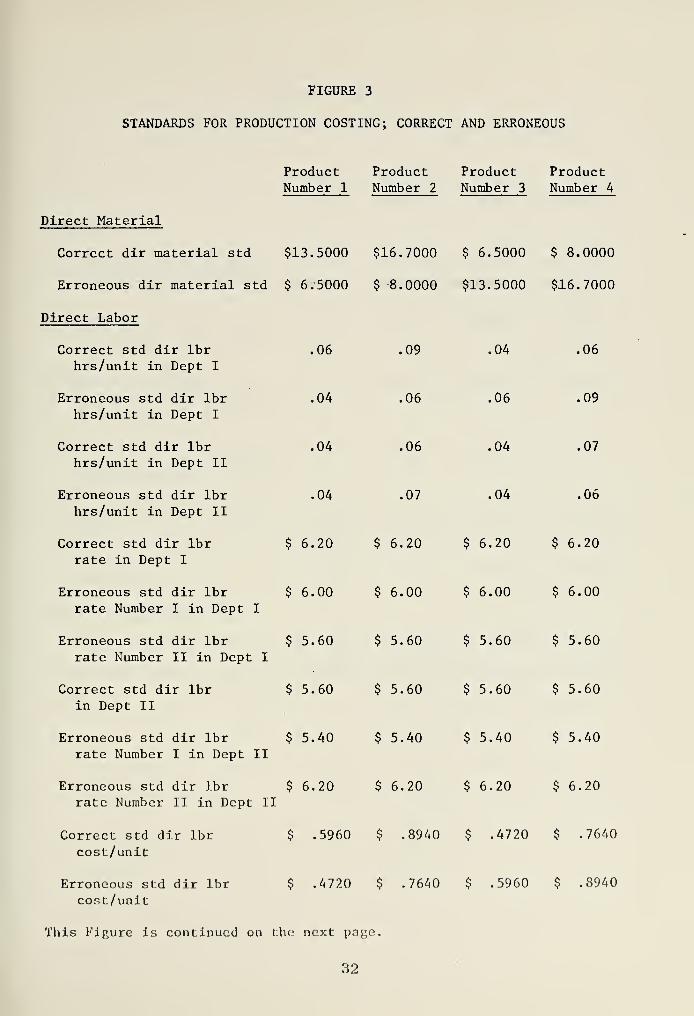
FIGURE 3

STANDARDS FOR PRODUCTION COSTING; CORRECT AND ERRONEOUS

ProductNumber 1

Direct Material

Correct dir material std $13.5000

Erroneous dir material std $ 6.5000

Direct Labor

Correct std dir lbrhrs/unit in Dept I

Erroneous std dir lbrhrs/unit in Dept I

Correct std dir lbrhrs/unit in Dept II

Erroneous std dir lbr

hrs/unit in Dept II

.06

.04

.04

.04

ProductNumber 2

$16.7000

$ 8.0000

.09

.06

.06

.07

Correct std dir lbrrate in Dept I

$ 6.20 $ 6..20

Erroneous std dir lbrrate Number I in Dept I

$ 6.00 $ 6,,00

Erroneous std dir lbrrate Number II in Dept I

$ 5.60 $ 5.,60

Correct std dir lbrin Dept II

$ 5.60 $ 5,,60

Erroneous std dir lbrrate Number I in Dept II

$ 5.40 $ 5,,40

Erroneous std dir lbrrate Number II in Dept II

$ 6.20 $ 6,,20

Correct std dir lbr

cost/unit$ .5960 $ .89

Erroneous st.d dir lbr

cost/unit$ .4720 $ .76

This Figure is continued on the next: pa ge.

Product ProductNumber 3 Number 4

$ 6.5000 $ 8.0000

$13.5000 $16.7000

.04

.06

.04

,04

.06

,09

,07

,06

$ 6.20 $ 6.20

$6.00 $ 6.00

$ 5.60 $ 5.60

$ 5.60 $ 5.60

$ 5.40 $ 5.40

$ 6.20 $ 6.20

$ .4720 $ .7640

$ .5960 $ .8940

32

FIGURE 3 (Continued)

STANDARDS FOR PRODUCTION COSTING; CORRECT AND ERRONEOUS

Burden

Correct std burden ratesfor Dept I; in dollars/std dir lbr hr

Erroneous std burden ratesfor Dept I; in dollars/std dir lbr hr

Correct std burden ratesfor Dept II; in dollars/std dir lbr hr

Erroneous std burden ratesfor Dept II; in dollars/std dir lbr hr

Correct std burden cost/unit

Erroneous std burdencost/unit

Total Unit Standard Cost

Correct unit std cost

Erroneous unit std cost

ProductNumber 1

$12.85

$11.40

$51.55

$44.05

$ 2.8330

$ 2.2180

Product Product ProductNumber 2 Number 3 Number 4

$12.85 $11.40 $11.40

$11.40 $12.85 $12.85

$51.55 $44.05 $44.05

$44.05 $51.55 $51.55

$ 4.2495 $ 2.2180 $ 3.7675

$ 3.7675 $ 2.8330 $ 4.2495

$16.9290

$ 9.1900

$21.8435 $ 9.1900 $12.5315

$12.5315 $16.9290 $21.8435

33

detected, the correct count was placed on the production

order. When such a correction was noted by the accounting

system, two entries were made when the transfer to finished

goods was recorded. First, a debit to finished goods and

credit to work-in-process was made (subject to the production

order transfer rate error described above). Second, an en-

try was made to reverse the entries assumed to have been

made earlier when the nonexistent units were recorded as

work-in-process. This correction itself could cause an er-

ror because it assumed the nonexistent units originated in

Department I and made the correction accordingly.

B. THE SIMULATION MODEL

1. Components

The components of the revised simulation model dif-

fered from those of the original model in the following

ways

:

a. Framework

The framework of the model was a SIMSCRIPT pro-

gram, rather than a FORTRAN program. However, the use of a

different computer language was not the most significant

change in the framework, since FORTRAN could have almost as

easily have performed the same functions as SIMSCRIPT. The

most significant difference was the approach used to concep-

tualize the errors before the program was written. As has

been previously mentioned, the original program was used to

describe a conceptualization of one particular accounting

34

system in a statement by statement fashion. The revised pro-

gram, on the other hand, described this particular system by

calling a series of general routines which were conceptualized

in a way such that they might be used to describe any number

of systems. This approach was made possible by conceptual-

izing errors in as general a manner as was possible.

One example of the generality implicit in this

new program was the fact that the first statement of the

program required the user to specify the number of accounts

which are to be present in the accounting system to be simu-

lated. Accounting transactions are recorded in this system

by calling one of the three ENTRY routines and specifying

accounts to be debited and credited. The' only difference

between the three ENTRY routines are housekeeping details

which could have been handled in the main program. It should

be noted that the ENTRY routines record only the errors which

might occur in processing a given type of accounting trans-

action.

This fact represents another difference between

the framework of the original model and that of the revised

model. In the original model, the total error was deter-

mined by subtracting the individual "control" account bal-

ances from the "reported" account balances. In the revised

model, only a record of the error content of the accounts

was maintained. Consequently, only one set of accounts was

needed.

35

b. Input Generators

While the original model required that several

input generators be built into the program, the revised mod-

el only used one. This was possible because both raw mater-

ial shipments and the production orders were assumed to be

normally distributed. Shipments of Raw Materials 1 and 3

had a mean of 200 and a standard deviation of 25, while Raw

Materials 2 and 4 had a mean of 180 and a standard deviation

of 35. All production orders had a mean of 150 and a stand-

ard deviation of 35. A random number from a normal distri-

bution with a prescribed mean and standard deviation was

obtained by calling the QUANT1 routine. The number deter-

mined by the routine was then stored in a memory location

which could be accessed from either the main program or other

routines.

c. Erroneous Accounting Operations

While the original model required separate groups

of computer statements for each of the nine error processes

which were previously described in detail, the revised model

used only three general routines to simulate the nine erro-

neous accounting operations. Detailed descriptions of the

three general error routines follow:

(1) Routine ERR0R1 . This routine required the

specification of five arguments: the probability a count er-

ror would occur, the magnitude, in decimal form (i.e., .10

equals 10% overstatement) of such a count error, the proba-

bility a rate error would occur, the correct rate to be

36

used, and the incorrect rate which would be used if a rate

error occurred. Besides being used when both a count error

and a rate error could occur, this routine could be used

where only one kind of error occurred by assigning a value

of zero to nonapplicable arguments. In addition, a predeter-

mined count error could be used by assigning a negative

value to the probability of a count error.

Routine ERR0R1 could simulate six of the

nine error processes present in the original simulation.

The only errors which this routine could not simulate were

the standard direct labor hours rate error, the burden rate

error, and the labor rate error. It should be mentioned

that even these three error processes could have been simu-

lated in ERR0R1 by increasing the number of arguments and

the complexity of the routine. The reason this was not done

was simply an arbitrary decision that these three errors did

not seem to fit logically into the routine.


specification of six arguments: the probability of a rate

error regarding the standard direct labor hours, the correct

standard direct labor hours, the correct standard for direct

labor hours per unit of product, the incorrect standard that

would be used if an error occurred, the probability of a

rate error regarding the standard burden rate, the correct

standard burden rate, and the incorrect standard burden rate

used if such an error occurred. It should bo pointed out

that if the standard burden rate for the hypothetical firm

37

had been stated in terms of cost per unit of output rather

than cost per hour, ERR0R1 could have been used instead of

ERR0R2. It should also be noted that if a combined rate for

burden and labor costs were applied to a production order,

only one error routine would be needed. Finally, it should

be noted that the count error determined in routine ERR0R1

was also reflected in the error generated in ERR0R2.

In summary, the routine ERR0R2 which was

used in the revised model simulated two of the nine error

processes which were previously described in detail. These

two errors were the standard direct labor hours rate error

and the burden rate error. Consequently, the only error

process left to be simulated was the labor rate error.


specification of five arguments: the probability of such a

rate error, the first incorrect rate that might be used, the

second incorrect rate that might be used, the probability

that the first incorrect rate would be used (assuming the er-

ror did occur), and the correct rate. The probability of the

second incorrect rate being used (assuming the error did oc-

cur) was equal to one minus the probability of the first in-

correct rate being used. It should be pointed out that each

time ERR0R3 was called, it had to be preceeded by ERR0R2

.

This was necessary since the labor rate was expressed in

terms of cost per hour rather than cost per unit produced,

so the standard direct labor hour rate used in ERR0R2 was

also needed in ERR0R3 . As was the case with ERR0R2, any

38

count error generated in ERR0R1 was reflected in the error

generated in ERR0R3. It is also worth mentioning the fact

that if only one incorrect labor rate were possible, ERR0R3

would not have been required, since ERR0R2 or ERR0R1 could

then have simulated the labor rate error process.

d. Parameters

The revised model included all parameters con-

tained in the original model with the exception of beginning

inventory levels. This parameter was not needed since the

revised model dealt only with errors, and the error in the

beginning inventory was assumed to be zero. Due to its more

general nature, the revised model explicitly included a few

parameters which were only implicitly included in the origi-

nal model. These parameters were the rate of occurrence of

each of the nine error processes previously described and

the magnitude of each of the three count errors.

2. Output Comparison

In order to provide reasonable verification that the

same hypothetical firm was described in both the original

and the revised simulation model, the output generated by

each of the two models were compared. The output (see Figure

4) of the two programs compared as follows:

1) For the error in the ending balance of the raw

material account, the original model produced a mean of

-$56,449 and a standard deviation of $15,659, while the re-

vised model produced a mean of -$59,265 and a standard devia-

tion of $17,922.

39

FIGURE 4

OUTPUT OF ORIGINAL AND REVISED SIMULATION MODELS

Raw Materials Inventory

Original Model

Revised Model

ArithmeticMean ofError

-$56,449

-$59,265

StandardDeviationof Error

$15,659

$17,922

Work-in-Process Inventory

Original Model

Revised Model

$ 2,373

-$ 1,185

$15,736

$15,891

Finished Goods Inventory

Original Model

Revised Model

$17,060

$23,207

$11,230

$10,136

Total Combined Inventory:

Original Model

Revised Model

-$37,040

-$37,243

$11,426

$13,872

40

2) For the error in the ending balance of the work-

in-process account, the original model produced a mean of

$2,373 and a standard deviation of $15,736, while the revised

model produced a mean of -$1,185 and a standard deviation of

$15,891.

3) For the error in the ending balance of the fin-

ished goods account, the original model produced a mean of

$17,060 and a standard deviation of $11,230, while the re-

vised model produced a mean of $23,207 and a standard devia-

tion of $10,136.

4) For the error in the ending balance of the

combined inventory account, the original model produced a

mean of -$37,040 and a standard deviation of $11,426, while

the revised model produced a mean of -$37,243 and a standard

deviation of $13,872.

It should be noted that the output generated by the original

model was the result of 1500 replications, while that of the

revised model was the result of only 100 replications.

Although some of the differences between the output

of the original model and that of the revised model might .be

statistically significant, in the aggregate they would not

be considered to be material by an auditor. For example, it

can be stated with ninety-nine percent confidence that there

is no difference between the mean of the error in the com-

bined inventory account of the original model and that in

the revised model. The large size of the standard deviations

relative to the means provide further support to the

41

statement that an auditor would find no material differences

between the results of the original model and those of the

revised model.

42

IV. SUITABILITY AND PRACTICABILITY OF SIMSCRIPT

A. REASON FOR USING SIMSCRIPT

Before discussing the suitability and practicability of

SIMSCRIPT, it seems appropriate to explain why FORTRAN was

not used to describe the revised model, since it had been

used for the original model. The reason for not using FORTRAN

was simply to determine if a general purpose language (i.e.,

FORTRAN) is less efficient than a simulation programming

language when applied to an internal control system simula-

tion model. Efficiency is discussed in terms of the suita-

bility and practicability of SIMSCRIPT relative to FORTRAN.

It should be emphasized that the "SIMSCRIPT" referred to in

this thesis is SIMSCRIPT II. 5, which is the proprietary ver-

sion of SIMSCRIPT II marketed by Consolidated Analysis Cen-

ters, Inc.

The decision to select SIMSCRIPT from all the simulation

programming languages available was based on a review of the

literature regarding simulation languages. One source stated

that SIMSCRIPT is "the most comprehensive simulation language

gavailable". This statement suggested that if SIMSCRIPT was

not suitable to the problem, no simulation language would be

7 SIMSCRIPT 1 1. 5 is a trademark of C.A.C.I., 12011 SanVicente Boulevard, Los Angeles, California, 90049.

QFishman, G. S., Concepts and Methods in Discrete Event-

Digital Simulation, p. 70, Wiley, 1973.

43

suitable. Another source states that SIMSCRIPT "can do any-

gthing that can be done in FORTRAN" . This was also impor-

tant, since it provided some assurance that an attempt to

use SIMSCRIPT would not be futile. When the statements of

these two sources were considered together, selection of

SIMSCRIPT as an experimental language seemed to be a logical

course of action.

An overview of the SIMSCRIPT language is provided by the

preface of the book from which the author learned SIMSCRIPT.

The preface states that the language can be considered to

have five levels:

Level 1: A simple teaching language designed tointroduce programming concepts to non-programmers .

Level 2: A language roughly comparable in powerwith FORTRAN, but departing greatlyfrom it in specific features.

Level 3: A language roughly comparable in powerto ALGOL or PL/ I, but again with manyspecific differences.

Level 4: That part of SIMSCRIPT II that containsthe entity-attribute-set features ofSIMSCRIPT. These features have beenupdated and augmented to provide amore powerful list-processing capabil-ity. This level also contains a num-ber of new data types and programmingfeatures

.

Level 5: The simulation-oriented part of SIM-SCRIPT II, containing statements fortime advance, event-processing, gen-eration of statistical variates, andaccumulation and analysis of simulation-generated data. 10

Emshoff, J. R. and Sisson, R. L. , Design and Use ofComputer Simulation Models

, p. 140, Macmillan, 1970.

Kiviat, P. J., Villanuova, R., and Markowitz, II. M. ,

SIMSCRIPT II .5 Programming Language, p. v, Consolidated

Analysis Centers Inc., 1973.

44

B. SUITABILITY OF SIMSCRIPT

Before discussing the suitability of SIMSCRIPT to the

simulation of the internal control system of the hypothetical

firm, it would be useful to define suitability. For the pur-

pose of the following discussion, suitability is defined as

the ease with which SIMSCRIPT can be applied to the problem

of describing the revised simulation model.

1. Strengths of SIMSCRIPT

The primary strength of SIMSCRIPT has already been

mentioned: it can do anything FORTRAN can do. Additional

strengths of SIMSCRIPT lie in the fact that it can perform

many of the routine operations required in a simulation pro-

gram with greater ease than FORTRAN. When the revised simu-

lation model was described in SIMSCRIPT, three examples of

these routine operations were encountered.

The first example is the generation of random vari-

ates from a specified distribution. A normal distribution

was specified in the QUANT1 routine in a single SIMSCRIPT

statement which took the place of several FORTRAN statements.

The normal distribution was only one of the eleven built-in

random variate generators which SIMSCRIPT provides. Other

statistical distribution functions available include the

Erlang, exponential, Poisson, uniform, and Weibull distribu-

tions. The ready availability of all these and other distri-

butions provide a programmer with many options while

describing a simulation model.

4 5

The second example is the generation of pseudo-random

numbers. In addition to being used in the QUANT1 routine to

generate random variates, the random number generator was

used in the ERROR routines. Each oi the three ERROR routines

in the revised simulation model had statements which gener-

ated pseudo-random numbers and used them in a Monte Carlo

simulation of the error processes. The fact that SIMSCRIPT's

built-in random number generator has been shown to produce

good sampling properties means that the programmer can avoid

having to perform tests of independence and uniformity.

The third and final example of routine simulation

operations easily performed is the calculation of statistics.

Just one SIMSCRIPT statement calculated the mean and standard

deviation of the error in the ending account balances. These

two statistics represent only a portion of SIMSCRIPT's eleven

built-in statistical computation routines.

2. Weakness of SIMSCRIPT

Because SIMSCRIPT is a more powerful language than

FORTRAN, it has more features, and hence takes longer to

learn. However, the author feels that two factors can re-

duce the significance of this weakness. First, if a person

knows what he wants to do with SIMSCRIPT, he can skip over

the features which he will not use. This is especially true

if an internal control system is being simulated, since such

a model would not utilize many of the features which are

Fishman, op_. cit . , pp. 183-4

4G

more difficult to learn. A few examples of these features

are formatted reports, the text data mode, the timing func-

tions, and some of the more complex aspects of entities and

attributes. The second factor is that if a person has al-

ready learned a general purpose programming language, he

will find SIMSCRIPT very easy to learn. The author was very

familiar with PL/I, and found SIMSCRIPT to be quite similar

in many respects. Since the author benefited from both of

these factors just mentioned, he spent less than four hours

teaching himself the basics of SIMSCRIPT.

3. Assessment of Suitability

The strengths of SIMSCRIPT made it extremely suitable

for simulating the revised model presented in this thesis.

The one weakness of SIMSCRIPT seems trivial when compared to

these strengths, especially in view of the two factors which

mitigate the weakness. In addition, it should be noted that

SIMSCRIPT has many capabilities which might be useful in a

more complex simulation model of an internal control system.

Perhaps the best example of these capabilities is the abun-

dance of reliable built-in random variate generators. Fur-

thermore, SIMSCRIPT can with little difficulty generate

random variables based on any step function or linear func-

tion which the programmer describes. Thus it can be con-

cluded that SIMSCRIPT is suitable for both the problem dealt

with in this thesis and with more complex problems.

47

C. PRACTICABILITY OF SIMSCRIPT

For the purpose of the following discussion practicabil-

ity will be defined as the feasibility of using SIMSCRIPT to

solve the problem of describing the revised simulation model.

This discussion assumes that SIMSCRIPT is suitable for solv-

ing the problem and deals with how efficiently (relative to

FORTRAN) it solves the problem.

1. Strengths of SIMSCRIPT

There are three strengths in the practicability of

SIMSCRIPT. First of all, SIMSCRIPT programs are much more

readable than FORTRAN programs and thus contain more self-

documentation. Second, the author found SIMSCRIPT to be

easier to debug than FORTRAN. Third, the author felt that

it was easier to express the simulation model in SIMSCRIPT

than it would have been to express it in FORTRAN. The author

felt this way primarily because the built-in functions pro-

vided by SIMSCRIPT reduced the amount of programming he was

required to do. If FORTRAN routines had been available to

generate random numbers, perform statistical computations,

and generate random variates, SIMSCRIPT would have been only

slightly easier to use than FORTRAN.

2. Weaknesses of SIMSCRIPT

The major weakness in the feasibility of SIMSCRIPT

was the fact that the SIMSCRIPT program required significantly

more computer time than a comparable FORTRAN program. For

the compile step, the SIMSCRIPT program required IS. 11 sec-

onds while the FORTRAN program required only 10.51 seconds.

-18

FORTRAN also had the advantage in the assemble and link

steps (0.82 seconds and 1.03 seconds to SIMSCRIPT's 2.78 and

2.03 seconds, respectively). However, the worst comparison

for SIMSCRIPT is execution efficiency during the go step,

where it took about five times as long as FORTRAN (6 minutes

and 57.22 seconds to 1 minute and 22.38 seconds). When to-

tal computer time was compared, SIMSCRIPT required about 4.6

times longer than FORTRAN.

There were several additional weaknesses in the

practicability of SIMSCRIPT, but all were minor in compari-

son to that mentioned above. The first such weakness was

the fact that a SIMSCRIPT compiler requires a relatively

larger amount of core than a FORTRAN compiler. A second

weakness was the fact that there are far fewer programmers

with SIMSCRIPT experience than with FORTRAN experience.

This makes it difficult to obtain programming assistance. A

third weakness was the fact that there is much less documen-

tation available regarding SIMSCRIPT than is available re-

garding FORTRAN. While none of these weaknesses are very

significant by themselves, they do become significant when

combined with the larger amount of computer time which SIM-

SCRIPT requires.

3 . Assessment of Practicability

In order to assess the practicability of using SIM-

SCRIPT to simulate the internal control system of the hypo-

thetical firm, it is necessary to compare the benefits

derived from the strengths with the costs incurred due to

49

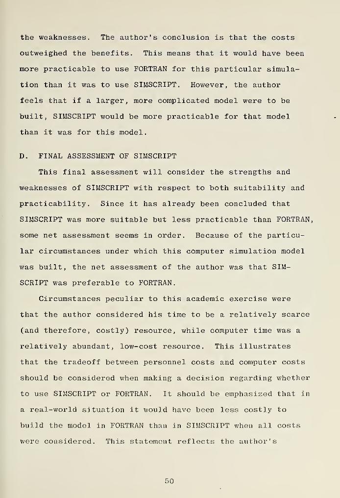
the weaknesses. The author's conclusion is that the costs

outweighed the benefits. This means that it would have been

more practicable to use FORTRAN for this particular simula-

tion than it was to use SIMSCRIPT. However, the author

feels that if a larger, more complicated model were to be

built, SIMSCRIPT would be more practicable for that model

than it was for this model.

D. FINAL ASSESSMENT OF SIMSCRIPT

This final assessment will consider the strengths and

weaknesses of SIMSCRIPT with respect to both suitability and

practicability. Since it has already been concluded that

SIMSCRIPT was more suitable but less practicable than FORTRAN,

some net assessment seems in order. Because of the particu-

lar circumstances under which this computer simulation model

was built, the net assessment of the author was that SIM-

SCRIPT was preferable to FORTRAN.

Circumstances peculiar to this academic exercise were

that the author considered his time to be a relatively scarce

(and therefore, costly) resource, while computer time was a

relatively abundant, low-cost resource. This illustrates

that the tradeoff between personnel costs and computer costs

should be considered when making a decision regarding whether

to use SIMSCRIPT or FORTRAN. It should be emphasized that in

a real -world situation it would have been less costly to

build the model in FORTRAN than in SIMSCRIPT when all costs

were considered. This statement reflects the author's

50

opinion that the use of SIMSCRIPT would not reduce program-

ming costs enough to offset the cost of the additional com-

puter time required.

51

V. SUMMARY AND CONCLUSION

A. METHODOLOGY FOR SIMULATING INTERNAL CONTROL

1. Success of Revised Methodology

The major conclusion of this thesis is that the re-

vised simulation methodology it presents can provide a more

efficient method of objectively evaluating internal control

than the original methodology used by Burns. The greater

efficiency of the revised methodology is due to the fact that

the error routines are more general in nature than the orig-

inal simulation program. Greater generality increases the

probability that the same error routines can be used to de-

fine other accounting and internal control systems.

The fact that the SIMSCRIPT program used to describe

the revised model required more computer time than a similar

FORTRAN program should not be used to argue that the revised

methodology is less efficient than the original methodology.

This is true because the revised methodology could almost as

easily have used FORTRAN. As was previously stated, the use

of SIMSCRIPT was completely independent of the use of the

revised methodology.

In addition, the argument that using FORTRAN to de-

scribe the revised model would be more costly than using

FORTRAN to describe the original model does not refute the

efficiency of the revised methodology. This is true because

the revised methodology is intended to reduce the cost of

describing internal control systems in addition to the one

52

dealt with in this thesis. The author admits that a high

set-up cost is incurred when programming the general purpose

error routines. However, once the error routines are writ-

ten, the cost which is incurred is that of arranging the

routines in the proper order and inserting the necessary

arguments into them. Consequently, the cost of preparing a

simulation model of an internal control system using the re-

vised methodology will be much less costly and much more

efficient once the general error routines have been written.

A concluding comment seems to be in order regarding

the significance of the output of an internal control system

simulation model prepared using the revised methodology.

This output would be represented by the mean and standard

deviation of the error present in the ending balance of each

account contained in the simulation model. These two statis-

tics provide an objective measure which can be used to de-

termine the adequacy of internal control in the system being

simulated. An assessment of adequacy can be made only after

the materiality of the error is determined when considering

the reported account balances of the real firm.

2 . Extension of Revised Methodology

Upon completion of the research performed as a basis

for this thesis, the author recognized one direction in

which this revised methodology could be extended. This ex-

tension related to the fact that the error processes in the

hypothetical firm were assumed to have discrete probability

distributions. Since real world error processes are likely

53

to be continuous, it might well be true that error processes

could be more easily represented by continuous probability

density functions. If this were the case, one of the argu-

ments for each general error routine would be the probabil-

ity density function of the error's magnitude. Such an

argument might possibly reduce the number of general error

routines that would be needed. At any rate, the author sug-

gests that further research should be conducted in the area

of developing error routines which are more general.

B. FEASIBILITY OF USING SIMSCRIPT

The use of SIMSCRIPT to describe the revised simulation

model provided the author with an opportunity to assess the

feasibility of using this language to describe simulation

models of internal control systems using the revised method-

ology. The conclusion which the author reached was that

SIMSCRIPT was more suitable than FORTRAN, but that SIMSCRIPT

required more computer time than FORTRAN. Thus the benefit

of requiring less programming time was offset against the

requiring of more computer time. The author feels that un-

less more complex simulation models are constructed, SIM-

SCRIPT would not need to be used. It is possible that some

other language (such as PL/I) might provide a less expensive

alternative than SIMSCRIPT. This is another area where fu-

ture research should be performed.

54

C. ISSUES TO BE RESOLVED

One of the purposes of this thesis was to identify the

basic requirements for a language which could be used spe-

cifically for the simulation of internal control systems.

Upon completion of this research, the author concluded that

several issues would have to be resolved before such basic

requirements could be identified. Unfortunately, resolution

of these issues required information the author could not

obtain, so it is possible only to state the issues which

must be resolved.

1. Optimal Size System to Simulate

One of the first issues which must be resolved deals

with the problem of deciding the optimal size internal con-

trol system to simulate. A good measure of size would be

the number of accounts contained in the system. For example,

the inventory accounting system dealt with in this thesis

was basically concerned with three inventory accounts. Two

additional accounts collected miscellaneous debits and cred-

its. An alternative system could have included all accounts

which were debited or credited in the miscellaneous accounts.

One such account would be accounts payable.

However, it might be more appropriate to simulate

the entire internal control system related to accounts pay-

able separately from the inventory accounting internal con-

trol system. Thus it can be seen that a decision must be

made regarding whether it is better to simulate each internal

55

control subsystem separately or to simulate the entire in-

ternal control system of a firm in one model.

Regardless of the decision which is reached, the

author has two suggestions which would simplify the simula-

tion process. First of all, the person designing the simu-

lation model should not concern himself with accounts whose

transactions are so few in number that subjective assessment

of the adequacy of internal control is feasible. Examples

of such accounts would be plant, property, and equipment,

owner's equity accounts, and long-term debt. Second, prep-

aration of a comprehensive chart of accounts would allow the

auditor to avoid having to set up each account involved in

the simulation. In addition, verifying a zero balance in

the accounts which were not involved would provide a control

to insure that all errors were recorded in the proper ac-

counts.

2. Conceptualization of Errors

Another issue which must be resolved deals with the

manner in which auditors conceptualize errors. An internal

control simulation language should be constructed in a man-

ner which would allow auditors to easily express error proc-

esses in the manner in which they conceptualize them. In

the model described in this thesis, all errors were concep-

tualized as either count (or quantity) errors or rate (or

price) errors. It might be true that auditors conceive the

monetary value of errors to be distributed according to the

normal distribution or some other statistical distribution.

56

On the other hand, they might consider the distribu-

tion of monetary errors detected during compliance tests to

represent a likely error probability density function. An-

other alternative might be that auditors think in terms

that could be expressed in the form of the beta distribution

used in PERT networks. If auditors construct optimistic,

most likely, and pessimistic error values, these estimates

could be used to determine the expected distribution of er-

ror.

Once it has been determined how auditors conceptual-

ize errors, routines could be written to simulate these

error processes. It should be pointed out that writing too

few routines might be more dangerous than writing too many.

Too few routines would cause auditors to discount the use-

fulness of simulation models, since they would have to fit

the real system into the model rather than fitting the model

to the real system. Too many routines would simply provide

an overly powerful (and thus, more expensive) language than

the auditor needs. Presumably there are a limited number of

ways in which errors are conceptualized by auditors, so any

routines which would not be used would simply add to the ex-

pense of performing simulations.

3 . Conceptualization of Controls

In a similar fashion, the manner in which controls

are conceptualized by auditors must be determined. Since the

author found programming the internal controls to be one of

the most difficult aspects of the simulation, he feels this

57

area needs more attention. In the model presented in this

thesis, the control itself could interject error into the

accounting system because of the manner in which it attempted

to correct previous errors. Thus it should be determined

whether auditors normally conceptualize controls as capable

of interjecting errors or whether they consider controls to

simply set the possible error equal to zero. A recent arti-

cle by Barry Cushing sheds some light on this subject by

presenting one method of conceptualizing the interaction of

controls and errors.

This issue is related to the conceptualization of

errors because it might be possible to reflect the effect of

controls in the error processes. This would be possible by

simply having the auditor express errors in terms of the er-

ror distribution which would be expected after the control

has been encountered. Unfortunately, it may not be possible

to do this in many of the more complex internal control sys-

tems.

Finally, it should be determined what criteria are

normally used to decide whether or not a given control will

be encountered. For example, the original model assumed

that the number of units by which production orders were

overstated determined whether or not an error was detected.

In other situations dollar values rather than unit quantities

12Cushing, B. E., "A Mathematical Approach to the Anal-

ysis and Design of Interna] Control Systems," The AccountingReview , v. XLIX, pp. 24-41, January 1974.

58

might be appropriate criteria. Whatever other criteria are

determined to be commonly found in internal control systems

should be provided for in an internal control simulation

language.

4. Structure of Input Data

The final issue which needs to be resolved deals with

how the input data should be structured in an internal con-

trol simulation language. In the model contained in this

thesis some data was specified in the main program (i.e.,

number of accounts, number of iterations, activity ceilings,

etc.), while some data was contained in the arguments used

when calling error routines. The author found that there

was a tradeoff between the number of arguments used in an

error routine and the number of error routines which were

necessary to describe all possible error processes. At the

limit, this meant that one error routine could have been

written to describe the entire system, but every variable in

the model would have to be an argument of this routine.

Since the author felt that the likelihood of an er-

ror in input data increased with the number of arguments, he

considered the use of only one error routine to be impracti-

cal. However, a viable alternative would be for the simula-

tion program to be designed so that only input data need be

prepared by the person describing the system. The simulation

program would then begin with a routine that would read in

the input data and check it to make certain that each vari-

able was given a value. If such a routine were included in

T.9

an internal control simulation language it could also gener-

ate error diagnostics regarding invalid or illogical input

data. The language might also include an option which would

allow the use of empirical data from the firm rather than

approximating such data by using random variate generators.

D. FINAL REMARKS

The author feels that once the issues stated above have

been resolved, it will be possible to determine the require-

ments for a language to be used for the simulation of inter-

nal control systems. Simulation models prepared with this

language would allow an auditor to supplement the traditional

subjective methods of assessing the adequacy of internal con-

trol with more objective methods. Since the superiority of

the simulation methodology over conventional auditing pro-

cedures has already been clearly demonstrated in Burns' dis-

sertation, the author feels that the time has come to develop

an internal control system simulation language.

60

APPENDIX A

OPERATIONAL FLOW CHART

OF REVISED SIMULATION MODEL

Establish routines and global variables

Specify the number of accounts to be simulated andthe number of iterations to be performed.

Dimension computer memory for all subscripted vari-ables .

At the beginning o f each iteration initialize accounterror balances to zero and establis h the seed valuefor generating raw material shipmen t and product ionorder quantities

.

For each raw mat.erial

,

set a count er equal to zeroand speci fy the ceilin g wh ich wi 11 control the numberof raw ma terial shipments to be ge nerated.

•'

I

Call routine QUANT1 to generate a value for the num-ber of units contained in a shipment.

Call routine ERR0R1 to generate a count error andprice error and determine if these errors shall oc-cur. If an error does occur, calculate its monetaryvalue •

Call routine ENTRY1 to record the value of the errorin the proper accounts.

Increment the counter by the number of unit s actuallycontained in the shipment . Test to determine if theceiling for raw material shipments has been exceeded.If the ceilin g has been exceeded, p:roceed t o the nextraw material. If the las t raw material has been simu-lated, procee d to the simulation of the productionprocess.

For each product, set a counter equal to zero andspecify the ceilings which will control the numberof units to be produced and the number of units to betransferred to finished goods.

Call routine QUANT1 to gener ate a value for the num-ber of units to be ind Lcat ed on a produc.tion or derin Departmen t I

62

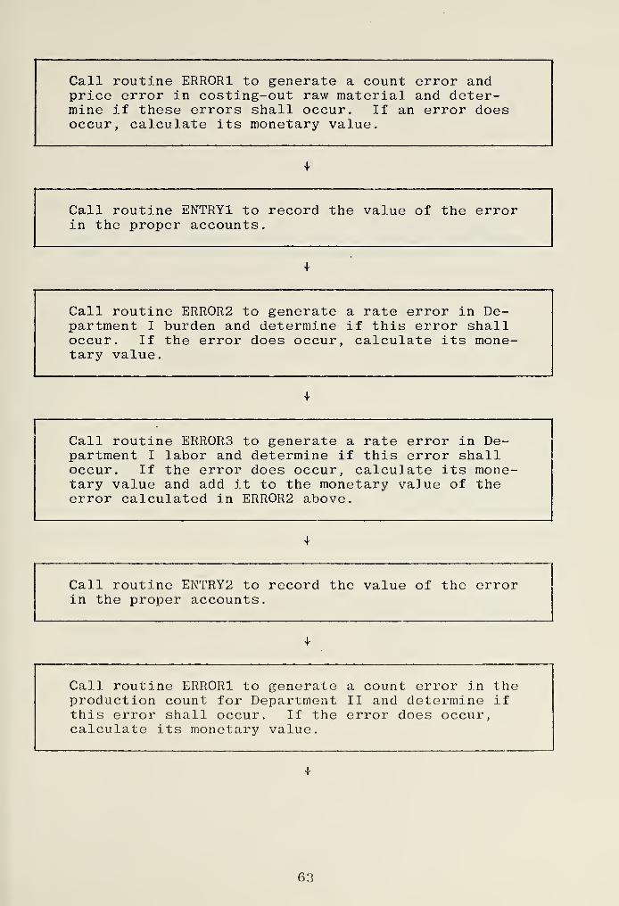
Call routine ERROR! to generate a count error andprice error in costing-out raw material and deter-mine if these errors shall occur. If an error doesoccur , calculate its monet iry value.


Call routine ERR0R2 to generate a rate error in De-partment I burden and det ermine if this error shalloccur. If the error does occur, calculate its mone-tary value

Call routine ERR0R3 to generate a rate error in De-partment I labor anc determine if this error shalloccur. If the error does occur, calcu late its mone-tary value and add i t to the monetary value of theerror calculated in ERR0R2 above.


Call routine ERR0R1 to generate a coun t error in theproduction count for Department II and det ermine ifthis error shall occur If the error does occurcalculate its monetary value

.

63

Call routine ERR0R2 to generate a rate error in De-partment II burden and determine if th is error shalloccur. If the error does occur, calcu late its mone-tary value.

Call routin e ERR0R3 to generate a rate error in De-partment II labor and determine if this error shalloccur. If the error does occur, calcu late its mone-tary value and add i t to the monetary value of theerror calcu lated in ERR0R2 above


Determine if the ceiling for number of units to betransferred to finished goods has been exceeded.If this ceiling has been exceeded, do not transferthese unit s to finished goods , but do continue simu-lating the production process

If th e ceiling for the number of units to be trans-ferre d to finished goods has not been exceeded, simu-late the control p erformed by the weig h-count opera-tor. This control will detect an overstatement ofthe count on a pro duction order i f its magnitude isgreat er than twent y units.

64

If the control detect s an overstatement in the pro-duction count, it corrects the count on the produc-tion order and sends the production order t o theaccount ing department . If no overstatement is de-tected, no correction is made when the productionorder is forwarded.

Simulate the operations performed in the accountingdepartment. This is done by calling the routineERR0R1 to gen erate a pricing error and determine ifthis error is to occur. If the error does occur,calculate its monetary value


Simulate the corrections made by the accounting de-partment if the control detected an overstatement.This is done by calculating the iidjus tments neces-sary to correct the errors which were assumed to bepresent in the .raw materials and work-in-process ac-counts

.

The monetary value of these errors is cal-culated and rou tine ENTRY3 is ca Lied to record thevalue of the error in the proper accounts

.

Increment the counter by the number of units statedon the production order. Test to determine if theceiling for number of units to be produced has beenexceeded. If the ceiling has been exceeded, proceedto the next product. If the last product has beensimulated, proceed to the section of the programwhich prints the output.

65

Print out the ending account bal ance, which containsthe monet ary va Lue of the error in the ending accountbalance. After this has been do ne for each account,store the value in an array for later processing.

Determine if the required number of iterations havebeen performed. If they have not all been performed,proceed to the beginning of the program.

If the required number of iterations have been per-formed, calculate the mean and standard deviationof the error in the account balances which were storedearlier Upon calculation of these statistics

,

printthem out.

66

//SIMRUNS2 JCB ( 247 1 , 0234, 6418) ,' C. M. PCN • ,TI ME= ( 14, 30

)

// EXEC SIM25CLG, REGION. GO=100K//SIM.SYSIN 00 *

PREAMBLENORMALLY MODE IS REALDEFINE INITIAL. QUANTITY AS AN INTEGER VARIABLEDEFINE ERROR AS A REAL VARIABLEDEFINE ACCOUNT AS A REAL 1-D I MENS IONAL ARRAYDEFINE ACCT. TITLE AS AN ALPHA 1-DI MENSIONAL ARRAYDEFINE SAMPLE AS A REAL 2-DI MENS I ONAL ARRAYDEFINE NO. OF. ITERATIONS AS AN INTEGER VARIABLEDEFINE ERR0R1 AS A ROUTINE WITH 5 ARGUMENTSDEFINE QUANT1 AS A ROUTINE WITH 3 ARGUMENTSDEFINE ENTRY1 AS A ROUTINE WITH 2 ARGUMENTSDEFINE COUNTER AND QUOTA AS INTEGER VARIABLESDEFINE NUMBER. OF.ACCOUNTS AS AN INTEGER VARIABLEDEFINE ENTRY2 AS A ROUTINE WITH 2 ARGUMENTSDEFINE ENTRY3 AS A ROUTINE WITH 2 ARGUMENTSDEFINE ERR0R2 AS A ROUTINE WITH 6 ARGUMENTSDEFINE ERR0R3 AS A ROUTINE WITH 5 ARGUMENTSDEFINE COUNT. ERROR AS AN INTEGER VARIABLEDEFINE HOURS AND RIGHT. HOURS AS REAL VARIABLESDEFINE TOTAL. COUNT. ERROR AS AN INTEGER VARIABLEDEFINE QU0TA1 ANO QU0TA2 AS INTEGER VARIABLESLAST COLUMN IS 60END

MAINLET NUMBER. OF. ACCOUNTS = 6LET NO. OF. ITERATIONS = 100RESERVE SAMPLE AS NUMBER .OF . ACCOUNTS BY NO .OF

.

ITERATIONSRESERVE ACCOUNT AND ACCT. TITLE AS NUMBER. OF .ACCOUNTSFOR J = 1 TO NO. OF. ITERATIONS DO "BEGIN MAIN"FOR I = 1 TO NUMBER. OF. ACCOUNTS DO LET ACCOUNTd,) = 0.0 LOOPLET SEED.V12) = 663743814LET ACCT.TITLE(l) = "MISC. DEBIT"LET ACCT.TITLE(2) = "RAW MATERIAL"LET ACCT.TITLE(3) = "WORK IN PROCESS"LET ACCT.T1TLE<4) = "FINISHED GOODS" " ' "

LET ACCT.TITLE15) = "MISC. CREDIT"LET ACCT.TITLE(6J = "COMBINED INVENTGRY"LET COUNTER = "RAW MATERIAL 1"LET QUOTA = 40000• BEGIN!'CALL QUANT1 (200.0,25.0,2)CALL ERRORK . 25 ,-. 10, . 10, 13. 50,6 . 50)CALL ENTRY1(2,5)LET COUNTER = COUNTER + INITI AL. QUANT ITYIF COUNTER < QUOTA GO TO 6EGIN1ELSELET COUNTER = "RAW MATERIAL 2"LET QUOTA = 34000•BEGIN2"CALL QUANTK180. 0,30. 0,2)CALL ERRORK .25, -.10, .10,16.70,8.00)CALL ENTRY1(2,5JLET COUNTER = COUNTER + INI TIAL. QUANTITYIF COUNTER < QUOTA GO TO BEGIN2ELSELET COUNTER = "RAW MATERIAL 3"LET CUOTA = 34000•BEGIN3'CALL QUANTK 200.0,25.0,2)CALL ERRORK .25,-. 10,. 10 ,6. 50, 13. 50

J

CALL ENTRY1(2,5)LET COUNTER = COUNTER + INI T I AL . QUANT I TYIF CCUNTtR < QUOTA GO TO BEGIN3ELSELET COUNTER = "RAW MATERIAL 4"

07

LET QUOTA = 32000•BEGIN4'CALL QUANTK 180.0,30.0,2)CALL ERRORK . 25 ,-. 10, . 10, 8. 00, 16. 70)CALL ENTRY1(2,5/LET COUNTER = COUNTER + INI T I AL. QUANT ITYIF CGUNTER < QUOTA GO TO BEGINSELSELET COUNTER = "PRODUCT 1"LET GUQTA1 = 33600LET CU0TA2 = 30280•BEGIN. PI*CALL QUANTK 150.0,35.0,2) "DEPT. 1 PRODUCTION"CALL ERRCRK .15, . 10, . 10, 13. 50,6.50) "DEPT. 1 DIR. MATL."CALL ENTRYK3,2)CALL ERR0R2(.O3, .06, .04, .03,12.35,11.40) "DEPT. 1 BURDEN"CALL ERROR3(.10,6.00,5.60, .50,6.20) "OEPT. 1 DIR. LABOR"CALL ENTRY2(3,5)CALL ERRORK .03, .05,0.0,0.0,0.0) "DEPT. 2 PRODUCTION"LET INITIAL. QUANTITY = I NIT I AL. QUANT ITY - TOT AL . COUNT . ERRORLET TOTAL. COUNT. -ERROR = TOTAL. COUftT . ERROR + COUNT. ERRORLET COUNT. ERROR = TOT AL . COUNT .ERRORCALL ERR0R2( . 08 , .04 , . 04 , . 08 , 51.55 , 44. 05 ) "DEPT. 2 BURDEN"CALL ERRCR3(. 10, 5.40, 6 . 20 ,. 50, 5 . 60) "DEPT. 2 DIR. LABOR"CALL ENTRY3(3,5)IF COUNTER >= QU0TA2 AND COUNTER < QUOTA!

GO TO TEST. PIELSEIF TOTAL. COUNT. ERROR > 20 "THE CHECK DETECTS AN ERROR"LET COUNT. ERROR =CALL ERRORK -1.0, 0.0,. OS, 16. 929, 9. 19)CALL ENTRY3(4,3)LET ERROR = T OTAL. COUNT . ER"ROR * 3.429CALL ENTRY3(1,3)LET ERROR = TOTAL. COUNT . ERROR * 13.50CALL ENTRY3(2,3)GO TO TEST. PI "END OF ERROR CORRECTION"ELSECALL ERRORK -1.0,0.0,. 08, 16. 929, 9. 19)CALL ENTRY3(4-,3)"•TEST. PI'LET COUNTER = COUNTER + INI TIAL. QUANT ITYIF^CCUNTER < QU0TA1 GO TO BEG4N.P1

LET COUNTER ^ "PRODUCT 2"LET GU0TA1 = 33000LET QU0TA2 = 309S4f BEGIN. P2'CALL CUANTK150. 0,35. 0,2) "DEPT. 1 PRODUCTION"CALL ERRORK .15, .10, .10, 16. 70,3.00) "DEPT. 1 DIR. MATL."CALL ENTRYi(3j2)CALL ERRCR2( .08, .09, .06, .08, 12.85,11.40) "DEPT. 1 BURDEN"CALL ERR0R3( .10, 6.00,5.o0, .50, 6. 20) "DEPT. 1 DIR. LABOR"CALL ENTPY2(3,5)CALL ERRORK .03, .05,0.0,0.0,0.0) "DEPT. 2 PRODUCTION"LET INI 1 IAL. QUANTITY = I NI T I AL. QUANT i TY - TOTAL. COUNT. ERRORLET TOTAL.COUNT- ERROR = TOT AL .COUNT . ERROR + COUNT. ERRORLET COUNT. ERROR = TOTAL . COUNT . ERRORCALL ERRCR2( .08, .09, .06, .08,51.55,44.05) "DEPT. 2 BURDEN'*CALL ERR0R3< .10,5.40,0. 20, .50,5.60) ''DEPT. 2 DIR. LABOR"CALL ENTRY313.5)IF COUNTER >= QUQTA2 AND COUNTER < QU0TA1

GO TO TEST.P2ELSEIF TOTAL. COUNT. ERROR > 20 ''THE CHECK DETECTS AN ERROR"LET COUNT. ERROR =CALL ERRORK -1.0, 0.0, .08,21.8435,12.5315)CALL ENTRY3U.3)LET ERROR = f 07 AL. COUNT . ERROR * 5.1435CALL ENTRY3(1,3)LET ERROR = T OTAL. COUNT . ERROR * 16.70CALL ENTRY3(2,3)

68

GO TO TEST.P2 "END OF ERROR CORRECTION"ELSECALL ERROR1 (-1.0,0.0, .08,21.8435,12.5315)CALL ENTRY3l4,3)•TEST.P2*LET COUNTER = COUNTER + INITI AL . QUANT I TYIF COUNTER < QU0TA1 GO TO BEGIN. P2ELSELET COUNTER = " PRODUCT 3"LET CU0TA1 = 33000LET CU0TA2 = 29777•BEGIN. P3'CALL QUANTK 150.0,35.0,2) "DEPT. 1 PRODUCTION"CALL ERRORK .15, . 10, . 10 , 6.50, 13 . 50) "DEPT. 1 DIR. MaTL."CALL ENTRYK3.2)CALL ERRQR2( .08, .04, .06, .03, 11.40,12. 85) "DEPT. 1 BURDEN"CALL ERR0R3( . 10, 6 .00, 5 . 60, . 50,6 . 20 ) "DEPT. 1 DIR. LABOR"CALL- ENTRY 2 13, 5)CALL ERRORK .08, .05,0.0,0.0,0.0) "DEPT. 2 PRODUCTION"LET INITIAL. QUANTITY = I NIT I AL . QUANT IT Y - TOTAL. COUNT . ERRORLET TOTAL. COUNT. ERROR -= TOTAL.COUNT. ERROR + COUNT. ERRORLET COUNT. ERROR = TOTAL . COUNT . ERRORCALL ERR0R2(.08,.04,.06,.08,44.05,51.55) "DEPT. 2 BURDEN"CALL ERR0R3(.10,5^4O,6.20,.50,5.60) "DEPT. 2 DIR. LABOR"CALL ENTRY3<3,5)IF COUNTER >= QU0TA2 A1MD COUNTER < QU0TA1

GO TO TEST.P3ELSEIF TOTAL. COUNT. ERROR > 20 "THE CHECK DETECTS AN ERROR"LET COUNT. ERROR =CALL ERROR! (-1.0, 0.0,. 03, 9. 19, 16. 929)CALL £NTRY3(4,3)LET ERRUK = TOTAL. COUNT. ERROR * 2.-69CALL ENTRY3(1,3)LET ERROR = TOTAL. COUNT . ERROR * 6.50CALL ENTRY3{2,3)CO TO TEST.P3 "END OF ERROR CORRECTION"ELSECALL ERRORK -1.0, 0.0,. 08, 9. 19, 16. 929)CALL ENTRY3(4,3)•TEST.P3*LET COUNTER = COUNTER + INI TI AL. QUANT I TY «.

IF COUNTER < QU0TA1 GO TO BEGIN. P3ELSELET COUNTER = "PRODUCT 4"LET CU0TA1 = 28900LET CUQTA2 = 21719•BEGIN. P4«CALL QUANTK150. 0,35. 0,2) "DEPT. 1 PRODUCTION"CALL ERRORK .15, .10, .10, 8. 00, 16. 70) "DEPT. 1 DIR. MATL."CALL ENTRY1(3,2)CALL ERR0R2(. 08, .06, .09, .08,11.40,12.85) "DEPT. 1 BURDEN"CALL ERROR3(.10,6.00,5.60,.50,6.20) ''DEPT. 1 DIR. LABOR"CALL ENTRY2(3,5)CALL ERRORK .08, .05,0.0,0.0,0.0) "DEPT. 2 PRODUCTION"LET INITIAL. QUANTITY = I NI T I AL . QUANT I TY - TOT AL . CCUNT . ERRORLET TOTAL. COUNT. ERROR = TOTAL .COUNT . ERROR + COUNT. ERRORLET COUNT. ERROR = TOTAL. COUNT . ERRORCALL ERR0R2( .08, .06, .09 , .08, 44. 05 ,51 . 55) "DEPT. 2 BURDEN"CALL ERRORK . 10, 5.40, 6.20, .50,5.60) "DEPT. 2 DIR. LABOR"CALL ENTRY3(3,5)IF COUNTER >= QU0TA2 AND COUNTER < QU0TA1

GO TO TEST.P4ELSEIF TOTAL. COUNT. ERROR > 20 "THE CHECK DETECTS AN ERROR"LET CCUNT. ERROR =CALL ERRORK- 1. 0,0.0,. 08, 12. 5315, 21. 8435)CALL ENTRY3(4,3)LET ERROR = TOT AL. COUNT . ERROR * 4.5315CALL ENTRY31 1,3)LET ERROR = T OTAL. COUNT . ERROR * 8.00CALL ENTRY3(2,3)

69

GO TC TEST.P4 "END OF ERROR CORRECTION"ELSECALL ERRORK- 1.0, 0.0,. OS, 12. 53 15, 21. 8 435)CALL ENTRY3(4,3)' TE ST. P4

'

LET COUNTER = COUNTER + INIT I AL .QUANT I TYIF COUNTER < QU0TA1 GO TO BEGIN. P4ELSE•OUTPUT' "USER NEEO NOT SPECIFY THIS"LET ACC0UNT(6) = ACCCUNT(2) + ACCGUNT(3) + ACC0UNT(4)FOR I = 1 TO NUMBER. OF. ACCOUNTS DOPRINT 1 LINE WITH ACCT .

T

ITLE ( I ) AND ACCOUNT(I) THUS

LQCPSKIP i OUTPUT LINE

FOR I = 1 TO NUMBER. OF. ACCOUNTS DOLET SAMPLE(I,J) = ACCOUNT(I)LOOP

LOOP • 'END MAIN"FOR I = 1 TO NUMBER. OF. ACCOUNTS DO

FOR J = 1 TO NO. OF. ITERATIONS DOCOMPUTE XBAR AS THE MEAN AND SIGMA AS THE STD.DEV OF .

SAMPLE ( I, J)LOOP

PRINT i LINE WITH ACCT .T ITLE ( I J , XBAR, AND SIGMA THUS*^ -J- -.v* %-v %A* -J, -*3s -J* -v ^s -*- ^' *i^ i&* *'* *J~ *J* *** ^- Vr "^^ V' -J* V' ^^ *"-* *-** **'-' ^' *V *J* *-'" *** * 1-'

-,- .,< *y- *~ -,- -p -i- -v- ^ n, -,- ^- -,» J,- -^ -,- *r -i* "V -v -** -*r *r # <v -v »r TV*, «r ,«'"t* s n"p

LCCPEND

ROUTINE QUANT 1( MEAN, STD.DEV, STREAM)LET INITIAL. QUANTITY = NORMAL .F { MEAN , STD . DEV, STREAM

)

LET TOTAL. COUNT. ERROR =END

ROUTINE ERROR 1< PROB. OF. COUNT. ERROR, COUNT. ERROR. PERCENT,PR Ctf. CF. PRICE. ERROR, CORRECT. PR I CE, WRONG. PR ICE)

NORMALLY MODE IS REALIF PROB. OF. COUNT. ERROR < 0.0LET Rl = PROB. OF. COUNT. ERROR - 1.0GO TC NEXT1 "COUNT ERROR ALREADY HAS A VALUE"

ELSELET Rl = RANDOM. F(3)IF Rl < PROB. OF. COUNT. ERROR

LET COUNT. ERROR = INIT I AL . QUANT ITY * COUNT . ERROR. PERCENTGO TO NEXT!

ELSE LET COUNT. ERROR ='NEXT1' ,

LET R2 = RANDOM. F(4)IF R2 < PROB. OF..PRICE. ERROR

LET PRICE. ERROR = WRONG. PRICE - CORRECT. PR I C

E

GO TO NEXT

2

ELSE LET PRICE. ERROR = 0.0•NEXT2*IF Rl < PROB. OF. COUNT. ERROR OR R2 < PROB. OF. PR ICE . ERROR

LET ERROR = (COUNT. ERROR * CORR ECT . PP. I CE )

+ (PRICE. ERROR * ( IN I

T

IAL . QUANT 1 TY + COUNT. ERROR)

J

GO TO 'NEXT 3*ELSE LtT ERROR = 0.0•NEXT3'END

ROUTINE ERROR 2 (PROB. HRS. ERROR, RIGHT. DIR. LABOR. HRS,WRONG .DIR .L ABOR. HRS , P ROB . R AT E . E RRO R , CORR EC T . R AT E

,

WRONG. RATE)LET R2 = RANDOM. F( 5)IF P2 < PROB. HRS. ERROR

LET HOURS = WRONG. DIR. LABOR. HRSGO TO NEXT1

ELSE LET HuUkS = RIGHT . DI R. LABOR. HRS

70

•NEXT1*LET R3 = RANDOM. F(6)IF R3 < PROB. RATE. ERROR

LET RATE = WRONG. RATEGO TO NEXT2

ELSE LET RATE = CORRECT. RATE'NEXT2*LET ERRCR = ERROR +• (COUNT. ERROR * HOURS * RATE)LET RATE. ERROR = (( INITIAL . QUANTITY + COUNT. ERROR)

* ((HOURS * RATE) - ( R IGHT .DI R . LABOR . HRS * CORRECT. RATE ))

)

LET ERROR = ERROR + RATE. ERRORLET RIGHT.HOURS = RIGHT .DIR. LABOR .HRSEND

ROUTINE ERR0R3 ( PROB. OF. RATE. ERROR, WRONG. RATE. ltWRCNG. RATE. 2,PRCB. OF. WRONG. RAT E.l, CORRECT. RATE)

•NORMALLY MODE IS REALLET R3 = RANDOM. F(7)IF R3 < PROB. OF. RATE. ERROR

LET RATE = WRONG. RATE.

2

GO TO TEST1ELSE LET RATE = CORRECT. RATEGO TC FINISH«TEST1«LET R4 = RANDOM. F( 8)IF R4 < PROB. OF. WRONG. RATE.

1

LET RATE = WRONG. RATE.

1

ELSE•FINISH'LET ERROR = ERROR + (COUNT. ERROR * HOURS * RATE)LET RATE. ERROR = ( I NIT I AL .QUANTI T Y + COUNT. ERROR)

* ((HOURS * RATE) - ( R I GHT . HOURS * CORRECT. RAT E ) )

LET ERROR = ERROR *• RATE. ERROREND

ROUTINE ENTRYK CEBIT, CREDIT)NORMALLY MODE IS INTEGERLET ACCOUNT (DEBIT) = ACCOUNT ( DEBI T) + FRRCRLET ACCCUNT(CREDIT) = ACCOUNT ( CREDIT ) - ERRORLET ERRCR = 0.0LET TOTAL. COUNT. ERROR =END

ROUTINE ENTRY2( CEBIT, CREDIT)NORMALLY MODE IS INTEGER-LET ACCCUNT(DEBIT) = ACCOUNT (DEB I T) + ERRORLET ACCOUNT (CREDIT) = ACCOUNT (CREDIT ) - ERRORLET INITIAL. QUANTITY = INIT I AL. QUANTITY + COUNT. ERRORLET TOTAL. COUNT. ERROR = TOTAL. COUNT

.

ERROR + COUNT. ERRORLET ERROR = 0.0END

ROUTINE ENTRY3( CEBIT, CREDIT)NORMALLY MODE IS INTEGERLET ACCCUNT(DEBIT) = ACCOUNT

(

DEB I T ) + ERRORLET ACCCUNT(CREDIT) = ACCOUNT (CREDIT ) - ERRORLET ERRCR = 0.0END

71

LIST OF REFERENCES

Burns, D. C. , Audit Evidence Evaluation Using ComputerSimulation with Special Emphasis on Ascertaining theReliability of Accounting Data , Doctoral Dissertation,Indiana University, Bloomington, Graduate School ofBusiness, 1971.

Committee on Auditing Procedure, Statement on AuditingStandards No. 1 , American Institute of Certified PublicAccountants, Inc., 1973.

Cushing, B. E., "A Mathematical Approach to the Analysisand Design of Internal Control Systems," The Account-ing Review , v. XLIX, January 1974.

Emshoff, J. R. and Sisson, R. L. , Design and Use of Com-puter Simulation Models , Macmillan, 1970.

Fishman, G. S., Concepts and Methods in Discrete EventDigital Simulation , Wiley, 1973.

Kiviat , P. J., Villanueva, R. , and Markowitz, H. M.

,

SIMSCRIPT II . 5 Programming Language, p. v, Consolidated

Analysis Centers, Inc., 1973.

Naval Postgraduate School Report 55Bu73111A, A ComputerSimulation Case for the Auditing Classroom , by D. C.Burns, November 1973.

72

INITIAL DISTRIBUTION LIST

No. Copies

1. Defense Documentation Center 2Cameron StationAlexandria, Virginia 22314

2. Library, Code 0212 2Naval Postgraduate SchoolMonterey, California 93940

3. Department Chairman, Code 55 1

Department of Operations Research andAdministrative Sciences


4. Asst. Professor David C. Burns, Code 55Bu 1

Department of Operations Research andAdministrative Sciences


5. ENS Gerald G. Brown, USNR, Code 55Zr 1Department of Operations Research and

Administrative SciencesNaval Postgraduate SchoolMonterey, California 93940

6. LTJG Carl Maynard Pon , USNR 1

1245 Leahy RoadMonterey, California 93940

73

~- 153120ThesisP73H5 Pon

^ metho(jology for the ^simulation of internal

,

control systems.

I 9 hay li

i HioThesis

P7345 Ponc '-^ A methodoloav for the

simulation of internalcontrol systems.

20

TSS^mi^SSSSSm

IIIIIIWW"™™"3 2768 001 92318 8

DUDLEY KNOX LIBRARY

a methodology for the simulation of internal control systems

Documents