a methodology for randomly selecting ...frawley, william e. 1 a methodology for randomly selecting...

Frawley, William E. 1

A METHODOLOGY FOR

RANDOMLY SELECTING TRAFFIC COUNT LOCATIONS

IN TEXAS – RESULTS AND BENEFITS

William E. Frawley Texas Transportation Institute

110 N. Davis Dr., Ste 101 Arlington, TX 76013 Phone: 817.462.0599

Fax: 817.461.1239 E-mail: [email protected]


ABSTRACT

The Texas Department of Transportation (TxDOT) identified the need for a more accurate estimation of vehicle miles traveled (VMT) on streets functionally classified as local. The Texas Transportation Institute (TTI) developed a procedure to randomly select traffic count sites on local streets that results in a statistically valid estimation of local street VMT. This procedure has evolved from using grids overlaid on hard copy maps to a mostly electronic process. In either scenario, grids are overlaid TxDOT maps that include all streets in a given area. All grid cells are assigned sequential numbers and then a relative range of random numbers is generated. The person performing the process then locates the grid cells that correspond to the randomly selected numbers in the order in which they were generated. Each time a cell is selected that contains a local street, a traffic count site is added to the map. This process is repeated until an appropriate number of sites have been selected. Statistical analyses have determined how many count locations are necessary in order to provide a representative sample of traffic counts in areas, depending on the population. Median values of counts identified the number of counts at which the diminishing rate of return on the investment in the counts occurs. This procedure has resulted in median traffic count volumes on local streets that more realistically represent the variety of local streets that exist. These median volumes, derived from randomly selected sites, are considerably lower than the median volumes derived from historical count locations that are not randomly selected. In addition, the use of randomly selected traffic count locations has made it possible for TxDOT to reduce by thousands the number of counts it performs across the state.


BACKGROUND There are currently four metropolitan areas in Texas classified as air quality non-attainment areas – Houston, Dallas-Fort Worth, El Paso, and Beaumont-Port Arthur. One factor used to determine if non-attainment areas are making progress toward improving air quality is the estimation of vehicle miles traveled (VMT) on streets functionally classified as “local.” These estimations are based on 24-hour traffic counts taken on local streets. While the Texas Department of Transportation (TxDOT) uses the federally approved functional classification system, occasionally a metropolitan area may have a slightly different functional classification system used for modeling purposes. Some areas have more than one local street VMT estimate, depending on which functional classification system and other methodology steps were used.

TxDOT approached the local street VMT issue through the Technical Working Group on Air Quality (TWG). The TWG is comprised of representatives from various agencies, including metropolitan planning organizations (MPOs), cities, the Environmental Protection Administration (EPA), the Texas Natural Resource Conservation Commission (TNRCC), Federal Highway Administration (FHWA), and TxDOT. The process described in this document has been reviewed by TWG members and is considered to be part of the interagency consultation process identified in EPA’s Final Rule (40 CFR Part 93.105) on Transportation Conformity.

TxDOT, as well as the affected metropolitan areas, needs one consistent, precise process for estimating local street VMT. It is vital that the process be usable in any given metropolitan area. The Texas Transportation Institute (TTI) project team working on this task, through an interagency agreement with the Traffic Section of the Transportation Planning and Programming Division (TPP(T)), has developed a methodology to count traffic on local streets and use the results to estimate local VMT.

Local Street Definition Local streets are those that are not included in any of the other functional classifications in rural or urban areas, according to the FHWA publication “Highway Functional Classification, Concepts, Criteria, and Procedures.” These definitions also state that the primary purposes of local streets are to provide access to adjacent properties over relatively shorter routes with limited through traffic. The publication also indicates that local streets should generally comprise approximately 65-80 percent of the total roadway system and contain 5-20 percent of total VMT in rural areas and 10-30 percent of total VMT in urban areas (1).

TxDOT Saturation Count Processes TxDOT operates two simultaneous traffic count processes – the annual counts and the saturation counts. TxDOT performs annual counts at virtually the same locations every year in each of the 25 districts. These counts are used to develop traffic volume trends and other annual reporting information.

In any given year TxDOT also performs saturation counts in approximately five districts throughout the state. The saturation count process involves counting traffic volumes at thousands of locations within each metropolitan area, multitudes more than are performed during the annual count process. The saturation counts on streets other than local functional classification, are primarily used for traffic model development in the metropolitan areas. Therefore, the count locations involved have been established for modeling purposes rather than for creating statistically valid default traffic volumes.


Field Counting Procedures The saturation counts, as well as the randomly selected counts that are simultaneously performed, are 24-hour tube counts. Counts are typically performed during months in which school is in session. The Dallas-Fort Worth counts included in this document, however, were performed in the summer months, since that is when TxDOT had scheduled the area’s annual counts. This was the only opportunity during the calendar year to collect randomly selected counts in the Dallas-Fort Worth area. Saturation counts will next be conducted in the Dallas-Fort Worth area in 2004. Contracted crews perform the counts for TxDOT according to schedules created by the Traffic Section’s Technical Services staff. The contracted crews collect the data and submit them to TxDOT for analysis and reporting.

When applicable, all counts conducted and analyses performed through this process are completed in conformity with the 2001 Traffic Monitoring Guide.

APPROACH TO PROBLEM For obvious reasons TxDOT cannot possibly count traffic on every local street in any metropolitan area. Therefore, it is necessary to collect traffic count samples at a variety of locations. The questions that initially arose during the development of this process were: 1) how many samples to collect in a given area, and 2) where to locate the traffic count station locations.

Regarding the first question, the project team decided, for statistical purposes, to choose traffic count locations using a random selection process. This decision led to the next question of how to specifically select the station locations. The selection process should introduce no undue bias into the methodology, giving as many local streets as possible a chance to be selected. At the same time the selection process cannot be too cumbersome to implement effectively.

The issue of selecting count locations is dependent on the solution to the issue of how many samples to collect. Once it was decided to use a random site selection process, with as little bias as possible, the project team realized that it would have little if any choice in where specific counts would be located. This meant that human decision could not determine how count station locations were to be distributed geographically in any given area.

MANUAL RANDOM COUNT SITE SELECTION PROCESS The process for randomly selecting count locations has evolved from a manual process to a primarily electronic process. This section describes the original manual process and the following section describes the newly implemented electronic process.

Grids

The project team developed a process for randomly selecting traffic count station locations. This process overlaid a grid on top of TxDOT’s station location maps and/or functional classification maps for an area and assigned a number to each grid cell. The grid cells typically contain segments of only a few streets, but are large enough to easily work with. A unique identification number is assigned to each grid cell, beginning with “1” and continuing through the number of cells being used. Grouped in sets of 100, each set of cells is divided by bold borders. The actual


numbering works in a matrix system, with the “ones units” going across the top of the grid and the “tens units” going down the edge of the grid. Figure 1 provides an example of a grid overlay. For counties within air quality non-attainment areas, the grids are overlaid on the entire county, capturing large urban, small urban, and rural areas together.

Random Numbers Team members used Microsoft Excel to generate random numbers in a range equal to the number of cells on the grid. The team selected more than twice as many random numbers as the number of station locations that were to be selected. This was necessary because some of the grids (once overlaid on the maps) contained no streets. This situation varied depending on the amount of undeveloped land on a given map. In addition, a random number was sometimes repeated in the Excel output, which would bring the actor back to a cell previously selected. No more than one street was selected from an individual cell.

Maps This methodology uses two types of maps – roadway functional classification and traffic count station location (Figure 2). Functional classification maps verify that randomly selected count locations are on local streets. There are two variations of functional classification maps – urban and rural. TxDOT district offices provide the urban functional classification maps, used to verify functional classifications in small urban areas (with populations between 5,000 and 49,999, inclusive). TPP(T) provides the rural functional classification maps, showing functional classifications for roads in rural areas (populations of less than 5,000).

When possible, the project team selected random count locations on functional classification maps in order to immediately verify functional classifications of selected roads. In some cases, the team transferred functional classification information from functional classification maps to station location maps to efficiently select random count locations and immediately verify functional classifications.

After randomly selecting counts on functional classification maps, the TTI team transferred the count identification numbers to station location maps. This step minimized the scheduling efforts performed by Traffic Section’s Technical Services staff.

Station Location Selection The station location selection process began by finding the grid cell corresponding to the first random number generated. If that cell contained at least one street, the street closest to the center of the grid was selected for the station location. If the cell contained no streets, the next random number was used to repeat the process. This process continued until the desired number of count station locations had been selected.

The only variation to the count site selection methodology was in the Lubbock urbanized area. When selecting counts in Lubbock, the project team used two more selection processes in addition to the grid method. One process randomly selected names of local streets from a list. A count station location was placed on the streets selected. While the project team selected the street names randomly, there was some bias in deciding exactly where to place the count station on the street.


The other method tested in Lubbock distributed the count station locations evenly throughout the urbanized area. Streets for these sites were selected by geographic location (to get an equal spread throughout the area) as well as by length of streets (to get an equal distribution among short, medium-length, and long streets. This selection process was greatly biased because humans completely determined where to place the count station locations. The project team is analyzing these data sets and will have results in the near future.

ELECTRONIC RANDOM COUNT SITE SELECTION PROCESS TxDOT and TTI have developed an electronic process through which counts can be randomly selected with minimal use of hard copy maps. An electronic grid is prepared and overlaid on top of an electronic map as a layer. This grid can be customized to only cover streets, eliminating the occurrence of grid cells being placed over empty land without streets as occurred through the manual process. Each of the cells receives unique identifying numbers and a corresponding random number list is generated. The person performing the selection process then types in each number from the list (one at a time) and the appropriate cell is highlighted automatically. The person can then compare the electronic map on the computer screen with a hard copy functional classification map to determine if a street functionally classified as local is in the cell. When the functional classification update process is complete in the near future, the functional classification maps will be electronic also and eliminate the need for the hard copy map comparisons.

RANDOM COUNT DATA ANALYSIS After contracted crews perform the traffic counts and provide the raw data to TxDOT, the Technical Services staff sends the randomly selected counts to TTI. TxDOT does not analyze or apply any adjustment factors to these data prior to sending them to TTI, who performs its own analysis using steps described in this section.

Functional Classification Verification Throughout the entire random count site selection process, the project team routinely performed spot checks of functional classification for the selected sites, regardless of count volumes. Staff also verified functional classifications for count locations that had volumes over 10,000 vehicles, since such volumes are definitely uncharacteristic of streets truly serving local purposes. No data from streets functionally classified as local was thrown out of the data set. Functional classifications for some of these locations in various areas were actually local, while some classifications were corrected before subsequent analysis steps were performed.

In the case of Houston, however, all randomly selected sites were verified. This level of verification was performed for its potential use in air quality conformity analysis, and due to the complicated nature of the Houston area counts, which included a combination of urban and rural areas crossing county lines throughout the district.

Duplicate Counts Through the random count location selection process, occasional sites are selected at the same locations as historical TxDOT count station locations. To save resources and maintain the most


efficient count process possible, only one count is typically performed at the location. This provision does add an extra step to TTI’s analysis, though, since duplicate historical count station locations must be identified and the count data transferred to TTI’s count database.

Statistical Analysis A TTI statistician analyzed the traffic count data from the randomly selected sites and the data from TxDOT’s historical count station locations, except in the case of Dallas-Fort Worth, since no saturation counts were performed simultaneously with the randomly selected counts. The counts were analyzed statistically in the order in which they were selected to maintain the integrity of the random selection process. This analysis is based on the median values of sample sizes (described in the next subsection) and resulted in recommended sample sizes for different sized urban areas.

Mean v. Median The median is defined as the number in which 50% of the data are less than or equal to the number and 50% of the data are greater than or equal to the number. It is the center data point when all the data are arranged in a line. Averages are defined as the sums of the data observations divided by the number of data observations. For example, consider the following data:

1 2 3 4 5 6 7 8 9 10 The average of the data is (1 + 2 + 3 + 4 + 5 + 6 + 7 + 8 + 9 + 10) / 10 = 55 / 10 = 5.5 The median of the data is also 5.5. 50% of the data is less than 5.5 (1, 2, 3, 4, 5) and 50% of the data is greater than 5.5 (6, 7, 8, 9, 10). This example will illustrate the difference between an average and a median. Consider the following data:

1 2 3 4 5 6 7 8 9 100 In this case, the first nine values are grouped together with the value 100 being an outlier. The average of the data is (1 + 2 + 3 + 4 + 5 + 6 + 7 + 8 + 9 + 100) / 10 = 145 / 10 = 14.5. The outlier pulled the average higher than nine of the ten values. The median of the data is 5.5. 50% of the data is less than 5.5 (1, 2, 3, 4, 5) and 50% of the data is greater than 5.5 (6, 7, 8, 9, 100). The median remains within the bulk of the data and better represents the entire data set. Medians and averages are considered location measures of central tendency. In other words, these are measures of the center point of the data. For data that have symmetrical distributions (i.e. Normal Distribution), the average and the median are equal (see first example). For data that have a skewed distribution (see second example), the average and the median are not equal. The disparity between the average and the median depends on the skewness of the data.


Confidence intervals on the average usually assume that data is normally distributed and use the standard deviation based on the average. The less symmetrical (more skewed) the data, the less likely the confidence interval is appropriate. Confidence intervals based on the median can be found using bootstrapping methods and can be used for skewed data as well as symmetrical data. NOTE: The above discussion is assuming uni-modal data.

Standard Error The standard deviation is a widely used measure of variability designed for roughly symmetric, bell-shaped (normal) distributions. The standard error is the standard deviation of a sample statistic. The standard error of a statistic is the standard deviation of its sampling distribution. It is the most frequently used measure of the precision of a parameter estimator. The standard error measures the precision of an estimator as a function of both the standard deviation of the original population of measurements (the entire data set) and the sample size.

In this data analysis is the “bootstrapped estimate of the standard error.” The bootstrap algorithm works by drawing many (10,000 in this case) independent bootstrap samples, evaluating the corresponding bootstrap replications (the median in this case), and estimating the standard error of the parameter (median) by the empirical standard deviation of the replications.

The standard error is a measure of variability among the median values of the data. The larger the standard error value is, the greater the variability of the data – or the less confident one can be that the sample size is reliable. Conversely, with a smaller standard error value, there is greater confidence that the sample size is reliable. At a certain point, the standard error value will begin to drop in lower percentages, thus indicating the point of diminishing returns of performing more counts to obtain better results.

Figure 3 presents a sample graph of standard errors vs. the numbers of counts performed for the Houston area. This figure illustrates that beyond 150 traffic counts the statistical gains are negligible and not worth the added cost of performing additional counts.

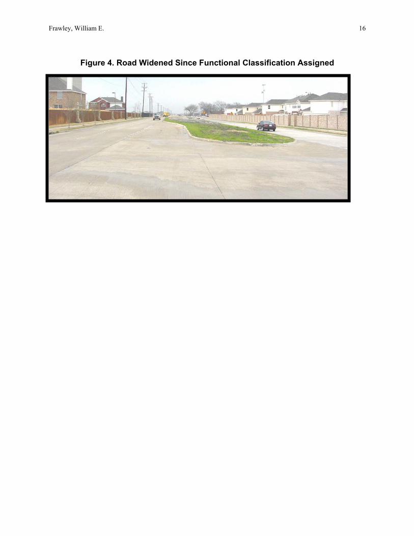
Figure 4 shows an example of a street that has been widened since a functional classification was assigned to it. The volume recorded at this site was 11,072 vehicles.

Another reason that some streets have high volumes is their proximity to specific land uses. Figure 5 depicts a local street that would appear to have low volumes, but does not, due to its proximity to a shopping center shown in Figure 6. The local street in this situation provided a short cut between the shopping center and a principal arterial and had a recorded volume of 12,336 vehicles.

There are numerous land uses that can impact traffic volumes on adjacent streets. Figure 7 shows a local street adjacent to a school, a park with a swimming pool, and an apartment complex. The volume recorded at this street was 11,963.

The vast majority of randomly selected counts had volumes that are more typical of local streets. Figure 8 illustrates an example of residential streets with a volume of 369 vehicles, similar to the median values of the entire area.


QUALITY CONTROL A very important element of this process is quality control. In order to maintain validity, it must be ensured that all counts are actually being performed on streets functionally classified as local. In addition, there must be a sufficient number of usable counts from each area to produce significant results.

Maps – Random Count Selection The process of selecting the count station locations is based on functional classification maps, so the person selecting the count locations immediately knows the functional classification of all roads within a selected grid cell. The count station locations are then transferred to TxDOT’s station location maps so the Tech Services staff can schedule the counts. At least one person not involved in selecting the count sites checks the maps for errors before Tech Services schedules the counts. The person checking the maps verifies that counts were transferred accurately and that all count station locations are actually on streets and not on other facilities, physical features, or boundaries.

Data Collection On occasion, a TTI staff member inspected randomly selected count sites in the field to verify that the counters were set up as close as possible to the exact location chosen. This activity was in response to some data that appeared suspicious (extremely high traffic volumes on streets functionally classified as local). To date all field inspections have shown counts are being collected when and where scheduled.

COUNT RESULTS

Appropriate Sample Sizes Statistical analysis shows different sample sizes are appropriate for various sized urban areas. In every case some count locations selected are not counted due to complications, such as equipment failure, inability to physically set up on a road, or the road may be privately owned. Therefore, more sites than are actually needed should be selected and scheduled to ensure an adequate number of data samples.

The census bureau defines large urban areas as those with populations over 50,000, small urban areas with populations between 5,000 and 50,000, and rural areas as those with populations of less than 5,000. This process separates large urban areas into two groups for considerations of traffic count sample sizes. In large urban areas with populations greater than 200,000, 200 randomly selected sites should yield statistically representative data from at least 150 actual counts. Large urban areas between 50,000 and 200,000 should contain 75 randomly selected sites (yielding at least 50 usable data samples), and small urban areas with populations between 5,000 and 50,000 should have approximately 40 samples selected. The number of samples in small urban areas may vary due to the size of street networks in individual areas. It may be necessary to only schedule 15 or 20 counts in the smallest areas; the person selecting the sites should use discretion in deciding when a system has become saturated with count locations.


In rural areas of counties, including small towns with populations less than 5,000, 33 samples will typically provide statistically valid information; therefore at least 40 sites are should usually be selected. The extra sites selected will allow for bad counts or other problems that prevent data from being collected at specific sites.

Random Count Process Volumes v. Historical Count Location Volumes TTI has compared count volumes from historical TxDOT station locations against count volumes from randomly selected sites within the same areas for several areas around the state. The median values of volumes from randomly selected sites are significantly lower than those of historical counts in the same areas. The volumes at randomly selected sites are consistently lower than volumes at historical station locations primarily because the historical sites are typically located on local streets at or near intersections with collector or arterial streets, where volumes tend to be higher. Historical count sites are not usually found deep in neighborhoods, away from major streets. The randomly selected sites are located on all types of local streets, including cul-de-sacs, and better represent the variety of local streets on the roadway networks.

CONCLUSIONS

Local Street Volume Estimation TxDOT should use a random selection process when performing counts on local streets in order to estimate VMT. This recommendation is supported by the statistical analysis of counts performed in various urban areas that shows the entire local street network is better represented through randomly selected count locations than the historical station locations TxDOT has traditionally used. The historical count locations include bias since they were not originally selected to provide statistically representative traffic volume data. Furthermore, in order to obtain a truly random sample of data each time, new traffic count stations should be randomly selected each time the counts are performed. This element of the process will ensure that any new streets since the last counts have an opportunity to be included in the randomly selected sites.

During the initial years of using this process, TxDOT should consider using a parallel process of counting previous randomly selected sites, new randomly selected sites, and historic sites, to determine if there are any large differences observed in median traffic volumes and growth trends. Inclusion of this element may be determined by budget limitations.

Functional Classification One vital, preliminary observation is that numerous streets exist in some urban areas that have not been classified since construction or reclassified since major improvements have been made. The percentage of misclassified streets varies among urban areas. Some of these streets carry extremely high volumes of traffic, well beyond what would be expected on a local street. This issue must eventually be addressed in some manner, as it relates to local street VMT, to eliminate the unrealistic influence of higher-volume streets. At least two potential responses exist – there may be others:


Response A Reclassify streets that have volumes greater than a certain threshold that all parties can agree upon or determine that the street(s) are actually serving a purpose other than that of a local street. Response B Do not attempt to change functional classification.

Any changes made to functional classification must be done in accordance with all state and federal requirements. Count Reductions By using the random traffic count site selection process, TxDOT has been able to reduce the number of traffic counts it performs across the state by thousands each year. TxDOT eliminates counts on streets functionally classified as local and are not tied to bridges or railroad crossings. These count reductions allow TxDOT to reallocate substantial resources to other count programs.

FUTURE WORK The project team will continue to select and schedule local street count station locations as TxDOT performs future saturation counts. Lessons learned regarding site selection, map work, database construction, field inspection, and data analysis will all be considered as this effort continues.

Future work will also include activities related to quality control, benefiting from lessons learned on being attentive to whether lines on the map are actually roads or other features or boundaries. Project team members will also spot check counter sites in the field as appropriate to ensure that randomness of data is being preserved.

At some point in the future, statewide data will be aggregated in a variety of ways such as by region, population groups, and area types, in order to provide additional useful results.

ACKNOWLEDGEMENTS The author would like to acknowledge the Texas Department of Transportation’s Transportation Planning and Programming Division – Traffic Section, with which the work was conducted through an interagency contract.

REFERENCES 1. Arizona Department of Transportation. Arizona Highway Functional Classification

System: FHWA Guidelines. March, 1989. http://map.azfms.com/advplan/fc_home/guidelines/fc_fhwa_sect_2_1.html. Accessed July 31, 2002.


LIST OF FIGURES

1 Grid Overlay Example

2 TxDOT ACR Station Location Map

3 Houston Area Standard Error vs. Number of Counts

4 Road Widened Since Functional Classification Assigned

5 Road With Land Use Impacts

6 Shopping Center Near High-Volume Location

7 Site With Multiple Adjacent Land Uses

8 Typical (Curvilinear) Residential Local Street


FIGURE 1. MANUAL PROCESS GRID OVERLAY EXAMPLE


Figure 2. TxDOT Station Location Map


Figure 3. Houston Area Standard Error vs. Number of Counts

Houston Non-Attainment Area

(All Area Types)Randomly Selected Counts

0

5

10

15

20

25

30

35

40

45

50

0 50 100 150 200 250 300 350 400 450 500 550 600 650 700 750 800 850 900 950 1,000

Number of Count s


Figure 4. Road Widened Since Functional Classification Assigned


Figure 5. Road With Land Use Impacts


Figure 6. Shopping Center Near High-Volume Local Street Location


Figure 7. Site With Multiple Adjacent Land Uses


Figure 8. Typical (Curvilinear) Residential Local Street

Figure 10. Typical (Grid) Residential Local Street

a methodology for randomly selecting ...frawley, william e. 1 a methodology for randomly selecting...

Documents