A methodology for flexible species distribution modelling within an

Open Source framework

Duncan Golicher∗and Luis Cayuela†

August 29, 2007

Technical report presented to the third International workshop on Species Distri-

bution Modelling financed by the MNP 20-24 August 2007: San Cristobal de Las

Casas, Chiapas, Mexico.

Contents

1 Introduction 3

2 Installing the tools 4

2.1 Installing Linux . . . . . . . . . . . . . . . . . . . . . . . . . . . . . . . . . . . . . . . . . . . . . . . . 42.2 Installing GRASS under Linux . . . . . . . . . . . . . . . . . . . . . . . . . . . . . . . . . . . . . . . 52.3 Installing R . . . . . . . . . . . . . . . . . . . . . . . . . . . . . . . . . . . . . . . . . . . . . . . . . . 62.4 Installing R-packages . . . . . . . . . . . . . . . . . . . . . . . . . . . . . . . . . . . . . . . . . . . . . 72.5 Installing maxent and Google Earth . . . . . . . . . . . . . . . . . . . . . . . . . . . . . . . . . . . . 7

3 Downloading and importing the climate data. 7

3.1 Importing Worldclim data . . . . . . . . . . . . . . . . . . . . . . . . . . . . . . . . . . . . . . . . . . 73.2 Importing VCF data . . . . . . . . . . . . . . . . . . . . . . . . . . . . . . . . . . . . . . . . . . . . . 13

4 Species distribution modelling 14

4.1 Moving climate data from GRASS and visualizing the data . . . . . . . . . . . . . . . . . . . . . . . 144.2 Data reduction using PCA: Producing derived climate layers with R . . . . . . . . . . . . . . . . . . 184.3 Exporting data to ASCII grid and running maxent . . . . . . . . . . . . . . . . . . . . . . . . . . . . 254.4 Comparing maxent results with GAM and CART (rpart) in R . . . . . . . . . . . . . . . . . . . . . 304.5 Investigating the model: Relative importance of the predictor variables . . . . . . . . . . . . . . . . . 324.6 Combining species distribution modelling with multivariate analysis of species association with cli-

mate: The CASP approach . . . . . . . . . . . . . . . . . . . . . . . . . . . . . . . . . . . . . . . . . 37∗El Colegio de La Frontera Sur, San Cristobal de Las Casas, Chiapas Mexico†Universidad de Alcala Henares, Madrid Spain

1

5 Modelling climate change scenarios 45

5.1 Extracting WMO GRIB formatted data . . . . . . . . . . . . . . . . . . . . . . . . . . . . . . . . . . 455.2 Installing CDO . . . . . . . . . . . . . . . . . . . . . . . . . . . . . . . . . . . . . . . . . . . . . . . . 465.3 Obtaining the data . . . . . . . . . . . . . . . . . . . . . . . . . . . . . . . . . . . . . . . . . . . . . . 465.4 Extracting fifty year monthly means . . . . . . . . . . . . . . . . . . . . . . . . . . . . . . . . . . . . 475.5 Exporting to GRASS and visualising the data . . . . . . . . . . . . . . . . . . . . . . . . . . . . . . . 495.6 Downscaling the data . . . . . . . . . . . . . . . . . . . . . . . . . . . . . . . . . . . . . . . . . . . . 525.7 Moving the results to R for modelling . . . . . . . . . . . . . . . . . . . . . . . . . . . . . . . . . . . 54

List of Figures

1 GRASS startup screen . . . . . . . . . . . . . . . . . . . . . . . . . . . . . . . . . . . . . . . . . . . . 102 Setting up a new location . . . . . . . . . . . . . . . . . . . . . . . . . . . . . . . . . . . . . . . . . . 103 Global GRASS region . . . . . . . . . . . . . . . . . . . . . . . . . . . . . . . . . . . . . . . . . . . . 114 Global minimum temperature layer for February at 1km resolution . . . . . . . . . . . . . . . . . . . 135 Mean monthly maximum temperatures across the study region (degrees C) . . . . . . . . . . . . . . 166 Mean monthly minimum temperatures across the study region ( degrees C) . . . . . . . . . . . . . . 177 Mean monthly precipitation across study region (mm) . . . . . . . . . . . . . . . . . . . . . . . . . . 188 Correlations between maximum temperature layers . . . . . . . . . . . . . . . . . . . . . . . . . . . . 209 Correlations between Minimum temperature layers . . . . . . . . . . . . . . . . . . . . . . . . . . . . 2010 Correlations between precipitation layers . . . . . . . . . . . . . . . . . . . . . . . . . . . . . . . . . . 2111 Scree plot of principal components eigenvalues . . . . . . . . . . . . . . . . . . . . . . . . . . . . . . 2212 Visualization of the first four principal components axes mapped onto space . . . . . . . . . . . . . . 2313 Map of the coordinates of 134618 collections of tree species obtained from MOBOT . . . . . . . . . . 2714 Histogram of the log abundances in the collections data . . . . . . . . . . . . . . . . . . . . . . . . . 2815 Maxent GUI . . . . . . . . . . . . . . . . . . . . . . . . . . . . . . . . . . . . . . . . . . . . . . . . . 2916 Example maxent predictive maps for first four species (in alphabetical order) . . . . . . . . . . . . . 3017 Comparisons between GAM, RPart and maxent predictions forAcalypha diversifolia at a regional scale 3318 Maxent response curves for each of the variables used in predicting the distribution of Acalypha

diversifolia . . . . . . . . . . . . . . . . . . . . . . . . . . . . . . . . . . . . . . . . . . . . . . . . . . 3419 GAM response curves for each of the variables used in predicting the distribution of Acalypha diversifolia 3420 Rpart classification tree for Acalypha diversifolia . . . . . . . . . . . . . . . . . . . . . . . . . . . . . 3521 Potential distribution of Acalypha diversifolia as predicted by maxent visualized in Google Earth . . 3722 Overlaying large (10’) quadrats on a the collection data for Nicaragua. . . . . . . . . . . . . . . . . . 3823 Ordination diagram for CCA with climatic contours (tmax6 and prec1) . . . . . . . . . . . . . . . . 4124 Predicted distribution of Climatically Associated Species Pools . . . . . . . . . . . . . . . . . . . . . 4225 Part of the table of abundances of collections of species within the area of each CASP . . . . . . . . 4326 Predicted potential distribution forAcalypha diversifolia based on occurences within CASPS . . . . . 4427 Species richness as suggested by CASP analysis . . . . . . . . . . . . . . . . . . . . . . . . . . . . . . 4528 Startup screen for GRASS showing mapsets for scenario data. . . . . . . . . . . . . . . . . . . . . . . 50

2

29 Predicted change in mean January maximum temperature in the period 2050-2099 compared with1950-1999 (HADCM3 A2) . . . . . . . . . . . . . . . . . . . . . . . . . . . . . . . . . . . . . . . . . . 51

30 Predicted change in mean May maximum temperature in the period 2050-2099 compared with 1950-1999 (HADCM3 A2) . . . . . . . . . . . . . . . . . . . . . . . . . . . . . . . . . . . . . . . . . . . . . 52

31 Artifacts due to large grain of GCM models when simple additive downscaling is used. . . . . . . . . 5332 Additive downscaling preceded by inverse distance weighting interpolation between the centre points

of each GCM cell. . . . . . . . . . . . . . . . . . . . . . . . . . . . . . . . . . . . . . . . . . . . . . . 54

1 Introduction

Using statistical tools to make spatial explicit predictions of distribution is an interesting and informative means offinding relationships between sets of environmental variables and the occurrences of species or sets of species[9]. Themaps that result usually aim to show potential rather than actual distributions[8]. They can be used in the contextof scenario modelling by altering the inputs to the predictive model[13]. The variables used in fitting models areassumed to have spatial distributions that are well enough known to be available in the form of continuous rastercoverages. Efficient algorithms for identifying relationships and mapping the resulting model onto space are widelyavailable and have been implemented within a range of software tools[5]. Once relationships have been identifiedand maps produced the analyst can concentrate on the more complex and interesting task of critically interpretingthe resulting pattern and placing the results in some applied or theoretical context[8].

A common challenge is that preparing all the information and the software tools necessary to reach the stageat which the exercise is productive can be time consuming, especially if a project cannot draw on past experience.Furthermore, while most academic species distribution modelling programs have been made freely available by theauthors, the commercial GIS software used for data preprocessing can be expensive. This cost may represent abarrier for some research groups.

The aim of this document is to provide an easily followed methodology for rapid implementation of speciesdistribution modelling using only open source software. This should allow the reader to reach the stage in whichin depth analysis of the results can begin by drawing our group’s experience. The example is drawn from ourongoing work modelling tree species at a regional (MesoAmerica) scale. Our intention is that the example shouldbe easy to adapt for other projects. Some of the underlying concepts behind species distribution modelling willbe analyzed in the text, but it is not the intention here to provide a detailed technical treatment or analysis ofmodelling algorithms.

The two principal programs that we use are the statistical environment R (http://www.r-project.org)[22], andthe Geographical Information System GRASS (http://grass.itc.it ). These programs both run under MS Win-dows, relying in part on the Unix emulator Cygwin (http://cygwin.com/). In the case of R this dependenceis not visible to most users and R runs well under Windows. However integration between the two programsand the use of system resources are improved greatly when they are run in a Linux environment. Here we firstprovide brief instructions for setting up a complete working system with R and GRASS under Linux. We thendemonstrate how the system can implement several different modelling approaches. The only additional programswe use in the species modelling context are the cross platform java based species modelling program maxent(http://www.cs.princeton.edu/˜schapire/maxent) and the freely available (although not open source) geographicalvisualization program google earth (http://earth.google.com/download-earth.html). Google Earth also runs under

3

Linux.1 The documentation of the project has been prepared using Open Office(http://www.openoffice.org) andtype set using LYX (http://www.lyx.org/)2All programs were run under Ubuntu Feisty 7.04 (http://www.ubuntu.com).The results shown in this document have thus been achieved entirely without the use of software that requires apaid license. A second important element of our approach has been to document all the steps we used in orderto ensure that they can be replicated exactly. This is achieved by the use of scripts rather than run by clickingmenus on a GUI. The software we use is ideal for this. Both R and GRASS are fundamentally command line drivenprograms. This document assumes that the reader is prepared to make full use of all the on line resources availablefor learning Linux, GRASS and R and also read all the appropriate manual pages. It is impossible in the spaceavailable to explain the characteristics of all commands used. The intention is to provide a road map that if followedclosely should lead to repeatable results.

2 Installing the tools

Installing all the software for the project will take around two hours with a good Internet connection. The procedureis not difficult, but may involve some unfamiliar concepts for Windows users.

2.1 Installing Linux

First of all, a brief justification for using Linux is needed. The concept of free software is attractive and the opensource philosophy is compelling. However it may often be worth paying for the features and support provided bycommercial software in the interests of efficient use of time. This is particularly true when it comes to the computeroperating system. This is, after all, no more than a platform to run programs. A perfect operating system wouldcause minimum interruption to the work flow by providing a suitably stable environment with a well integratedset of tools. We have previously carried out a great deal of our modelling work in a more or less satisfactory wayusing GRASS and R in Windows. While R is integral to most of the methods we use, GRASS is not strictlyessential. There are now many good GIS programs available at low cost which are sufficiently powerful for mostspecies distribution modelling. For example the Windows program ILWIS has a great deal of useful functionality.ILWIS is now available free of charge and is also open source under the GPL license (http://52north.org/). HoweverGRASS, arguably, remains the most powerful open source raster based GIS. GRASS is fundamentally a UNIX basedapplication. While GRASS runs adequately in Windows using Cygwin, it is far easier to use and integrate with Rwhen it is run in a Linux environment. We found most contemporary Linux distros to be fast, stable, surprisinglyuser friendly, and above all secure operating systems that are excellent replacements for Windows for every dayuse3.

At the time of writing we consider that the most suitable Linux distro for personal use on a laptop to be UbuntuFeisty 7.04. We reached this conclusion after evaluating SUSE, Slax and a variety of small light weight distros suchas DSL and Puppy. Most can be run through emulation under Windows, but the real advantages are found whenthey are fully installed. The principal virtues of Ubuntu are its simplicity of installation, broad user base, excellent

1We were surprised in fact to find it runs considerably faster.2Using LYX is a simple and effective way to ensure consistent type setting for large documents. It is more stable than using MS Word

or Open Office when documents run to more than 20 pages. A slight drawback is that some characters do not cut and paste correctlyfrom the resulting PDF document to the R console under Windows. Thus we have also provided an unformated text document withall the code and scripts used.

3Both authors of this report have become increasingly frustrated by instability and security issues with Windows operating systems.The first author has switched to Ubuntu for almost all purposes.

4

on line documentation and an attractive user friendly graphical interface which is well designed for use on PCs andlaptops.

In the context of this modelling project an extremely important reason for having Linux, or some other Unixbased operating system, available on at least one computer is that most climate scenario data from Global Circulationmodels is provided in GRIB (machine independent, self descriptive binary format, WMO standard) rather thanASCII grids. This data has to be extracted using specialist software that is compiled and run under Unix. We havesuccessfully installed cdos for this purpose from http://www.mpimet.mpg.de/fileadmin/software/cdo/. We showhow this is used in section 5.

Various flavors of the Ubuntu operating system can be obtained free of charge from http://www.ubuntu.com/and installed from a live CD in around 30 minutes. The minimal requirement is around 6GB of free disk space forthe Linux ext3 partition. Installation is usually a very simple process, and provides comparable functionality toWindows in terms of supported devices (printers, scanners, USB, network etc) “out of the box” although we havehad some problems obtaining optimal screen resolution and sound on some computers. If problems do arise theycan take a while to resolve, but they appear to be rare. However, obviously, repartitioning of a hard disk should notbe contemplated without ensuring full data backup first. We will not repeat the installation instructions providedby Ubuntu here, as they are simple to follow.

Once Ubuntu is up and running and connected to the Internet it is worth taking the time to learn the basics ofthe system from https://help.ubuntu.com/7.04/

2.2 Installing GRASS under Linux

Installing GRASS in Ubuntu is much more straitforward than under Windows. Paste the following lines into theconsole while logged on as root. The simplest way to run as root is to first install the program “Konsole” usingeither

sudo apt-get install konsole

or Add/remove applications .Then begin a session within a new root shell.Be extremely careful when running as root! Usually the prefix “sudo” (super user do) provides root privileges

for a normal user, but parts of the operating system are owned by root and can only be changed when logged on asthe root user. Close the root console as soon as you have finished. Do not type commands that rename or deletefiles from root unless you are quite sure that you know what you are doing.

echo "deb http://les-ejk.cz/ubuntu/ feisty multiverse" > >/etc/apt/sources.list

echo "deb http://us.archive.ubuntu.com/ubuntu/ edgy universe multi-

verse" > >/etc/apt/sources.list

wget -q http://les-ejk.cz/pgp/jachym_cepicky-gpg.pub -O - | sudo apt-key add -

apt-get install grass

We will also need the full gdal package including lbgdal-dev in order to use rgdal to read in and use geographicaldata in R. Gdal is a library with a complete set of functions that other programs can draw on in order to carryout operations such as reprojections and datum shifts. In Windows a compiled version is shipped with rgdal, butgdal must be installed separately in Linux. This can be done most easily using the Synaptic package manager

5

under system administration. Search for and select gdal-bin, libgdal1-dev, libgdal1-grass. Their dependencies areautomatically included.

Alternatively you may paste the following lines into Konsole.

sudo apt-get install gdal-bin

sudo apt-get install libgdal1-dev

sudo apt-get install libgdal1-grass

2.3 Installing R

Installing R follows a similar route. First include a repository in the list of sources for software, confirm that it issafe by adding the key, then update the repositories and install.4

echo "deb http://lib.stat.cmu.edu/R/CRAN/bin/linux/ubuntu/ feisty" > > /etc/apt/sources.list

gpg --keyserver subkeys.pgp.net --recv-key E2A11821

gpg -a --export E2A11821 | sudo apt-key add -

apt-get update

apt-get install r-base

apt-get install r-base-dev

Notice we need two packages, r-base and r-base-dev. The latter package allows us to build additional R packagesfrom source and install them. We have now taken several steps that are not necessary in windows in order toinstall software. By this stage it would be understandable to complain that Linux is unnaturally and unnecessarilycomplicated. The apparent complication comes from the underlying logic of Linux. Windows applications, ingeneral, tend to stand alone in their own folders. There is often a great deal of duplication of functionality betweenthem. This leads to Windows taking up a large amount of disk space. By contrast, Linux is a collection of piecesthat fits together like a jigsaw. Because developers read each others code they make extensive reference to diverselibraries. Compilation of source code prior to installation is also a common practice. This means that operationsthat are complex to achieve in Windows, such as wrapping up some open source C or FORTRAN code within anR package, are comparatively simple. A typical R install in Linux ensures that code libraries are available for use,under the assumption that you might wish to be an R developer as well as a user. Just like a jigsaw, you canbecome extremely frustrated if a piece is missing. That said, all the pieces are available online. Debian distrossuch as Ubuntu are especially good at keeping track of them so you usually can find them all. Once everything isin place it is simply a question of relying on the automated updating process in Ubuntu to keep it all up to date.There is no extra work after the initial set up.

Linux is extremely secure. It is difficult to install anything on line that is not from a trusted source. You musttype in a password to gain administrative privileges before you can make any changes. This makes Linux a naturallyvirus free operating system. Also, if you were new to Ubuntu, you should have noticed by now that for routine usethe GUI is at least as intuitive and simple to use as Windows. The use of scripts is simply a convenient way ofproviding information. It is possible to use the GUI for almost every common task.

4Both R and GRASS can be installed quickly and painlessly with all their dependencies using the synaptic GUI. However the defaultbehavior of Synaptic is to install old versions, under the assumption that newer versions are unstable. In the case of R this means thatnew loaded packages won’t work.

6

2.4 Installing R-packages

The R language is extended by the use of installed packages. All installs in Linux require the appropriate privilegesthe process of installation is slightly more complex than under Windows. It is important to ensure that all packagedependencies are installed and compilable. There are occasional frustrations with missing libraries or compilersthat require tracking down5. This can be a particular problem with spatial packages. To install the R packages wewill use we again use the root shell in Konsole. On opening the root shell type “R” to run R and then from withinR type:

install.packages(c("spgrass","vegan","mgcv","mda","gam","rpart,"RColorBrewer"),dep=T)

2.5 Installing maxent and Google Earth

Finally download maxent.jar from http://www.cs.princeton.edu/˜schapire/maxent/ and save the file in a directorycalled “maxent” within your home directory. There is no need to install the program, it should run using thepreinstalled version of Java in Ubuntu. If not, install Sun-java version 6 using Synaptics. If your computer has asuitable graphics card installed it can run Google Earth. Download the binary and cd to the directory in which itwas saved. It can then be installed with:

sudo sh ./GoogleEarthLinux.bin

This should complete the installation of all the basic tools. Before starting modelling we need data.

3 Downloading and importing the climate data.

The quality and accuracy of the climatic coverage will have an important effect on modelled results. It is thusimportant to use a high quality and consistent data source across projects.

3.1 Importing Worldclim data

We have found that for relatively high resolution modeling (the highlands of Chiapas) direct interpolation fromlocally available climate data is probably the best way of obtaining continuous climate coverages. This has theadvantage of allowing direct control over the interpolation process in order to ensure that the effects of elevationcan be treated in a way that is consistent with the locally acting processes such as temperature lapse rate and rainshadow effects. However modeling at the larger regional scale requires the use of a global data set. A widely usedhigh quality data set is available from the worldclim site.

http://www.worldclim.org/current.htmThis data has been checked for quality and represents a very valuable resource. We include a brief description

of this data set by the authors[14].

The data layers were generated through interpolation of average monthly climate data from weatherstations on a 30 arc-second resolution grid (often referred to as ”1 km” resolution). Variables included

5We have found that missing dependency problems in general are very rare when using Ubuntu, but care does have to be taken wheninstalling R packages.

7

are monthly total precipitation, and monthly mean, minimum and maximum temperature, and 19derived bio-climatic variables.

The WorldClim interpolated climate layers were made using: Major climate databases compiled bythe Global Historical Climatology Network (GHCN), the FAO, the WMO, the International Center forTropical Agriculture (CIAT), R-HYdronet, and a number of additional minor databases for Australia,New Zealand, the Nordic European Countries, Ecuador, Peru, Bolivia, among others. The SRTMelevation database (aggregated to 30 arc-seconds, ”1 km”) The ANUSPLIN software.

ANUSPLIN is a program for interpolating noisy multi-variate data using thin plate smoothing splines.We used latitude, longitude, and elevation as independent variables. For stations for which we hadrecords for multiple years, we calculated averages for the 1960-90 period. We only used records forwhich there were at least 10 years of data. In some cases we extended the time period to the 1950-2000period to include records from areas for which we had few recent records available (e.g., DR Congo) orpredominantly recent records (e.g., Amazonia). We started with the data provided by GHCN, becauseof the high quality of that database. We then added additional stations from other database. Manyof these additional databases had mean monthly values, without a specification of the time period.We added these records anyway, to obtain the best possible spatial representation, reasoning that inmost cases these records will represent the 1950-2000 time period, and that insufficient capture ofspatial variation is likely to be a larger source of error than in high resolution surfaces than than effectsclimatic change during the past 50 years. After removing stations with errors, our database consistedof precipitation records from 47,554 locations, mean temperature from 24,542 locations, and minimumand maximum temperature for 14,835 locations (see maps below). A set of ’Bioclimatic variables’ werederived from the monthly data. Bioclimatic variables are derived from the monthly temperature andrainfall values in order to generate more biologically meaningful variables. These are often used inecological niche modeling (e.g., BIOCLIM, GARP). The bioclimatic variables represent annual trends(e.g., mean annual temperature, annual precipitation) seasonality (e.g., annual range in temperatureand precipitation) and extreme or limiting environmental factors (e.g., temperature of the coldest andwarmest month, and precipitation of the wet and dry quarters). A quarter is a period of three months(1/4 of the year). They are coded as follows:

� BIO1 = Annual Mean Temperature

� BIO2 = Mean Diurnal Range (Mean of monthly (max temp - min temp))

� BIO3 = Isothermality (P2/P7) (* 100)

� BIO4 = Temperature Seasonality (standard deviation *100)

� BIO5 = Max Temperature of Warmest Month

� BIO6 = Min Temperature of Coldest Month

� BIO7 = Temperature Annual Range (P5-P6)

� BIO8 = Mean Temperature of Wettest Quarter

� BIO9 = Mean Temperature of Driest Quarter

8

� BIO10 = Mean Temperature of Warmest Quarter

� BIO11 = Mean Temperature of Coldest Quarter

� BIO12 = Annual Precipitation

� BIO13 = Precipitation of Wettest Month

� BIO14 = Precipitation of Driest Month

� BIO15 = Precipitation Seasonality (Coefficient of Variation)

� BIO16 = Precipitation of Wettest Quarter

� BIO17 = Precipitation of Driest Quarter

� BIO18 = Precipitation of Warmest Quarter

� BIO19 = Precipitation of Coldest Quarter

In order to use this data we will take advantage of the power of GRASS to handle extremely large raster coveragesthrough its use of regions. We can import the whole global “1 km2”data set at once and then easily work on subsetsfor different regions with different resolutions. This is simpler in GRASS than any other GIS that we know of. It isthe feature that makes GRASS particularly well suited for large projects using extensive data sets. GRASS is alsoextremely rigorous in its use of datum and projection because of the location concept. A location contains a set ofcoverages that must be in the same projection.

Before starting GRASS you need a suitably large disk space to store the data. We use external removal USBdrives for geographical data to avoid filling up the fixed hard drive. Linux does not use drive letters. Instead drivesare treated as directories by being mounted at any point in the directory structure. If the drive is not mountedautomatically, right clicking the drive shown in ”computer” allows you to mount the drive in the default positionand it appears on the desktop. This is convenient for unmounting before removal.The first disk receives the namedisk, then disk-1, disk-2 etc. In the example here a partition receives the name ”disk”, so a mounted usb drive isgiven media/disk-1. Make a directory on the mounted disk either using Nautilus in a similar manner as you wouldusing Explorer in Windows. Alternatively type in the Konsole:

mkdir /media/disk-1/GRASSDATA

Throughout the document lines marked in red may be changed to reflect differences in the directory structure ormount points between machines. Now start GRASS by typing grass62. Browse to the directory where you will keepall the data. You cannot enter GRASS until you have added the first location. A GRASS location contains a set ofdata with identical projection parameters. Thus the term ”location” might be slightly misleading. In this case ourlocation will be global. Select ”Projection values” from the startup screen (Figure 1)

9

Figure 1: GRASS startup screen

After the startup screen you need to name the Location and Mapset. Each location has a PERMANENT mapsetthat contains shared data. As the climatic layers are fundamental ingredient for species distribution modelling theyshould be in the PERMANENT mapset (Figure 2).

Figure 2: Setting up a new location

Once you have entered the location answer the questions forming a location with coordinate system Latitudeand Longitude (B), geodetic datum wgs84 and ellipsoid wgs84. Then fill in the global boundaries of the location asin figure 3.

10

Figure 3: Global GRASS region

Once you are in GRASS all the data that is already imported into the system will come from within the locationyou used when entering. Moving between locations involves exiting from GRASS and re-entering. This is a verygood feature that automatically prevents you attempting to combine data that is incompatible if other locationsuse different projections and datums. Reprojection involves moving data between locations and reprojecting them.

One concept that might seem strange is that while you are “in” GRASS you are also running a bash shell. Thismakes all the usual system commands available including running other programs from within GRASS. We use thisto mix GRASS and R code later. When importing data into GRASS you can move to the directory where datawas stored using the usual cd command. This does not change the fact that you are still working within the samelocation and database. So importing data usually involves moving to the directory where it was stored then issuingthe appropriate commands to bring it into GRASS and reproject if necessary. Gdal is vital to this process.

We assume that the data has been downloaded from http://www.worldclim.org/current.htm in its original formatand unzipped to a directory called worldclim. Each of these very large files can then be unzipped to a separatedirectory and named accordingly. Because of the size of the files this takes some time and requires around 1GB offree space for each unzipped layer. Unless you have a very large hard disk it will be necessary to unzip a set at atime and then delete the unzipped files after importing the data to GRASS. Fortunately the files are recompactedupon importation into GRASS so the final assembled data base on completion is not so large. The following linesimport twelve data layers into GRASS that have been extracted into a directory named tmax. This can be done“by hand” using the GRASS GUI, but it is much more convenient to take advantage of the consistent naming of thefiles and build a very simple shell script as importation can take some time due to the size of the files. Note againthat you may need to change the line marked in red to reflect your own choice of mount point and directory.

cd /media/disk-1/worldclim/tmax

for i in $(seq 1 12)

do

r.in.bin -s input=tmax_$i.bil output=tmax$i bytes=2 north=90 south=-

60 east=180 west=-180 rows=18000 cols=43200 anull=-9999

done

This ability to mix shell commands with GRASS commands is extremely powerful and makes GRASS easier toscript than most other GISs. A bonus is that by doing so you learn a syntax which is very useful for automatingother tasks in Linux.

The process can be repeated for all the other climate layers.

11

cd /media/disk-1/worldclim/tmin

for i in $(seq 1 12)

do

r.in.bin -s input=tmin_$i.bil output=tmin$i bytes=2 north=90 south=-

60 east=180 west=-180 rows=18000 cols=43200 anull=-9999

done

cd /media/disk-1/worldclim/prec

for i in $(seq 1 12)

do

r.in.bin -s input=prec_$i.bil output=prec$i bytes=2 north=90 south=-

60 east=180 west=-180 rows=18000 cols=43200 anull=-9999

done

cd /media/disk-1/worldclim/bio

for i in $(seq 1 19)

do

r.in.bin -s input=bio_$i.bil output=bio$i bytes=2 north=90 south=-60 east=180 west=-

180 rows=18000 cols=43200 anull=-9999

done

Finally import the elevation data from the same source

r.in.bin -s input=alt.bil output=alt bytes=2 north=90 south=-60 east=180 west=-

180 rows=18000 cols=43200 anull=-9999

This process will have taken several hours, but you will now have a major resource ready for species distributionmodelling anywhere in the world in a convenient format. To visualize a layer either use the GRASS GUI, or opena monitor to obtain the results shown in figure 4.

d.mon start=x0

d.mon select=x0

d.rast tmin2

12

Figure 4: Global minimum temperature layer for February at 1km resolution

To select any subset of this data simply use the interactive zoom to set the new region limits.

d.zoom

To lower the resolution through nearest neighbor (taking the value closest to the centre of the new cell) resamplinguse

g.region res=00:03

All the data layers will now be clipped to the new region and use cells of approximately 5km x 5km. This newregion will be respected next time you enter GRASS. Be careful when importing data as the default is to onlyimport data that falls within this current region. To reset to the region used for the worldclim coverages use (forexample); g.region rast=tmin2. The region concept is one of the great strengths of GRASS as it allows fast andclean subsetting of a very large global data set such as this, but it does require a little experience to get used to theway it works. Notice that you can increase the resolution to greater than the original, but this will obviously notresult in any increase in the level of detail. Notice also that GRASS can run complex calculations on these verylarge raster coverages extremely quickly.

3.2 Importing VCF data

A second useful type of data is derived from satellite imagery. At the large regional scale Modis data is mostappropriate. The Vegetation Continuous Fields collection [11, 13] contains proportional estimates for vegetativecover types: woody vegetation, herbaceous vegetation, and bare ground. The product is derived from all sevenbands of the MODerate-resolution Imaging Spectroradiometer (MODIS) sensor onboard NASA’s Terra satellite.

According to the authors the continuous classification scheme of the VCF product may depict areas of hetero-geneous land cover better than traditional discrete classification schemes. While traditional classification schemesindicate where land cover types are concentrated, this VCF product is good for showing how much of a land coversuch as ”forest” or ”grassland” exists anywhere on a land surface.

The version four coverage can be downloaded from

13

http://glcfapp.umiacs.umd.edu:8080/esdi/index.jspThe three data files included are percent trees, bare, and herbaceous. This product contains three available

layers which add up to represent 100% ground cover. The first layer represents percent tree cover, the secondrepresents percent herbaceous ground cover. and the third layer represents percent bare ground cover. The threelayers can be properly displayed in a Red, Green, Blue band combination.

Although it is in Lat Long format the datum and projection (according to the header the datum is not specifiedbut based on an authalic sphere. If imported directly the coordinates do not match those of the WorldClim dataso a new location needs to be produced.

r.in.gdal input=LatLon.NA.2001.bare.tif output=VCFBare title=bare location=VCF

Now exit GRASS and re-enter in the new location called VCF.

r.in.gdal input=LatLon.NA.2001.herbaceous.tif output=VCFHerb

r.in.gdal input=LatLon.NA.2001.tree.tif output=VCFTree

Now the data can be reprojected within the same location as the WorldClima data.

g.region res=00:00:30

r.proj input=VCFHerb location=VCF output=VCFHerb method=nearest

r.proj input=VCFTree location=VCF output=VCFTree method=nearest

r.proj input=VCFBare location=VCF output=VCFBare method=nearest

Once these data have been imported into the PERMANENT mapset a new mapset can be produced that is focusedon the region for modelling.

Within the mapset the cell resolution can be set to 3 arc minutes to use cell sizes of approximately 5km x 5km.

g.region res=00:03

4 Species distribution modelling

4.1 Moving climate data from GRASS and visualizing the data

R can be started within GRASS and data moved easily between the two programs using spgrass6. Because R holdsall data in memory there are limits to the size of the data that can be be handled at once. This is potentially adrawback of R for handling very large raster layers. However at this resolution there are no problems running Runder Ubuntu (or Windows) on a laptop with 1GB of RAM.6

1. First enter GRASS and set the region and resolution. Then type R in order to start R. Load the packagespgrass6. The complete set of climate coverages with the exception of the derived bioclim layers can be readinto memory using:

6Some species modelling algorithms could be run in GRASS directly, and GRASS can work with extremely large raster layers heldon disk. However R has statistical abilities that are not included in a GIS. The long term solution for working with very large data setswill be to run R in a 64 bit environment with extra memory.

14

library(spgrass6)

a<-paste("tmax",1:12,sep="")

a<-c(a,paste("tmin",1:12,sep=""))

a<-c(a,paste("prec",1:12,sep=""))

clima<-readRAST6(a)

We save this data as an R binary object for future use in the working directory.

save (clima, file="climaSGDF.rob")

The default spatial object is a fully gridded SpatialGridDataFrame, in other words it is in the form of a rectangularmatrix with NAs filling the blank regions. For many analysis a better form is a SpatialPixelsDataFrame which onlyholds cells with values and has a separate component for the cell coordinates. This is more efficient in the case ofthe long thin shape of the study area. The conversion takes some time so we will run it once and save the resultsas a separate object. It will then be quicker to move between the two forms by reloading the objects.

fullgrid(clima)<-F

save(climaSPDF,rob)

The binary objects formed by the save command can be reloaded by R running under either Linux or Windows. Soat this stage it is possible to run the rest of the analysis using R under Windows if this is preferred.

We have 36 layers in the object climaSPDF However we will not use all these as they share too much infor-mation. This is also the case for the derived bioclim layers which we could have also imported at this stage. Wehave investigated the properties of bioclim and decided that on balance it is preferable to begin with the easilyinterpretable rainfall and temperature layers and selectively derive layers from them using R. There are severalreasons for this decision.

1. Direct downscaling of climate change scenarios is a much more transparent process if the original monthlymeans are used as input.

2. Some of the original bioclim layers have rather poor statistical properties due to disjunctions. This is aparticular problem with layers such as the precipitation of the warmest month or the temperature of thewettest month. These layers tend to have linear breakpoints, especially in northern Mexico where there isa shift between a Mediterranean type climate with most precipitation falling in the winter months, to asubtropical climate with summer rainfall. While the interpretation of the bioclim layers in terms of factorsdetermining plant growth captures this well, the layers that are produced tend to lead to predictive modelswith overly sharp boundaries.

3. With the possible exception of the layers mentioned above, bioclim layers are highly correlated and share agreat deal of information.

We will now show how to use the power of R to quickly build customized bioclimatic coverages using the data andlook at the data as maps in R. One of the nice features is that all the maps can be plotted at once using the samecolour scale, something that is not easily achieved using a GIS. We can also carry out extremely fast flexible datamanipulation. In this case the temperature data were originally multiplied by ten in order to be stored as integersin the WorldClim database. They can all be changed back with a single line.

15

clima@data[,1:24]<-lapply(clima@data[,1:24],function(x)x/10)

Now we can visualize the data.

png(file="tmax.png")

trellis.par.set(sp.theme())

print(spplot(clima,c(1:12)))

dev.off()

Figure 5: Mean monthly maximum temperatures across the study region (degrees C)

png(file="tmin.png")

trellis.par.set(sp.theme())

print(spplot(clima,c(13:24)))

dev.off()

16

Figure 6: Mean monthly minimum temperatures across the study region ( degrees C)

png(file="prec.png")

trellis.par.set(regions=list(col=terrain.colors(100)[100:1]))

print(spplot(clima,c(25:36)))

dev.off()

17

Figure 7: Mean monthly precipitation across study region (mm)

From figures 5, 6 and 7 we can see that there are fundamentally four elements to the climatic variability over theregion. There is a strong latitudinal seasonal effect that is particularly marked in Mexico. Northern Mexico fallsabove the tropic of cancer and has marked annual temperature fluctuations. This seasonality extends into thesub-tropical zones due to the influence of air movements associated with cold fronts in the winter months. Coldfronts affect the Gulf coast much more strongly than the Pacific Coast.

4.2 Data reduction using PCA: Producing derived climate layers with R

In order to look for ways to reduce the dimensionality of the data it can useful to plot the correlations betweenlayers. We use a customized pairs plot that can be run after the following code has been pasted or sourced into R.

panel.line<- function (x, y, col = par("col"), bg = NA, pch = par("pch"),

cex = 1, ...)

{

points(x, y, pch = pch, col = col, bg = bg, cex = cex)

18

ok <- is.finite(x) & is.finite(y)

if (any(ok))

md<-step(lm(y~poly(x,2)))

xx<- seq(min(x),max(x),length=100)

yy<-predict(md,data.frame(x=xx),se=T,type="response")

lines(xx,yy$fit,col=1)

lines(xx,yy$fit+2*yy$se.fit,col=3,lty=2)

lines(xx,yy$fit-2*yy$se.fit,col=2,lty=2)

}

panel.hist <- function(x, ...)

{

usr <- par("usr"); on.exit(par(usr))

par(usr = c(usr[1:2], 0, 1.5) )

h <- hist(x, plot = FALSE)

breaks <- h$breaks; nB <- length(breaks)

y <- h$counts; y <- y/max(y)

rect(breaks[-nB], 0, breaks[-1], y, col="cyan", ...)

}

panel.cor <- function(x, y, digits=2, prefix="", cex.cor)

{

usr <- par("usr"); on.exit(par(usr))

par(usr = c(0, 1, 0, 1))

r <- abs(cor(x, y))

txt <- format(c(r, 0.123456789), digits=digits)[1]

txt <- paste(prefix, txt, sep="")

if(missing(cex.cor)) cex <- 0.8/strwidth(txt)

text(0.5, 0.5, txt, cex = cex * r*2)

}

Xpairs<-function(...)pairs(...,lower.panel=panel.line, up-

per.panel=panel.cor,diag.panel=panel.hist)

Now we can look at the correlations between data layers.

Xpairs(clima@data[,1:12])

19

Figure 8: Correlations between maximum temperature layers

Xpairs(clima@data[,13:24])

Figure 9: Correlations between Minimum temperature layers

Xpairs(clima@data[,25:36])

20

Figure 10: Correlations between precipitation layers

Figures 8,9 and 10 show correlation coefficients between layers in a font size which is proportional to the size of thecorrelation, allowing a quick impression of the patterns. If the layers are ”information rich” correlations betweenthem are small. The greater the correlation the less independent information. Over a small region such as thehighlands of Chiapas or even Nicaragua temperatures will tend to be simple linear functions of altitude so alltemperature layers will be very highly correlated. In fact part of this correlation can be explained by the use of alapse rate model or linear regression against elevation in order to derive the layers using either Kriging or Anusplin.At the scale of this data set the layers are more information rich. The highest correlations are between months closetogether and there seems little to be gained by using more than two to four months.

There is always a certain tension in predictive modeling between the use of predictors with good statisticalproperties and those that are easily interpretable in terms of processes known to be predictive in an ecologicalsense. Niche models typically aim to be interpretable in ecological terms. However it can happen that the desireto produce models that use factors that a priori influence a species distribution leads to an analyst overlookingthe limitations to orthogonality in the data. For example if, over a comparatively small area, warmer temperaturesare always associated with moister conditions it will be impossible to separate which factor determines a speciesdistribution from data alone. It is worth analyzing the statistical property of co-linearity using principal componentsanalysis before deciding on the data layers to use.

Principal component analysis (PCA) is primarily a dimension-reduction technique, which takes observationson p correlated variables and replaces them by uncorrelated variables. These uncorrelated variables, the principalcomponents (PCs), are linear combinations of the original variables, which successively account for as much aspossible of the variation in the original variables. Typically a number m is chosen (m << p) such that using onlythe first m PCs instead of the p variables will involve only a small loss of variation. The vectors of loadings whichdefine the PCs are known as empirical orthogonal functions (EOFs). One problem with using PCA to replace pvariables by m PCs, rather than the alternative strategy of replacing the p variables by a subset of m of the originalvariables, is interpretation. Each PC is a linear combination of all p variables, and to interpret a PC it is necessary

21

to decide which variables are important, and which are unimportant, in defining that PC. It is common practiceto rotate the EOFs. This idea comes from factor analysis, and proceeds by post-multiplying the (p Ö m) matrixof PC loadings by a (usually orthogonal) matrix to make the loadings ‘simple’. Simplicity is defined by severalcriteria (e.g. varimax, quartimax) which quantify the idea that loadings should be near zero or near ±1, with asfew as possible intermediate values. Rotation takes place within the subspace defined by the first m PCs. Hence allthe variation in this subspace is preserved by the rotation, but it is redistributed amongst the rotated components,which no longer have the successive maximization property of the unrotated PCs. What this means in effect is ifrotation can produce a pattern of loadings approaching ±1 on each of the variables then the original variables canbe used instead of PCs, thus retaining interpretability.

The following R code produces a pca object in R and maps the results onto space as shown in figure 12.

pca<-princomp(clima@data,cor=T)

plot(pca)

Figure 11: Scree plot of principal components eigenvalues

pca.sp<-clima

pca.sp@data<-as.data.frame(pca$scores[,1:4])

trellis.par.set(sp.theme())

spplot(pca.sp)

22

Figure 12: Visualization of the first four principal components axes mapped onto space

Figure 12 suggests that PCA 1 is perhaps interpretable as an overall index of ”tropicality” in a broad sense withorange and red colours suggesting greater seasonality and perhaps cooler winter temperatures. Component 2 seemsto be interpretable as capturing mainly variability in precipitation with orange and red marking areas with higherrainfall. The other layers do not seem to have a particularly obvious interpretation. Looking at the loadings aftervarimax transform helps to clarify what the PCA is capturing.

> varimax(pca$loadings[,1:4])

$loadings

Loadings:

Comp.1 Comp.2 Comp.3 Comp.4

tmax1 -0.289

tmax2 -0.301

tmax3 -0.308

tmax4 -0.111 -0.307

tmax5 -0.246 -0.271

tmax6 0.122 -0.360 -0.102

tmax7 -0.352

tmax8 -0.337

tmax9 -0.327

tmax10 -0.259 -0.158

tmax11 -0.290

tmax12 -0.284

tmin1 -0.248

tmin2 -0.258

tmin3 -0.267

23

tmin4 -0.268

tmin5 -0.251

tmin6 -0.194 -0.175

tmin7 -0.174 -0.246

tmin8 -0.193 -0.236

tmin9 -0.213 -0.182

tmin10 -0.245

tmin11 -0.258

tmin12 -0.250

prec1 0.363

prec2 0.383

prec3 0.367

prec4 0.286

prec5 -0.142 0.103 0.171

prec6 0.140 0.164 -0.162

prec7 0.144 0.252 -0.258

prec8 0.122 0.234 -0.266

prec9 0.123 0.138 -0.189

prec10 0.203

prec11 0.294

prec12 0.364

SeasonalMaxTDif 0.138 -0.267 0.182

DailyTDif 0.417 -0.269

GrowingMonths 0.116 0.183 -0.111

Now the interpretation of the third component becomes slightly clearer. While Tabasco and Baja California haveradically different climates, they share the fact that some rain falls during the winter. This shows a potential dangerof using simple linear combinations of variables for modelling.

We can use the power of R to quickly process data held as spatial objects to hopefully find some more informativeclimatic layers similar to the bioclim layers. The advantage of writing our own code to do this is that bioclimaticlayers can be easily re-derived from downscaled climate change scenarios. It is also worth basing the derived layersat least loosely on the results of the PCA analysis in order to aim for orthogonality. This seems to suggest thatmaximum orthogonality can be produced by looking at seasonal differences and daily temperature differences. Thenumber of months with more than 100mm of rain might be a very simple way of estimating the length of the growingseason. 7

f<-function(x)max(x[1:12])-min(x[1:12])

clima[["AnnualMaxTDif"]]<-apply(clima@data,1,f)

f<-function(x)max(x[1:12]-x[13:24])

clima[["DailyTDif"]]<-apply(clima@data,1,f)

7More complex methods involve calculating evapotranspiration.

24

f<-function(x)sum(x[25:36]>100)

clima[["GrowingMonths"]]<-apply(clima@data,1,f)

We can select some of the key variables identified in the PCA along with the derived variables and form a new climaobject.

clima2<-clima

clima2@data<-clima2@data[,c(6,13,25,30,37,38,39)]

Now we can look at a PCA of the derived variables.

pca2<-(princomp(clima2@data,cor=T))

loadings(pca2)

Loadings:

Comp.1 Comp.2 Comp.3 Comp.4 Comp.5 Comp.6 Comp.7

tmax6 -0.178 0.838 -0.198 -0.284 0.381

tmin1 0.404 0.326 -0.421 -0.266 -0.128 -0.679

prec1 0.326 0.238 0.799 -0.104 -0.372 -0.224

prec6 0.430 -0.352 0.685 -0.468

AnnualMaxTDif -0.401 0.302 0.373 0.210 0.511 0.146 -0.531

DailyTDif -0.392 -0.199 -0.810 -0.198 -0.332

GrowingMonths 0.447 -0.283 0.146 0.832

The loadings look a lot better. In fact upon rotation we can identify a unique interpretation for each axis, so theoriginal variables do indeed possess enough orthogonality to be useful for modelling without being substituted forPCA axes. This allows much clearer interpretation.

varimax(loadings(pca2))

Loadings:

Comp.1 Comp.2 Comp.3 Comp.4 Comp.5 Comp.6 Comp.7

tmax6 1

tmin1 -1

prec1 1

prec6 1

AnnualMaxTDif -1

DailyTDif -1

GrowingMonths 1

We seem to have found an almost perfect combination of variables that can be used instead of PCs.

4.3 Exporting data to ASCII grid and running maxent

The software for maximum entropy modelling forms a useful tool for species distribution modelling which has agood user interface and seems to outperform the previously most popular software for modelling occurrence onlydata, GARP, certainly in speed and arguably in predictive ability[16]. Once a subset of climatic layers has been

25

decided on for modelling exporting the layers to a format that maxent can use is extremely straitforward. Changethe first line of the following code to the directory in which maxent.jar was saved.

maxentpath<-"/home/duncan/SpeciesModels/maxent"

dir.create(paste(maxentpath,"clima",sep="/"))

for (i in 1:7){

fname<-paste(names(clima2@data)[i],"asc",sep=".")

fname<-paste(maxentpath,"clima",fname,sep="/")

writeAsciiGrid(clima2, fname, attr = i)

}

Now we need to load some species occurrence data and overlay it on the climate data. The data is a subset ofthe total data we are using and has been derived from querying the Missouri Botanical Garden’s VAST data basehttp://mobot.mobot.org/W3T/Search/vast.html using a list of tree species found from southern Mexico to Panama.It can be loaded using

d<-read.table("SMesoTrees.txt",header=T)

Now we can quickly look at the characteristics of the data with str

str(d)

’data.frame’: 134618 obs. of 8 variables:

$ Name : Factor w/ 3140 lev-

els "Abarema_barbouriana",..: 24 24 24 24 24 24 35 35 35 35 ...

$ Place : Factor w/ 159 levels "Belize ","Be-

lize : 0",..: 140 140 140 140 156 156 10 10 10 12 ...

$ x : num -79.9 -79.8 -79.8 -79.9 -79.4 ...

$ y : num 9.16 9.15 9.16 9.17 9.40 ...

$ Year : Factor w/ 154 lev-

els "1094","1825",..: 115 154 79 81 133 132 120 121 120 102 ...

$ Political: logi FALSE FALSE FALSE FALSE FALSE FALSE ...

$ Genus : Factor w/ 803 levels "Abarema","Abies",..: 4 4 4 4 4 4 5 5 5 5 ...

$ Species : Factor w/ 1961 levels "acapul-

cense",..: 1103 1103 1103 1103 1103 1103 542 542 542 542 ...

From this we can see that we have 134618 observations on the locations from which 3140 species have been collected.Data with only ”Political” locations, i.e. municipalities or states have already been removed from this data so the”Political” column is a legacy. Although there seems to be a lot of information there are serious issues for successfulspecies distribution modelling. One problem is that some of the coordinates are dubious. This can be seen mosteasily by plotting the points.

library(mapdata)

map("worldHires",c("Mexi","Costa Ri","Panama","El Sal-

vad","Hondur","Nicara","guate","Beliz"))

26

points(d$x,d$y,pch=21,bg=2,cex=0.4)

box()

axis(1)

axis(2)

grid()

Although there are some islands with trees of the coast, a few points are quite obviously errors in figure 13.

Figure 13: Map of the coordinates of 134618 collections of tree species obtained from MOBOT

We can also look at the distribution in the number of collections per species quickly using the histogram of atable. Table in R produces a table of abundances. If we use the log to the base ten the results are easily interpretable.The distribution is shown in figure 14. Note that the median number of collections per species is 18 and 25% havefive or less. Although species distribution maps can be built from a very small number of collections, their validityis very doubtful. Furthermore the fewer the number of data points the higher the possibility of the results beingseriously biased by errors in geopositioning of the points.

hist(log10(table(d$Name)))

summary(as.vector(table(d$Name)))

Min. 1st Qu. Median Mean 3rd Qu. Max.

1.00 5.00 18.00 42.87 48.25 1027.00

27

Figure 14: Histogram of the log abundances in the collections data

We will now sort the data by abundance and overlay the points on the climate layers.

d$Name<-factor(d$Name,names(sort(table(d$Name),d=T)))

d<-d[order(d$Name),]

coordinates(d)<-~x+y

d<-data.frame(d,clima2@data[overlay(clima2,d),])

d<-na.omit(d)

This code is concise and there are some rather subtle R tricks that are used here that may not be obvious evenfor more experienced R users8. The first line takes the factor ”Name” and places the levels in order with the mostfrequent species first, the default being for factor levels to be in alphabetical order. The second line then ordersthe whole data frame according to the factor levels. The third line changes (temporarily) the data frame into aSpatialPointsDataFrame which allows the overlay to work in the fourth line. Then the final line does quite a lot ofwork all at once. Overlay of clima2 on d produces a numerical array of indices of clima2 on locations of d. This isthen used to select rows of the data frame clima2@data9 which are annexed to the original data frame. The finalline removes any data points which fall outside the overlay.

Now we can export some of the species for maxent modelling. First we check the path to the directory containingmaxent.jar. There should already be a subdirectory with the climate data. We then select the hundred mostabundant species from the list for modelling and form a file called ”mostabun.csv” from them. Then we can startup maxent directly from R (under windows use the command ”shell” instead of system.)

maxentpath<-"/home/duncan/SpeciesModels/maxent"

dir.create(paste(maxentpath,"results1",sep="/"))

8One of the features of the R language is that work that would take a large number of lines of code in other languages can becondensed into a single line. This is particularly true when the ”apply” family is used, but can also arise from multiple subsetting of asin this example.

9Formally the preferred way to access information held in the slots of S4 classes is through methods rather than extracting ”manually”in this way. However we have found that the data method for spatial classes is not always available. For scripting purposes this formof extraction appears to be preferable.

28

nsp<-100

subsetd<-subset(d,d$Name%in%names(sort(table(d$Name),decreasing=T))[1:nsp])

subsetd<-data.frame(name=subsetd$Name,long=subsetd$x,lat=subsetd$y)

write.table(subsetd,sep=",",file=paste(maxentpath,"mostabun.csv",sep="/"),row.names=F)

setwd(maxentpath)

cmd<-"java -jar maxent.jar -K -

P environmentallayers=clima samplesfile=’mostabun.csv’ outputdirectory=results1"

system(cmd)

This should start up maxent as shown in figure 15. Selecting the jacknife measure of variable importance can beuseful, but slows the modelling quite considerably so we will first get some output without.

Figure 15: Maxent GUI

The results can now be looked at and analyzed in the directory setup for them. We can also read the ASCIIgrids back into R and visualize them there. Make sure the ”d” object that was set up previously is available asthe points from this are overplotted. Figure 16shows some example results for the first four species in alphabeticalorder.

setwd(paste(maxentpath,"results1",sep="/"))

a<-dir()

a<-a[grep("\\.asc",a)]

library(mapdata)

for (i in 1:10){

aa<-readAsciiGrid(a[i])

map("worldHires",c("Costa Ri","Panama","El Sal-

vad","Hondur","Nicara","Guate","Beliz"))

aa[[1]][aa[[1]]<30]<-NA

image(aa,col=brewer.pal(7,"Greens"),add=T)

s<-subset(d,d$Name==gsub(".asc","",a[i]))

29

points(s$x,s$y,pch=21,bg=2,cex=0.5)

title(main=gsub(".asc","",a[i]))

}

Figure 16: Example maxent predictive maps for first four species (in alphabetical order)

4.4 Comparing maxent results with GAM and CART (rpart) in R

It is interesting to compare the results from maxent with some of the various other methods that can be implementedin R. R has a very large range of predictive modelling techniques available but we will concentrate here on just twopopular methods, Generalized Additive Models (GAMS)[20] and classification trees[19]. These methods have beencompared in previous studies (eg [17]). Other effective methods for prediction that are available in R such as neuralnets can suffer from the defect of being difficult to interpret.

Generalized additive models (GAMs) are a method of fitting a smooth relationship between two or more variablesthrough a scatter-plot of data points. They are useful when the relationship between the variables is expected tobe of a complex form and it is preferred that data, rather than theory, suggests the appropriate functional form.GAMs work by replacing the coefficients found in parametric models by a smoother. Smoothing takes place bylocal averaging that is averaging the Y-values of observations having predictor values close to a target value. Asimple example of a smoother would be a running mean (or moving average). A common smoother used whenfitting GAMs in R is the spline. This is a collection of polynomials defined on sub-intervals. A separate polynomialis fitted for each neighborhood, thus enabling the fitted curve to join all of the points. The order of splines is notlimited to three, although cubic splines are the most common.

CART analysis as implemented in the r package rpart[19] is a form of binary recursive partitioning. The term“binary” implies that each group of cases, found at a node in a decision tree, can only be split into two groups.However each node can be split into two child nodes and so on, so the term “recursive” refers to the fact that the

30

binary partitioning process can be applied over and over again. The term “partitioning” refers to the fact that thedataset is split into sections or partitioned. Thus in the case of predicting species modelling we can first find arule that splits the data into two groups. For example annual rainfall above 1200mm. One side of the split mayhold mainly values of presence and the other absence. However the split is not yet an adequate classifier. Toomany cases are misclassified. A further split can improve predictive power, for example minimum temperatures inJanuary above 20 C. The aim is to find a model that is simple, with the minimum number of splits, but at the sametime with sufficient predictive power to avoid misclassifications. Rpart uses internal cross-validation to decide onan optimum complexity parameter.

All model fitting in R follows a very consistent framework, making it easy to substitute one method for another.When SpatialPixelDataFrames hold the predictor variables model fitting involves.

1. Overlaying the data points on the spatial layers in order to extract the variables associated with them.

2. If only presence has been recorded, producing psuedoabsences through random sampling or some other method.

3. Fitting a model using a generic formula of the type 10model < −some.method.forfitting(response predictor1+predictor2.....predictorn, AdditionalDetails)

4. Investigating the properties of the fitted model and running diagnostics.

5. Predicting values for the response variable (in this case presence of a species) from a new set of predictorvariables (in this case the raster layers) using the ”predict” method that most models possess. The predictedlayers can be either the original climate layers if a prediction of current potential distribution is required orlayers that have been altered to reflect a potential climate change scenario.

In order to fit the models we need to first setup a storage object for the predictions. We can do this by usingthe clima2 object as a model and removing the original data. The we must set up data with pseudoabsences forthe species we wish to model (in this case we use the first in alphabetical order of the hundred we modelled withmaxent11).

#setup a storage object

preds<-clima2

preds@data<-preds@data[,-c(1:7)]

i<-1

present<-data.frame(resp=1,subset(d[,-c(1:8)],d$Name==gsub(".asc","",a[i])))

pseudoabs<-data.frame(resp=0,clima2@data[sample(1:87525,5000,rep=F),])

resp<-rbind(present,pseudoabs)

mod1<-gam(resp~s(tmax6)+s(tmin1)+s(prec1)+s(prec6)+

s(AnnualMaxTDif)+s(DailyTDif)+s(GrowingMonths),family="binomial",data=resp)

mod2<-rpart(resp~s(tmax6)+s(tmin1)+s(prec1)+s(prec6)+

s(AnnualMaxTDif)+s(DailyTDif)+s(GrowingMonths),data=resp)

preds[["GAM"]]<-predict(mod1,newdata=clima2,type="response")*100

10Some models can also include interaction terms written as predictor1:predictor2 or predictor1*predictor2.11This leads to a fairly random choice of example drawn from the hundred most abundant species. Thus we have not deliberately

chosen an analysis that produces either particularly good or bad results. Acalypha diversifolia is a understorey shrub or very small tree.

31

preds[["Rpart"]]<-predict(mod2,newdata=clima2)*100

aa<-readAsciiGrid(a[i])

fullgrid(aa)<-F

preds[["Maxent"]]<-aa[[1]]

The results for southern MesoAmerica are shown in figure 17. The shading for figures of this type may needsome adjustment in order to get good visual results. Note that no model that uses pseudoabsences in this waycan produce a true ”probability of occurrence” in a formal numerical sense. Attempts to give the results this sortof interpretation involve making unjustifiable assumptions regarding the behavior of the collectors responsible forproviding the presence data. The key assumption would have to be that psuedoabsence is due to failure to find thespecies after the same amount of attention has been given to the area in which the species was not found as theareas in which collections were made. This is not reasonable. The result of the model is therefore best interpretedas showing the degree to which the environmental conditions in any given pixel match those where the species hasconsistently been found. Interestingly in this case we can see that all three models do not produce high values forsome areas where a number of collections have been recorded. In this case the notable example are collections fromEl Salvador. This could be for many reasons, but the most probable are:

1. The collections in El Salvador have been misidentified. There are inevitable problems in species determinationsthat distribution models may in fact help to resolve by pointing out inconsistencies.

2. Collections have been erroneously georeferenced. We have found this to be disturbingly common even in datathat has undergone some prior quality assessment.

3. The species is found in patches with an unusual micro-climate, for example moist canyons or riparian areaswithin a dry forest zone(e.g.[11]).

4. The models have been over-fitted to the data. The species is in fact widely distributed but collectors haveconcentrated on a few sites[4].

It is difficult to decide between these explanations on the evidence of the maps alone[9, 12, 15, 14]. Modelers chargedwith producing accurate cartographic products for individual species may have to resort to ”expert judgment”[15] atthis stage. Clearly one of the weaknesses of expert judgment is that unless the expert taxonomist has very extensivefield experience he or she may draw on fundamentally the same data used for modelling. In this case the mentalmodel used to evaluate the maps would suffer from the same type of bias as the maps themselves.

4.5 Investigating the model: Relative importance of the predictor variables

Predictive distribution modelling can ”work” in the sense of producing an acceptable cartographic product withoutproducing any insight into the factors working to determine the potential distribution of a species[13, 14]. This canbe demonstrated by using simulated artificial climate layers which have no correspondence with any true climate. Amodel will still be fit by the algorithms and the model can still trace quite accurately the distribution of collectionpoints. However it will clearly be uninterpretable. Thus it is always sensible to look at how the model has beenbuilt in some detail.

Algorithms such as GARP and maxent are not black boxes[16]. The way in which the model is built is reasonablyexplicit in the results. However they are not easily communicable. For example maxent uses a combination of linear,

32

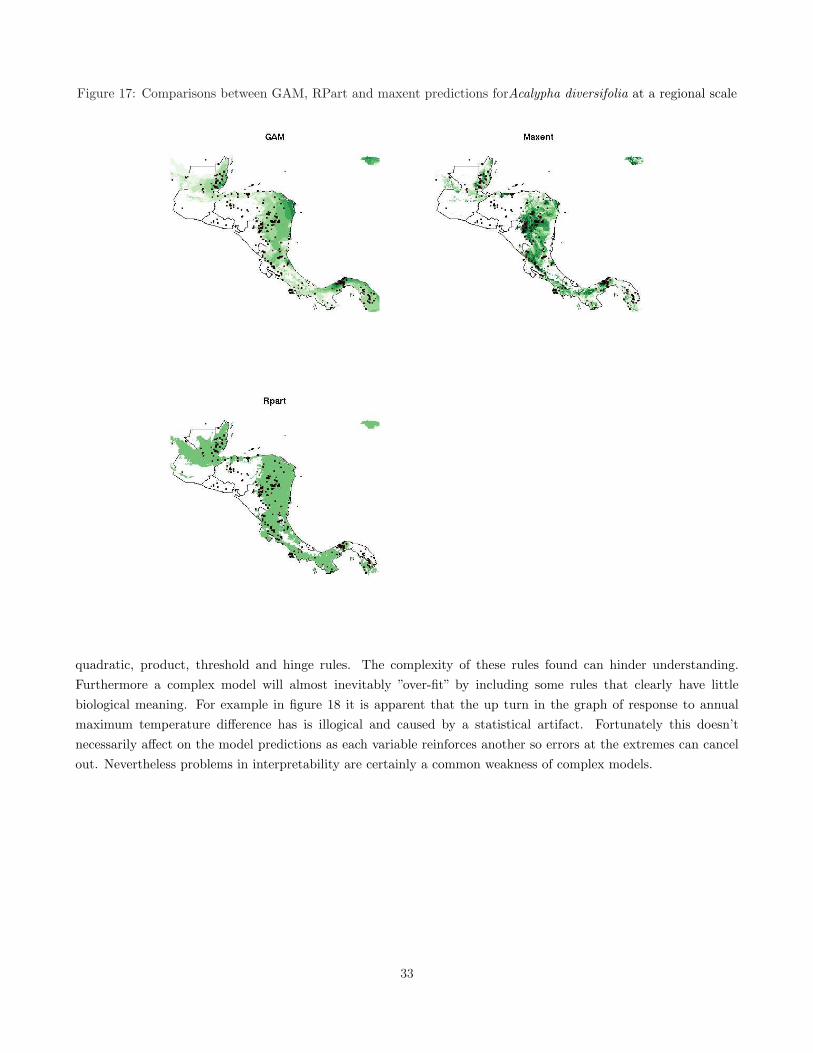
Figure 17: Comparisons between GAM, RPart and maxent predictions forAcalypha diversifolia at a regional scale

quadratic, product, threshold and hinge rules. The complexity of these rules found can hinder understanding.Furthermore a complex model will almost inevitably ”over-fit” by including some rules that clearly have littlebiological meaning. For example in figure 18 it is apparent that the up turn in the graph of response to annualmaximum temperature difference has is illogical and caused by a statistical artifact. Fortunately this doesn’tnecessarily affect on the model predictions as each variable reinforces another so errors at the extremes can cancelout. Nevertheless problems in interpretability are certainly a common weakness of complex models.

33

Figure 18: Maxent response curves for each of the variables used in predicting the distribution of Acalypha diversi-folia

GAMs can have similar undesirable properties. For example the model we fitted can be visualized using:

par(mfcol=c(4,2))

plot(mod1)

Figure 19: GAM response curves for each of the variables used in predicting the distribution of Acalypha diversifolia

19

The results for the GAM shown in figure 19 suffer from some of the same defects as the maxent models. GAMscan be forced to take simpler shapes by reducing the number of degrees of freedom used for the smoothing parameter.If terms are added in R such as s(tmax1,2) they reduce the smoothed curve to what is effectively a quadratic form.Again in the case of GAMs the additive nature of the model results in terms canceling out. The model predictions

34

are not necessarily seriously affected by clearly erroneous elements such as the rising trend of the curve with respectto daily temperature differences. These large differences are outside the range predicted for the species by the otherterms and are an another artifact of the form used for the curve.

Although the spatial predictions of rpart models tend to suffer from overly sharp cut off points due to the rulebased nature of the model, they have a very clear advantage in terms of interpretability. This is enhanced if lowcomplexity parameters are used for fitting. Figure 20 is easy to interpret. At each branching point read of the ruleand take the branch to the left to follow it. The leaf shows the proportion of occurrences (out of the total dataset that includes 5000 pseudo absences) with the eventual combination of rules. Thus we can conclude that morethan six months with precipitation of over 100 mm seem to be a condition for the presence of Acalypha diversifolia.Within the region with this property it is more likely to occur if the annual range of maximum temperature is below5.7 C. Again at the extreme tips of the branches the model suffers from slight over-fitting, but this can be ignored.Acalypha diversifolia is clearly a species that prefers moist tropical conditions.

Figure 20: Rpart classification tree for Acalypha diversifolia

It is possible to visualize model results easily in Google Earth using a small customized R script that can bepasted into the console.

toGE<-function(Gr=d,Layer=1,pal,nm="test.kml",imagenm="image1.png"){

png(imagenm,bg=’transparent’)

par(mar=c(0,0,0,0))

a<-Gr[[Layer]]

dim(a)<-c(Gr@grid@cells.dim[1],Gr@grid@cells.dim[2])

35

a<-a[,Gr@grid@cells.dim[2]:1]

image(a,col=pal)

dev.off()

X<-t(Gr@bbox)

X<-as.data.frame(X)

names(X)<-c("x","y")

coordinates(X)<-c("x","y")

X@proj4string<-Gr@proj4string

X<-spTransform(X,CRS("+proj=longlat +datum=WGS84"))

X<-as.data.frame(X)

N<-X[2,2]

S<-X[1,2]

E<-X[2,1]

W<-X[1,1]

fl<-imagenm

kmlheader<-c("<?xml version=’1.0’ encoding=’UTF-8’?>","<kml

xmlns=’http://earth.google.com/kml/2.0’>","<GroundOverlay>")

kmname<-paste("<name>",nm,"</name>",sep="")

icon<-paste("<Icon><href>",fl,"</href><viewBoundScale>0.75</viewBoundScale>

</Icon>",sep="")

latlonbox<-paste("<LatLonBox><north>",N,"</north><south>"

,S,"</south><east>",E,"</east><west>",W,"</west></LatLonBox>",sep="")

footer<-"</GroundOverlay></kml>"

x<-(kmlheader)

x<-append(x,kmname)

x<-append(x,icon)

x<-append(x,latlonbox)

x<-append(x,footer)

write.table(x,nm,quote=F,append=F,col.name=F,row.name=F)

}

After this function has been made available the kml file visualized in figure 21can be produced by typing:

fullgrid(preds)<-T

toGE(preds,3,pal=brewer.pal(7,"Greens"),"Acalypha_diversifolia.kml","maxent.png")

36

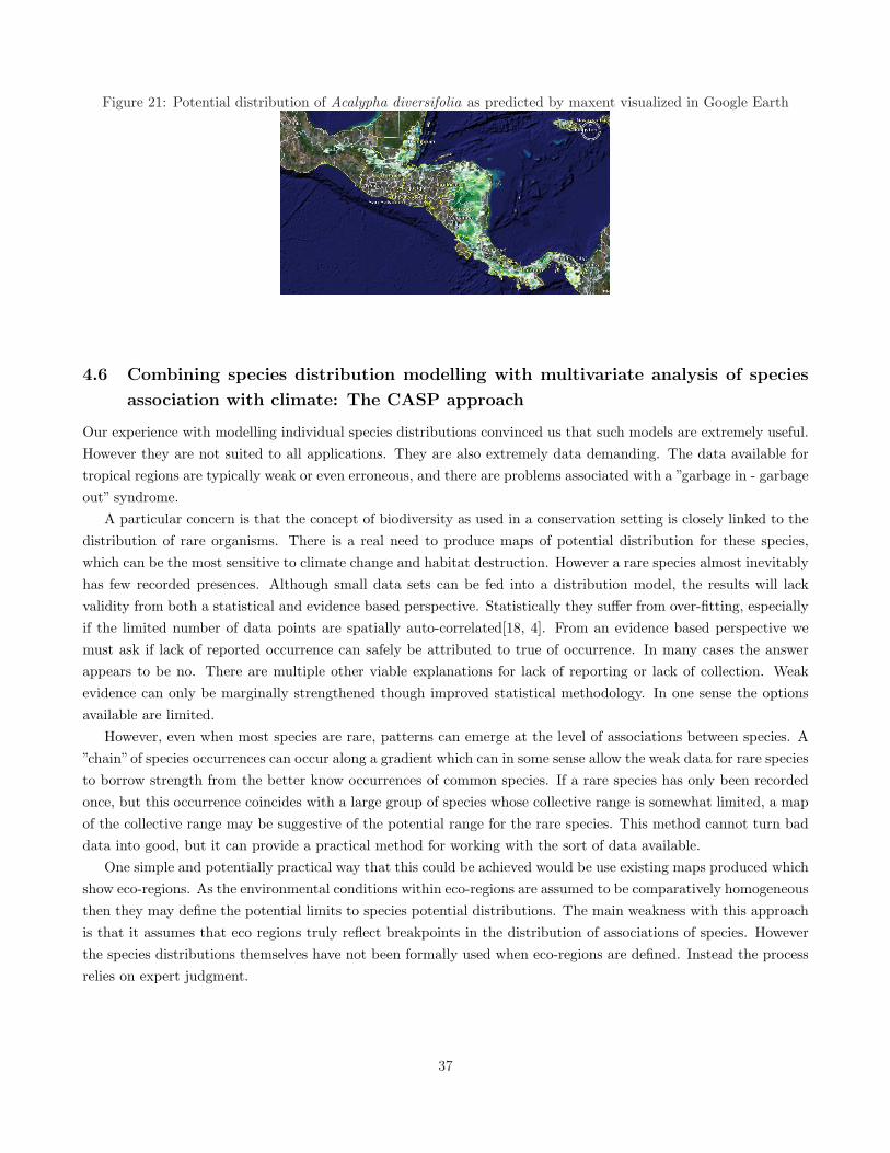
Figure 21: Potential distribution of Acalypha diversifolia as predicted by maxent visualized in Google Earth

4.6 Combining species distribution modelling with multivariate analysis of species

association with climate: The CASP approach

Our experience with modelling individual species distributions convinced us that such models are extremely useful.However they are not suited to all applications. They are also extremely data demanding. The data available fortropical regions are typically weak or even erroneous, and there are problems associated with a ”garbage in - garbageout” syndrome.

A particular concern is that the concept of biodiversity as used in a conservation setting is closely linked to thedistribution of rare organisms. There is a real need to produce maps of potential distribution for these species,which can be the most sensitive to climate change and habitat destruction. However a rare species almost inevitablyhas few recorded presences. Although small data sets can be fed into a distribution model, the results will lackvalidity from both a statistical and evidence based perspective. Statistically they suffer from over-fitting, especiallyif the limited number of data points are spatially auto-correlated[18, 4]. From an evidence based perspective wemust ask if lack of reported occurrence can safely be attributed to true of occurrence. In many cases the answerappears to be no. There are multiple other viable explanations for lack of reporting or lack of collection. Weakevidence can only be marginally strengthened though improved statistical methodology. In one sense the optionsavailable are limited.

However, even when most species are rare, patterns can emerge at the level of associations between species. A”chain”of species occurrences can occur along a gradient which can in some sense allow the weak data for rare speciesto borrow strength from the better know occurrences of common species. If a rare species has only been recordedonce, but this occurrence coincides with a large group of species whose collective range is somewhat limited, a mapof the collective range may be suggestive of the potential range for the rare species. This method cannot turn baddata into good, but it can provide a practical method for working with the sort of data available.

One simple and potentially practical way that this could be achieved would be use existing maps produced whichshow eco-regions. As the environmental conditions within eco-regions are assumed to be comparatively homogeneousthen they may define the potential limits to species potential distributions. The main weakness with this approachis that it assumes that eco regions truly reflect breakpoints in the distribution of associations of species. Howeverthe species distributions themselves have not been formally used when eco-regions are defined. Instead the processrelies on expert judgment.

37

Although we do not discount the value of eco-regions, we have been interested in finding methods that allow thedata on species distributions themselves to define them. This led us to combine methods used in community ecologywith those used by bio-geographers. Because of the extensive scale at which these models are applied we use theterm ”Climatically Associated Species Pools” [7]to describe the resulting groupings, rather than communities.[6]

The first step in the process is to divide the space to be modelled into what we might term ”pseudoquadrats”.The size of the quadrats will determine the number of co-occurring species found. There is a trade off here. Whilethe method requires all the quadrats which will be used to have more than 4-5 species, large quadrats will allowfor too much heterogeneity in climate within them[10]. This is a particular problem in mountainous areas withabrupt topography. For example the large quadrats shown in figure 22 illustrate the concept, but we would use afiner grain for modelling. In fact many collection points have multiple collections recorded from exactly the samecoordinates, so the aim of finding species that co-occur can be met with quite a fine grid.

Figure 22: Overlaying large (10’) quadrats on a the collection data for Nicaragua.

We have broken the R code used to produce CASPS into blocks. The first block that places the species intoquadrats is slightly involved, but the reader does not have to follow the details to use it. Note that decisionpoints have been marked in green and code that is specific to a particular computer in red. The object ”SMesoCli-maSPD.rob” contains a subset of the ”clima2” data set derived earlier.

library(spgrass6)

library(vegan)

library(mda)

library(mapdata)

setwd("/home/duncan/SpeciesModels/RData/CASP")

load("SMesoClimaSPD.rob" )

d<-read.table("SMesoTrees.txt",header=T)

38

#Decide on the size for the grid in degrees

###############

gridsize<-0.05 #

###############

#Set up an xseq using the limits for the overlay layers

xseq<-seq(clima2@bbox[1,1],clima2@bbox[1,2],by=gridsize)

#cut up the coordinates according to the sequence

gridlong<-as.numeric(cut(d$x,xseq))

#Turn the cut levels into x coordinate

gridlong<-clima2@grid@cellcentre.offset[1]+gridlong*gridsize

#Repeat the procedure for ys

yseq<-seq(clima2@bbox[2,1],clima2@bbox[2,2],by=gridsize)

gridlat<-as.numeric(cut(d$y,yseq))

gridlat<-clima2@grid@cellcentre.offset[2]+gridlat*gridsize

gridded.sp<-data.frame(x=gridlong,y=gridlat,sp=d$Name)

gridded.sp<-na.omit(gridded.sp)

coordinates(gridded.sp)<-c("x","y")

gridded.sp<-gridded.sp[!is.na(overlay(clima2,gridded.sp)),]

image(clima2,1,col=terrain.colors(100))

points(gridded.sp)

#Now set up the gridded.sp object as a data frame with cell codes

gridded.sp<-data.frame(x=gridded.sp@coords[,1],

y=gridded.sp@coords[,2],

code=paste(gridded.sp@coords[,1],gridded.sp@coords[,2],sep=" ")

,sp=gridded.sp[["sp"]])

str(gridded.sp)

#End of step 1.

#We now have a set of species referenced to grid cells, with all those falling

#Outside the mapped study region removed.

#This is passed on to step 2.

The next step in the analysis involves deciding which of the quadrats to use. Multivariate analysis breaks down(giving eigenvalues of one) if there are complete disjunctions between sets of species. It is also impossible to analyzedata that contains quadrats with only one occurrence. Thus after forming a vegetation matrix of species on siteswe remove the species with less than n occurrences and sites with less than j species. We can set n to 50 and j to 5in this example. We point out that this does not mean that we will completely ignore rarer species in the analysis.They are added back in the final stage. However they are not useful for defining the key relationships betweenspecies groups and climate.

#A key move is to set up a vegetation matrix (sp by sites) for vegan analysis

vegtable<-table(gridded.sp$code,gridded.sp$sp)

#But it is necessary to clean out very rare species and

#quadrats with insufficient species occurrences.

39

#####################

min.occurrences<-50 #

min.nsp<-5 #

#####################

f<-function(x)sum(x>0)

vegtable<-vegtable[,apply(vegtable,2,f)>min.occurrences]

vegtable<-vegtable[apply(vegtable,1,sum)>min.nsp,]

#A trick to get the coordinates of the cells back from the row names

# of the table.

coords<-do.call("rbind",strsplit(row.names(vegtable),split=" "))

coords<-data.frame(x=as.numeric(coords[,1]),y=as.numeric(coords[,2]))

cells<-data.frame(coords,ncollects=log2(apply(vegtable,1,sum)))

coordinates(cells)<-c("x","y")

Now we can carry out multivariate analysis using the R package vegan[21]. In this example we use canonicalcorrespondence analysis using all the seven climate layers. Sites are then grouped using k means clustering on theordination axis and colour coded. We have plotted two of the main climate variables (tmax6 and prec1) as contourson the diagram shown in figure 23.

#This is the ordination and k means clustering step

#There are a lot of important decisions here that require some understanding

#of the method in order to implement effectively.

#A simple choice is how many groups.

########

k<-8 #

########

env<-clima2@data[overlay(clima2,cells),]

vegtable<-as.data.frame(vegtable[apply(env,1,function(x)!any(is.na(x))),])

cells<-cells[apply(env,1,function(x)!any(is.na(x))),]

env<-env[apply(env,1,function(x)!any(is.na(x))),]

cca1<-cca(vegtable~.,env)

site.scores<-scores(cca1,display="sites",c(1:2))

set.seed(1)

cells[["kgroups"]]<-as.factor(kmeans(site.scores,k)$cluster)

plot(site.scores[,1],site.scores[,2],

xlab="First CCA axis", ylab="Second CCA axis",

main="",cex=0.8,col=as.numeric(cells[["kgroups"]]))

ordisurf(cca1, env[,1],main="",col="red",add=T)

ordisurf(cca1, env[,3], xlab="", ylab="",col="blue",lty=2,add=T)

40

Figure 23: Ordination diagram for CCA with climatic contours (tmax6 and prec1)

Once the ordination and k means clustering have been carried out the groups are treated as if they were species andtheir distribution mapped. However because the distribution of groups (Climatically Associated Species Pools) ismutually exclusive discriminant analysis is a suitable method for prediction. To avoid misunderstandings we stressthat it is the distribution of the lists of species, not the distribution of a given species that is mutually exclusive. Acommon species could be found in all the CASPs.

#The discriminant analysis phase.

pred.mod<-mda(cells[["kgroups"]]~.,data=env)

#Set up the spatial pixels predictors......

#...and predict onto the map.

clima2[["grps"]]<-as.numeric(predict(pred.mod,newdata=clima2@data))

image(clima2,"grps",col=1:8)

map("worldHires",c("mexico","Costa Ri","Panama","El Sal-

vad","Hondur","Nicara","Guate","Beliz"),add=T)

box()

axis(1)

axis(2)

grid()

41

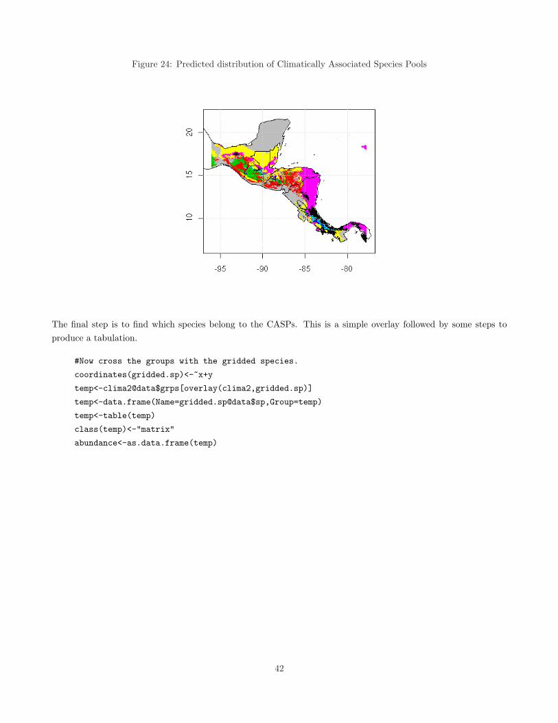
Figure 24: Predicted distribution of Climatically Associated Species Pools

The final step is to find which species belong to the CASPs. This is a simple overlay followed by some steps toproduce a tabulation.

#Now cross the groups with the gridded species.

coordinates(gridded.sp)<-~x+y

temp<-clima2@data$grps[overlay(clima2,gridded.sp)]

temp<-data.frame(Name=gridded.sp@data$sp,Group=temp)

temp<-table(temp)

class(temp)<-"matrix"

abundance<-as.data.frame(temp)

42

Figure 25: Part of the table of abundances of collections of species within the area of each CASP

Once the species pools have been defined in this way there are many possibilities for further analysis. They canbe used to produce potential distribution maps for each species by giving stronger colours to CASPS in which aspecies is more abundant.

q<-abundance[grep("Acalypha_d",row.names(abundance)),]

q<-as.vector(unlist(q))

clima2[["temp"]]<-q[clima2@data$grps]

image(clima2,"temp",col=c("white",brewer.pal(7,"Greens")))

map("worldHires",c("mexico","Costa Ri","Panama","El Sal-

vad","Hondur","Nicara","Guate","Beliz"),add=T)

axis(1)

axis(2)

box()

grid()

43

Figure 26: Predicted potential distribution forAcalypha diversifolia based on occurences within CASPS

Note that the predicted distribution for this species shown in figure 26using this methodology is very similar to thatsuggested by modelling at the individual species level. We have found that this correspondence between results isgeneral. However poor data leads to artifacts whatever approach is used.

Another simple but interesting analysis is to count the number of species occurring in each CASP as a simplemeasure of species richness. A variation on the theme is to only include species with more than n occurrences inorder to reduce bias through errors in georeferencing or determination.

f<-function(x)sum(x>4)

div<-apply(abundance,2,f)

clima2[["temp"]]<-div[clima2@data$grps]

image(clima2,"temp",col=c("white",brewer.pal(7,"Greens")))

map("worldHires",c("mexico","Costa Ri","Panama","El Sal-

vad","Hondur","Nicara","Guate","Beliz"),add=T)

axis(1)

axis(2)

box()

grid()

#Number of species with more than four occurences in each CASP

div

1 2 3 4 5 6 7 8

1094 552 388 154 432 993 869 664

44

Figure 27: Species richness as suggested by CASP analysis

The result of this shown in figure 27 confirms the fact that woody plant (regional or gamma) diversity is generallyhighest in the warm moist tropics and lower in drier cooler areas. One of the most useful outcomes of the analysisis that this observation is clearly linked to the underlying data and although some inevitable errors remain, at arather coarse scale potential distributions can be suggested for most species in the data base.

5 Modelling climate change scenarios

5.1 Extracting WMO GRIB formatted data

Data from a number of global circulation models parametrized for IPCC scenarios are available fromhttp://www.mad.zmaw.de/IPCC DDC/html/SRES AR4/index.html.Although this page mentions that data are available in ascii format, this does not mean the ascii grids that

are used in GIS. Output from climate models and large historical climatic data are usually held in either GRIB ornetCDF format. These formats have been specifically designed by the WMO (World Meteorological Organization)for efficient, compact storage of huge volumes of information. At the time of writing, as far as we know, theseformats are not directly readable either by any GIS or statistical software in general use. Research groups thatwork on climate modelling and monitoring have developed their own specialized tools for handling data in theseformats. It is therefore essential to obtain, install and learn to use these tools in order to have full access to thisessential source of input for species distribution modelling. Although tools for working with GRIB and netCDFhave not been designed with ”user friendly” GUIs, they do fit easily into the scripting framework that we use inthis document. At the time of writing the tool that appears to have the best documentation, ease of to installationand general simplicity of use is CDO (Climate Data Operators). The program can be downloaded as source codefrom http://www.mpimet.mpg.de/fileadmin/software/cdo/. This software offers a very strait-forward, powerfulcommand line interface that can be used for a large number of pre-processing and processing tasks. In this document

45

we use CDO to extract data in a usable form for further work in R and GRASS.

5.2 Installing CDO

We do point out that it is possible to build CDO under Cygwin within a Windows environment if this is necessary.It is a complicated procedure. As with all UNIX based tools installation is a much simpler process on a machinerunning some form of Linux. We have found that CDO builds from source cleanly under Ubuntu 7.04. The stepsused to install CDO are typical for any program that is distributed as source code. Using Konsole cd to the directorycontaining the package’s source code and type

sudo ./configure

to configure the package for your system. Then type

make

to compile the package. Finally

make install

to install the programs and any data files and documentation. Now in a console typing

cdo

should produce output detailing the operators available if CDO installed correctly. If you get output then CDO isinstalled and ready for use. Notice that although CDO is an extremely powerful program with a large number ofoperators, it does not have a graphical user interface or any form of directly visualizing output in the form of maps.This is irrelevant for our purposes as we use GRASS and R to achieve the visualization.

5.3 Obtaining the data

The data from the GCM scenarios can be download from the CERA portal http://cera-www.dkrz.de/ after regis-tering. As processing output from a GCM is a moderately time consuming affair, an initial challenge is choosingwhich output is most suitable from the large number of possibilities on offer. We have previously based our modelslargely on HADCM3 scenarios. At the time of writing HADCM3 output is not available for all the IPCC AR4 A1story line. There are outputs for the A2 and B2 scenarios and we will use these in this document. We will use thefollowing files derived from the A2 and B2 story-lines that are compatible with the methods used for processingWorldClim data.

HADCM3_A2_prec_1-1800.grb

HADCM3_A2_tmin_1-1800.grb

HADCM3_A2_tmax_1-1800.grb

HADCM3_B2_tmax_1-1800.grb

HADCM3_B2_prec_1-1800.grb

HADCM3_B2_tmin_1-1800.grb

46

One the files are downloaded into a suitable directory CDO can be used to provide information on the data storedwithin these files. For example:

cdo griddes HADCM3_A2_tmin_1-1800.grb

gridtype : lonlat

gridsize : 7008

xname : lon

xlongname : longitude

xunits : degrees_east

yname : lat

ylongname : latitude

yunits : degrees_north

xsize : 96

ysize : 73

xfirst : 0

xinc : 3.75

yfirst : 90

yinc : -2.5

Or typing:

cdo info HADCM3_B2_tmax_1-1800.grb

which produces a lot of output on the information provided for each of the set of grids in the file. From this outputit should be clear that each file contains 180 grids, one for each month between January 1950 and December 2099.The first set of results are climate data and the later results are model output.

5.4 Extracting fifty year monthly means

Our simulated data should be consistent with the data incorporated in the models we used for current distributionpredictions. WordClim monthly means are derived from fifty years of climate data. It is therfore appropriate touse fifty year blocks of modelled data and find the mean monthly values. We will use two commands in cdo to dothis. The first (splitsel) splits the data into blocks of fifty years and the second (ymonmean) calculates the monthlymeans over the years held in each of the files. Notice that a temporary file is produced for each split and thenremoved at the end of the process. As an aside, it should be clear from this small example that CDO is a fastefficient tool for data processing of great value to professional climatologists working on a daily basis with data ofthis complexity.

cdo splitsel,600 HADCM3_A2_tmin_1-1800.grb tmp1

cdo splitsel,600 HADCM3_A2_tmax_1-1800.grb tmp2

cdo splitsel,600 HADCM3_A2_prec_1-1800.grb tmp3

for i in $(seq 0 2)

do

cdo ymonmean tmp100$i.grb HADCM3_A2_tmin_50_$i.grb

47

cdo ymonmean tmp200$i.grb HADCM3_A2_tmax_50_$i.grb

cdo ymonmean tmp300$i.grb HADCM3_A2_prec_50_$i.grb

done

rm tmp*

If you now investigate the results using cdo info you will see that each file holds twelve global grids with the fiftyyear mean monthly values for the appropriate variable. We can reduce the data layers to two future scenarios foreach variable by subtracting the first fifty years data from each of the subsequent periods. This gives us a setof layers showing the expected mean change under the model scenarios. These layers are thus ready for a simpledownscaling procedure achieved by by adding the results to the much finer resolution WorlClim layers. Again weuse a small loop in a shell script to reduce typing slightly.

for i in $(seq 1 2)

do

cdo sub HADCM3_A2_prec_50_$i.grb HADCM3_A2_prec_50_0.grb HADCM3_A2_prec_dif_$i.grb

cdo sub HADCM3_A2_tmin_50_$i.grb HADCM3_A2_tmin_50_0.grb HADCM3_A2_tmin_dif_$i.grb

cdo sub HADCM3_A2_tmax_50_$i.grb HADCM3_A2_tmax_50_0.grb HADCM3_A2_tmax_dif_$i.grb

done

So now, by this stage, we have six files holding the mean change in each of prec, tmin and tmax for the next 50 and100 years under these climate change scenarios.

We can now form a directory for holding the results as ascii matrices and export the numbers held in the gridsas strait ascii.

mkdir ascii

cdo splitmon HADCM3_A2_prec_dif_1.grb temp1

cdo splitmon HADCM3_A2_tmin_dif_1.grb temp2

cdo splitmon HADCM3_A2_tmax_dif_1.grb temp3

cdo splitmon HADCM3_A2_prec_dif_2.grb temp4

cdo splitmon HADCM3_A2_tmin_dif_2.grb temp5

cdo splitmon HADCM3_A2_tmax_dif_2.grb temp6

for i in $(seq 1 9)

do

cdo output temp10$i.grb >ascii/prec50_$i.asc

cdo output temp20$i.grb >ascii/tmin50_$i.asc

cdo output temp30$i.grb >ascii/tmax50_$i.asc

cdo output temp40$i.grb >ascii/prec100_$i.asc

cdo output temp50$i.grb >ascii/tmin100_$i.asc

cdo output temp60$i.grb >ascii/tmax100_$i.asc

done

for i in $(seq 10 12)

do

cdo output temp1$i.grb >ascii/prec50_$i.asc

48

cdo output temp2$i.grb >ascii/tmin50_$i.asc

cdo output temp3$i.grb >ascii/tmax50_$i.asc

cdo output temp4$i.grb >ascii/prec100_$i.asc

cdo output temp5$i.grb >ascii/tmin100_$i.asc

cdo output temp6$i.grb >ascii/tmax100_$i.asc

done

rm temp*

The cdo command ”output” sends the results to stdout, which are then sent to the files using the redirect operator>. This results in a set of files with the raw numbers, but they do not have any information on the format. Weneed to add a header to each before they can be read into GRASS. In any suitable text editor write a simple filethat will form the header for all the ascii grids with the following form.

north: 90

south: -90

east: 0

west: -360

cols: 96

rows: 73

Make sure you include a carriage return on the last line. Save the file with the name ”header” in the ascii directory.Now we can use the concatenate command in the bash shell to add this header to all the previously built files. Asreassigning to an existing file is not allowed, we produce a new set of files and remove the previous files.

for i in $(seq 1 12)

do

cat ascii/header ascii/prec50_$i.asc>ascii/prec50h_$i.asc

cat ascii/header ascii/tmin50_$i.asc>ascii/tmin50h_$i.asc

cat ascii/header ascii/tmax50_$i.asc>ascii/tmax50h_$i.asc

cat ascii/header ascii/prec100_$i.asc>ascii/prec100h_$i.asc

cat ascii/header ascii/tmin100_$i.asc>ascii/tmin100h_$i.asc

cat ascii/header ascii/tmax100_$i.asc>ascii/tmax100h_$i.asc

rm ascii/prec50_$i.asc

rm ascii/tmin50_$i.asc

rm ascii/tmax50_$i.asc

rm ascii/prec100_$i.asc

rm ascii/tmin100_$i.asc

rm ascii/tmax100_$i.asc

done

5.5 Exporting to GRASS and visualising the data

The next step is to import all these files into GRASS. We use the same ”GLOBAL”location that holds the WorldClimdata, but it is a good idea to start a new mapset for this data. Lets call it HADCM3. After forming the mapset

49

in the GLOBAL location the startup screen should look something like figure 28, although in this case there are afew additional mapsets that have been set up for other purposes.

Figure 28: Startup screen for GRASS showing mapsets for scenario data.

Now once in GRASS cd 12to the directory where the ascii grids were stored

for i in $(seq 1 12)

do

r.in.ascii input=tmax100h_$i.asc output=tmax100.$i

r.in.ascii input=tmin100h_$i.asc output=tmin100.$i

r.in.ascii input=prec100h_$i.asc output=prec100.$i

r.in.ascii input=tmax50h_$i.asc output=tmax50.$i

r.in.ascii input=tmin50h_$i.asc output=tmin50.$i

r.in.ascii input=prec50h_$i.asc output=prec50.$i

done

This should result in a complete set of the very coarse resolution global circulation model results to be availableas GRASS raster layers. The default colour scheme is not suitable, so we can reassign colour rules to all thetemperature layers with:

for i in $(seq 1 12)

do

r.colors map=tmax100.$i rules=byr

r.colors map=tmin100.$i rules=byr

r.colors map=tmax50.$i rules=byr

r.colors map=tmin50.$i rules=byr

r.colors map=prec50.$i rules=ryg

12The term ”cd” is commonly used to mean change directory using the cd command. In this document a degree of working knowledgeof bash shell commands is assumed.

50

r.colors map=prec100.$i rules=ryg

done

Now if you have previously imported a vector layer showing country boundaries into the location the map shownin figure 30 can be produced by

d.mon start=x

d.mon select=x0

d.rast.leg tmax100.1

d.vect country type=boundary

Figure 29: Predicted change in mean January maximum temperature in the period 2050-2099 compared with1950-1999 (HADCM3 A2)

There are several points to note from figure 29. The A2 scenario is among the most alarming of the IPCC storylines, so models using the carbon emissions from this scenario show quite dramatic global change. Winter warmingis mainly concentrated in the arctic seas. The very extreme value of an 18.1 C increase is attributable to a singlepixel, which tends to exaggerate the scale. A rather better visual presentation of the results would truncate someof the values as is done by the on-line results server http://www.ipcc-data.org/cgi-bin/ddcvis/gcmcf. 13The sameslight exaggeration of the results is found in figure 29.

13It is quite possible to download ascii values directly from this map server, which is a potentially simpler, although much less flexiblealternative to extracting values from GRIB data sets. However not all AR4 scenarios are yet available from this source at the time ofwriting.

51

Figure 30: Predicted change in mean May maximum temperature in the period 2050-2099 compared with 1950-1999(HADCM3 A2)

5.6 Downscaling the data

The next step in processing the data is downscaling.There are a number of challenges associated with downscaling from the extremely coarse resolution of the

global circulation models to the 1-10 km grids used for regional species distribution modelling. These add to theuncertainties inherent in the modelling exercise. For example, differences in predicted rainfall for future scenariosare measured in mm per day over the month of interest. Because the climate data used as a baseline for the GCMsis coarse it is quite possible at a local scale to find that simply adding the change over the surface can lead topredictions of negative rainfall.

The simplest option for temperature would appear to be to add the WorldClim and GLM surfaces together.The script below will do this for previously imported tmax layers for the 100 years scenario. In order to runthe script it would be convenient to move into a new mapset for the output with access (use g.mapsets) bothto the PERMANENT mapset with the original WorldClim data as imported in the first part of this report andthe HADCM3 scenario data as imported in this report. Make sure the resolution of the region is set to g.regionres=00:03 for approximately 5km grid square output.

for i in $(seq 1 12)

do

r.to.vect tmax100.$i

r.mapcalc "tmax100.d$i=tmax100.$i+tmax$i/10"

done

However this approach results in very obvious artifacts with some of the underlying divisions between cells at thecoarse resolution very obvious in the output as shown in figure 31.

52

Figure 31: Artifacts due to large grain of GCM models when simple additive downscaling is used.

A partial solution to the ”ghost” of the coarse scale model results is to first smooth between the centres of thecoarse grid squares before adding in the results. The code below will do this for all the output of the ”100” yearsimulation.

for i in $(seq 1 12)

do

g.region res=03:00

r.to.vect -z input=prec100.$i feature=point output=temp1

g.region res=00:03

v.surf.idw input=temp1 output=temp1 layer=0

r.mapcalc "prec100.s$i=if(temp1*30+prec$i>0,temp1*30+prec$i,0)"

g.mremove vect=temp* -f

g.mremove rast=temp* -f

done

for i in $(seq 1 12)

do

g.region res=03:00

r.to.vect -z input=tmax100.$i feature=point output=temp1

g.region res=00:03

v.surf.idw input=temp1 output=temp1 layer=0

r.mapcalc "tmax100.s$i=temp1+tmax$i/10"

g.mremove vect=temp* -f

g.mremove rast=temp* -f

done

for i in $(seq 1 12)

do

g.region res=03:00

r.to.vect -z input=tmin100.$i feature=point output=temp1

53

g.region res=00:03

v.surf.idw input=temp1 output=temp1 layer=0

r.mapcalc "tmin100.s$i=temp1+tmin$i/10"

g.mremove vect=temp* -f

g.mremove rast=temp* -f

done

Figure 32: Additive downscaling preceded by inverse distance weighting interpolation between the centre points ofeach GCM cell.

5.7 Moving the results to R for modelling

Now we can move the data into R as we did with the original climate data.

library(spgrass6)

a<-paste("tmax100.s",1:12,sep="")

a<-c(a,paste("tmin100.s",1:12,sep=""))

a<-c(a,paste("prec100.s",1:12,sep=""))

clima<-readRAST6(a)

The names can be changed so the object is identical to the original climate object.

a<-paste("tmax",1:12,sep="")

a<-c(a,paste("tmin",1:12,sep=""))

a<-c(a,paste("prec",1:12,sep=""))

names(clima@data)<-a

From now on we can substitute the new clima object in R where appropriate.

f<-function(x)max(x[1:12])-min(x[1:12])

clima[[”AnnualMaxTDif”]]<-apply(clima@data,1,f)

54

f<-function(x)max(x[1:12]-x[13:24])

clima[["DailyTDif"]]<-apply(clima@data,1,f)

f<-function(x)sum(x[25:36]>100)

clima[["GrowingMonths"]]<-apply(clima@data,1,f)

clima2<-clima

clima2@data<-clima2@data[,c(6,13,25,30,37,38,39)]

If you have followed the methodology to this point, substituting the new scenario climate data in R should be straitforward. The models are first fit by overlaying the original clima layers then the new layers are substituted whenusing the predict method. A future addition to this report will document in more detail how the scenario data canbe used to predict species turnover.

References

[1] Hansen, M., DeFries, R., Townshend, J.R.G., Sohlberg, R., Dimiceli, C., and Carroll, M., 2002, Towards noperational MODIS continuous field of percent tree cover algorithm: examples using AVHRR and MODISdata. (2002) Remote Sensing of the Environment 83, 303-319.

[2] Hansen, M., DeFries, R., Townshend, J.R.G., Carroll, M., Dimiceli, C., and Sohlberg, R., 2002, Global percenttree cover at a spatial resolution of 500 meters: first results of the MODIS vegetation continuous fields algorithm.submitted to Earth Interactions

[3] Hijmans, R.J., S.E. Cameron, J.L. Parra, P.G. Jones and A. Jarvis, 2005. Very high resolution interpolatedclimate surfaces for global land areas. International Journal of Climatology 25: 1965-1978. (pdf)

[4] Barry, S. & Elith, J. (2006) Error and uncertainty in habitat models. Journal of Applied Ecology, 43, 413-423.

[5] Elith, J., Graham, C.H., Anderson, R.P., Dudık, M., Ferrier, S., Guisan, A., Hijmans, R.J., Huettmann, F.,Leathwick, J.R., Lehmann, A., Li, J., Lohmann, L.G., Loiselle, B.A. Manion, G., Moritz, C., Nakamura, M.,Nakazawa, Y., Overton, J.M., Peterson, A.T., Phillips, S.J., Richardson, K.S., Scachetti-Pereira, R., Schapire,R.E., Soberon, J., Williams, S., Wisz, M.S. & Zimmermann, N.E. (2006) Novel methods improve prediction ofspecies’ distributions from occurrence data. Ecography, 29, 129-151.

[6] Ferrier, S. & Guisan, A. (2006) Spatial modelling of biodiversity at the community level. Journal of AppliedEcology, 43, 393-404.

[7] Golicher, D J, Cayuela L, J. Alkemade R J, Gonzalez-Espinosa M & Ramırez-Marcial N (2007) ApplyingClimatically Associated Species Pools to modeling compositional change in tropical montane forests (Acceptedfor publication in Global Ecology and Biogeography July 2007)

[8] Guisan, A. & Zimmermann, N.E. (2000) Predictive habitat distribution models in ecology. Ecological Modelling,135, 147-186.

[9] Guisan, A., Lehmann, A., Ferrier, S., Austin, M., Overton, J.MC.C., Aspinall, R. & Hastie, T. (2006) Makingbetter biogeographical predictions of species’ distributions. Journal of Applied Ecology, 43, 386-392.

55

[10] Guisan, A., Graham, C.H., Elith, J., Huettmann, F. & NCEAS Species Distribution Modelling Group. (2007)Sensitivity of predictive species distribution models to change in grain size. Diversity and Distributions, 13,332-340.

[11] Lennon, J.J., Kunin, W.E., Corne, S., Carver, S. & Van Hees, W.W.S. (2002) Are Alaskan trees found inlocally more favourable sites in marginal areas? Global Ecology and Biogeography, 11, 103-114.

[12] Luoto, M., Poyry, J., Heikkinen, R.K. & Saarinen, K. (2005) Uncertainty of bioclimate envelope models basedon the geographical distribution of species. Global Ecology and Biogeography, 14, 575-584.

[13] Pearson, R.G. & Dawson, T.P. (2003) Predicting the impacts of climate change on the distribution of species:are bioclimate envelope models useful? Global Ecology and Biogeography, 12, 361-371.

[14] Pearson, R.G. & Dawson, T.P. (2004) Bioclimate envelope models: what they detect and what they hide –response to Hampe (2004). Global Ecology and Biogeography, 13, 471-472.

[15] Pearce, J.L., Cherry, K., Drielsma, M., Ferrier, S. & Whish, G. (2001) Incorporating expert opinion andfine-scale vegetation mapping into statistical models of faunal distribution. Journal of Applied Ecology, 38,412-424.

[16] Phillips Steven J. , Robert P. Anderson, Robert E. Schapire. Maximum entropy modeling of species geographicdistributions. Ecological Modelling, 190:231-259, 2006.

[17] Thuiller, W., Araujo M.B., Lavorel S. (2003) Generalized Models versus Classification Tree Analysis: a com-parative study for predicting spatial distributions of plant species at different scales. Journal of VegetationScience 14, 669-680 PDF

[18] McPherson, J.M., Jetz, W. & Rogers, D.J. (2004) The effects of species’ range sizes on the accuracy of distri-bution models: ecological phenomenon or statistical artefact? Journal of Applied Ecology, 41, 811-823.

[19] Terry M Therneau and Beth Atkinson. R port by Brian Ripley <ripley@stats.ox.ac.uk>.(2006). rpart: Recursive Partitioning. R package version 3.1-33. S-PLUS 6.x original athttp://mayoresearch.mayo.edu/mayo/research/biostat/splusfunctions.cfm

[20] Trevor Hastie (2006). gam: Generalized Additive Models. R package version 0.98.

[21] Oksanen, J., Kindt, R., Legendre, P. & O’Hara, R.B. (2007). vegan: Community Ecology Package version1.8-6. http://cran.r-project.org/

[22] R Development Core Team (2007). R: A language and environment for statistical computing. R Foundationfor Statistical Computing, Vienna, Austria. ISBN 3-900051-07-0, URL http://www.R-project.org.

56