A Methodology for Architectural-Level Reliability Risk Analysis Sherif M. Yacoub, Hany H. Ammar1

Publishing Systems and Solutions Laboratory HP Laboratories Palo Alto HPL-2001-132 May 30th , 2001* E-mail: sherif_yacoub@hp.com, hammar@wvu.edu risk analysis, risk modeling, component-dependency graphs, software architecture, dynamic metrics

Risk assessment is an essential process of every software risk management plan. Several risk assessment techniques are based on the subjective judgement of domain experts. Subjective risk assessment techniques are human intensive and error-prone. Risk assessment should be based on product attributes that we can quantitatively measure using product metrics. This paper presents a methodology for reliability risk assessment at the early stages of the development lifecycle, namely the architecture level. We describe a heuristic risk assessment methodology that is based on dynamic metrics. The methodology uses dynamic complexity and dynamic coupling metrics to define complexity factors for the architecture elements (components and connectors). Severity analysis is performed using Failure Mode and Effect Analysis (FMEA) as applied to architecture models. We combine severity and complexity factors to develop heuristic risk factors for the architecture components and connectors. Based on analysis scenarios, we develop a risk assessment model that represents components, connectors, component risk factors, connector risk factors, and probabilities of component interactions. We also develop a risk analysis algorithm that aggregates risk factors of components and connectors to the architectural level. Using the risk aggregation and the risk analysis model, we show how to analyze the overall risk factor of the architecture as the function of the risk factors of its constituting components and connectors. A case study of a pacemaker architecture is used to illustrate the application of the methodology. The methodology is used to identify critical components and connectors and to investigate the sensitivity of the architecture risk factor to changes in the heuristic risk factors of the architecture elements.

* Internal Accession Date Only Approved for External Publication 1 Department of Computer Science and Electrical Engineering, West Virginia University, Morgantown, WV 26506-6109 To be published in IEEE Transactions on Software Engineering Copyright IEEE 2001

2

1 Introduction

The process of risk assessment is useful in identifying complex modules that require detailed inspection,

estimating potentially troublesome modules, and estimating testing effort. According to NASA-STD-

8719.13A [20] risk is a function of: the possible frequency of occurrence of an undesired event, the

potential severity of resulting consequences, and the uncertainties associated with the frequency and

severity. The STD-8719.13A standard [20] defines several types of risks, for example, availability risk,

acceptance risk, performance risk, cost risk, schedule risk, etc. In this study, we are concerned with

reliability-based risk , which depends on the probability that the software product will fail in the

operational environment and the adversity of that failure.

For the purpose of this work, we adopt the definition in [23], which defines risk as a combination of two

factors: probability of malfunctioning (failure) and the consequence of malfunctioning (severity). The

probability of failure depends on the probability of existence of a fault combined with the possibility of

exercising that fault. Whereas a fault is a feature of a system that precludes it from operating according to

its specification, a failure occurs if the actual output of the system for some input differs from the

expected output [36]. It is difficult to find exact estimates for the probability of failure of individual

components in the system. Therefore, in this study we use quantitative factors that have been proven to be

correlated with the probability of faults in the development of software components, such as complexity

factors [18]. Moreover, to account for the probability of a fault manifesting itself into a failure, we use

dynamic metrics. Dynamic metrics are used to measure the dynamic behavior of a system based on the

premise that active components are sources of failures [34]. A fault may not manifest itself into a failure

if never executed. Therefore, it is reasonable to use measurements obtained from executing the system

models to perform risk assessment and analysis1. To study the second factor in the risk definition, the

consequence of a failure (severity), we apply the MIL_STD 1629A Failure Mode and Effect Analysis [7].

Risk assessment can be performed at various development phases. Architecture models abstract design

and implementation details and describe the system using compositions of components and connectors. A

component can be as simple as an object, a class, or a procedure, and as elaborate as a package of classes

or procedures. Connectors can be as simple as procedure calls or as elaborate as client-server protocols,

links between distributed databases, or middlewares. We envisage that risk assessment at the architecture

level is more beneficial than assessment at later development phases. An early detection and correction of

problems is much less costly than detection at the code level. The architecture of a software is critical to

3

all development phases. If the architecture is very complex, then design and coding are likely to take

more time and produce more errors.

To conduct risk assessment at the architecture level, we use architecture models that we can simulate.

Using simulation models gives our risk assessment methodology two advantages:

• First, we are able to obtain measurement of the dynamic behavior of components and connectors

using dynamic metrics. These measures are used as dynamic complexity factors in developing risk

indices for individual components and connectors.

• Second, we are able to study the consequences of a failure and its effect (severity) by simulating the

architecture. Severity is the second factor used in developing risk indices for components and

connectors.

The additional effort of developing these simulation models should be minimized. Therefore, the same

architecture models developed by the system analyst during the system analysis phase should be used by

the risk assessment and analysis methodology.

1.1 Motivations

We are concerned with risk assessment and analysis for software architectures. This work is motivated by

the need to:

• Classify the system architecture elements according to their relative importance in terms of such factors

as severity and complexity and identify components with high risk factor, which could require more

development resources.

• Assess the system (subsystem) risk as an aggregate of individual component and connector risk factors.

In large hierarchical systems, a system is composed of several subsystems, which in turn are composed

of components and connectors. To classify subsystems according to risks, we need to develop

algorithms that aggregate risk factors of the subsystem constituents to the subsystem level and hence we

obtain and compare risk factors for subsystems.

• Develop automatable means to assess software product risks early in the development process. Risk

assessment techniques should be based on quantitative metrics that can be evaluated systematically with

little involvement of subjective measures from domain experts. Several tools enable us to obtain these

metrics early at the specification levels [21,24]. Metrics for risk assessment should provide

1 We note that it is not sufficient to draw general correlation between the measured complexity of execution structure (using dynamics metrics) and the probability of failure from one case study. Several empirical studies are required to support the correlation.

4

measurement quantities that integrate risk assessment models, risk management plans, and mitigation

strategies.

• Study the sensitivity of the application risk to variations in the risk factors of architecture components

and connectors. This could guide the process of identifying critical architecture elements and analyze

the effect of replacing components with new ones with improved quality, i.e. lower risk estimates.

1.2 Contributions

In this paper, we

• develop a new methodology to perform reliability risk assessment and reliability risk analysis at the

architecture level.

• describe a heuristic risk assessment technique that is based on dynamic metrics. Our methodology

uses dynamic complexity and dynamic coupling metrics, which we can obtain from simulating the

software architecture specifications. Severity analysis is performed using Failure Mode and Effect

Analysis (FMEA) with the aid of simulation runs to study the effect of a failure. We combine severity and

complexity factors to develop heuristic risk factors for the architecture components and connectors.

• develop a new risk analysis model and a risk analysis algorithm that aggregates risk factors of

components and connectors to the architecture level. We enhance Component Dependency Graphs

(CDGs) [33,35] for the purpose of risk assessment and develop a risk aggregation algorithm that traverses

the new graphs. Using the algorithm and the model, we show how to analyze the overall risk factor of the

architecture as the function of the risk factors of its components and connectors.

• apply the proposed risk assessment methodology to a case study of a pacemaker to identify critical

components and connectors.

This paper is organized as follows. Section 2 gives a short background on dynamic metrics and

component dependency graphs on which our methodology is based. Section 3 discusses the methodology

and its steps. Section 4 is an application of the methodology to the pacemaker case study. Section 5

summarizes the related work. Finally we conclude the paper and discuss future extensions.

2 Background

The work in this study is based on our earlier work on dynamic metrics and reliability modeling and

analysis of software architectures. We use dynamic metrics [34] in our risk assessment methodology to

develop complexity factors for architecture elements. We also enhance Component Dependency Graphs

(CDGs) [33,35] for the purpose of risk assessment and develop a risk aggregation algorithm that traverses

5

the new graphs. The following subsections give a quick overview on dynamic metrics and CDGs. For

further detailed the reader is referred to [33, 34, 35].

2.1 Dynamic Metrics

The complex dynamic behavior of many real-time applications motivates a shift in interest from

traditional static metrics to dynamic metrics. As components are invoked (executed), they become active

for specific duration of time performing the requested functionalities. The most active set of components

are sources of errors because they execute more frequently and experience numerous state changes.

Therefore there is a higher probability that if a fault exists in an active component, it will easily manifest

itself into a failure. For risk analysis at the architecture level, we are interested in the risks of a failure.

Hence, we are motivated to assess the complexity of components and connectors as expected at run-time

using dynamic metrics.

We perceive that, given advances in architecture modeling and simulation tools [21,24], we are able to

evaluate dynamic coupling and dynamic complexity from executable architectures. In [34], we define a

set of dynamic metrics for coupling and complexity, and we discuss the impact of these metrics on

software quality attributes such as maintainability, reusability, and error-proneness. We also show how to

use executable architecture models to obtain measurement for dynamic coupling and dynamic

complexity. The dynamic coupling metric measures how active a link between two components (the

connector) is during the execution of a particular scenario. This measure can then be prorated with the

scenario profile to obtain a measure for connector complexity. The dynamic complexity metric measures

the complexity of the dynamic behavior of a particular component in a given scenario. This measure can

then be prorated with the scenario profile to obtain a measure for component complexity.

In this study, we use the dynamic metrics defined in [34] to obtain complexity factors for each

architecture element. A complexity factor for each component is obtained using the dynamic complexity

metric for the behavioral specification of that component. A complexity factor for each connector is

obtained using the dynamic coupling metric for the messaging protocol of that connector. Both dynamic

coupling and dynamic complexity metrics are discussed as part of the complexity analysis step of the

proposed methodology (section 3.2).

2.2 Component Dependency Graphs

Component Dependency Graphs (CDGs) are introduced in [33] as probabilistic models for the purpose of

reliability analysis at the architecture level. These graphs are further extended to analyze the reliability of

distributed component-based systems [35]. A CDG is a reliability analysis model for component-based

systems that extends control flow graphs. It models a system as a composition of subsystems,

6

components, and connectors between components. CDGs are directed graphs that represent components,

component reliabilities, connectors, connector (links and interface) reliabilities, and transition

probabilities. CDGs are developed from scenarios. A scenario is a set of component interactions triggered

by specific input stimulus [31]. One way to model scenarios is using the Unified Modeling Language

(UML) [29] sequence diagrams . By using sequence diagrams, we are able to collect statistics required

for building CDGs, such as the average execution time of a component in a scenario, the average

execution time of a scenario, and possible interactions among components2. Scenarios are also related to

the concept of operations and run-types used for operational profiles [19] as discussed in [33]. Figure 1

illustrates a simple CDG example consisting of four components, C1, C2, C3, and C4.

A CDG is defined as follows:

CDG=<N,E,s,t>; where N is set of nodes, E is set of edges, and s and t are the start and termination

nodes, i.e. N = {n}, E ={e},

n = < Ci, RCi, ECi >; where Ci is the name of the ith component, RCi is component reliability, and ECi

is average execution time of a component Ci. ECi is given by equation 1:

where:

PSk : is the probability of execution of scenario Sk ,

|S|: is the total number of scenarios,

Time(Ci) is the execution time of Ci . Time(Ci) can be estimated as the sum of its active

time along its lifeline in a sequence diagram (for example, see the vertical rectangles

attached to the lifeline of components in the sequence diagrams in Appendix B),

Ci is said to be in Sk if it participates in the execution of scenario Sk.

e = <Tij, RTij, PTij>, where Tij is transition from node ni to nj in the graph, RTij is transition reliability,

PTij is transition probability. PTij is given by equation 2:

where:

2 For details about how to collect these parameters, we refer the reader to [33]

kii

S

kSCCTimePSEC ki in )(*

||

1∑

=

= Eq 1

Eq 2

kljili Nl

jiS

k SCCCCCInteractCCInteract

PSPT kij

in ,|),(||),(|

*,,..,1

||

1

=

==∑

and l<>i

7

|S| : is the number of scenarios,

PSk : is the probability of execution of scenario Sk ,

N : is the number of components in the application, and

|Interact(Ci,Cj)| : is the number of times Ci interacts with Cj in a given scenario Sk.

Our risk assessment methodology does not use RCi and RCij, instead risk factors for components and

connectors are used as explained later in section 3.4.

Figure 1 A sample CDG

Based on CDGs, an algorithm has been developed in [33] to analyze the reliability of the application and

study the sensitivity of the application reliability to variations in the reliabilities of components and

interfaces. In this study, we extend CDGs for the purpose of risk analysis. We use risk factors instead of

reliability estimates and we show how to calculate the CDG parameters from simulating the architecture

description of a system. We elaborate on CDGs in section 3.5 as part of the proposed risk assessment

methodology.

<C1,RC1=0.2, EC 1=3>

<T1 2,RT 12=1,PT12=0.8>

<C3,RC3=0.7,EC3=6><C2,RC2=0.4,EC2=4>

<C4,RC4=0.8, EC4=3>

<T13 ,RT 13=1,PT13= 0.2>

<T 24,RT24=1,PT24=1><T 34 ,RT3 4=0.9,PT 34=1>

s

<T43 ,RT43=1,PT43=0.7>

t

PT4 ,t=0.3

8

3 The Risk Assessment Methodology

The proposed methodology is defined by the following steps:

1. Modeling the system architecture using an ADL (section 3.1), 2. Performing complexity analysis using simulation (section 3.2), 3. Performing severity analysis using FMEA and simulation runs (section 3.3), 4. Developing heuristic risk factors for components and connectors (section 3.4), 5. Developing CDGs for risk assessment purposes (section 3.5), 6. Performing risk assessment and analysis using a graph traversal algorithm (section 3.6).

3.1 Architecture Modeling

Software development based on architectures shifts the focus towards architecture elements such as

components and connectors where connectors are treated as top-level constructs [28, 3]. Architecture

Description Languages (ADLs) [1,30] enable the formalization of the description of a software

architecture and hence enable the execution of some preliminary analysis to discover early stage problems

before the detailed design phase. The literature is plentiful of ADLs that we can use to specify the

architecture of a software system [17].

The dynamic behavior specifications of a software system describe how the system is expected to behave

at run time. Risks associated with system failures at run time can be studied by analyzing the dynamic

behavior of the system and of its individual components. Therefore, our risk analysis methodology is

mostly concerned with the dynamic specifications of the software system architecture, which can be

captured in terms of the interactions between components as well as behavior of individual components.

In our methodology, we require that the ADL provides support for modeling:

• The interactions between components.

• The behavior of individual components.

The former can be specified using sequence diagrams, which define the sequence of interaction between

components in a timely ordered manner. The latter can be specified using statecharts that define the

component’s states and how it responds to external stimuli according to its state. The Unified Modeling

Language (UML) [29] is becoming the de facto standard for modeling software systems. UML defines

modeling specifications that can be used to specify the dynamic aspects of an architecture. We use UML

statecharts diagrams to specify the individual component behavior and UML sequence diagrams to

specify interactions between components. However, UML does not specify how to simulate the

architecture models. To simulate UML specifications, the Real-Time Object-Oriented Modeling (ROOM)

9

[27] can be used. ROOM is an ADL that can be used to simulate statechart specifications of individual

components and sequence diagram specifications of component interactions.

Several tools are available to simulate ROOM and UML architecture descriptions [24, 21]. In this study,

we use the ObjecTime tool [21] to simulate the architecture, obtain dynamic measurements, and study

effect analysis. In the ROOM ADL, the architecture is specified using the component (actor) diagrams.

Each component is specified using a ROOMchart (the ROOM equivalence of Harel statechart [8]). Each

connector is specified as a protocol of message exchange between two components with ports indicating

which messages are input and which are output from the port. For details about the ROOM modeling

language we refer to [27]. The same study can be conducted using Rose Real-Time simulation

environment [24], which integrates a ROOM simulation capability into UML modeling environment.

3.2 Complexity Analysis

Traditionally we measure system reliability in terms of time between failures or number of faults found

during a specific period of time. Some empirical studies found a correlation between the number of faults

found in a software and the complexity of the system [18]. The more complex the system is, the higher

the probability that it will have faults. To improve software quality and develop risk mitigation strategies,

we should be able to predict early on in the development lifecycle those components that are likely to

have higher fault rates. Hence complexity metrics are used in our risk assessment technique. To

incorporate the fact that risk assessment should take in consideration the probability of exercising the

fault, we use dynamic metrics. In our study, we use dynamic complexity of statecharts and dynamic

coupling between components as dynamic metrics of architecture elements [34]. These metrics are

obtained at the specification level - statechart specification of components and scenarios of component

interactions- which are different from traditional code level metrics.

3.2.1 Component Complexity

Software complexity metrics have been used by scientists and engineers for a long time. In 1976, McCabe

introduced cyclomatic complexity measurement as an indicator for system quality in terms of testability

and maintainability. Cyclomatic complexity is based on program graphs and is defined in equation 3.

where: e=number of edges, n=number of nodes

In our study, we develop complexity factor for each component using the cyclomatic complexity of the

statechart specification [8] of a component. For each execution scenario, say Sk, a subset of the statechart

specification of the component is executed in terms of state entries, state exits, and fired transitions. This

subset of the statechart model contains segments of specification code required to fire transitions, send

Eq. 3VG=e-n+2

10

s21

s22

Iinit

initI

s11t11

t12t13

s1

s2

messages to other components, check condition and triggers, etc. Hence, we are able to aggregate the

cyclomatic complexity of the executed path for each component Ci for a scenario Sk. This measure is

called operational complexity [34] and is denoted as cpxk(Ci)

Sometimes, the large number of states in a statechart of a complex component can be reduced by breaking

these states into separate sub-machines and packaging them within composite states. A composite state is

composed of lower level states. In statecharts, transitions between composite states are cut into transition

segments. A transition segment is part of the transition that belongs to a composite state. Transition points

provide a basis for correlating different segments of the same transition. To estimate the cyclomatic

complexity of the transition between composite states we sum the cyclomatic complexity of all transition

segments, the exit code segment of the source node, and entry code segment of the destination node. For

example in Figure 2, VG for the transition from state s11 to s22 is VGx(s11) + VGa(t11) + VGx(s1)+

VGa(t12) + VGe(s1) + VGa(t13) +VGe(s22), where VGx is the complexity of the exit code segment, VGa is

the complexity of the action code segment, and VGe is the complexity of the entry code segment.

Figure 2 An example of a transition between composite states

To obtain the dynamic complexity metric from ROOM simulation models, we attribute the model with a

complexity variable for each component. For each execution scenario, these variables are updated with

the complexity measure of the thread of execution that is triggered for that particular scenario. At the end

of the simulation, the simulation tool reports the dynamic complexity value for each component. Using

the probabilities of scenarios (PSk), we calculate the average operational complexity measure for each

component as shown in equation 4.

where |S| is the number of scenarios.

We then obtain a normalized complexity measure for each component by dividing the complexity

measure of each component by the highest complexity value of all components in the architecture.

3.2.2 Connector Complexity

To assign complexity factors to architecture connectors we use dynamic coupling metrics. Dynamic

coupling metrics are defined in [34] as export dynamic coupling and import dynamic coupling. The

distinction between export and import coupling is mainly in the direction of data and control flow from/to

a component in the software architecture. Export coupling measures coupling as a component sends

Eq. 4∑=

×=||

1

)()(S

k

ikki CcpxPSCcpx

11

(export) messages or data to other components. Import coupling measures coupling as a component

receives (imports) messages or data from other components in the architecture.

For this case study, we use export dynamic coupling. Export coupling is used as opposed to import

coupling because the structure of the CDG model (section 3.5) as well as the risk analysis algorithm

(section 3.6) are mainly based of sequence of component interactions, i.e. one component invoking the

next. Export coupling accounts for the fact that an error in a currently executing component could be

exported to the called component (next in the execution list).

ECk(Ci,Cj), the export coupling for component Ci with respect to component Cj, is the percentage of the

number of messages sent from Ci to Cj with respect to the total number of messages exchanged during the

execution of the scenario Sk. Equation 5 shows the mathematical definition of ECk(Ci,Cj).

where, Mk(Ci,Cj) is set of messages sent from component Ci to component Cj during the execution of

scenario Sk, MTk is the total number of messages exchanged between all components during the execution

of scenario Sk, and A is the architecture.

The ECk(Ci,Cj) metric is defined for a specific execution scenario Sk. We can extend the scope of the

metric to incorporate the probabilities of execution scenarios (or usage profile). We apply the metric to

components for a given scenario, then average the measurements weighted by the probability of executing

the scenario PSk. Thus, the metric definition becomes:

where, |S| is the total number of scenarios and PSk is the probability of scenario Sk.

To calculate the connector complexity from ROOM simulation models, we attribute the model with

variables that count the number of messages sent from one component to another for each execution

scenario. Using the probabilities of scenarios, we calculate the average dynamic coupling metric for each

connector.

3.3 Severity Analysis

The complexity of a component is not a sufficient measure for assessing the risk associated with its

failure. We must take into consideration those components in the system which require special

development resources due to the severity and/or criticality of their failures. Some components could

have low complexity measure but they have a major safety role that could cause catastrophic failures.

100|},|),({|

),( ×≠∧∈

=k

jijijikji

MTCCACCCCM

CCECkEq. 5

∑=

×=||

1

),(),(S

k

jikkji CCECPSCCEC Eq. 6

12

Therefore the methodology takes into consideration the severity associated with each component based on

how its failures affect the system operation.

Severity analysis is a procedure by which each potential failure mode is ranked according to the

consequences of that failure mode. According to MIL_STD_1629A, severity considers the worst case

consequence of a failure, determined by the degree of injury, property damage, system damage, and

mission loss that could ultimately occur. The Failure Mode and Effect Analysis (FMEA) technique is a

systematic approach that details all possible failure modes and identifies their resulting effect on the

system [7]. FMEA is suitable for severity analysis at the architectural level. When analyzing failure

modes, the analyst focuses on those modes for each individual architecture element (a component or a

connector). First, the analyst identifies failure modes of architecture elements, studies the effect of these

failures, ranks the severity of each failure, and identifies the worst-case effect on the system. Guidelines

for conducting FMEA are given in [7]. The ability to simulate the architecture models helps the analyst in

conducting the FMEA procedures, specially, in identifying the effect and severity of faults as described in

the following subsections.

3.3.1 Identifying Failure Modes

In defining the possible failure modes of each architecture element, we can consider functional fault

analysis, interface fault analysis, and piece part fault analysis [4]. Several fault injection and mutation

testing techniques that have been developed at the code level can be ported for application at the

specification level. However, for simplicity, we consider the following limited set of fault analysis

techniques:

• Failure modes of individual components. In the architecture simulation models that we use, each

component is specified by a statechart, which is state-based description of the component behavior. In

identifying failure modes of individual components, we consider functional fault analysis and state-

based fault analysis.

• Failure modes of individual connectors. In the architecture simulation models that we use, connectors

are specified by the message protocol between ports of individual components. In identifying failure

modes of individual connectors, we consider interface fault analysis where possible mismatches

between messages and message parameters are considered. We can also consider protocol mismatch

errors where possible mismatches between message sequencing are considered. For simplicity, we only

considered interface faults in this study.

Sequence diagrams capture interactions between components. In identifying failure modes for component

and connectors, we derive failure modes for each execution scenario. This facilitates the identification

process since we focus on the role of a component or a connector in one particular scenario at a time.

13

3.3.2 Conducting Effect Analysis

The architecture simulation models can be used to facilitate the effect analysis process. By injecting a

fault in the model the domain analyst can precisely study the failure propagation throughout the system.

By simulating the faulty model, monitoring the simulation outputs, and comparing with expected outputs

the analyst can identify and rank the effect of a component or a connector failure on the system.

3.3.3 Ranking Severity

The domain expert plays a major role in ranking the severity of a particular failure. The domain expert

estimates the severity of the outcome of the simulation of a faulty module based on his experience with

other systems in the same field. Our methodology helps the domain expert by providing him with the

possible outcome of a simulation. Domain experts can rank severity in more than one way and for more

than one purpose [15]. In this study, we use severity classifications that are recommended by

MIL_STD_1629A [7] which are:

• Catastrophic: A failure may cause death or total system loss.

• Critical: A failure may cause severe injury, major property damage, major system damage, or major

loss of production.

• Marginal: A failure may cause minor injury, minor property damage, minor system damage, or delay

or minor loss of production.

• Minor: A failure is not serious enough to cause injury, property damage, or system damage, but will

result in unscheduled maintenance or repair.

Through dynamic simulation and based on the effects observed after injecting faults to mimic the failure

of components, we assign severity indices (svrty i) of 0.25, 0.50, 0.75, and 0.95 to minor, marginal,

critical, and catastrophic severity classes respectively. The domain expert determines a severity for the

faulty component/connector for each simulation scenario by comparing the result of the simulation with

the expected (normal) operation. The final severity value assigned to a particular component/connector is

the worst-case severity (the highest value) as determined by the domain expert for each simulation run.

The selection of values for the severity indices equally partitions the severity range and is based on the

study conducted by Ammar et.al. [37].

3.4 Develop Reliability Risk Factors for Architecture Elements

In this step, we calculate a heuristic risk factor for each component and connector in the architecture

based on the complexity and severity factors.

The heuristic risk factor for a component in the architecture is given by equation 7:

14

hrf i = cpxi x svrty i

where:

0 <= cpxi <= 1, is the dynamic complexity for the ith component normalized to the complexity

value of the most complex component in the architecture.

0<= svrty i < 1 is the severity level for the ith component.

The heuristic risk factor for a connector in the architecture is given by equation 8:

hrf ij = cpxij x svrty ij

where:

0 <= cpxij <= 1, is the dynamic coupling for the connector between the ith and the jth components,

which is given by EC(Ci,Cj) (equation 6) normalized to the dynamic coupling value of the most

complex connector in the architecture.

0<= svrty ij < 1 is the severity level for the connector between the ith and the j th components.

3.5 Develop Component Dependency Graphs

So far we have developed risk factors for architecture components and connectors. To assess a risk value

for the system or for individual subsystems, in case of hierarchical system, that are composed of

components and connectors, we need to define a risk aggregation algorithm. Our methodology utilizes the

CDGs models developed in [33] and a risk aggregation algorithm to perform system level risk

assessment. In this section, we discuss the CDG models that we adapt for risk analysis and in section 3.6

we discuss the risk aggregation algorithm.

To construct the CDGs, we follow the following guidelines:

• Estimate the probability of execution of each scenario by estimating the frequency of execution of

each scenario relative to all other scenarios.

• For each scenario, estimate the execution time of each component using time stamps that are recorded

in the simulation report. We then calculate the average execution time of each component using its

execution time in each scenario and the probability of a scenario.

• Calculate the transition probability (section 2.2) from one component to another for all scenarios

using the probability of a scenario and the transition probabilities in each scenario. The transition

probability from one component to another in a given scenario is estimated from the percentage of the

number of messages that the source component sends to the target component to the total number of

messages that the source component send to all other components in the architecture.

Eq. 7

Eq. 8

15

• Using simulation, estimate the complexity factor for each component (as discussed in section 3.2.1)

and assign severity index (as discussed in section 3.3). Obtain a risk factor for each component by

combining the complexity factor and the severity index (as discussed in section 3.4).

• Using simulation, estimate the complexity factor for each connector (as discussed in section 3.2.2)

and assign severity index (as discussed in section 3.3). Obtain a risk factor for each connector by

combining the complexity factor and the severity index (as discussed in section 3.4).

We note the improvements that we made to estimate the parameters of the CDGs as compared to the

technique developed in [33]:

• Instead of estimating the link transition probability from sequence diagrams we use simulation results to

estimate the number of messages exchanged between components in a specific scenario together with

the probability of each scenario. For example if component C1 sends 4 messages to component C2 and 6

messages for component C3 then the probability of transition from C1 to C2 is 0.4 and from C1 to C3 is

0.6. Now consider two scenarios. In the first scenario, the messages sent from C1 to C2 and C3 are as

above. In the second scenario, component C1 sends 5 messages to component C2 and 5 messages to

component C3 then the probability of transition from C1 to C2 is 0.5 and from C1 to C3 is 0.5. Assuming

equal probable scenarios, then the probability of transition from C1 to C2 in the CDG is 0.45 and from

C1 to C3 is 0.55.

• In estimating the average execution times of each component we use simulation reports that capture the

active periods of components. In the original CDGs, these were estimated from the sequence diagrams.

We attribute the CDG with the following parameters, which are used for risk assessment:

• We use heuristic component risk factors (hrf i) for each node in the graph instead of its reliability

estimates (RCi). The risk factor for each component is based on dynamic complexity of the statechart of

the component and the severity index calculated from conducting FMEA.

• We use heuristic connector risk factors (hrf ij) for each link between nodes (ni and nj) instead of

reliability estimates (RTij). Risk factors for each connector is calculated from dynamic coupling

between components and the severity index calculated from conducting FMEA.

3.6 A Reliability Risk Analysis Algorithm

The architecture risk factor is obtained from aggregating the risk factors of individual components and

connectors. For example, assuming a sequence of component execution of length “L” (i.e. L components

are executed one after the other), then the risk factor for that sequence of execution is given by:

16

HRF = 1 - ∏=

L

i 1

)hrf-(1 i

After constructing the CDG model, we can analyze the risk of the application as the function of risk

factors of components and connectors using the following risk assessment algorithm. Algorithm Procedure AssessRisk Parameters consumes CDG, AEappl //** average execution time for the application **// produces Riskappl Initialization:

Rappl = Rtemp = 1 //** temporary variables for (1-RiskFactor) **// Time = 0

Algorithm push tuple <C1, hrf1, EC1 >, Time, Rtemp while Stack not EMPTY do pop < Ci, hrfi , ECi >, Time, Rtemp if Time > AEappl or Ci = t; //** terminating node **// Rappl += Rtemp ; //** an OR path **// else ∀ < Cj ,hrfj , ECj > ∈ children(Ci) push (<Cj, hrfj ,ECj>, Time += ECi , Rtemp = Rtemp*(1-hrfi)*(1-hrfij )*PT ij ) //**AND path**// end end while

Riskappl = 1- Rappl end Procedure AssessRisk

Figure 3 The Risk Aggregation Algorithm

The algorithm expands all branches of the CDG starting from the start node. The breadth expansions of

the tree represent logical "OR" paths and are hence translated as the summation of aggregated risk factors

weighted by the transition probability along each path. The depth of each path represents the sequential

execution of components, the logical "AND", and is hence translated to multiplication of risk factors (in

the form of (1-hrf i)). The "AND" paths take into consideration the connector risk factors (hrf ij). The depth

expansion of a path terminates when the summation of execution time of that thread sums to the average

execution time of a scenario or when the next node is a terminating node. Due to the probabilistic nature

of the dependency graph, several loops might exist in traversing the graph. However, these loops don't

lead to a deadlock by virtue of using the average execution time of a scenario to terminate the depth

traversal of the graph. Therefore, deadlocks are not possible in executing the algorithm and a termination

of the algorithm execution is evident.

The complexity of the algorithm is highly dependent on the number of times nodes in the graph are

visited. The number of visits to a node is a function of several factors including: the average execution

time of a scenario, the scenarios’ profile, the average execution time of a component, patterns of

component interactions as modeled in the scenarios, and the number of nodes in the graph. These factors

are highly dependent on the architecture considered and hence on the structure of the graph, which is not

uniform. Studying the effect of these factors on the complexity of the algorithm is outside the scope of

this paper.

Eq. 9

17

4 Case Study

We have selected a case study of a pacemaker device [6] to discuss the applicability of the proposed

methodology. The pacemaker is a critical real-time application. An error in the software operation of the

device can cause loss of the patient’s life. Therefore, it is necessary to model its architecture in an

executable form to validate the timing and deadline constraints. These executable architecture are also

used, based on the proposed methodology, to conduct risk analysis. We use the ObjecTime simulation

environment [21] to model and obtain simulation statistics.

4.1 System Description and Architecture Modeling

A cardiac pacemaker is an implanted device that assists cardiac functions when the underlying

pathologies make the intrinsic heartbeats low. The pacemaker runs in either a programming mode or in

one of operational modes. During programming, the programmer specifies the type of the operation mode

in which the device will work. The operation mode depends on whether the Atrium (A), Ventricle (V), or

both are being monitored or paced. The programmer also specifies whether the pacing is inhibit (I),

triggered (T), or dual (D). For example, in the AVI operation mode, the Atrial portion (A) of the heart is

paced (shocked), the Ventricula r portion (V) of the heart is sensed (monitored), and the Atrial is only

paced when a Ventricular sense does not occur (inhibited mode).

Figure 4 shows the pacemaker architecture model based on the specification in [6]. The pacemaker

consists of the following components:

Reed_Switch (RS): A magnetically activated switch that must be closed before programming the device.

The switch is used to avoid accidental programming by electric noise.

Coil_Driver (CD): Receives/sends pulses from/to the device programmer. These pulses are counted and

then interpreted as a bit of value zero or one. These bits are then grouped into bytes and sent to the

communication gnome. Positive and negative acknowledgments as well as programming bits are sent

back to the programmer to confirm whether the device has been correctly programmed and the commands

are validated.

Communication_Gnome (CG): Receives bytes from the coil driver, verifies these bytes as commands, and

sends the commands to the Ventricular and Atrial models. It sends the positive and negative

acknowledgments to the coil driver to verify command processing.

Ventricular_Model (VT) and Atrial_Model (AR): These two components are similar in operation. They

both could pace the heart and/or sense heartbeats. Once the pacemaker is programmed the magnet is

removed from the Reed_Switch. The Atrial_Model and Ventricular_Model communicate together

18

without further intervention. Only battery decay or some medical maintenance reasons force

reprogramming.

Figure 4 shows the components in shaded boxes and the links between components as solid lines. The

figure also shows the input/output port to the Heart as an external component as well as the two input

ports to the ReedSwitch and the Coil_Driver components.

Figure 4 The architecture of the pacemaker example

The behavior of each of the components is modeled by a statechart [8]. A sample of the statechart

specification for the CG component is shown in appendix A. As mentioned earlier, a pacemaker can be

programmed to operate in one of several modes depending on which part of the heart is to be sensed and

which part is to be paced. We use six scenarios. The first is Programming scenario in which the

programmer sets the operation mode of the device. The programmer applies a magnet to enable

communication with the device, then he sends pulses to the device which in turn interprets these pulses

into programming bits. The device then sends back the data to acknowledge valid/invalid program. The

second scenario is the AVI scenario. In this scenario, the VT component monitors the heart. When a heart

beat is not sensed, the AR component paces the heart and a refractory period is then in effect. The third

(fourth) scenario is the VVI (AAI) scenario in which the VT component (AR component) paces the heart

when it does not sense any heart pulse. The fifth (sixth) scenario is the VVT (AAT) in which the VT

component (AR component) continuously paces the heart.

The sequence diagrams for two scenarios (Programming and AVI) are shown in appendix B. The

programming scenario is executed less frequently than any operation scenario because the device is only

programmed during maintenance periods, which could be several months apart.

19

4.2 Complexity Analysis

4.2.1 Component Complexity Factors

For each scenario, we simulate the model to obtain the dynamic complexity measure (defined in section

3.2.1). Figure 5 illustrates the complexity measures for each component in each scenario as percentages of

the overall complexity measure for that particular scenario. Domain experts determine scenario

probabilities. This is similar to the problem of defining the operational profile of a system in which

analysts study how the system will be used and determine the relative execution times of usage scenarios.

There has been a lot of research on techniques to identify the operational profile of a system, such

research has found great deal of interest in the field of software reliability [19]. For the pacemaker

example, according to [6] we realize that inhibit modes are more frequent usages of the pacemaker than

the triggered mode. We also observe that the execution of programming mode is much less frequent than

the regular usage of the pacemaker in any of it operational modes. Hence, we assume the following

scenarios profile: Programming = 0.01, AVI = 0.29, AAI =0.20, VVI = 0.20, AAT = 0.15, VVT = 0.15.

Using the probability of each scenario, we develop the last row, the dynamic complexity measures for

each component normalized to the highest complexity value (found to be the complexity of the AR

component). RS CD CG AR VT Programming ( 0.01) 8.3 67.4 24.3 AVI (0.29) 53.2 46.8 AAT (0.15) 100 AAI (0.20) 100 VVI (0.15) 100 VVT (0.20) 100 % of architecture complexity .083 0.674 0.243 50.428 48.572 Normalized to max. complexity 0.002 0.013 0.005 1 0.963

Figure 5 Complexity values for the pacemaker components

4.2.2 Connector Complexity Factor

For each scenario (Programming, AVI, VVI, VVT, AAI, AAT), we simulate the model to determine the

dynamic coupling measure for each connector. We use the matrix representation for coupling, developed

in [32] where rows and columns are indexed by components and the matrix cell represents coupling

between the two components of the corresponding row and column. Components in the row index

describe which component is sending (exporting) messages to components in the column index. For

example, the cell (row=RS, column=CD) is the export coupling value from RS to CD while the cell

(row=CD, column=RS) is the export coupling value from CD to RS (i.e. import from CD into RS). We

then use the probability of each scenario to develop the final coupling matrix shown in Figure 6. The

coupling values used in the matrix are normalized to the highest coupling value (found to be coupling

value between AR and Heart).

20

RS CD CG AR VT Programmer Heart RS 0.0014 0.0014 CD 0.003 0.011 CG 0.002 0.0014 0.0014 AR 0.25 1 VT 0.27 0.873 Programmer 0.0014 0.006 Heart 0.123 0.307

Figure 6 The coupling matrix for the pacemaker

4.3 Severity Analysis

To develop risk factors for each architecture element, we need to analyze the severity associated with

components and connectors in the architecture. Basic failure modes of each architecture element and their

effects on the overall system operation are studied according to the outlines described in section 3.3. The

ROOM simulation model of the pacemaker architecture is used to study the effects of failures on a

component-by-component and a connector-by-connector basis. Using ROOM models as a tool for

FMEA, we inject faults (one at a time) into components and we run the simulator to study effects of a

failure. Similarly, we inject faults (one at a time) into connectors and run the simulator and study the

effects of a failure. Figure 7 illustrates sample results from assessing the severity of components and

Figure 8 illustrates sample results from assessing the severity of connectors.

Component Name Failure Mode Cause of Failure Effect of Failure Criticality of effects

RS Failed to enable communication

Error in translating magnet command

Unable to program the pacemaker, schedule maintenance task.

Minor

CD Failed to generate good command

Fault in developing the command

Unable to program the pacemaker, schedule maintenance task.

Minor

CG Failed to validate command

Fault in the validation procedure

Cannot program the pacemaker, schedule maintenance task.

Minor

Mis-interpreting a VVT command for VVI

Fault in processing command routine

Heart is continuously triggered but device is still monitored by physician, need immediate fix or disable.

Marginal

VT No heart pluses are sensed though heart is working fine.

Heart sensor is malfunctioning.

Heart is incorrectly paced, patient could be harmed by continuous pulses.

Critical

Refract timer does not generate a timeout in an AVI mode

Timer not set correctly.

AR and VT are in refractoring state, no pace is generated for the heart, patient could die.

Catastrophic

AR Wait timer does not generate a timeout in AAI mode

Timer not set correctly.

AR stuck at the wait state, no pacing is done to the heart

Catastrophic

Figure 7 FMEA table for the pacemaker components3

The worst case severity found for the RS, CD, CG, VT, and AR are Minor(0.25), Minor(0.25),

Marginal(0.50), Catastrophic(0.95), and Catastrophic (0.95) respectively.

3 The two components Programmer and Heart are not included in the complexity analysis since they are external components. They are included in figure 6 because in coupling analysis, we should consider coupling to external components as well.

21

Connector Name Failure Mode Cause of Failure Effect of Failure Criticality of effects

RS-CG Failure to enable communication of the CG

Magnet malfunctioning. RS failed to generate message.

Pacemaker is not programmed, schedule maintenance task

Minor

RS-CD Unable to disable communication of the CD with the programmer

Magnet malfunctioning. RS failed to generate correct disable message.

Pacemaker receives bits accidentally from communication hazards but device is never programmed because CG is disabled, schedule maintenance task.

Minor

CD-Programmer Failed to acknowledge programming

Fault in coding the sending message

Pacemaker is not programmed, schedule maintenance task.

Minor

CD-CG Failed to send bytes of program data to CG

Inappropriate count of number of bits in a byte.

Pacemaker is not programmed, schedule maintenance task.

Minor

CG-AR Send incorrect command (ex ToOff instead of ToIdle)

Incorrect interpretation of program bytes

Incorrect operation mode and incorrect rate of pacing the heart. Device is still monitored by the physician, immediate maintenance or disable is required.

Marginal

CG-VT Send incorrect command (ex ToOff instead of ToIdle

Incorrect interpretation of program bytes

Incorrect operation mode and incorrect rate of pacing the heart. Device is still monitored by the physician, immediate maintenance or disable is required.

Marginal

AR-Heart Failed to sense heart in AAI mode

Sensor error. Heart is always paced while patient condition requires only pacing the heart when no pulse is detected

Critical

Failed to pace the heart in AVI mode

Pacing hardware device malfunctioning

Heart operation is irregular because it receives no pacing.

Catastrophic

VT-AR VT failed to inform AR of finishing refractoring in AVI mode

Timing mismatches between AR and VT operation.

Failure to pace the heart. Catastrophic

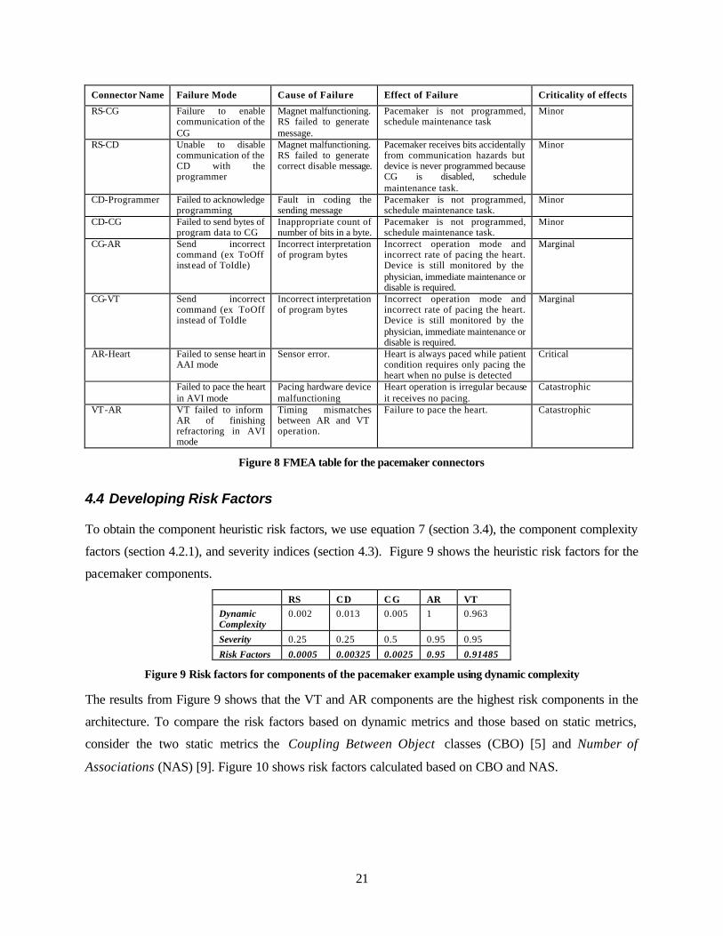
Figure 8 FMEA table for the pacemaker connectors

4.4 Developing Risk Factors

To obtain the component heuristic risk factors, we use equation 7 (section 3.4), the component complexity

factors (section 4.2.1), and severity indices (section 4.3). Figure 9 shows the heuristic risk factors for the

pacemaker components.

RS CD CG AR VT Dynamic Complexity

0.002 0.013 0.005 1 0.963

Severity 0.25 0.25 0.5 0.95 0.95

Risk Factors 0.0005 0.00325 0.0025 0.95 0.91485

Figure 9 Risk factors for components of the pacemaker example using dynamic complexity

The results from Figure 9 shows that the VT and AR components are the highest risk components in the

architecture. To compare the risk factors based on dynamic metrics and those based on static metrics,

consider the two static metrics the Coupling Between Object classes (CBO) [5] and Number of

Associations (NAS) [9]. Figure 10 shows risk factors calculated based on CBO and NAS.

22

RS CD CG AR VT CBO 0.47 0.8 1 0.6 0.6

NAS 0.75 0.75 1 0.75 0.75

Severity 0.25 0.25 0.5 0.95 0.95

Risk factors based on CBO

0.119 0.2 0.5 0.57 0.57

Risk factors based on NAS

0.1875 0.1875 0.5 0.71 0.71

Figure 10 Risk factors for components of the pacemaker example using static complexity

Figure 11 compares the risk factors based on static and dynamic metrics. It is obvious from the figure that

using dynamic metrics distinguishes the AR and VT components as high-risk components as compared to

RS, CD, and CG components. Using static metrics does not significantly distinguish the AR and VT as

high-risk components from the rest of the components, in fact, CG is considered at the same risk level as

the AR and VT if risk factors are based on static metrics. In the pacemaker architecture, AR and VT

components control the operation of the heart and hence they are the highest risk components. CG

controls the programming, which is monitored by the physician before the device is put into operation.

Though these results strengthen the rationale for using dynamic metrics as opposed to static metrics, they

are insufficient, as results from a single case study, to draw a general meaningful conclusion that dynamic

metrics are correlated to probability of failures. Application of the methodology to multiple case studies

would provide more evidence to support/weaken the decision of using dynamic metrics, this is the subject

of future empirical validation studies.

Figure 11 Comparison between risk factors using dynamic and static metrics

0

0.1

0.2

0.3

0.4

0.5

0.6

0.7

0.8

0.9

1

RS CD CG AR VT

Ris

k F

acto

rs

Dynamic

CBO

NAS

23

To obtain the connector heuristic risk factors, we use equation 7 (section 3.4), the connector complexity

factors (section 4.2.2), and severity indices (section 4.3). Figure 12 illustrates the heuristic risk factors for

the pacemaker connectors.

Connector Risk Factors RS CD CG AR VT Programmer Heart

RS 0.00035 0.00035

CD 0.00075 0.00275

CG 0.0005 0.0007 0.0007

AR 0.2375 0.95 VT 0.2565 0.82935 Programmer 0.00035 .0015

Heart 0.11685 0.29165

Figure 12 Risk factors for connectors in the pacemaker example

From Figure 12, we can identify connectors of highest risks that deserve more development resources and

testing. High risk connectors indicate that the interfaces and the communication protocol of messages

exchanged over that connector should be carefully implemented. Figure 12 illustrates that the connectors

between VT, AR, and the Heart are those of the highest risk in the architecture.

24

4.5 Constructing the pacemaker's CDG

Using the guidelines of section 3.5 and in [33], we develop the CDG for the pacemaker using the six

scenarios (Programming, AVI, VVI, VVT, AAI, and AAT). Figure 13 illustrates the CDG for the

pacemaker. We use the pacemaker's CDG to conduct risk analysis as described in the following section.

Figure 13 The CDG for the pacemaker example

4.6 Performing Risk Analysis

We implemented the algorithm defined in section 3.6, and applied it to the CDG of the pacemaker shown

in Figure 13. In this section, we discuss two types of analysis: risk assessment and sensitivity analysis.

These analysis methods make use of the algorithm and the pacemaker CDG described earlier.

4.6.1 Risk Assessment

We can use the algorithm as applied to the CDG graph to assess the overall risk of the pacemaker as an

aggregation of the risk factors of components and connectors in the architecture. This gives an overall

estimate of the risk of the pacemaker that is found to be ~ 0.9. This indicates that the pacemaker

architecture is very critical and failures are most likely to be catastrophic.

Using the algorithm and the graph to aggregate risk factors is useful for analyzing the risks in complex

hierarchical systems. Such systems are usually decomposed into subsystems where each subsystem is

composed of a number of components. We can apply the proposed methodology to various individual

subsystems (which have their own CDGs). We obtain a risk factor for a subsystem using risk factors of its

<Prog., 0,5>

<RS,5x10-4,5>

<CD, 3x10-3,5>

<AR,0.95,40> <VT,0.9,40>

<Heart,0,5> <CG, 2.5x10-2,5>

s

t

t

t <, 0, .01>

<, 0, .64>

<, 0, .35>

<, 0, .01> <, 0, .99>

<, 0, .99>

<, 0, .99>

<, 0, .99>

<, 0, .34> <, 0, .36>

<,3.5x10-4, .002>

<,1.5x10-3,.008>

<,2.7x10-3,.008>

<,7.5x10-4,.002>

<,3.5x10-4,.005>

<,3.5x10-3,.005> <,7x10-4,.0025>

<,5x10-4,.005>

<,7x10-4,.0025>

<,.12,.35> <,.29,.64>

<,.26,.29>

<,.95,.47>

<,.24,.19>

<,.26,.29>

25

individual components. Then we use the results to compare subsystems risk factors; i.e. relative ranking

of subsystem risk factors as opposed to calculating one factor for the system risk. The application of this

approach to large hierarchical system is the subject of future work.

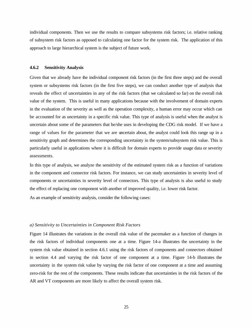
4.6.2 Sensitivity Analysis

Given that we already have the individual component risk factors (in the first three steps) and the overall

system or subsystems risk factors (in the first five steps), we can conduct another type of analysis that

reveals the effect of uncertainties in any of the risk factors (that we calculated so far) on the overall risk

value of the system. This is useful in many applications because with the involvement of domain experts

in the evaluation of the severity as well as the operation complexity, a human error may occur which can

be accounted for as uncertainty in a specific risk value. This type of analysis is useful when the analyst is

uncertain about some of the parameters that he/she uses in developing the CDG risk model. If we have a

range of values for the parameter that we are uncertain about, the analyst could look this range up in a

sensitivity graph and determines the corresponding uncertainty in the system/subsystem risk value. This is

particularly useful in applications where it is difficult for domain experts to provide usage data or severity

assessments.

In this type of analysis, we analyze the sensitivity of the estimated system risk as a function of variations

in the component and connector risk factors. For instance, we can study uncertainties in severity level of

components or uncertainties in severity level of connectors. This type of analysis is also useful to study

the effect of replacing one component with another of improved quality, i.e. lower risk factor.

As an example of sensitivity analysis, consider the following cases:

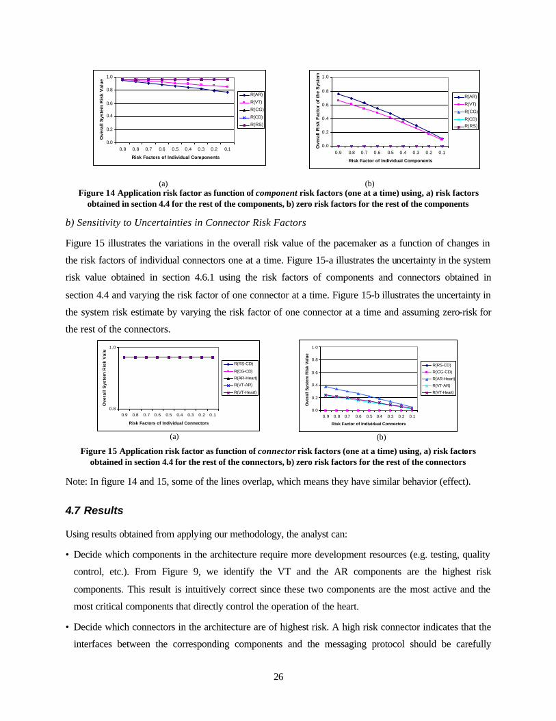
a) Sensitivity to Uncertainties in Component Risk Factors

Figure 14 illustrates the variations in the overall risk value of the pacemaker as a function of changes in

the risk factors of individual components one at a time. Figure 14-a illustrates the uncertainty in the

system risk value obtained in section 4.6.1 using the risk factors of components and connectors obtained

in section 4.4 and varying the risk factor of one component at a time. Figure 14-b illustrates the

uncertainty in the system risk value by varying the risk factor of one component at a time and assuming

zero-risk for the rest of the components. These results indicate that uncertainties in the risk factors of the

AR and VT components are more likely to affect the overall system risk.

26

Figure 14 Application risk factor as function of component risk factors (one at a time) using, a) risk factors obtained in section 4.4 for the rest of the components, b) zero risk factors for the rest of the components

b) Sensitivity to Uncertainties in Connector Risk Factors

Figure 15 illustrates the variations in the overall risk value of the pacemaker as a function of changes in

the risk factors of individual connectors one at a time. Figure 15-a illustrates the uncertainty in the system

risk value obtained in section 4.6.1 using the risk factors of components and connectors obtained in

section 4.4 and varying the risk factor of one connector at a time. Figure 15-b illustrates the uncertainty in

the system risk estimate by varying the risk factor of one connector at a time and assuming zero-risk for

the rest of the connectors.

Figure 15 Application risk factor as function of connector risk factors (one at a time) using, a) risk factors obtained in section 4.4 for the rest of the connectors, b) zero risk factors for the rest of the connectors

Note: In figure 14 and 15, some of the lines overlap, which means they have similar behavior (effect).

4.7 Results

Using results obtained from applying our methodology, the analyst can:

• Decide which components in the architecture require more development resources (e.g. testing, quality

control, etc.). From Figure 9, we identify the VT and the AR components are the highest risk

components. This result is intuitively correct since these two components are the most active and the

most critical components that directly control the operation of the heart.

• Decide which connectors in the architecture are of highest risk. A high risk connector indicates that the

interfaces between the corresponding components and the messaging protocol should be carefully

0.0

0.2

0.4

0.6

0.8

1.0

0.9 0.8 0.7 0.6 0.5 0.4 0.3 0.2 0.1

Risk Factors of Individual Components

Ove

rall

Sys

tem

Ris

k V

alu

eR(AR)

R(VT)

R(CG)

R(CD)

R(RS)

0.0

0.2

0.4

0.6

0.8

1.0

0.9 0.8 0.7 0.6 0.5 0.4 0.3 0.2 0.1

Risk Factor of Individual Components

Ove

rall

Ris

k F

acto

r o

f th

e S

yste

m

R(AR)

R(VT)

R(CG)

R(CD)R(RS)

0.8

1.0

0.9 0.8 0.7 0.6 0.5 0.4 0.3 0.2 0.1

Risk Factors of Individual Connectors

Ove

rall

Sys

tem

Ris

k V

alu

e

R(RS-CD)

R(CG-CD)

R(AR-Heart)

R(VT-AR)

R(VT-Heart)

0.0

0.2

0.4

0.6

0.8

1.0

0.9 0.8 0.7 0.6 0.5 0.4 0.3 0.2 0.1

Risk Factor of Individual Connectors

Ove

rall

Sys

tem

Ris

k V

alue

R(RS-CD)

R(CG-CD)

R(AR-Heart)

R(VT-AR)

R(VT-Heart)

(a) (b)

(a) (b)

27

designed. From Figure 12, we identify that the connection between the VT, AR, and Heart components

are the highest risk connectors. This result is intuitively correct in the context of the pacemaker example

since these connectors deliver critical messages controlling the heart operation such as sensing and

pacing.

• Study how uncertainties in component risk factors affect the overall risk value of the system. From

Figure 14, we identify that the increase in the risk factors VT and the AR components highly affect the

risk factor of the system as compared to any increase in the risk factors of the CD, CG, or RS

components which have almost negligible effect.

• Study how uncertainties in connector risk factors affect the overall risk value of the system. From

Figure 15-a, we identify that uncertainties in the connectors risk factors do not have a significant impact

on the estimated risk factor of the system. However, if we consider zero-risk for the rest of the

component and connectors, we find that the increase in the risk factor of connection between AR and

Heart components highly affect the risk factor of the system as compared to any increase in the risk

factors of the connection between CG and CD. This could be interpreted for the pacemaker example as

follows: in the context where risk factors of components are considered, the system risk becomes more

dependent on the component risk factors rather than the connector risk factors.

5 Related Work

In this paper, we present a methodology for risk assessment that uses dynamic complexity metrics and

severity ranking. In the sequel we summarize research work related to this work.

Complexity metrics provide substantial information for distinguishing differences between software

systems whose reliability is being modeled. There are some predictive models that incorporate a

functional relationship between program errors measures and software complexity metrics [14]. Software

complexity measures are also used for developing and executing test suites [10]. Therefore, static

complexity is used to assess the quality of a software. The level of exposure of a module is a function of

its execution environment. Hence, dynamic complexity [13] evolved as a measure of complexity of the

subset of code that is actually executed. Dynamic complexity was discussed by Munson et.al. [18] for

reliability assessment purposes. The authors emphasize that it is essential to not only consider complex

modules but how frequently they are executed. They define execution profiles for modules that reflect

what percentage of time a module is executing, and hence derived functional complexity and operational

complexity as dynamic complexity metrics. Ammar et.al. [2] extend dynamic complexity definitions to

incorporate concurrency complexity. They further use Coloured Petri Nets models to measure dynamic

complexity of software systems using simulation reports. Yacoub et. al. [34] define dynamic metrics that

28

include dynamic complexity and dynamic coupling metrics to measure the quality of architectures. Their

approach is based on dynamic execution of UML statechart specification of a component and the

complexity metrics proposed is based on simulation reports. In this paper, we use dynamic metrics as

measures of the components and connectors complexities.

The work by Kazman et.al. [39] addresses the problem of measuring architecture complexity. The

approach involves determining the proportion of the architecture covered by particular patterns

(architecture regularity), and the number of different types of patterns composing the architecture. A

pattern recognition system is used to analyze the regularity of the architecture and to explore some

properties such as fan-in and fan-out of elements (i.e., the number of elements that control, or are

controlled by, an element, respectively), and particular design problems (e.g., layer bridging). The

Architecture Trade-Offs Analysis Method (ATAM) [40] is concerned with the development of techniques

and models to assess and evaluate software architectures with respect to analytical attributes such as

performance and availability and other qualitative attributes based on formal inspections such as

modifiability, safety, and security. The methodology is heavily scenario-based, it uses attribute-specific

questions to ensure proper coverage of an attribute by a specific scenario. Each component is then

assigned a quality measure that is a combination of the quality attributes gathered from answers to the

attribute-specific questions. The ATAM method helps in discovering risks at early development stages,

and in defining sensitivity and trade-off points (points where change could affect multiple attribute) in a

candidate architecture. Although the technique formalizes the steps of evaluating an architecture, it is still

mostly qualitative (a question-answer approach).

Criticality analysis has gained the interest of many researches and has been integrated in FMEA

procedures, i.e. Failure Mode Criticality and Effect Analysis (FMECA). In FEMCA, severity of the effect

of failures is considered. The most commonly used methods for assessing criticality in FEMCA are : Risk

Priority Number (RPN) [25], the MIL_STD 1629A Criticality Number ranking [7], and the multi-criteria

Pareto ranking [26]. In RPN, the risk number is function of occurrence ranking, severity ranking, and

detection ranking. In the MIL_STD 1629A FMECA, criticality number is function of failure mode ratio,

failure effect probability, failure rate of the component, and time period of interest. Pareto ranking is an

enhancement to the MIL_STD 1629A FMECA criteria in which severity is measured on a ratio scale

instead of ordinal scale. These methods are mostly developed for hardware design and manufacturing.

The main drawback of these method is that they use failure rate values or probability of failure which are

difficult to estimate. In our study, we use factors that affect the probability of finding fault and executing

that fault, i.e., dynamic metrics.

There are several ongoing fault-risk assessment approaches and tools that mainly uses static product

metrics or process metrics. For example, the Nortel's Enhanced Measurement for Early Risk Assessment

29

of Latent Defects system, EMERALD, is an example of an analysis system in production use for

assessing the risk of faults [11]. Bellcore's Analyzer for Reducing Module Operational Risk, ARMOR, is

a prototype software-risk analysis tool [16]. Bellcore's Software Architecture Based Analysis, SABA,

technology has been integrated into Lucent Technologies' software update risk assessment process [22].

The CDGs used in our methodology resembles the task and function graphs developed by Smith et. al.

[38] for performance engineering, where function times are estimated and then the overall time of the

application is estimated from the graphs. The proposed risk analysis methodology and the performance

engineering methodology both use estimates for component (module) execution times. However, the

proposed methodology is concerned with reliability risk analysis while Smith’s methodology is more

concerned with performances analysis of architectures.

6 Conclusion and Future Work

This paper presents a methodology for risk analysis of software architectures. The proposed methodology

is based on the statechart specification of individual components and on the scenarios of component

interactions. The execution profiles of these scenarios are assumed to be available. We develop a risk

analysis model and a risk aggregation algorithm that we use to perform risk assessment and risk analysis.

A simple case study is used to illustrate the applicability of the approach.

The proposed methodology has the following benefits:

• The methodology is applicable early at the architectural level and hence it is possible to identify critical

components and connectors early in the lifecycle. Those components would require further

development resources in terms of design, implementation, testing, etc.

• The methodology is based on dynamic metrics. We use dynamic metrics to account for the fact that a

fault in a frequently executed component will frequently manifest itself into a failure. Results from the

pacemaker example (shown in Figure 11) illustrate the benefits of using dynamic metrics.

• The methodology is based on simulation of architecture models. Simulation helps in:

1. Performing FMEA procedures because it minimizes the effort required to analyze the effect of

failures. The analyst can inject faults and study their effect by simply running the simulator and

observing simulation outputs and reports.

2. Calculating the CDG parameters such as probability of transitions that is based on number of

messages transmitted from one component to another.

• The methodology is automatable. We have implemented the algorithm and used it in our case study.

Also, we obtain measurement values for dynamic metrics using simulation reports.

30

We identified the following issues that could be addressed as future work:

• We use an ordinal scale for measuring severity and assign severity indices to each category. To develop

risk factors we combine complexity factor (ratio scale) with severity factor (ordinal scale). This

problem is common to many risk assessment methods [25, 7]. The Pareto ranking [26] uses ratio scale

with severity, but it is confronted with the problem of defining boundaries between various severity

categories. Perhaps one solution is to apply the same methodology discussed above to each risk

category separately. In this case, severity ratios can be developed under each of the severity categories,

catastrophic, critical, marginal, and minor, such that components and connectors are compared within

one category and not across categories (i.e. a ratio scale under each ordinal category).

• We developed the CDGs for the pacemaker example manually from simulation reports and scenarios.

Automating the development of CDGs would promote the application of our methodology. Towards the

automation of the methodology, we developed a utility that processes simulation logs and automatically

produces measurement values for the dynamic metrics for components and connectors. We also

developed a utility that allows the domain expert to feed in data such as the operational profile for

system usage and severity indices and automatically get parameters for the CDG such as risk factors for

components and connectors. In the future, we plan to automate the construction of the graph nodes and

links and provide a GUI that presents to the analyst the CDGs for the system and its subsystems and the

associated graphical representations of the risk analysis results.

• Another area that is worth investigation is studying the effect of uncertainties in some parameters such

as the scenario probabilities and the estimated average execution times. Future work would investigate

the effect of these parameters on the system risk estimate.

• We applied the methodology to the pacemaker case study. Future research could experiment with

applying the methodology to larger case studies with multiple subsystem to compare the aggregated risk

factors of individual subsystem.

References

[1] R. Allen and D. Garlan. A Formal Basis for Architectural Connection. ACM Transaction on Software Engineering and Methodology, 6(3):213-249, July 1997. [2] H. Ammar, T. Nikzadeh, and J. Dugan. A Methodology for Risk Assessment of Functional Specification of Software Systems Using Coherent Petri Nets. Proceedings of the Fourth International Software Metrics Symposium, Metrics'97, Albuquerque, New Mexico, Nov 5-7, 1997, pp108-117. [3] L. Bass, P. Clements, and R. Kazman. Software Architecture in Practice. Addison Wesley Longman, 1998. [4] J. Bowles. The New SEA FMECA Standard. Proceedings of the 1998 Annual Reliability and Maintainability Symposium, Anaheim, California, January 1998 pp 48-53.

31

[5] S. Chidamber and C. Kemerer. A Metrics Suite for Object Oriented Design. IEEE Transactions on Software Engineering, Vol 20, No 6, June 1994, pp476-493. [6] B. Douglass. Real-Time UML : Developing Efficient Objects for Embedded Systems. Addison-Wesley, 1998. [7] Procedures for Performing Failure Mode Effects and Criticality Analysis. US MIL_STD_1629 Nov 1974, US MIL_STD_1629A Nov 1980, US MIL_STD_1629A/Notice 2 Nov 1984. [8] D. Harel. Statecharts: A Visual Formalism for Complex Systems. Science of Computer Programming, July 1987, pp231-274. [9] R. Harrison S. Counsell, and R. Nithi. Coupling Metrics for Object Oriented Design. Proceedings of the 5th Metrics Symposium, Bethesda, Maryland, Nov 20-21, 1998, pp150-157. [10] D. Heimann. Using Complexity Tracking in Software Development. Proceedings of the 1995 Annual Reliability and Maintainability Symposium, 1995, pp433-437. [11] J. Hudepohl, S. Aud, T. Khoshgoftaar, E. Allen, and J. Mayrand. Emerald: Software Metrics and Models on the Desktop. IEEE Software, 13(5):56-60, Sept. 1996. [12] International Telecommunication Union (ITU-T) Recommendation Z.120 (10/96) for Message Sequence Charts (MSC). http://www.itu.int/itudoc/itu-t/rec/z/z120.html [13] T. Khoshgoftaar, J. Munson, and D. Lanning. Dynamic System Complexity. Proceedings of the International Software Metrics Symposium, Metrics'93, Baltimore MD., May 1993, pp129-140. [14] T. Khoshgoftaar and J. Munson. Predicting Software Development Errors using Software Complexity Metrics. In Proceedings of the 1995 Software Reliability and Testing, IEEE Computer Society Press, 1995, pp20-28. [15] H. Kumamoto and E. Henley. Probabilistic Risk Assessment for Engineers and Scientists, second edition IEEE Press, 1996. [16] M. Lyu, J. Yu, E. Keramidas, and S. Dalal. Armor: Analyzer for Reducing Module Operational Risk. In Proceedings of the Twenty-Fifth International Symposium on Fault-Tolerant Computing, pages 137-142, Pasadena, CA, June 1995. [17] N. Medvidovic and R. N. Taylor. A Classification and Comparison Framework for Software Architecture Description Languages. IEEE Transactions on Software Engineering Vol 26, No. 1, January 2000, pp70-93. [18] J. Munson and T. Khoshgoftaar. Software Metrics for Reliability Assessment. In Handbook of Software Reliability Engineering, Michael Lyu (edt.), McGraw-Hill, 1996, Chapter 12, pp 493-529 [19] J. Musa, G. Fuoco, N. Irving, D. Kropfl, and B. Julin. The Operational Profile. In the Handbook of Software Reliability Engineering, Michael R. Lye (edt.), McGraw-Hill, New York, NY, 1996, Ch.5, pp167-216. [20] Software Safety, Nasa Technical Standard. NASA-STD-8719.13A, September 15, 1997 http://satc.gsfc.nasa.gov/assure/nss8719_13.html [21] ObjecTime User Guide. ObjecTime Ltd., Kanata, Ontario, Canada, 1998. [22] K. Rauscher and D. Rak. Gray box Risk Assessment for Telecommunications Software Modifications. In IEEE International Conference on Communications Conference Record, Volume 1, pages 208-213, Dallas, TX, June 1996. [23] NASA's Definition of Risk Matrix, http://tkurtz.grc.nasa.gov/risk/rskdef.htm [24] Rational Rose Real-Time. http://www.rational.com/products/rosert/index.jtmpl [25] Potential Failure Mode and Effect Analysis in Design (Design FEMCA) and Potential Failure Mode and Effects Analysis in Manufacturing and Assembly Process (Process FEMCA) Reference Manual. Society of Automotive Engineering, Surface Vehicle Recommended Practice, J1739, July 1994.

32

[26] Recommended best practices for Failure Mode, Effects, and Criticality Analysis Procedures. Socie ty of Automotive Engineering, Aerospace recommended practice, forthcoming 1999. [27] B. Selic, G. Gullekson, and P. Ward. Real-Time Object Oriented Modeling. John Wiley & Sons, Inc. 1994. [28] M. Shaw and D. Garlan. Software Architecture: Perspectives on an Emerging Discipline. Prentice Hall Upper Sadle River, NJ 1996. [29] The Unified Modeling Language Resource Center http://www.rational.com/uml/ index.html [30] S. Vestal. A Cursory Overview and Comparison of Four Architecture Description Languages. Honeywell Technology Center, Technical Report February 1993. [31] K. Weidenhaupt, K. Pohl, M. Jarke, and P. Haumer. Scenarios in System Development: Current Practice. IEEE Software, March/April 1998, pp34-45. [32] S. Yacoub and H. Ammar. A Matrix-Based Approach to Measure Coupling in Object-Oriented Designs. Journal of Object Oriented Programming, JOOP, October, 2000. [33] S. Yacoub, B. Cukic, and H. Ammar. Scenario-based Reliability Analysis of Component-Based Software. Proceedings of the Tenth International Symposium on Software Reliability Engineering, ISSRE'99, Boca Raton, Florida USA, November 1-4 1999, pp22-31. [34] S. Yacoub, H. Ammar, and T. Robinson. Dynamic Metrics for Object Oriented Designs. Proceedings of the Sixth International Symposium on Software Metrics, Metrics'99, Boca Raton, Florida USA, November 4-6 1999, pp50-61. [35] S. Yacoub, B. Cukic, and H. Ammar. A Component-Based Approach to Reliability Analysis of Distributed Software Systems. Proceedings of the 18th IEEE Symposium On Reliable Distributed Systems, SRDS'99, Lausanne Switzerland, October 19-22, 1999, pp158-167. [36] H. Ammar, B. Cukic, C.Fuhrman, and A. Mili. A Comparative Analysis of Hardware and Software Fault Tolerance: Impact on Software Reliability Engineering. Annals of Software Engineering. Volume 10, Spring 2000. [37] H. H. Ammar, T. Nikzadeh, and J. B. Dugan. Risk Assessment of Software Systems Specifications. IEEE Transactions on Reliability, Vol. 49, To appear, Fall 2000. Preliminary parts of this paper have been published in Proceedings of the International Symposium On Software Reliability Engineering (ISSRE'97), and the Fourth International Software Metrics Symposium (Metrics'97). [38] L.G. Williams and C.U. Smith. Performance Engineering of Software Architectures. Proceedings of the Workshop on Software and Performance, Santa Fe, NM, Oct. 1998. [39] R. Kazman and M. Bruth. Assessing Architectural Complexity. In Proceedings of the 2nd European Conference on Software Maintenance and Engineering, pp 104-112, Florence, Italy, March 1998. [40] R. Kazman, M. Klein, M. Barbacci,H. Lipson, T. Longstaff, and S. Carriere. The Architecture Tradeoff Analysis Method. Proceedings of the 4th International Conference on Engineering of Complex Computer Systems, ICECCS’98, Monterey CA, August 1998.

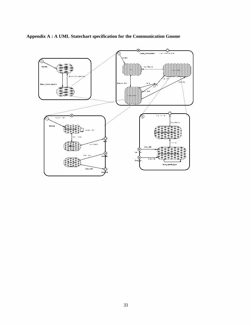
33

Appendix A : A UML Statechart specification for the Communication Gnome

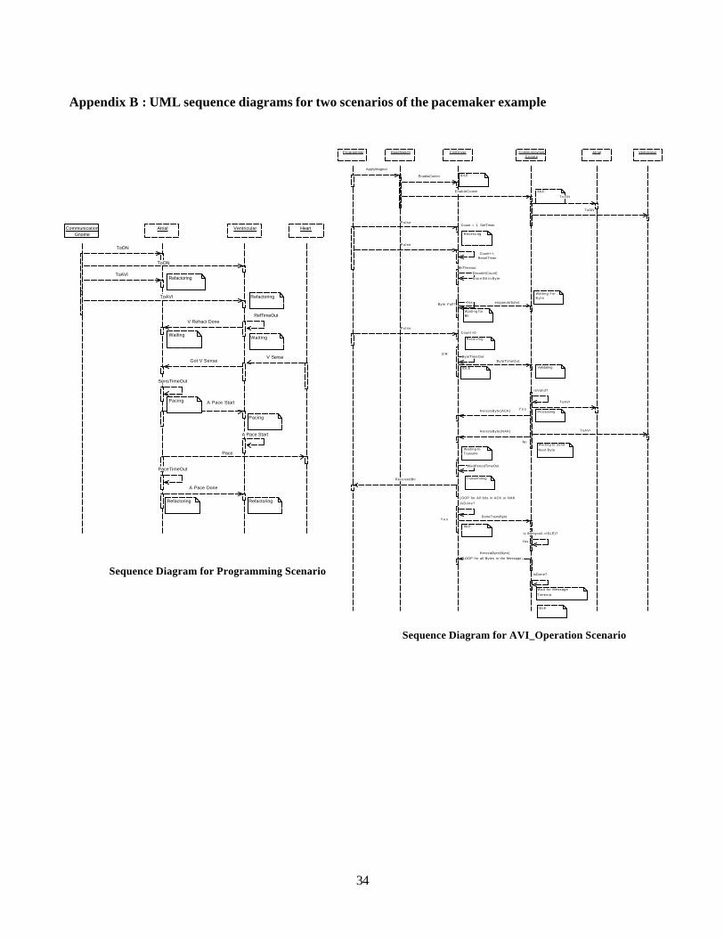
34

CommunicationGnome

Atrial Ventricular Heart

ToON

ToON

ToAVI

ToAVI

Refactoring

Refactoring

V SenseGot V Sense

RefTimeOut

Waiting

V Refract Done

Waiting

SensTimeOut

A Pace Start

A Pace Start

Pacing

Pacing

PaceTimeOut

A Pace Done

Refactoring Refactoring

Pace

Sequence Diagram for AVI_Operation Scenario

Sequence Diagram for Programming Scenario

Programmer ReedSwitch CoilDriver CommunicationG n o m e

Atrial Ventricular

ApplyMagnet

EnableComm

EnableComm

Pu lse

Receiv ing

IDLE

Pu l se

Count++,ResetTimer

BitTimeout

Decode(Count)

Store Bit in Byte

Byte Full? enqueue(byte)Yes

ByteTimeOut

Waiting for Bit

IDLE

Count = 1, SetTimer

Pu l seCount =0

Receiving

ByteTimeOut

O R

IDLE

Waiting For B y t e

Validating

IsValid?

Processing

ToAVI

ToON

ToON

ToAVI

Y e sHerezaByte(ACK)

No

HerezaByte(NAK)

Waiting to Transmit

Waiting to Send

Next Byte

WaitPeriodTimeOut

TransmittingReceivedBit

IsDone?

DoneTransByteY e s

is IN(mycoil->IDLE)?

Yes

HerezaByte(Byte)

LOOP for All bits in ACK or NAK

LOOP for all Bytes in the Message

IsDone?

Wait for Message

Timeout

IDLE

IDLE

Appendix B : UML sequence diagrams for two scenarios of the pacemaker example

35

Acronyms

ADL Architecture Description Language AR Atrial_Model, a component in the pacemaker architecture CBO Coupling Between Object classes, an OO design metric CD Coil_Driver, a component in the pacemaker architecture CDG Component Dependency Graph CG Communication_Gnome, a component in the pacemaker architecture FEMA Failure Mode and Effect Analysis FMECA Failure Mode Criticality and Effect Analysis MSC Message Sequence Charts NAS Number of Associations, an OO design metric ROOM Real-time Object Oriented Modeling RPN Risk Priority Number RS Reed_Switch, a component in the pacemaker architecture UML Unified Modeling Language VT Ventricular_Model, a component in the pacemaker architecture Notations

S A set of scenarios Sk Scenario number k |S| Total number of scenarios PSk Probability of scenario number k AEappl Average execution time of a scenario s A start node in a CDG t A termination node in a CDG N A set of nodes in a CDG, N={n} n A node in a CDG. E A set of edges in a CDG, E={e}. RCI A parameter in the CDG, the reliability estimate of component Ci ECi A parameter in the CDG, the average execution time of the component Ci Tij A parameter in the CDG, the name of the transition from node ni to nj, RTij A parameter in the CDG, the reliability estimate of a transition from node ni to node nj. PTij A parameter in the CDG, the probability of a transition from node ni to node nj. Ci Component number i svrty I Severity factor for component Ci hrf I Heuristic risk factor for component Ci hrf ij Heuristic risk factor for the connector between the components Ci and Cj. cpxk(Ci) Complexity of component Ci in scenario Sk. cpx(Ci) Complexity of component Ci ECk(Ci,Cj) Export coupling for component Ci with respect to component Cj in scenario Sk EC(Ci,Cj) Export coupling for component Ci with respect to component Cj Mk(Ci,Cj) The set of messages sent from component Ci to component Cj during the execution of

scenario Sk MTk The total number of messages exchanged between all components during the execution of

scenario Sk VG Cyclomatic complexity of a graph.

Appendix C : Acronyms and Notation

36

Sherif Yacoub is a member of the Technical Staff at Hewlett-Packard Laboratories, Palo Alto,

California. Dr. Yacoub earned a Ph.D. in computer engineering from the department of Computer Science

and Electrical Engineering at West Virginia University in 1999, where he worked as a Research Assistant

Professor until July 2000. He received an MSc. in electrical engineering in 1997 and a BSc in computer

engineering in 1994 from Cairo University, Egypt, where he also lectured in software engineering. Dr.

Yacoub is a member of the IEEE and the ACM professional organizations. His research interests include

software design, design patterns, software reuse at the architectural level, document understanding, design

quality, risk analysis, and software reliability. Contact him at sherif_yacoub@hp.com

Hany Ammar is an Associate Professor of Computer Engineering in the department of Computer

Science and Electrical Engineering at West Virginia University. He joined the faculty at WVU in 1990

after five years of service on the faculty at Clarkson University. Dr. Ammar has published over 76 articles

in prestigious journals and conference proceedings such as the IEEE Transaction on Software

Engineering and the IEEE Transactions on Reliability. Dr. Ammar is a member of the IEEE and the ACM

professional organizations. He has served as the Chairman of the Upper Monongahela Subsection of the

Pittsburgh section of the IEEE, as a Director of the Pittsburgh section of the IEEE , and the student

section advisor of the IEEE Computer Society at WVU.

37

Contact Information

Name: Sherif M. Yacoub

Mailing Address: Hewlett-Packard Labs

1501 Page Mill Rd.

MS 1L-15

Palo Alto, CA 94304, USA

E-Mail: sherif_yacoub@hp.com

Phone: 650 857 2765

Fax: 650 852 2986

Name: Hany H. Ammar

Mailing Address: Department of Computer Science and Electrical Engineering

West Virginia University

Morgantown, WV 26506-6109

E-Mail: hammar@wvu.com

Phone: 304 293 - 0405 ext. 2514

Fax: 304 293-8602