a method of structural load prediction for high-speed ... craft loads.pdf · a method of structural...

A Method of Structural Load Prediction for High-Speed Planing Craft Richard H. Akers, P.E. (SNAME M)

Maine Marine Composites LLC, Portland, Maine, USA

The lack of information about hydrodynamic loads is an obstacle in the structural design of high-speed planing boats. A method

is proposed to derive panel pressures from a time-domain motion simulator. The simulator predicts planing boat motion by

calculating forces using first principles and semi-empirical algorithms, combining the forces, and integrating the results to solve

the equations of motion. Integral to the time-domain simulator algorithm is a calculation of longitudinal pressures at every

timestep. The sectional pressures are expanded into transverse pressure distributions using models from Smiley (1951) for

transverse pressure distributions in the forward, chines-dry region and the aft, chines-wet region. A load-mapping software tool

transfers pressure distributions to a finite element analysis program. Three validation efforts were performed by comparing

simulated and measured quasi-static hull pressures published for a prismatic planing hull and a 20.5 foot fiberglass ski boat

operating at constant speeds, and dynamic pressures on the hull of a recreational aluminum fishing boat operating in waves.

INTRODUCTION The objective of this project is to develop and verify a practical

method to use time domain simulation to drive structural design

of high speed planing craft. Existing and developmental time-

domain simulators will be enhanced and modified so as to

calculate panel pressures, vessel kinematics, and loads for use in

Finite Element Method (FEM) programs for structural analysis.

Specifically, low aspect ratio strip theory will be extended to

predict transient slamming loads created when a high-speed

craft travels through irregular seas. The new analysis method

must meet the following requirements:

Predict transient hydrodynamic panel pressures for use in

Finite Element Method programs.

Predict velocities, rates and accelerations for use in FEM

programs.

Calculate instantaneous shear forces and longitudinal

bending moments for comparison and verification of results.

Maine Marine Composites (MMC) has been working

continuously for almost two decades on a computer program to

predict the surge, heave and pitch motion of a planing boat in

regular and irregular seas. The simulator was developed from

algorithms described in a computer program developed and

published by Ernest Zarnick (1978) of David W. Taylor Naval

Ship R & D Center. Instantaneous motions of a planing boat are

predicted by:

Calculating the forces on each one of hundreds of

hydrodynamic stations (sections) by using the following

algorithms: impacting wedge, linear 2D buttock flow,

viscous drag using Reynold’s Number-based drag

coefficients, and crossflow drag in fully-wetted regions

Adding the sectional force components together in a

weighted sum using weighting coefficients derived from

more than 100 model and full-scale tests

Calculating the added mass for each section using empirical

formulas based on the sectional deadrise

Integrating the forces and added masses for each degree of

freedom

Multiplying the inverted mass matrix times the force vector

to obtain the accelerations in surge, heave and pitch; and

then integrating the accelerations to find velocities and rates,

and then integrating again to find positions and angles.

In the Ship Structures Committee (SSC) Project SR-1470 the

time-domain simulator program was modeled to export point

pressures within an operator-specified subset of the entire

geometric mesh describing the hull. With some interpolation to

match the pressures obtained from the simulator with the mesh

used in the FEM analysis, the strain in the structural panels of

the planing boat can be predicted. This strain can be used to test

the capability of the boat hull to withstand a particular sea state

without damage.

The specific goal of this SSC project was to show that sectional

pressures calculated by the simulator can be converted to panel

pressures which can be used in a Finite Analysis Method (FEM)

program to predict stress and strain in the hull structure.

Background There is on-going interest in high-speed planing boats,

especially for government patrol boats. The USCG is in the

middle of a long-term acquisition program for the RB-S and

RB-M patrol craft. USSOCOM has issued a contract for the

CCM Mark I, a replacement craft for the workhorse 11m RIB.

In the civilian sector, high-speed craft are important for new,

competitive ferry services and possibly for high-speed freight

services, both regulated by US Coast Guard.

Structural assessment of these craft has an important impact on

their operational safety. A major problem in the design of high-

speed planing boats such as fast ferries and patrol craft is

predicting the panel loads for structural analysis. It is very

difficult to predict the loads for quasi-static operation of planing

boats, and even more difficult to predict the instantaneous loads

in irregular sea states. Often techniques such as computational

fluid dynamics (CFD) are used to predict hydrodynamic loads,

but these methods are computationally intensive and cannot be

used in long time-domain simulations of planing craft.

To illustrate the difficulty of designing high-speed planing craft,

the Mk V is an 82-foot boat used by the Special Operations

Forces with an estimated top speed of 47-50+ knots in SS2, and

a cruising speed of 25-35 knots in SS3. A requirement for the

Mk V was that it be designed to meet the 1990 ABS Guide for

Building and Classing High Speed Craft (Codega, 2014). The

vessel's severe missions resulted in structural failures and

injuries to crew and passengers. Since that time ABS Guide has

evolved into the present-day version, Rules for Building and

Classing High Speed Naval Craft (ABS, 2014). Part 3, Chapter

2, Section 2, “Design Pressures,” of this standard addresses

2014 Ship Structure Symposium

SSC 2014 Akers of 24

bottom loading to be used for structural design. The primary

method of estimating pressures is to use formulas for bottom

slamming and hydrostatic pressure. These formulas have been

derived from a combination of first principle and empirical

methods, and are hull-location specific. Alternatively, the ABS

Rules (3-1-3, Section 9.1) state that hydrodynamic “… analysis

software formulations derived from linear idealizations [panel

methods and strip theory] are sufficient. Enhanced bases of

analysis may be required so that non-linear loads, such as hull

slamming, may be required. The adequacy of the selected

software is to be demonstrated to the satisfaction of ABS.”

These methods are efficient and appropriate for the design of

conventional boats to be used in well understood missions, but

may fall short for the design of new hullforms or structures

designed for new, demanding missions. A more accurate

method of predicting instantaneous, local structural loads is

required for the design of future high-speed patrol boats and

high-speed ferries.

Empirical algorithms have a limited range of applicability and

are not well suited to time domain simulation. Spencer (1975)

proposed a methodology for structural design of aluminum

crewboats using Savitsky's method (1964) to predict the trim

angle of the vessel, data from Fridsma (1971) to predict peak

accelerations, and a technique from Heller and Jasper (1960) to

predict hull pressure distributions. Given a pressure distribution,

engineers can calculate maximum frame spacings and minimum

panel thicknesses. This method is an historical basis for the

dynamic pressure used in the USCG's NVIC 11-80 (1980).

Unfortunately the method makes assumptions about sea states,

missions, and hull geometry. Any significant deviations from

these assumptions introduce uncertainty into the design process.

In 2005 SSC funded a project to study and compare "…the

application, requirements and methods for the structural design

of high speed craft..." used by various classification societies

(Stone, 2005). Classification society rules use empirical

formulas to predict vertical accelerations, which are used in

structural design calculations. A more direct method would be

to use time-domain simulation to predict panel pressures for

structural design.

According to Akers (1999a, 1999b) and Rosén (2004) planing

hull simulation programs based on low aspect ratio strip theory

have been in existence for several decades. These programs can

predict the vertical accelerations of a planing monohull

operating in a seaway with good engineering accuracy.

Justification for Project The ABS Rules for Building and Classing High Speed Naval

Craft (ABS, 2014) recognizes that time domain simulation is an

effective way of predicting hull pressures for structural analysis

of high speed craft. Section 3-1-3 of the Guide says:

“3.5.7(a) Global Slamming Effects. The simplified

formulae … may be used to account for global

slamming effects in the preliminary design stage. For

detailed analysis, a direct time-domain simulation

involving short-term predictions are to be used for the

global strength assessment of monohulls. In most cases

involving high speeds, the absolute motions or relative

motions will be of such large amplitude that nonlinear

calculations will be required...

“3.5.7(b) Local Impact Loads. Panel structures with

horizontal flat or nearly flat surfaces such as a wet

deck of a multi-hull craft will need to be

hydroelastically modeled, where in the dynamics of

the fluid and the elastic response of the plate and

stiffeners are simultaneously modeled."

SIMULATION OF PLANING HULLS The time-domain simulator used as the basis for this project

calculates sectional forces, integrates the forces longitudinally,

and solves for the boat accelerations. The primary goal of this

project is to expand the sectional forces into panel pressures

which can be used in structural analyses. At each time step the

time-domain simulator calculates sectional pressure

contributions from the following sources:

Impacting wedge (low aspect ratio strip theory).

Low aspect ratios 2D ideal flow to model buttock flow

Crossflow drag for sections in the chines-wet region

Viscous drag based on the mean wetted length

Hydrostatic buoyancy

The results are weighted and added together on a section-by-

section basis to calculate an array sectional force vectors.

At each time step, the simulator:

1. Calculates the force vector and moment vector

contributed by each station (refer to Appendix 1).

2. Calculates the added mass contributed by each station

3. Integrates the station force and moment vectors to find

the total force vector and moment vector

4. Integrates the added mass over the entire hull to find the

total added mass and added pitch inertia

5. Solves the equations of motion to find instantaneous

angular and radial accelerations:

|A| = (|M| + |Added M|)-1

* |Total Force/Moment|

6. Integrates the accelerations to find velocities and the

velocities/angular rates to find positions/angles

The sectional force and moment vectors calculated in Step 1 are

the basis for calculating the vector forces exported to FEA.

CALCULATING PRESSURES FOR

STRUCTURAL ANALYSIS

Figure 1 Planing Regions

The transverse pressure distributions can be categorized by their

region of operation (refer to Figure 1). Starting at the bow of the

Deck

Chine

Keel Calm

Waterline Chines-Dry

Region

Chines-Wet

Region



planing boat, the most forward wetted point on the keel occurs

at the calm waterline. Moving aftward, the water rises above the

calm waterline because the water displaced by the boat piles up

to port/starboard, resulting in an increase of the sectional draft.

Eventually the piled-up water reaches the chine. The “chines-

dry region” is the range between the most forward wetted point

and the station for which the pile-up water reaches the chine.

The transverse flow separates off of the chine, so the piled-up

water stops at the chine. The distance abaft the end of the

“chines-dry region” is, of course, called “chines-wet.”

From many model tests (e.g. Kapryan, 1955; Broglia, et. al.

2010) it is apparent that the transverse pressure distribution

follows a curve that resembles the curves in Figure 2. The

similarity between the pressure distributions at different

longitudinal locations is apparent in this figure. The

distributions with a peak occur in the “chines-dry” region, while

the ones without a peak occur in the “chines-wet” region.

Transverse Pressure Distribution As seen in Figure 2 the transverse pressure distribution in the

chines-dry region is dramatically different than that in the

chines-wet region. In the chines-dry region the pressure reaches

a peak value along a stagnation line and drops off quickly

toward the keel. After the stagnation line reaches the chine in

the chines-wet region, the pressure distribution becomes much

more constant, tapering off as it nears the chine.

Figure 2 Transverse pressure distribution measured on boat

with 0-heel angle. “y/B=0.05” is bow and “y/B=1.50” is stern

(Broglia, et. al., 2010, Figure 7). Curves with peaks are in

chines-dry region, curves at x/B=1.2 and 1.5 are in chines-wet

region.

The procedure for calculating pressure loads at any point on the

hull is to calculate the total sectional pressure (force/unit length)

and use the models summarized in Smiley (1951) to calculate a

transverse pressure distribution from the sectional forces.

Smiley suggests two different methods of modeling the pressure

distribution, one for the forward chines-dry region and one for

the aft chines-wet region of the boat.

Modeling the Transverse Pressure Distribution: Chines-Dry

Region

The transverse pressure distribution in the chines-dry region is

modeled using Equations 1, 2 and 3. The variable K is the

water-rise ratio.

(1)

The deadrise is assumed to be constant for each station,

defined as the angle between the keel point and the chine point.

For computational efficiency a spline curve is precalculated to

compute K from (refer to Figure 4).

Pierson (1948) and Pierson and Leshnover (1950) suggest

Equation 2 to calculate a modified deadrise θ taking into

account the running trim of the boat. The value K was

precalculated using the spline curve described above.

(2)

Smiley’s transverse pressure distribution uses this in the form of

cot() = 1/tan(). The transverse pressure distribution is

modeled by Equation 3 with an appropriate scale factor.

(3)

Equation 3 includes a variable which is related to the

transverse distance from the keel toward the chine. The term

(/c) represents the normalized wetted half beam ranging from 0

to 1. The equation goes to - when =c, corresponding to the

pressure at the outer edge of the wetted surface c. The pressure

curve passes through 0 close to that point, and the zero crossing

is the effective outer edge of the wetted beam model. In other

words the model is not accurate over the entire range of

normalized half beam, but has to be scaled slightly. A value is

defined that maps from the keel to the zero crossing.

At each time-step, the trim angle is known, so a second

constant c1 is calculated.

(4)

Instead of ranging from 0 to 1, the value of ranges from 0 to

as calculated as in Equation 5.

(5)

A factor of proportionality is chosen so that the integral of

Equation 3 from 0 to is equal to 1. The direct integral

of this formula can be shown to be Equation 6. The total

transverse pressure calculated by this formula over the entire

wetted beam is equal to the sectional pressure.

(6)

The scale factor required to make Equation 3 an equality

is . Figure 3 is a chart of the transverse pressure for

three different values of deadrise , all shown for a constant

trim = 4 degrees.



Figure 3 Sample chines-dry transverse pressure distributions for

three different deadrise angles. All three distributions were

calculated at a running trim of 4 degrees.

Modeling the Transverse Pressure Distribution: Chines-Wet

Region

The transverse pressure distribution in the Chines-Wet Region

does not have the bump at the stagnation line that the Chines-

Dry distribution has. Instead it starts with a flat region near the

keel and rolls off as it approaches the chine (refer to Figure 2,

curve “y/B=1.5”). Smiley (1951) uses the results of a derivation

from Korvin-Kroukovsky and Chabrow (1948) to model the

pressure distribution in the chines-wet region. Variables in the

following equations are:

b Half beam of boat h (Constant)

β Deadrise, radians k (Constant)

є Auxiliary variable,

radians Transverse distance from

keel, positive toward chine

Equation 7 and Equation 8 map the deadrise β to a constant

value k. For efficiency an array of pairs of (β, k) are

precalculated and mapped with a spline function so that k can be

calculated quickly for any value of β (refer to Figure 4).

(7)

(8)

Equation 9 maps the transverse location to a non-dimensional

value є and Equation 10 maps є to non-dimensionalized

pressure:

(9)

(10)

Distributing the Force and Moment between Panels

At each time step the simulator calculates a 3-component

longitudinal force vector contributed by each station. These

force vectors are not normal to the hull. To calculate a pressure

distribution for a point on the hull, the force vector is scaled:

By the area of each panel = x*y, and

By the vertical component of the panel normal so that the

integral of the vertical components of pressure add up to the

required longitudinal section pressure.

It is assumed that the panel normal to the panel is primarily in

the Y-Z plane and that there is little longitudinal variation in

panels.

Figure 4 Constant used in chines-wet transverse pressure

calculations, plotted versus deadrise β

The simulation mesh and the FEA simulation will not be

identical and a load mapping step is required. It is likely that

some of the individual FEA panels will map to multiple

simulation pressure panels and vice versa. To avoid many of

these problems, a large number of pressure panels are exported

for each section of the simulation model. In both the chines-dry

and chines-wet regions, much of the curvature in the pressure

distribution occurs near the outer edge of the wetted surface. To

make sure that the pressure points exported by the simulator

have sufficient density to model the rapid pressure changes, the

simulator models each section with 50 pressure panels whose

panel width is inversely proportional to the cube of the fraction

of the distance from the keel to the chine.

Communication between Simulator and FEA There are two possible approaches to using loads calculated by

the time-domain simulator in an FEA tool. The simulator can

export pressure values (scalars) at regular intervals or it can

export force vectors at these same intervals. In most cases the

force or pressure locations analyzed by the simulator do not

correspond directly to locations in the FEA mesh, so an

interpolation step is required. Most commercial FEA tools

include support for load mapping (interpolation), while many of

the open source tools do not.

Geometry Algorithms to Export Pressures to FEA

To export a pressure map for use in FEA:

The FEA system creates a mesh.

The simulator creates a scalar point cloud of pressures.

0.1

1

10

100

0 0.25 0.5 0.75 1 1.25 1.5 1.75

K, W

ate

r R

ise

Rat

io

Beta (radians)



An interpolation tool reads the FEA mesh, reads the

simulation scalar data, and interpolates to find the pressure at

the center of each FEA face.

The interpolation tool exports a pressure file for the finite

element analyzer.

The interpolation program was designed to take advantage of

the regular section spacing in the time-domain simulator model.

Sections (stations) are defined as having constant X coordinates,

so the first step in the interpolations is to identify the pair of

stations that bound the FEA vertex. Once the stations have been

identified, the Y-coordinate of the FEA vertex is used to find the

pair of offset locations in each station that bound the vertex.

Finally linear interpolation between the four offset locations

(two on each section) is used to calculate the pressure that

corresponds to the FEA vertex. If a higher order interpolation

algorithm such as quadratic interpolation was used, the time-

domain simulator could export fewer pressure points, and the

FEA pressure mesh might be slightly more accurate.

Special attention must be paid to the case in which there is a

large FEA face covering many of simulator vertices, some with

high pressure (e.g., the stagnation line in the chines-dry region)

and most with low pressure or zero pressure (e.g. above the

wetted surface). Interpolation is challenging because the average

of all of these pressures is not necessarily the best value to use,

and a polynomial interpolation may fail due to oscillations in the

polynomial. In this project these problems have been addressed

by using a fine mesh in both the time-domain simulator and the

FEA models.

Case Study: Aluminum Fishing Boat As a case study, the offsets were taken from an existing

aluminum fishing boat built by Grumman (see Figure 5 and

Figure 6).

Figure 5 Grumman aluminum fishing boat

The hull has formed transverse stiffeners, visible in Figure 6,

that serve to limit the panel size in the hull. In addition to the

transverse stiffeners, there are longitudinal strakes (not shown)

in the forward sections. For purposes of this exercise, a section

of panel was chosen that spans the distance uninterrupted from

the keel to the formed chine.

A full 3D CAD model of the aluminum hull was created using

the MultiSurf program (see Figure 7). In this figure surfaces are

rendered as semi-transparent so that the complete inner structure

of the boat is visible. The goal of this study is to explore the

stress imposed in this panel by the boat travelling over regular

waves with a wavelength of about five boat lengths. From

experience, that sea condition will cause the boat to exhibit large

vertical motions, possibly launching and slamming depending

on the size of the engine.

Figure 6 Structure of aluminum fishing boat. Transverse

stiffeners are visible on the hull.

For this case study, a single panel was selected from the hull

bottom for analysis. This panel is circled in Figure 7.

Figure 7 MultiSurf (3D CAD) model of Grumman aluminum

fishing boat (third seat not shown). Test panel between

aluminum transverse stiffeners is circled.

The exact dimensions of the test panel are given in Figure 8. As

the test boat was on-loan from another organization it was not

possible to cut into the hull to measure the hull plating

thickness, nor was there historical documentation listing the hull

plating thickness. For purposes of this analysis the plating was

estimated to be 5.0 mm. The mechanical properties of the hull

plating were assumed to be:

Young’s Modulus 69 GPa (Aluminum)

Poisson ratio 0.333

The mesh created for that panel was created using a commercial

meshing program, but is a regular matrix of 189 ‘S4’ shell

elements that could have been created by hand. The mesh is

shown in Figure 9. The panel was modeled as being locked in



all degrees of freedom on edge nodes, considered to be

consistent with the structure in the hull.

Figure 8 Test panel dimensions. The panel is not rectangular.

Simulation Results

The aluminum fishing boat was simulated at a constant speed of

14 knots operating in regular waves with a height (double

amplitude) of 1.0 feet and a wavelength of 100 feet, about five

boat lengths. The simulator predicted that the boat would

perform as shown in Figure 10 and that the vertical

accelerations at the center of gravity and the forward seat would

be as shown in Figure 11. From the acceleration chart the boat

never entirely launches out of the water because there is no

protracted period with a constant -1 G acceleration. On the other

hand, the boat does get subjected to some extreme loads as it

pitches and heaves out of phase with the waves that it is

encountering.

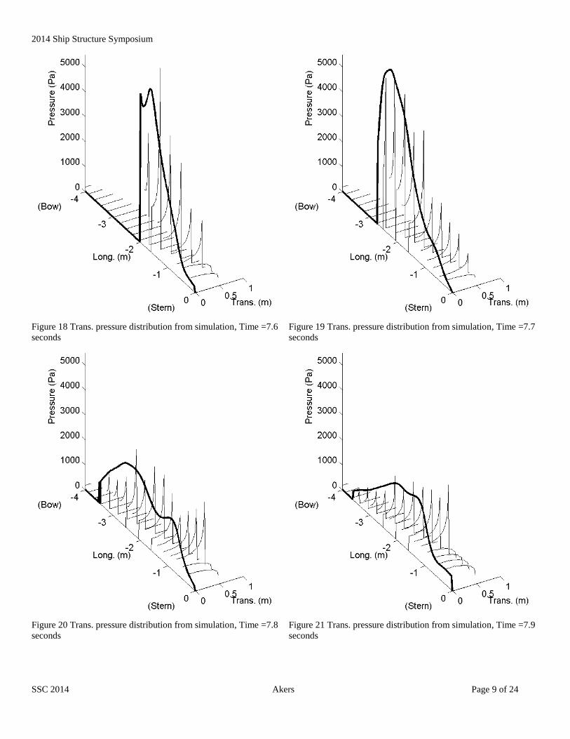
A set of hull pressures were calculated by the simulator at 0.1

second time steps starting at Time=7.0 seconds to Time=8.0

seconds. The hull pressures obtained from simulation using the

method presented in this paper are shown Figure 12 through

Figure 22.

Each hull pressure distribution was exported from the

simulation program into a text file containing

coordinate/pressure pairs. A load mapping program was used to

interpolate between simulator vertices and FEA vertices. Finally

the load mapping program was used to allocate pressure loads to

the S4 quad elements in the CalculiX model. The CalculiX FEA

program (Wittig, 2013) was used to estimate the Von Mises

stress in the aluminum hull panel and the results are included

here as Figure 23 through Figure 31. In these figures the bow is

on the left side of the panel and the stern on the right. At time

0.74 seconds the panel is barely wet, so the strain indicated by

the FEA program is uniformly 0 except for a small point near

the keel (see Figure 27). The panel is completely dry at time

steps 7.5 and 7.6, so only one strain figure is included for this

case (Figure 28).

The strain pattern shows relatively low, even strain when the

boat is between waves. As the boat crosses a wave the wetted

surface narrows and the pressure is concentrated near the keel,

finally disappearing when the panel is dry. When the panel

becomes wet at the next wave the high pressure from the chines-

dry region of operation appears near the keel and then spreads

out to cover the entire panel.

Figure 9 Mesh of fishing boat hull panel created using commercial meshing program.



Figure 10 Motion of aluminum fishing boat in regular waves (height=1.0 feet, wavelength=100 feet) predicted by simulation.

Figure 11 Accelerations on aluminum fishing boat predicted by simulation. Time series between 7 and 8 seconds were used for FEA.

Figure 12 Trans. pressure distribution from sim., Time =7.0 sec

Figure 13 Trans. pressure distribution from sim., Time =7.1 sec

-0.4

-0.2

0

0.2

0.4

0.6

0.8

2 3 4 5 6 7 8 9 10Time (sec)

Heave Loc (meters) Pitch (Degr /10) Wave Ht. at X=FP (meters)

-2

-1

0

1

2

3

4

5

6

2 3 4 5 6 7 8 9 10

Acc

ele

rati

on

(G's

)

Time (sec)

Heave Accel. (G's) Vert. Accel. at Fwd. Seat (G's)



Figure 14 Trans. pressure distribution from simulation, Time =7.2

seconds


seconds


seconds


seconds




seconds


seconds


seconds


seconds




seconds

Figure 23 Stress in panel, Time=7.0






Figure 27 Stress in panel, Time=7.4-7.6





of 24

VALIDATION

Test Case: Recreational Planing Boat To test the ability of the modified version of the simulator to

export accurate pressures, simulated results were compared with

pressure measurements taken on a ski boat built by Hydrodyne

Boat Company, in Fort Wayne, Indiana. The following

description of the boat is quoted from Royce (2001).

“[Hydrodyne Boat Company of Fort Wayne, IN] agreed to

build a modified 21 ft. long competition ski boat solely for the

purpose of gathering experimental data. The hull was made

using a production mold and the modifications were limited to

changes in the laminate schedule and outfitting of the boat.

“Hydrodyne’s standard construction consisted of a cored

laminate schedule in which E-glass roving and cloth was used

in conjunction with a balsa core. The balsa core was largely

omitted in favor of a ¼ inch thick layer of chopped strand

laminate, while the internal structure (longitudinal frames)

remained unchanged. Additionally, no pigment was used in

the protective gel coat layer which resulted in a translucent

hull that aided in the visual identification of the wetted foot

print from within the boat.

“The hull was outfitted with 200 through-hull manometer

taps in the port side bottom. During fitting out, the

arrangements and floor-boards for the port half of the hull

were excluded, allowing direct access to the manometer taps

and an un-obscured view for the visual identification of the

spray root location... The body plan view shows that the

deadrise varies from 47 degrees at the bow to 10 degrees at

the transom and a lifting strake at the chine runs the entire

length of the planing surface.”

Figure 32 Recreational ski boat from Hydrodyne. Translucent

hull makes location of manometer taps visible in this view.

Figure reproduced from Royce (2001).

A 3D CAD model of the Hydrodyne boat was built in

MultiSurf, and an IGES graphical file was exported for use in

the time domain simulator. The principle characteristics of the

test boat are listed in Table 1. Photos of the boat and locations

of the manometer pressure sensors are included as Figure 32 and

Figure 33.

Figure 33 Row of manometer taps in hull of Hydrodyne ski

boat. Figure reproduced from Royce (2001).

Geometric Model

Figure 34shows a 3D CAD model created in MultiSurf. In this

figure the keel flat can be seen in the green hull bottom. The red

surface is the chine flat. The MultiSurf CAD model was

modified to meet the needs of the simulator, and then was

exported as an IGES graphics file. The IGES file was read into

the simulator and the results are illustrated by Figure 35 and

Figure 36.

Table 1 Principal characteristics of Hydrodyne test boat.

LOA 20.5 ft. Displacement 2780 lbs.

LWL 18.0 ft. Chine Beam 5.7 ft.

LCG 6.5 ft. Shaft Angle 15.8 degrees

VCG 1.4 ft. Shaft Depth 1.0 ft.

Test Program, Quasi-Static Results

To compare the results of the simulator-based pressure

calculation with measured data, the Hydrodyne model was

simulated at a constant speed of 20 mph in fresh water with a

fixed trim angle of 3.07 degrees. The model was loaded to a

weight of 2,780 lbs. to match the Royce measurements. The

model was allowed to be free in heave. The simulator predicted

a slightly smaller draft than was reported by Royce, but this

comparison is difficult because it was unclear exactly how the

draft was measured on the real boat.

Figure 34 MultiSurf rendering of Hydrodyne

recreational boat



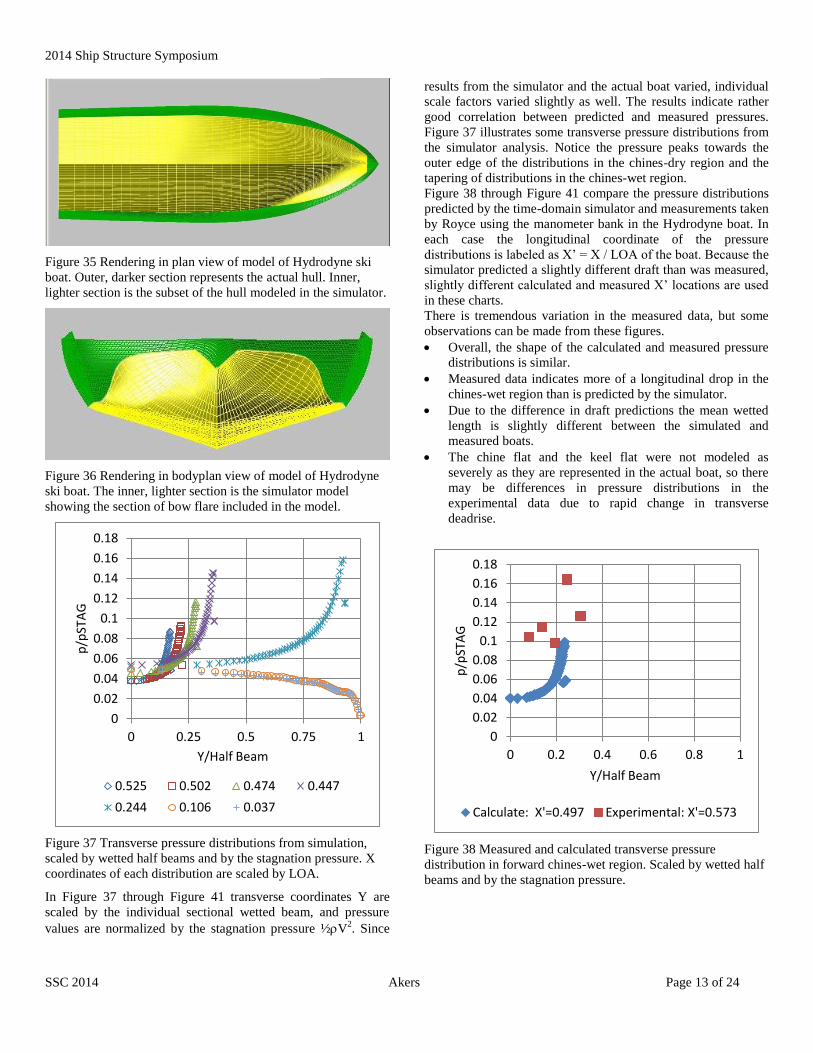
Figure 35 Rendering in plan view of model of Hydrodyne ski

boat. Outer, darker section represents the actual hull. Inner,

lighter section is the subset of the hull modeled in the simulator.

Figure 36 Rendering in bodyplan view of model of Hydrodyne

ski boat. The inner, lighter section is the simulator model

showing the section of bow flare included in the model.

Figure 37 Transverse pressure distributions from simulation,

scaled by wetted half beams and by the stagnation pressure. X

coordinates of each distribution are scaled by LOA.

In Figure 37 through Figure 41 transverse coordinates Y are

scaled by the individual sectional wetted beam, and pressure

values are normalized by the stagnation pressure ½V2. Since

results from the simulator and the actual boat varied, individual

scale factors varied slightly as well. The results indicate rather

good correlation between predicted and measured pressures.

Figure 37 illustrates some transverse pressure distributions from

the simulator analysis. Notice the pressure peaks towards the

outer edge of the distributions in the chines-dry region and the

tapering of distributions in the chines-wet region.

Figure 38 through Figure 41 compare the pressure distributions

predicted by the time-domain simulator and measurements taken

by Royce using the manometer bank in the Hydrodyne boat. In

each case the longitudinal coordinate of the pressure

distributions is labeled as X’ = X / LOA of the boat. Because the

simulator predicted a slightly different draft than was measured,

slightly different calculated and measured X’ locations are used

in these charts.

There is tremendous variation in the measured data, but some

observations can be made from these figures.

Overall, the shape of the calculated and measured pressure

distributions is similar.

Measured data indicates more of a longitudinal drop in the

chines-wet region than is predicted by the simulator.

Due to the difference in draft predictions the mean wetted

length is slightly different between the simulated and

measured boats.

The chine flat and the keel flat were not modeled as

severely as they are represented in the actual boat, so there

may be differences in pressure distributions in the

experimental data due to rapid change in transverse

deadrise.

Figure 38 Measured and calculated transverse pressure

distribution in forward chines-wet region. Scaled by wetted half

beams and by the stagnation pressure.

0

0.02

0.04

0.06

0.08

0.1

0.12

0.14

0.16

0.18

0 0.25 0.5 0.75 1

p/p

STA

G

Y/Half Beam

0.525 0.502 0.474 0.447

0.244 0.106 0.037

0

0.02

0.04

0.06

0.08

0.1

0.12

0.14

0.16

0.18

0 0.2 0.4 0.6 0.8 1

p/p

STA

G

Y/Half Beam

Calculate: X'=0.497 Experimental: X'=0.573




distribution in chines-wet region. Scaled by wetted half beams

and by the stagnation pressure.


distribution aftward in the chines-wet region. Scaled by wetted

half beams and by the stagnation pressure.


distribution chines-dry region. Scaled by wetted half beams and

by the stagnation pressure.

CONCLUSIONS A method has been demonstrated for predicting the motions of a

planing boat and for calculating the hull pressure distributions

associated with the motions. The pressure distributions can be

incorporated into a finite element program and used to predict

the strain in the hull materials.

Future enhancements to the algorithms described here include

better modeling of transverse flow separation, especially in hulls

with significant spray rails and multiple chines. The existing

implementation is limited to gradual changes in transverse

deadrise due to the necessity for smooth geometric derivatives.

Opportunities for additional research include the effects of

irregular seas and of oblique headings relative to the waves.

The finite element analyses were very rapid and offer the

intriguing opportunity to more closely couple the simulator and

the finite element solver for tasks such as optimization and long-

term fatigue analyses.

ACKNOWLEDGEMENTS This work was supported in part by Ship Structure Committee

Project SR-1470.

REFERENCES ABS (American Bureau of Shipping). RULES FOR

BUILDING AND CLASSING HIGH-SPEED NAVAL

CRAFT, American Bureau of Shipping, Houston, TX,

2013 (downloaded from "http://www.eagle.org" 12-

Feb-2014).

Akers, Richard H. “Dynamic Analysis of Planing Hulls in

the Vertical Plane,” Presented to Society of Naval

Architects and Marine Engineers, New England

Section, April 29, 1999a.

0

0.02

0.04

0.06

0.08

0.1

0.12

0.14

0.16

0.18

0 0.2 0.4 0.6 0.8 1

p/p

STA

G

Y/Half Beam


0

0.05

0.1

0.15

0.2

0.25

0.3

0 0.2 0.4 0.6 0.8 1

p/p

STA

G

Y/Half Beam


0

0.01

0.02

0.03

0.04

0.05

0.06

0 0.2 0.4 0.6 0.8 1

p/p

STA

G

Y/Half Beam




Akers, Richard H., Hoeckley, Stephen A., Peterson, Ronald

S., and Troesch, Armin W. “Predicted vs.

MeasuredVertical-Plane Dynamics of a Planing Boat,”

5th Int. Conf. on Fast Sea Transportation FAST,

1999b.

Broglia, R., A. Iafrati, A. "Hydrodynamics of Planing Hulls

in Asymmetric Conditions," 28th Symposium on Naval

Hydrodynamics, Pasadena, California, 12-17

September 2010.

Ensign, W., Hodgdon, J. A., Prusaczyk, W. K., Shapiro, D.,

and Lipton, M. "A Survey of Self-Reported Injuries

among Special Boat Operators," Report No. 00-48,

Naval Health Research Center, San Diego, CA, Nov.

2000.

Fridsma, Gerard. A Systematic study of the Rough Water

Performance of Planing Boats (Irregular Waves -- Part

II). Report 11495, Davidson Laboratory, Stevens

Institute of Technology, Hoboken, New Jersey, 1971.

Garme K. Time-domain model for high-speed vessels in

head seas [Thesis]. KTH, Department of Vehicle

Engineering; 2000.

Heller, S. R. Jr., and Jasper, N. H. "On the Structural

Design of Planing Craft," Quarterly Transactions of

the Royal Institution of Naval Architects, July, 1960.

IGES, Initial Graphics Exchange Specification, IGES 5.3,

U.S. Product Data Association, N. Charleston, SC,

1997.

IGES/PDES Organization (September 23, 1996), Initial

Graphics Exchange Specification: IGES 5.3, N.

Charleston, SC: U.S. Product Data Association,

"Formerly an ANSI Standard September 23, 1996 –

September 2006".

Kapryan, W. J., Boyd, Jr., G. M. Hydrodynamic Pressure

Distributions Obtained During a Planing Investigation

of Five Related Prismatic Surfaces, National Advisory

Committee For Aeronautics, Technical Note 3477,

Langley Aeronautical Laboratory, Langley Field, VA,

September 1955.

Korvin-Kroukovsky, B. V., and Chabrow, Faye R.: The

Discontinuous Fluid Flow past an Immersed Wedge.

Preprint No. 169, S.M.F. Fund Paper, Inst. Aero. Sci.

(Rep. No. 334, Project No. NR 062-012, ONR, Exp.

Towing Tank, Stevens Inst. Tech.), Oct. 1948.

Martin, M., Theoretical Predictions of Motions of High-

Speed Planing Boats in Waves. David W. Taylor Naval

Ship Research and Development Center,

DTNSRDC#76/0069, 1976.

Pierson, John D.: On the Pressure Distribution for a Wedge

Penetrating a Fluid Surface. Preprint No. 167, S.M.F.

Fund Paper, Inst. Aero. Sci. (Rep. No. 336, Project No.

NR 062-012, ONR. Exp. Towing Tank, Stevens Inst.

Tech.), June 1948.

Pierson, John D., and Leshnover, Samuel: A Study of the

Flow, Pressures, and Loads Pertaining to Prismatic

Vee-Planing Surfaces. S.M.F. Fund Paper No. FF-2,

Inst. Aero. Sci. (Rep. No. 382, Project No. NR 062-

012, ONR Exp. Towing Tank, Stevens Inst. Tech.),

May 1950.

Rosén, A. “Loads and Responses for Planing Craft in

Waves”, PhD Thesis, TRITA-AVE 2004:47, ISBN 91-

7283-936-8, Division of Naval Systems, KTH,

Stockholm, Sweden, 2004.

Royce, Richard. Thesis: “2-D Impact Theory Extended to

Planing Craft with Experimental Comparisons,”

University of Michigan, August 2001.

Savitsky, D. "Hydrodynamic Design of Planing Hulls,"

Marine Technology, 1, 1, pp. 71-95, 1964.

Shuford, Charles L., Jr., “A Theoretical and Experimental

Study of Planing Surfaces Including Effects of Cross

Section and Plan Form,” NACA Report-1355; 1958.

Smiley, Robert F.: A Semiempirical Procedure for

Computing the Water Pressure Distribution on Flat and

V-Bottom Prismatic Surfaces During Impact Or

Planing. NACA TN 2583, Langley Aeronautical

Laboratory, Washington, DC, December 1951.

Spencer, John. "Structural Design of Crewboats," Marine

Technology, 12, 3, pp. 267-274, 1975.

Stone, Kevin F., P.E. Comparative Structural Requirements

for High Speed Craft, Report Number SSC-439, Ship

Structure Committee, Washington, DC, February 2005.

Tveitnes, T., Fairlie-Clarke, A.C. and Varyani, K. "An

experimental investigation into the constant velocity

water entry of wedge-shaped sections," Ocean

Engineering, 35:14-15, 1463-1478, 2008.

USCG. Structural Plan Review Guidelines for Aluminum

Small Passenger Vessel, Navigation and Vessel

Inspection Circular No. 11-80. U. S. Coast Guard,

Washington, D.C., 1980.

Von Karman, T., The Impact on Seaplane Floats during

Landing,” National Advisory Committee for

Aeronautics (NACA), TN-321, Washington, DC, 1929.

Vorus, William S., "A Flat Cylinder Theory for Vessel

Impact and Steady Planing Resistance". Journal of

Ship Research, Vol. 40(2), pp 89-106, 1996.

Wagner H., Uber Stoss-und Gleitvorgange an der

Oberflache von Flussigkeiten. Z. angew. Math.

Mech.;12(4):193–215, 1932.

Wittig, Klaus; CalculiX USER’S MANUAL, Version 2.6,

July 6, 2013, [downloaded from

http://www.dhondt.de/cgx_2.6.1.pdf, 26-Jan-2014].

Zarnick, Ernest E. “A Nonlinear Mathematical Model of

Motions of a Planing Boat in Regular Waves”. David

W. Taylor Naval Ship R & D Center, DTNSRDC-

78/032, 1978.

APPENDIX 1: PLANING HULL TIME-

DOMAIN SIMULATOR

Overview of Simulator System Zarnick (1978) described a low-aspect ratio strip theory that can

be used to predict the vertical-plane motions of planing craft.

http://www.dhondt.de/cgx_2.6.1.pdf



The theory described in Zarnick's paper is the basis for the

simulator program used in this project.

Capabilities of Planing Boat Simulator

To support metocean data from a wide variety of courses, the

simulator can synthesize regular and irregular seas according to

Pierson-Moskowitz, JONSWAP, ITTC and Ochi 6-Parameter

spectra. Thrust is applied through a thrust vector, typically the

propeller shaft, or at the center of gravity.

Post-processing capabilities include Fourier transforms and

spectral density functions of motions, statistical summaries of

motions, motion-sickness dosage values, and Static Effective

Dosage (SED) per ISO 2651.

Calculating Forces and Moments; Simulating Motion

At each time step the time-domain simulator calculates sectional

pressure contributions from the following sources:

Impacting wedge (low aspect ratio strip theory)

2D ideal flow to model buttock flow. Results from panel

code are adjusted for extremely low aspect ratios.

Crossflow drag for sections in the chines-wet region

Viscous drag with a drag coefficient based on the mean

wetted length

Hydrostatic buoyancy

The results are weighted and added together on a section-by-

section basis to calculate an array sectional force vectors.

At each time step, the simulator:

1. Calculates the force vector and moment vector

contributed by each station

2. Calculates the added mass contributed by each station

3. Integrates the station force and moment vectors over the

entire hull to find the total force vector and moment

vector

4. Integrates the added mass over the entire hull to find the

total added mass and added pitch inertia

5. Solves the equations of motion to find instantaneous

angular and radial accelerations:

|A| = (|M| + |Added M|)-1

* |Total Force/Moment|

6. Integrates the accelerations to find velocities and the

velocities/angular rates to find positions/angles

The sectional force and moment vectors calculated in Step 1 are

the basis for calculating the vector forces exported to FEA.

Geometry Algorithms The geometry kernel in the planing hull simulator is critical.

Surfaces must be smooth and continuous, and it must be

possible to compute surface coordinates at any point on the

surface. Recognizing that the IGES 5.3 specification (IGES,

1997; IGES/PDES, 2006) describes most curve and surface

types used in CAD tools, the IGES specification was used as the

basis for the geometric kernel. Most of the geometric entities in

the specification are supported in the geometry kernel including

points, curves and surfaces. The CAD human interface supports

includes provisions for creating and editing points, lines,

parametric curves and ruled surfaces. Boat hulls may be defined

using BSpline surfaces, NURBS surfaces, surfaces of rotation,

and other IGES entities, but these must be created outside of the

simulator environment and imported into the simulator.

A mesh consisting of a list of hydrodynamic sections and

hydrodynamic buttock lines is derived from the geometric

entities that define the hull. These lines are created by:

Finding the intersection points of station and buttock planes

with all of the hull entities,

Adjusting the intersection points so that the order of points is

monotonic and the deadrise is between 0 and 90 degrees.

The points in the sorted point set become the vertices for

piecewise-linear stations and buttock lines. If the user specifies

reasonable resolution values then the accuracy of the results

rivals the accuracy of direct calculations of each vertex.

The heart of the planing hull simulator system is a geometry

program module that manages geometric entities, updates any

dependencies when one of the entities is modified, and allows

geometric operations such as calculating distances, intersections

and areas based on the entities.

Each surface in the simulator is defined by a set of polynomials

based on u and v:

X = fX(u, v)

Y= fY(u, v)

Z = fZ(u, v)

When the simulator updates the surface internally, it steps u and

v, calculating (X, Y, Z) vertices at each step. Surfaces thus are

defined by triangles connecting the nearest vertices. This is a

simple form of tessellation, a common practice in CAD

software. In Figure 42 dark green, straight lines (roughly

vertical) represent constant U- and V-parameter lines on a

parametric (e.g. BSpline) surface. The surface is broken into

triangles by finding an array of vertices located in the surface,

and then connecting the vertices with lines. Intersection lines

(stations, waterlines and buttock lines) are found by computing

the intersections between the triangle edges and the cutting

planes.

Figure 42 Tessellating a surface

Force Algorithms in the Simulator POWERSEA calculates five different forces acting on the hull

and uses a weighted sum to calculate overall forces and

moments to use in the equations of motion (refer to Figure 43):

Buoyancy

Impacting Wedge in Chines-Dry Region

Crossflow Drag in Chines-Wet Region



Viscous Drag

Dynamic lift due to Buttock Flow

Nomenclature

Var. Definition A Acceleration vector, inertial coords.

Sectional aspect ratio b Sectional wetted beam

Half wetted beam with respect to calm water Half wetted beam with pile-up water

A Added mass matrix (surge, heave, pitch) Sectional wetted beam Crossflow drag coefficient (chines-wet region)

Friction coefficient calculated from Mean Wetted Length using Prandtl-Schlichting line

Added mass coefficient

Added mass coefficient including pileup factor

Sectional pressure coefficient corrected for aspect ratio

Sectional pressure coeff. from buttock flow

Sectional drag force from buttock flow Sectional crossflow lift (normal to baseline) Sectional friction drag

Panel force from buttock flow at given section

Sectional wetted girth

Pitch moment of inertia of boat

Total added pitch inertia of boat ka Added mass coefficient Buttock length Sectional lift force from buttock flow M Total mass of boat Total added mass of boat Sectional added mass

(Added mass theory) particle of water moving at velocity vi

(Added mass theory) apparent mass of water moving with plate

Wetted draft of section (including pileup)

Thrust vector, x and z components (inertial)

U, V Horiz. and vertical velocity in boat coordinates

Surge velocity for buttock flow Sectional velocity in boat coordinates

Vertical speed of plate

Var. Definition

WF Wetting factor that relates calm water beam to fully wetted beam

wX Horiz. component of the wave orbital velocity, inertial cords.

State variable vector

X, Z Horiz and vertical coords. in inertial coordinates. +X forward, +Z down

Loc. of Center of Gravity of boat, Inertial coords.

Moment arm for thrust (propulsion) vector Global deadrise of wedge or section (radians)

Boat pitch angle (radians).

Density of water

Horiz. and vertical coords. in boat coordinate system

Impacting Wedge (Low Aspect Ratio Strip Theory)

Zarnick (1978) formulated a mathematical model of forces

acting on a planing craft. His method assumes that wavelengths

will be large with respect to the craft's length and that wave

slopes will be small. Following the work of Martin (1976),

Zarnick developed a mathematical formulation for the

instantaneous forces on a planing craft by modeling it as a series

of strips or impacting wedges. Zarnick derived the normal

hydrodynamic force per unit length as:

(11)

Where

(12)

Zarnick modeled sectional added mass as an impacting wedge:

(13)

where ka is an empirical added mass coefficient.

Zarnick used the value ka = 1.0 from the derivation of Wagner

(1932). The horizontal component wX of the wave orbital

velocity is considered small with respect to so only the

vertical component wZ is included. The boat relative velocities

with the vertical wave component included are:

(14)

(15)

A summary of the forces acting on the planing craft is:

(16)

(17)

(18)

(19)

Hydrostatic forces and moments must be included in the

analysis, but are difficult to predict. Water rise at the bow of a

CGx



planing vessel increases hydrostatic lift, flow separation at the

stern decreases hydrostatic lift, and both cause an increase in

pitching moment. These effects are speed dependent, and there

is no single factor that can be used to correct the hydrostatics

calculations for flow separation. In his work on rectangular

planing surfaces, Shuford (1958) suggested that hydrostatic

buoyancy should be halved in a dynamic simulation in order to

achieve the correct total lift force, and Zarnick used an

additional factor of one-half for the hydrostatic moment resulted

in an accurate trim angle. In Equation 17 and Equation 19

coefficients CBF and CBM correct the vertical force and pitching

moment. Zarnick set these coefficients to 0.5 based upon the

recommendation of Shuford.

The time derivatives and partial derivatives of the boat-

coordinate velocities are:

(20)

(21)

(22)

The vertical component of the wave orbital velocity can be

described by:

(23)

So

(24)

Making these substitutions and simplifying yields:

(25)

Combining terms yields:

(26)

The acceleration terms are estimated using a

numerical technique based on a running interpolation-

polynomial estimate of state variable derivatives. The term

is calculated using numerical derivatives.

Combining all terms into a single integral over the boat length

L, a sectional hydrodynamic normal force can be calculated as:

(27)

The total normal force is

. A similar analysis is

used to obtain an estimate of the instantaneous pitching

moment.

Wetting Factor and Added Mass

POWERSEA combines semi-empirical algorithms to predict

instantaneous forces and motions on a planing craft operating in

irregular waves. By adding the force components and

multiplying by the inverse of the sum of the inertial masses and

the instantaneous added mass of the water, it is possible to

predict the accelerations of the boat in three degrees of freedom.

Integrating the accelerations produces the velocities (rates), and

integrating again produces the time-dependent positions

(angles).

The term “added mass” describes a fictional amount of fluid that

moves synchronously with the movements of another object

submerged in the fluid. In reality there is not a single volume of

water that moves at the same rate as the object, adding to the

apparent mass of the object, but rather a large mass of fluid

particles that are set in motion at various speeds by the moving

object. The aggregate hydrodynamic force applied to the object

by these particles moving in their own trajectories can be

expressed in terms of a fixed (smaller) mass that is moving

exactly as the object moves. A two-dimensional flat plate

oscillating at very high frequencies in an ideal fluid will cause a

momentum change in the fluid such that the total derivative of

the momentum change will appear to be caused by a constant

mass moving in the same way as the plate. This effective mass

will appear to equal that of a cylinder centered on the plate:

(28)

The amount of fluid that moves with a plate with non-zero

thickness can be shown to be less than that associated with a



thin flat plate. POWERSEA calculates the added mass of a boat

planing on the surface, so only one-half of the cylinder is used

as the basis for the added mass. The sectional added mass is the

mass of a semicircle centered below the station:

(29)

Figure 43 Force components in planing hull simulator

The sectional added mass is the effective amount of water

moving under the impacting wedge as it penetrates the surface.

An added mass coefficient cmy is defined as a function of

deadrise.

mA = Cmy * /2 * * bHCalm 2 (30)

Cmy = Ka / WF2

Ka = f()

From impacting wedge theory the forces on the Chines-Dry

region of a planing craft arise from the change in momentum of

the added mass of water associated with each section. This force

is described mathematically as:

(31)

Where “D/Dt” is the substantial derivative operator acting on

the momentum :

This represents the force from successively deeper sections of

the boat as it passes in front of a stationary observer. The

velocity v is the vertical component of the velocity impacting on

the hull (in boat-coordinates), and the mass m is the added mass

of the water moving with the hull. In quasi-static planing

operation (steady-state, no waves, constant heave, pitch and

surge velocity), the added mass increases as the hull sections

plunge successively deeper in the water, while the impacting

rate of successive sections is constant.

Figure 44 Water pile-up and transverse jets cause wetted-beam

to be larger than static beam.

Figure 45 As a V-bottomed planing boat passes through the

water, the water piles up transversely along the hull bottom

Von Karman developed an expression for the added mass under

an impacting wedge (Von Karman, 1929) based on a semicircle

under the projected calm-water beam of the wedge:

(32)

(33)

Wagner modified von Karman’s solution by accounting for the

effect of water pile-up on the edges of the wedge as it enters the

water (Wagner, 1932):

(34)

(35)

-1200

-1000

-800

-600

-400

-200

0

0 1 2 3

Lift

Fo

rce

(N, p

osi

tive

do

wn

)

Distance Fwd. from Stern (m)

Buoy Lift Impact Wedge

Buttock Flow Crossflow Drag

Stern Bow

Static Wetted

Beam

(calm water)

Dynamic Wetted

Beam (with Pileup)

PLANING BOAT

Water

line

“Jet” (Water Pile-up)

High Frequency Added Mass

around a 2D flat plate.

mA= r2

High Frequency Added

Mass around a 2D flat

plate with deadrise.

mA = ka*r2



(36)

In the formulation in Equation 36 the wetting factor is

.

is a

non-dimensional factor defined as the ratio of the theoretical

added mass to von Karman's added mass (which is the

semicircle below the calm water projection). The added mass

coefficient for Wagner’s formulation is:

(37)

A wetting factor (WF) is defined as the ratio of the dynamic

wetted beam and the static (zero speed) wetted beam. The

wetting factor is a non-linear function of the global deadrise .

Zarnick assumed that the water pileup factor was /2 so that the

depth of penetration is:

(38)

Tveitnes, et al. (2008) investigated the water rise from

impacting wedges and compared fomulations from Band, Vorus

and Zhao. Vorus developed a robust model for the wetting

factor (Vorus, 1996) and his work was used as the basis for the

wetting factor model in POWERSEA. Data calculated using

Vorus’s method was fit to a quadratic regression model of the

form:

(39)

Where d1, d2, and d3 are regression coefficients. The coefficients

for this model are listed in Table 2. Data points calculated using

Vorus’s model and a curve calculated from the regression

model used in the simulator are included in Figure 46.

Figure 46 Wetting Factor (Dynamic Wetted Beam vs Static

Wetted Beam)

Table 2 Regression coefficients for wetting factor model

Coefficient Value

d1 1.56528

d2 -0.64721

d3 0.14048

Using this empirical formula, the wetted beam of a wedge with

a constant vertical velocity is

(40)

The literature describes two different added mass factors, Cm'

and Cmy. is a vertical added mass factor which is defined as

. An empirical added mass coefficient is

defined to fit measured data and Cmy is redefined as:

(41)

Zarnick (1978) modeled the added mass of a section as a

semicircle whose width is the “wetted beam” of the section. In

the present formulation Zarnick’s wetting factor of

was

replaced with the empirical wetting factor WF:

(42)

The algorithm for modeling added mass in the simulator starts

by calculating the wetted beam, which is then used along with

Cm' to calculate instantaneous sectional added mass.

Figure 47 Added Mass coefficient versus deadrise

The relationships between several added mass formulations are

shown in Figure 46. From the literature a common factor in

added mass coefficient formulations is the basis function:

(43)

This function was used as the basis for regression models of the

Savander and Vorus formulations. As can be seen in Figure 47,

the numerical approximations are quite close to formulations of

Vorus and Savander. The planing hull simulator models the

added mass coefficient Ka with an empirical model. The

derivative of the added mass coefficient with respect to deadrise

is a closed form expression calculated directly from the

regression models of the Vorus/Savander formulations.

1.2

1.3

1.4

1.5

1.6

1.7

1.8

0 5 10 15 20 25 30

We

ttin

g Fa

cto

r (w

etF

acto

r)

Deadrise (degrees)

Model Test Data

Band Model

Zhao Model

Vorus Model

Vorus Model, Curve Fit

0

0.2

0.4

0.6

0.8

1

1.2

1.4

0 10 20 30 40 50 60

Ad

ded

Mas

s C

oef

fici

ent,

Cm

'

Deadrise, Beta

Savander Cm'

Vorus Cm'

Savander Cm' (curve fit)

Vorus Cm' (curve fit)



Figure 48 Simulator precalculates geometric properties at each

section. Properties are based on wetted area which includes

water pileup.

Figure 49 Precalculated geometric properties at each section

For computational efficiency (Figure 48, Figure 49), the

simulator precalculates the values of static wetted beam bHCalm

and dynamic wetted beam bHPileup versus submergence (draft),

and creates spline models of the relationships. During each

iteration in a time-domain simulation, the simulator finds the

derivatives of bH with respect to draft by differentiating the

spline functions created for each section.

To calculate the substantial derivative of the sectional

momentum it is necessary to calculate the time derivative of the

sectional added mass:

(44)

(45)

(46)

(47)

A station is described by a piecewise linear curve connecting

vertices that are found during the meshing operation. The global

deadrise of a station is defined as the arctangent of the slope of

the submerged portion of the station,

, where

tPileup is the draft of the section including the piled up transverse

jet. The time-derivative of deadrise at a station is calculated as:

(48)

(49)

(50)

(51)

The terms

are calculated from the empirical models

and

is estimated at every time step in the simulation.

Buoyancy

The planing hull simulator is intended to simulate high speed

craft so the majority of the lift force arises from hydrodynamic

mechanisms. Hydrostatic forces cannot be ignored, however,

especially at lower planing speeds. In reality the hydrostatics

and hydrodynamic forces cannot be separated, but for planing

boats it is possible to make some simplifying assumptions about

the hydrostatic forces and treat them separately from the

hydrodynamic ones.

0

0.1

0.2

0.3

0.4

0.5

0.6

0.7

0 1 2 3

Distance Fwd. from Stern (m)

Half Beam Half Girth Half Area

Stern Bow

-0.2

-0.1

0

0.1

0.2

0.3

0 1 2 3Distance Fwd. from Stern (m)

Global Deadrise) Centroid Z Coord

Keel Submergence Chine Submergence

Stern Bow



For most planing boats the water will separate off the bottom

edge of the transom, so the wetted surface is not bow-stern

symmetric. This effect is considered to be part of the impacting

wedge formulation, so no hydrostatic “drag” is included in the

simulator force formulation.

As illustrated in Figure 50, this choice results in a lower

hydrostatic bow-down moment than would be obtained by using

the calm water surface as the reference plane.

Engineers calculate hydrostatic pressure by applying the

Bernoulli Equation along a streamline starting at the free surface

and ending at the point of interest. In the case of a planing craft,

different results are obtained if the calm water surface is used as

the starting point (Figure 50, A) than if the wetted surface at the

boat hull is used as the starting point (Figure 50, B).

Figure 50 Calculating Displacement using calm waterline (top,

A) or dynamic waterline (bottom, B). Buoyancy creates a larger

bow-up moment in B than in A.

By comparing simulation results for quasi-static (constant

speed) operation, it was found that more accurate results are

obtained using the pile-up wetted surface on the boat hull as the

zero-pressure reference height for hydrostatic pressure

calculations.

The hydrostatic forces on the planing boat are not fore-aft

symmetric as the transom is dry when the boat is on plane. This

factor should be taken into account to calculate surge resistance

accurately.

Viscous Drag

Special attention is paid to the friction force FD. At each time

step the mean wetted length, the Reynolds Number, and a

friction coefficient can be calculated. The friction coefficient is

calculated using the Prandtl-Schlichting line. For most of the

hull this friction coefficient will be valid, but for highly curved

sections the water flow will be significantly greater than the

nominal water flow past the hull. A sectional friction force is

calculated as:

(52)

Crossflow Drag

The impacting wedge algorithm does not apply to the chines-

wet region because it depends on the substantial derivative of

the water momentum, D(ma*v)/dt. Since the added mass ma

beneath the hull is a fixed value in the chines-wet region, a

different mechanism is required to model the dynamic force in

this region. The dynamic force is modeled in this region using a

drag coefficient, CDC, which varies along a straight line from

the start of the chines-wet-region to the transom. The sectional

lift from the crossflow drag is

(53)

A cosine blending function is applied starting at 1/4 beam

forward of the transom so that the CDC coefficient drops

smoothly to zero at the transom (Garme, 2000).

Buttock Flow

To better model dynamic lift and induced drag due to the flow

of water along the bottom of planing hulls, a 2D panel code was

added to the simulator. The simulator precalculates an array of

drag coefficients using a panel method. This array spans

multiple buttock locations, boat trim angles and buttock draft

angles. During each time-step, the sectional pressure coefficient

is calculated by using a quadratic interpolation between the

precalculated results.

A triangular mesh is generated from the hull geometry to

represent the hull surfaces. An array of 2D foils is created by

intersecting the submerged portion of the mesh (using the calm

water draft) along buttock planes starting from the centerplane

out to 98% of the maximum beam at the chine. The resulting

points are mirrored across the calm waterline and these are fitted

with a foil curve (Figure 51). Additional foil curves are

generated by generating buttock curves at the same buttock

planes but fractions of the calm water drafts.

Using a panel code derived from a constant-strength vortex

method described in Katz (1991), a matrix of pressure

coefficients is calculated at the x-coordinates of a set of

transverse sections along each buttock and at each draft for a

range of trim angles ranging from -30 degrees to +30 degrees.

These values are precalculated in a mesh operation that is

performed before any time-domain simulation runs.

Figure 51 Planing hull with foils created from buttock curves

At each time step of an analysis, a pressure coefficient (Cps0) is

calculated for each section. The pressure coefficient is obtained

by finding the instantaneous half-wetted beam, draft, and trim

angle of the section. Using these values the pressure coefficient

A

B



is interpolated from the matrix of coefficients

previously calculated.

In Figure 52 the pressure coefficients for buttock

lines are labeled by the fraction of the maximum

beam (e.g. “Buttock 0.400” is located at 40% of

BMax from centerplane).

A correction for low aspect ratio wings using

Jones’ approximation (Jones, 1946) is applied to

the pressure coefficient:

(54)

(55)

The panel force due to pressure at any given

section is calculated as:

(56)

Lift ( ) and drag ( )

forces are derived from this panel force and the

slope of the buttock curve at the given section angle of attack .

Combining Algorithms

The planing hull simulator calculates a number of force

components, but these force components are not independent

from each other. The forces must be blended in a rational

manner to avoid missing components or adding multiple models

for the same physical effect.

Although research in this area is ongoing, the following

algorithm is used to calculating linear weighting factors to

combine the forces:

1. Weighting factors must be based on non-dimensional

geometric characteristics, not on dynamic characteristics.

2. Weighting factors must be set and validated using model

test and full-scale test data.

3. Weighting factors are polynomial functions of the principal

characteristics of the model boat, but no term can have

more than two characteristic factors and no factor can have

an exponent outside the range of -2 to 2.

The first rule guarantees that the dynamics of the boat are a

function of the force algorithms and not of the weighting

factors. That is as the boat speed changes the hydrodynamics is

modeled in the force equations, not in the weighting

coefficients. The second rule helps to guarantee that the

weighting factors result in predictions that can be extrapolated

to new models for similar boats. The third rule helps to avoid

numerical oscillations between the peaks and troughs of

complex polynomial equations.

The results included in this report were accomplished with a

fixed set of weighting coefficients that have been found to

produce accurate results for a wide range of high-speed boats.

Solving Equations of Motion The acceleration terms can be factored out of the sectional force

and moment expressions:

={

}

(57)

={

}

(58)

Figure 52 Pressure coefficients on buttocks from panel code (4 degree trim)

0

0.1

0.2

0.3

0.4

0.5

0.6

0.7

0.8

0.9

1

0 20 40 60 80 100 120 140 160 180 200

Sect

ion

al P

ress

ure

Co

eff

icie

nt,

cp

Section Index

Buttock 0.000 Buttock 0.050 Buttock 0.100 Buttock 0.150 Buttock 0.200

Buttock 0.300 Buttock 0.400 Qtr Beam Buttock 0.500 Buttock 0.667 Buttock 0.833

BOW STERN



(59)

Combining the modified sectional force and moment

expressions with the general equations of motion yields:

(60)

A set of state variables are

chosen. The matrix equation above can be written as

where |A| is the mass matrix, is the derivative of the state

variable vector , and is the right-hand side

forcing function, which is itself a function of the state variables.

At each time step the matrix equation is solved for .

The resulting equations are integrated to find the new value of

the state variables , and the previous value of the

state variables are integrated to find the new value

of the state variables .

fxA

x

CGCGCG θ,z,x f

fAx1

a method of structural load prediction for high-speed ... craft loads.pdf · a method of structural...

Documents