a method for the prediction of detection ranges for pulsed
TRANSCRIPT
Scholars' Mine Scholars' Mine
Masters Theses Student Theses and Dissertations
1960
A method for the prediction of detection ranges for pulsed A method for the prediction of detection ranges for pulsed
doppler radar doppler radar
Phillip Orlan Brown
Follow this and additional works at: https://scholarsmine.mst.edu/masters_theses
Part of the Electrical and Computer Engineering Commons
Department: Department:
Recommended Citation Recommended Citation Brown, Phillip Orlan, "A method for the prediction of detection ranges for pulsed doppler radar" (1960). Masters Theses. 4178. https://scholarsmine.mst.edu/masters_theses/4178
This thesis is brought to you by Scholars' Mine, a service of the Missouri S&T Library and Learning Resources. This work is protected by U. S. Copyright Law. Unauthorized use including reproduction for redistribution requires the permission of the copyright holder. For more information, please contact [email protected].

A METHOD FOR THE PREDICTION OF
DETECTION RANGES FOR PULSED
DOPPLER RADAR
BY
PHILLIP ORLAN BROWN
A
THESIS
submitted to the faculty of the
SCHOOL OF MINES AND METALLURGY OF THE UNIVERSITY OF MISSOURI
in partial
Rolla, Missouri
1960

ACKNOWEOOEMENTS
The author wishes to acknowlege the guidance and
assistance of the following persons:
Doctor R. E. Nolte of the Missouri School of
Mines and Metallurgy,
Mr. H. W. Hamm and Mr. R. Dierberg of the
Electronics Guidance Group, McDonnell
Aircraft Corporation.
ii

CHAPTER
I.
II.
iii
TABLE OF CONTENTS
PAGE
THE PROBLEM AND DEFINITIONS OF TERMS USED ••• 1
The Problem •••• a a •••• a • • • • • • • • • • • • • • • • • • • • 2
Statement of the problem •••••a•aa••a•••• 2
Justification of the problem............ 2
Definitions Of Terms Used................. 2
Characteristic radar range . . . . . . . . . . . . . . Radar cross section . . . . . . . . . . . . . . . . . . . . . Detection criterion ••••••••••••••••saaa•
False-alarm time •••aa••a•ca•ca••o•••••••
Single-look probability ••••••••••••.••••
Cumulative probability ••••••••••••••••• a
BRIEF DESCRIPTION AND THEORY OF A PUIBED
DOPPI.ER RA.DAR • • • • • • • • a • • • • a • • a • • a • • • • • • • • • • •
Description And Operation Of A Pulsed
Doppler Radar . . . . . . . . . . . . . . . . . . . . . . . . . . .
2
3
4
4
4
5
6
7
Transmitted And Received Spectrums •••••••• 8
Transmitted spectrum •••a•••••••••a•a•••• 8
Received spectrum. •••••a•••••a••a••••a••• 9
Ground clutter ••••••••••••a••a••••a••· 10
Pulsed doppler spectrum. ••••a•••••a•••• 12
Su.mm.a ry • • • • a • • • • • • • • • • a • • • • • • a • • • • • • • • • • • • 14

CHAPI'ER
III
IV
v
SINGLE-SCAN DETECTION RANGE . . . . . . . . . . . . . . . . .
iv
PAGE
15
The Normalizing Range .••••••.••••.•••.•••• 15
Definition Of Detection And The Bias Level. 20
Threshold Level . . . . . . . . . . . . . . . . . . . . . . . . . Single-look probability .................
Signal-plus-noise ..................... Signal obscuring ••••••••••••..••••••••
Suntm.a ry . • • . a • • • • • • • • • • • • • • • • • • • • • • • • • • • • • •
CUMULATIVE DETECTION RANGE .••••.••..••••••••
Cumulative Probability . . . . . . . . . . . . . . . . . . . . Approximate solution . . . . . . . . . . . . . . . . . . . .
A Procedure For Detection Range
21
23
24
25
32
36
36
37
Computation............................. 37
Definition of symbols used . . . . . . . . . . . . . . Case
Case
I
II
. . . . . . . . . . . . . . . . . . . . . . . . . . . . . . . . . . .................................
Case III . . . . . . . . . . . . . . . . . . . . . . . . . . . . . . . .
39
40
43
44
Example problem . • • • • • • • . • • . • • . . • • . • • . • • • 45
Pulsed doppler radar parameters ..•.••. 46
Calculations . . . . . . . . . . . . . . . . . . . . . . . . . . Summary
CONCLUSIONS
.................................
......................... • ....... .
46
48
50
B IBLI OGRA..PI-IY . • . . • • • • • • • • • • • • • • • . • • . . . • . . • • . • . • • . • • • • . . 5 2
VITA • • . • • . • • • • . • • • . • • • . • • • • • . • • • • • • . • • • • • • . • • . • • • • . . • • 54

v
LIST OF FIGURES
FIGURE PAGE
Simplified Block Diagram of a Pulsed
Doppler Radar ••a•a•••aa••••aaaaaa•a••a•••D•• 7
2.
3.
4.
Frequency Spectrum of Transmitted Wave ••••aa
Ideal Receiver Spectrum of a CW Radar •••••••
Receiver Spectrum of a CW Radar ••a•a••••••••
5. Received Spectrum of a Pulsed Doppler
9
10
12
Radar •••••••• a •••••••••• a • • • • • • • • • • • • • • • • • • • 13
6. Block Diagram of One Detection Channel ••••••
7. Threshold Level as a Function of the Number
8 •
9.
10.
11.
of Variates Integrated and the False-Alarm
Probability . . . . . . . . . . . . . . . . . . . . . . . . . . . . . . . . . Single-Look Probability of Detection in
Terms of Normalized Range (Pfa = 10-5 ) ••••••
Single-Look Probability of Detection in
' ( -6) Terms of Normalized Range Pfa = 10 ••••••
Single-Look Probability of Detection in -7) Terms of Normalized Range (Pfa = 10 ••••••
True Detection Curve and Obscuring Effects ••
12. Average Single-Look Probability of Detection
20
26
27
28
29
31
in Terms of Normalized Range •••••••••••••••• 33

13. Value of the Integral of Equation 34 in
14.
15.
16.
17.
18.
Terms of Normalized Range •••••••••a•••••••••
Flight Geometry for Case I ••••a•a•··········
Flight Geometry for Case II ••a•a••••••••••••
Flight Geometry for Case III ••••••a•••••a•••
Flight Geometry for a Collison Course ••••a••
Cumulative Probability of Detection •••••••••
vi
38
41
43
45
46
49

TABLE
I
vii
LIST OF TABLES
PAGE
OBSCURED RANGE CORRECTION FOR SINGLE-
LOOK DETECTION RANGE • • • • • • • • • • • • • • • • • • • • • • • • • 3 4

CHAPTER I
THE PROBLEM AND DEFINITIONS OF TERMS USED
Modern radar systems must provide greater detection
ranges both against high and low altitude targets because of
the significant advances in weapon speed and range. Extended
range indicates that the power transmitted by the · radar must
be increased. It follows, that ground return becomes a pro
blem even at high altitudes.
There are at present three basic types of radars which
are (1) pulsed, (2) continuous wave, and (3) pulsed doppler
radar. The conventional pulsed radar now closely approaches
the theoretical optimum performance; however, it does not
have the inherent ability to distinguish between ground re
turn and moving targets. The continuous wave radar has the
ability to distinguish between fixed and moving targets but
does not retain the time form of the information and also
the continuous wave radar has practical difficulties which
limit the usefulness of this system in airborne applications.
The pulsed doppler radar detects the doppler frequency shift
of moving targets, as in the continuous wave radar, while
retaining the time form of the returned information as in
pulsed radar systems.
It is important to be able to evaluate and predict
the operation of a radar as well as the comparison of differ-

2
ent radars. Range performance and detection range capabilities
are methods by which radars are compared and their operation
predicted.
I • THE PROBLEM
Statement of the problem. It is the purpose of this
study to present a method for computing the range performance
of an air-interceptor pulsed doppler radar in terms of detec
tion ranges. The analysis of the detection range performance
includes target scintillation.
Justification of the problem. It is well established
that the prediction of radar range performance is of a
statistical nature. The literature on the analysis of pulsed
radar range performance is quite extensive, Marcum (1) (2),
Swerling (3), and Drukey (4). Few unclassified articles have
been published concerning the range performance of pulsed
doppler radar. That which has been published, Bussgang (5),
and Barlow (6), c-ontains only methods for non-scintillating
targets.
II. DEFINITIONS OF TERMS USED
Characteristic radar range. It is realized that the
range of a radar must be stated in terms of probabilities
rather than a specific quantity. The commonly accepted

3
definition of the characteristic range of a radar is: that
range at which the radar has a thirty-six point eight (36.8)
per cent probability of receiving a signal from a target of
given cross section. The target cross section is expressed
in terms of an average of its scintillating value and the
target is viewed from a partictular aspect angle.
The term •probability of receiving a signal" should
not be confused with the term "probability of detecting a
signal.• The latter term involves factors such as the number
of variates integrated, type of detection process, and the
detection tim.e.
Radar cross section. The characteristic range of a
radar is proportional to the radar cross section. The re
sults of this study are also dependent on this quantity as
the cumulative probability of detection is a function of the
target cross section. A formal definition of the radar cross
section is •4rr times the ratio of the power per unit solid
angle scattered back toward the transmitter, to the power
density (power per-unit area) in the wave incident on the
target,• Ridenour (7). The cross section of a target depends
not only on the wave length but also upon the angle from
which the target is viewed by the radar. This angle is usually
given the term •target aspect• angle. Only for certain cases
can the radar cross section be rigorously calculated; for
most targets it is inferred from radar data itself.

4
Detection criterion. There are as many criteria for
detection as there are methods of detection. This study has
involved electronic detection; therefore, only that defini
tion is given:i A signal is considered detected if tle output
of the post detector integrator exceeds a predetermined level.
This predetermined level is termed the threshold or bias
value.
False-alarm time. The false-alarm time of a radar
system measures the rate at which false-alarms, or noise
fluctuations that are interpreted as target echos occur.
There exist in the literature at least two different defini
tions of this time interval, Hollis (8).
Quite possibly the most common definition of false- .
alarm time is the average interval of time between false
target indications. The false-alarm time used by Marcum (2)
is defined as the time in which the probability is one-half
(1/2) that a false-alarm will not occur.
The difference in the false-alarm times as defined
in the previous paragraph is approximately forty-five (45)
per cent; however, the probabilities of one false-alarm
occuring within their respective alarm times differ by only
about six (6) per cent.
Single-look probability. The single-look probability
of detection is defined as the probability that a signal will
exceed the threshold value during one scan of the radar antenna.

Cumulative probability. The cumulative probability
of detection is defined as the probability that a target
starting at a range Rm will be detected at least once by
the time it reaches a range Rx.
5

CHAPTER II
BRIEF DESCRIPTION AND THEORY OF A PULSED DOPPLER RADAR
The natural phenomenon known as the doppler effect
6
can be found in such fields as sound, light, and radio waves.
The doppler effect has been known since 1842, when it was
first investigated by Christian Johann Doppler. However, it
was not until 1933, that the doppler effect in radio waves
was first investigated for a practical application of de-
termining an aircraft's ground velocity for use in naviga-
tional systems. Only within recent times has the doppler
effect been investigated as applicable to a pulsed doppler
detection system.
A pulsed doppler radar detects the doppler frequency
translation of moving targets, while the time form of the
information is retained. This system differs from other
systems· which use . the doppler effect, such as moving target
indicator radars, in that the actual frequency difference
of the transmitted and received frequencies is detected and
analysed a
It is the purpose of this chapter to review the prin
ciples of the doppler phenomenon with particular emphasis to
a pulsed doppler radar system located on a moving platform,
such as an aircraft. This review of doppler principles in

7
conjuction with a simplified hypothetical pulsed doppler
radar will illustrate the areas in which the prediction of
the range performance differs from that of pulse and con-
tinuous wave radars.
I. DESCRIPTION AND OPERATION OF A PULSED DOPPLER RADAR
A simplified block diagram, Maguire (9), of a pulsed
doppler radar is shown in Figure 1. The transmitter portion
basically consists of an r-f oscillator, a modulated power
amplifier, a pulser, and a duplexer comm.on to both the trans
mitter, and the receiver. The r-f oscillator continuously
drives the modulated power amplifier which is turned on and
off by the square wave from the pulser. The output of the
fo •
f +fg 0 ..
Modulated Duplexer ..... _...,. Power. Allp.
Mixer
Range ~ler Gate ere
Alarm Threshold DeTice
FIGURE 1
SIMPLIFIED BLOCK DIAGRAM OF
A PULSED DOPPLER RADAR
R-F O•cillator
Pulser
Detector

8
amplifier is a train of discontinuous sine (or cosine) waves
in a square wave envelope. The phases of the sine waves in
each successive pulse are identical and the transmitter out
put is coherent rather than random as in a pulsed radar.
The frequency of the returned radiation from a target echo
has been shifted from the transmitted frequency by an amount
fd called the doppler frequency.
The returned pulses, after amplification, are passed
through a range gate. A narrow band filter selects only the
central line from the pulse spectrum, thus converting the
return to a continuous wave signal. The signal is then appli
ed to a bank of narrow band-pass. filters covering the doppler
region of interest. Each doppler (band-pass) filter is follow
ed by a detector and a post detection integrator. The output
of the integrator is applied to a threshold device. If the
integrated output voltage exceeds the threshold, then an
alarm results which means a detection occures.
II. TRANSMITI'ED AND RECEIVED SPECTRUMS
Transmitted Spectrum
The frequency spectrum of a pulsed signal of duration
'l't which is transmitted at fixed intervals of time 1/fr is
represented by the Fourier series
00
G(t) = EP 'l'tf r ~sin TI -rtnf r
L_ 1T -i't nf r
(1)
n = -oo
where
EP - peak voltage of transmitted pulse.
1t - time duration of transmitted pulse.
f0
- carrier frequency of transmitter.
fr - pulse repetition frequency.
9
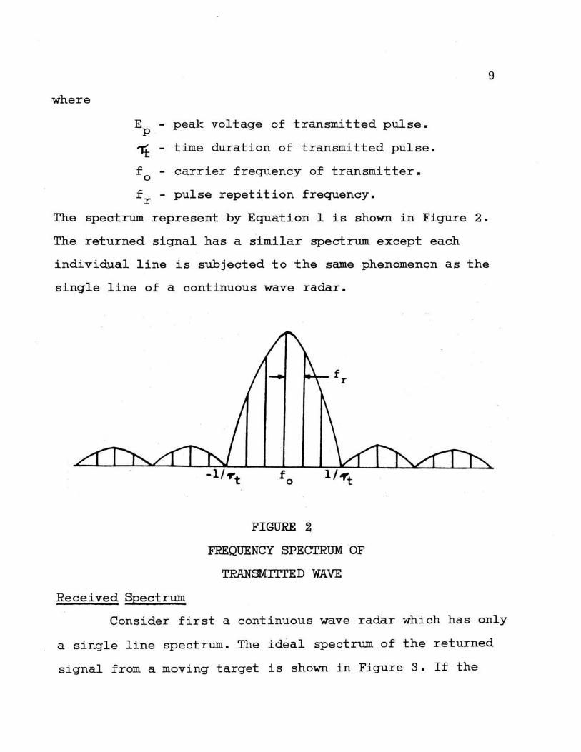
The spectrum represent by Equation 1 is shown in Figure 2.
The returned signal has a similar spectrum except each
individual line is subjected to the same phenomenon as the
single line of a continuous wave radar.
Received Spectrum
FIGURE 2
FREQUENCY SPECTRUM OF
TRANSMITI'ED WAVE
Consider first a continuous wave radar which has only
a single line spectrum. The ideal spectrum of the returned
signal from a moving target is shown in Figure 3. If the

(1) "O ~
+" ·.-4 .--..
l
E
-jfd-2VR .~ ~ I I
Tarqet I Echo
f fo+fd 0
FIGURE 3
IDEAL RECEIVER SPECTRUM
OF A CW RADAR
10
radial velocity between the radar and the target is VR, then
the doppler frequency shift is given by the equation
where
VR - relative (radial) velocity of the interceptor to the target.
A. - transmitted wavelength.
(2)
The derivation of Equation 2 is found in reference 10.
Additional doppler frequencies will appear in the returned
signal. These additional undesired signals are the result of
the aircraft moving with respect to the ground. The undesired
signals are called ground return or simply clutter.
Ground clutter. Individual irregularties on the
ground act as reflecting objects for the energy radiated

11
towards the ground. There exists a component of aircraft
velocity directed towards (or away) from these scatterers.
It is this velocity component in conjunction with the antenna
pattern of the radar that causes the returned energy to be
doppler translated, although the aircraft may not be approach-
ing or receding from the ground surface.
Ground clutter is caused by the main beam, side lobes,
and the minor lobes of the antenna pattern intersecting the
ground. Regardless of the altitude and the direction in
which the antenna main beam is pointing, ground clutter is
received from all directions. The doppler shift of the ground
return is expressed as
where
fd (clutter)= (2V1 /~) cos 8
v1 - interceptor velocity.
8 - angle between interceptor velocity vector and the direction of radar propagation.
(3)
The doppler shift · of the clutter varies continuously from
(-2V1 /~) to (+2V1 /~). The magnitude of the return at a
particular doppler frequency depends on the gain of the
antenna for that portion of the ground producing the doppler
frequency and the range of that sector of ground. The ex-
pression given is for a single forward-looking radar beam
which is suitable for motion of an aircraft in a plane. A
typical sketch of the clutter spectrum is shown in Figure 4.

Side Lobe
Altitude \ Line
Tarqet VEcho
+zv1 /).,, Frequency
FIGURE 4
RECEIVER SPECTRUM OF A CW RADAR
12
Pulsed doppler spectrum.. Each individual line of the
received spectrum of a pulsed doppler radar is subjected to
the same phenomenon as the single line of a CW radar. Figure
5 shows the spectrum appearing at the receiver of a pulsed
doppler radar. For simplicity only the central line and its
two adjacent lines are shown. In order to obtain maximum
range performance it is necessary to prevent a high closing
rate target echo from entering the side lobe clutter of the
first upper side band. This is accomplished by setting the
pulse repetition frequency high enough so that the side
bands are widely separated.
The maximum doppler shift of a target with velocity
VT is equal to 2(V1max + Vry11ax)/~; therefore, to prevent
clutter from obscuring the target echo it is necessary that
fr~ (4V1max + 2VTmax)/~. Values of pulse repetition

13
frequencies of 100,000 cycles-per-second are typical. The
necessity for a high pulse recurrence frequency results in
the range between transmitted pulses being less than the
desired maximum range. The target, therefore, appears several
times in the fundamental range interval. Special techniques
are used to determine the unambiguous range to the target.
A second consequence of the high repetition frequency
is the possible obscuring of the received signal, that is,
the signal_ returning when the receiver is gated off. A target
echo which is received near the maximum detection range of
the radar and being tracked to a minimum range passes through
the transmitter pulse a number of times.
/ I
I -I
/side I Lobe
/ /
,,,, /
/ / -
/
--------,,,,, ----...__ ',,
', Sin x ,, X -
Main Beaa
' --~ .. ' '
Tarqet Echo
FIGURE 5
RECEIVED SPECTRUM OF A
PULSED DOPPLER RADAR
- f +f o r
\ \ \ \ - \ -
\ \

14
Swnmary
The pulsed doppler radar combines the features of the
pulsed radar and the continuous wave radar. The use of high
pulse repetition frequencies permits the use of large duty
cycles thereby achieving high average power with low peak
powers. Clutter is discriminated against by exploiting the
coherence of the target echo.
Velocity ambiguities are prevented by selecting only
the central line of the returned spectrum. This filtering
reduces the signal power by the duty cycle of the signal.
In general, only a fraction of each received pulse is passed
by the range gate and. the signal · power is further reduced by
an obscuring factor e.

CHAPI'ER III
SINGLE-SCAN DETECTION RANGE
15
Chapter II illustrated the basic operation of a pulsed
doppler radara It was pointed out that only the central line
of the received spectrum is utilized in determining the pre
sence or absence of a target and that the signal power is
reduced by the filtering action of a narrow band filter.
Possible obscuring further reduces the signal power avail
able for detection.
It is the purpose of this chapter to account for the
effects of the previous paragraph on the characteristic radar
range of a pulsed doppler radar. The equation for the single
scan detection range is developed by analysing the detection
device. Much of the development is drawn from work previously
done by others in connection with pulsed and continuous wave
radars.
I. THE NORMALIZING RANGE
The ratio of the signal energy available for detection
to the competing noise (or clutter) energy is the fundamen
tal quantity of interest in the theory of radar detection.
In practice the physical quantity measured is power; there
fore, an analysis in terms of power rather than energy is
made. The "free space• radar range equation is derived in

reference (7) and is given as
where
PS = PtG~2o
(4.r)3 R4
Pt - peak transmitted power.
G - antenna gain one-way.
~ - transmitted wavelength.
a- - radar cross section of target.
R - distance to the target.
16
Not all of the received signal power is ultimately
used in the detection process because of receiver gating
and filtering. In general the re·ceiver gate admits only a
portion of the receiver signal pulse. This portion, or frac
tion, is given the term obscuring factor e. The obscuring
factor is defined as the ratio of tra pulse width of the
signal after gating to the transmitted pulse width. Follow
ing the receiver gate a filter extracts only the signal power
associated with the central line of the received spectrum.
A Fourier analysis shows that the power contained in the
central line is the product of the peak power by the square
of the signal duty cycle. The _ effective signal power, PSE,
at the input to the detector, after gating and filtering, is
watts (4)

17
where
d - transmitter duty cycle.
L - radar system losses.
The noise power with which the signal must compete is
the gated noise. A Fourier analysis of gated noise shows
that the noise power after gating is reduced approximately
by the receiver duty cycle from the standard (KT~FR). The
effective noise power, Ng' at the output of the doppler
filter is
where
watts
K - Boltzmans constant.
TR absolute temperature of the receiver.
NFR - over-all receiver noise figure.
- effective noise bandwidth of the doppler filter.
- receiver duty cycle.
( 5)
From the ratio of Equations 4 and 5, the effective
signal-to-noise ratio at the input to the detector, for a
single channel of the system, is
( 6)
In some cases, the interpulse period is gated by more
than one gate. The gate width, in such a case, is usually
assumed the same as the width of the transmitted pulse.

(
18
The minimum detectable signal power is of interest.
Expressed differently, the quantity of interest is the max-
imu.m range at which a target, of given cross section, is
detectable. As stated previously, the minimum detectable
signal is of a statistical naturea It is the practice to
calculate the characteristic radar range, R, of a radar by 0
assuming that the minimum detectable signal power is equal
to the average effective noise power. For the purpose of
evaluating R0
, it is further assumed that the target echo
falls within the receiver gate and no obscuring takes place.
The signal and transmitter duty cycles are then equal. With
these assumptions, the solution.of Equation 6 for the char-
acteristic radar range is
4 meters ( 7)
R is a normalizing quantity and should not be treated as 0
the actual detection range. The detection range of a radar
is a function of the type of detector, the number of velocity
channels, and other parameters. To express R0
in nautical
miles, the proper units and conversion ratios substituted
in Equation 7 results in
( n • mi • ) 4 ( 8 )

19
It is convenient to relate the signal-to-noise power
ratio, X, to the normalized, unitless, range quantity R/R. 0
Solving for the fourth power of the range from Equation 6
and dividing by Equation 7, the ratio becomes
where
-1/4 R/R - (X)
0
X - average of the input signal-to-noise power over all target fluctuaticns.
(9)
The analysis of a single channel detector and integra
tor which follows is done in terms of the quantity X. A
system of Z adjacent ideal filters, each with an effective
noise band.width of Bf, has a noise power ZNg. The total
signal-to-noise ratio, X0
, at the input to the doppler filter
bank is
(lOa)
and
R/R - (ZX )-l/ 4 0 0
(lOb)
II. DEFINITION OF DETECTION AND THE BIAS LEVEL
20
If the sum of N variates of signal-plus-noise exceeds
a predetermined threshold level, calculated from the proba
bility density function for N variates of noise alone, then
a detection occurs. The problem is one of determining the
probability of such an event occuring. This involves tracing
the probability distributions of amplitudes through various
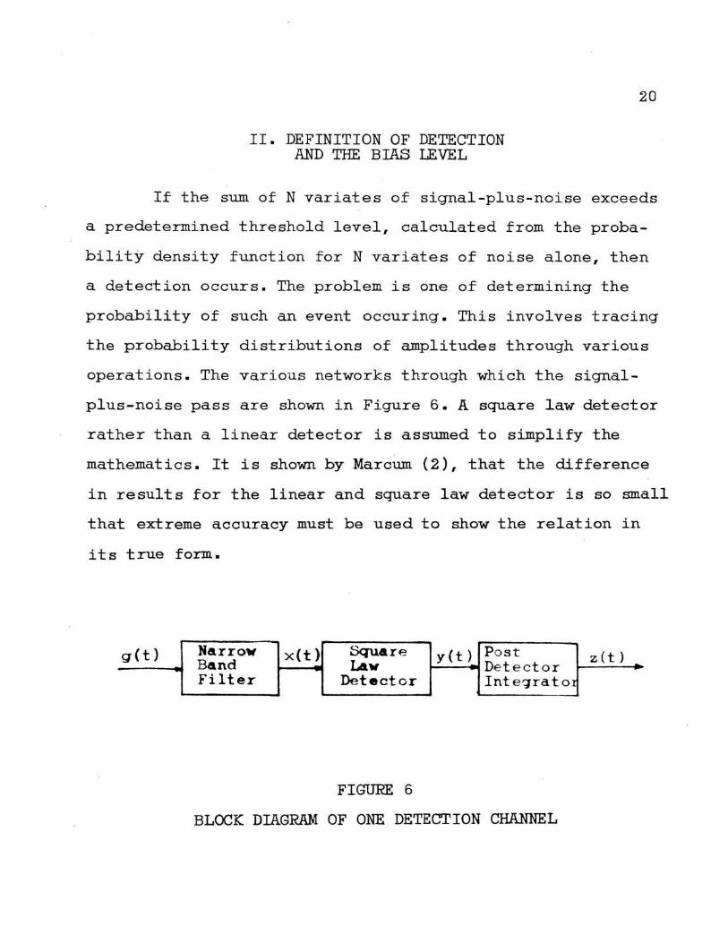
operations. The various networks through which the signal
plus-noise pass are shown in Figure 6. A square law detector
rather than a linear detector is assumed to simplify the
mathematics. It is shown by Marcum. (2), that the difference
in results for the linear and square law detector is so small
that extreme accuracy must be used to show the relation in
its true form.
g(t) Narrow x(t) Square y(t }_ Post z ( t ) - Band - I.Av Detector --- - -
Filter Detector Inteqrato1
FIGURE 6
BLOCK DIAGRAM OF ONE DETECTION CHANNEL

21
Threshold Level
The threshold level is determined by integrating the
probability density function of the noise voltage at the
output of the post detector integrator, for a partictular
false-alarm time or false-alarm probability. It is generally
assumed that the combination of shot, thermal, and cosmic
noise can be represented by the real gaussian distribution
p(g) = 1
J211'1g
2 2 exp { -g / 2 '1g) (11)
The probability density function of the noise envelope, V,
when passed through a linear narrow-band filter is given by,
Davenport (11)
2 2 2 p{V) = (V/rg) exp {-V /2rg) For V? 0 (12)
Since the detector input is a narrow-band gaussian random
process, then
x(t) = V cos (wet+ 8) {13)
The output of the square law device is
Passing y through an ideal low pass filter, a·filter which
will pass without distortion the low frequency part of its
input and filter out completely the high frequency part,
the output of the post detector integrator is
2 z = av / 2 (15)
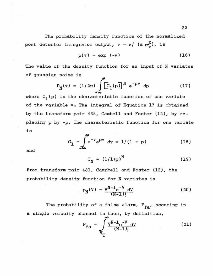
22
The probability density function of the normalized
post detector integrator output, v = z/ (a o-:2 ), is x
p(v) = exp (-v) (16)
The value of the density function for an input of N variates
of gaussian noise is 00
PN(v) = (1/2rr) J @1
(pl) N e -pv dp (17) -oo
where c1 {p) is the characteristic function of one variate
of the variable v. The integral of Equation 17 is obtained
by the transform pair 438, Cambell and Foster (12), by re-
placing p by -p. The characteristic function for one variate
is (JO
cl= Je-vepv dv - 1/(1 + p) (18}
and -oo
(19)
From transform pair 431, Campbell and Foster (12), the
probability density function for N variates is
(V) = vN-le-V dV ~ (N-l)I .
(20)
The probability of a false alarm, P fa, .occuring in
a single velocity channel is then, by definition, 00
p = JvN-le-V dV (21) fa (N-1)1 v .
T

23
The probability of a false alarm in a single velocity channel
is related to the post detection integration time, Ti, and
the single velocity channel false-alarm time, Tfa' by the
expression, Bussgang (5),
- TI /Tf 1 a (22)
Equation 21 now becomes ao
(T./T ) =j-yN-le-V dV (23) 1 fa (N-I)!
VT
In terms of the Incomplete Gamm.a Function, Pearson (13), u{p+l)l/2
I{u,p) = Je -v;P dv (24) p !'
0
Equation 23 becomes
(25)
from which the bias level is determined. Curves of the thres-
hold as a function of N and Pfa' as calculated by the author
of this thesis, are given in Figure 7.
Single-Look Probability
Marcum (1) and Bussgang (5) treats the single-look
probability of detecting a target in which the amplitude of
the returned signal pulses are not fluctuating. Swerling {3)
extends some of Marcums results to account for several kinds
of target fluctuationsa The type of targets considered in
24
this study are jet aircraft, missiles, and similar targets
in which the returned power is assumed constant for the time
on target during a single scan. However, the returned signal
fluctuates independently from scan-to-scan. This is Swerling's
Case,!.
Signal-plus-noise. The input signal-to-noise power
ratio has the probability density function, Swerling (3)
p(X,X) = (1/X) exp (-X/X) For X >O (26)
The probability, Ps, that N variates of signal-plus-noise
exceeds a given threshold on one look (scan) is, for N equal
to one
(27a)
For N greater than one, the expression for the probability is
P8
- 1 - I[!T/(N-1)112, N-~ + (1+1/NX)N-l •
• I~T/(N-1)1 / 2 (NX+N-l)(Nl'.)-l, N-~ exp (-VT/1-tfa)
(27b)
As shown by Swerling (3), for the cases of N~l and
the false-alarm time per channel is large, then the gamma
functions are very nearly unity and Equation 27b is approx
imated as
(28a)
25
or
This is the expression for the probability that a target of
given cross sectional area is detected by range Rx during
one look, one scan of the antenna. The curves and data pre
sented in the remainder of this thesis were computed by the
author. Curves of the single-look probability of detection
are shown in Figures 8, 9, and 10 for false-alarm probabilities
1 -5 -6 -7 of O , 10 , and 10 respectively. These curves do not
account for the possible effects of obscuring of the returned
signal.
Signal Obscuring. The high pulse repetition frequency
of a pulsed doppler radar leaves a very small receiving time
between transmitted pulses. For distant targets, it is quite
probable that the returned signal or a portion of the return
ed signal arrives while the receiver is gated off -. The result
is a decrease in the single-look detection probability.
Figure 11 illustrates the obscuring of the returned pulse
and its effect on the single-look detection curve.
The transmitted pulses of energy are r~presented in
Figure lla. The effect on the normalized range of the signal
returning at various instants of time is shown in Figure llb.
Figure llc shows the single-look probability of detection in
terms of normalized range for various values of signal obscuring.
Cf)
~ 0 > . U) . ::i:
•
20
15
10 9
8
7
6
5
4
c
a
n
a ()
0
o.---_____.
. .
o..--- -----o~ -
OL----'"
~ ~
~
~
~
-~ -
v . .
..
. .
x-sc - ~
--------------If!!' ____......
~
~ --H•3C ____.
--------- ~ ~
~ N-20 ~ --
~ ~
~ M•lC
/ /
/ ~
•,
~ .,,,,,,.
' N•l ··. : /
26
~,,, ~~ _,, ,.
,,/ .,,,,,. ,,,,,,, - ,,. ,,,_. .,,,, .,,~ ~,,. ~' ,,, .,,,,,, ,_, ,,,, . .,,,,,,,
__..,-"' •. / ~~
~· ,,,~ /~
~/
~' . ./ ,,,
/ ~,
v
~ v /
/ /
. -
10 1 1.s 2 2 .s 3 4 s 6 7 8 9 10
LI\ (~fa>
FIQURE 7
THRESHOLD LEVEL AS A FUNCTION OF THE NUMBER OF VARIATES INTEGRATED AND THE FALSE-ALARM
PROBABILITY

27
99-------------------------...... ---....--...---.~-r--..--. P • 10·
981r--1--~-+---+~--.-------~~------.----+-~....-----t~-...--..---.
pfa - Ti/ZTFA go~.....-~~-...--....-_.,--...-----4
TFA ~ FALSE-ALARM TIME
8 0 r--+---1iit--11r-1-_,...,.._--+_...,.______. Ti .. P • D • I • TIME
~ I • IIUIIBER OF VARIATES ~ 10~....---+--. .............. ~~..._........ IRTEGRATED
60i--'"\'t---+---+-....._ ..... .......,.....,_+-~ Bf
50t---t-r1~-+---+--........ ~~__...,. ...... ~ z
40r--~~t--~--~_.....~,.._ .......
• DOPPLER FILTER BAKDWIDTH
- IIUMBER ·oF DOPPLER FILTERS
UARE LAW DETEC OR 30~-r-~~-+---+---4~__....___._ .............. ...-.-.--=-......----.-------.------------4
2~--+-~+-__. __ ........ ~t---_... __ ........ ~~ ...... ---....... _..~-...---...-......
11---+---+-__. __ ....... __ "'-....... --........ ~t---_..,...,_....,._.......,.__.._...__...._ ......
o.s~_._~...,___. __ ....... _____ ~--...... --t---_...____..,._--4~-.-........ ....,_ .....
0.21----+-~+-~----_,._--1---+~ ...... -----_...--...... ~---....---~--1 0.1~-----~ ....... --~ __ .__,.... __ ...._~ ............... --........... ---~--J~r-ll
.4 .6 • R/R • ACTUAL RANGE
o NORMALIZING RANGE
Flg(JJl£ 8
SINGLE-LOOK PROBABILITY OF DETECTION IN TERMS OF NORMALIZED RANGE

99----~--~--------------------~------------------98.,._-+-~-+-~-+-__.~-.-~---------+-~-+-~-t-----.~---+-~-.---1
P = 10- 6 fa
: pfa = Ti/ZTFA go..--~.-......_~..---+---+---....-~
TFA - FALSE Al.AR)( TIME
8 O t----+---....--+1.---...~--+---+---+--~ T . - P • D • I • T IKE 1
- NUMBER OF VARIATES INTEGRATED
501---++-~-+-~~--+------.......-..--+-___..
40..--~----+-~-+-_..._. __ ...._...~ ...... ___,. Z
- DOPPLER FILTER BANDWIDTH
DOPPLER
30~---'--+-4-~+--+-',..--+-~~~~~"6MMll-...... .,.._~llt..a&J~~--___,
0. 5 .
0.2t----+--....,_--+-_..., __ ...... ~-+-----4~-+----+---.+--+~--+-...... -+--......
O.l'--_...~...._~...____... __ _.__...___....._ .......... __ .-_~ ......... -----------•4 .6 .8 1.0 1.2 1.4 1.6 1.8
ACTUAL RANGE R/Ro - NORMALIZING RANGE
FIGURE 9
SINGLE-LOOK PROBABILITY OF DETECTION IN TERMS OF NORMALIZED RANGE
99
98
95
· 90
80
70
60
50
40
30
20
10
5
2
1
o.s
0.2
0.1
~ ~ \
\
\ \
.4
29
Pc -10•"/ •• .
~ · pfa - Ti/ZTFA .
~ ~ TFA • FALSE-ALAR)I TIME
\ Ti • P.D.I. TDIE
\ ·'\' ~ I • IUJIBER OF VARIATES IJITEGRATED
~' '~ " Bf - DOPPLER FILTER \ ~\ ~~ BAHDWIDTH
~ .
. '\ ~'\ ,'\ z - KUIIBER OF DOPPLER FILTERS
\ ' ' ~'\ ~ ' Ai n&w IAll u•. 1".l~l]}i
\ \ \ l\.' I\. \ \ \ ~ \ " \ \ ;~ ~ " v:· •l \ 18 ~ ~ ~o '\ .·
\ \ ,-~ ~~ " .\ · \ \ \ ~ '\ ~
\ \
" ~ "' ~ .
i\ \ ' ~ ~
' \. • 6 •• 1 • J 1.2 1.4 1.6 l.
R/i • ACTUALRANGE o NORMALIZING RANGE
FI<aJII 10
SINGLE-LOOK PROBABILITY OF DETECTION IN TERMS OF NORMALIZED RANGE
8
30
The true single-look detection curve, shown in Figure
lld, is constructed by repeated application of Figures llb
and llc. The ratio of the signal and transmitter duty cycles
and thus the true detection curve depend on the rate of
closure between the radar and target and the position at
which the target enters the field of view of the radar. It
is quite laborious to construct the true detection curve each
time a different closing velocity is desired or a radar param
eter is changed.
It is equally probable that the returned signal will
arrive at any time in the period T if the exact position of
the radar and target is unknown. ·An average single-look de-
tection curve is calculated to account for the obscuring
effect by dividing the period into twenty equal divisions.
A detection curve is constructed for each division. If the
recovery time of the TR tube is assumed negligible, the ratio
of the signal to transmitter duty cycle is symmetrical about
T/2. Only the average of ten curves are then necessary to
construct the average curve. Figure 12 illustrates the aver
aging of the single-look detection curve for N = 1, Pfa = 10-5 ,
and a transmitter duty cycle of 0.25. The enclosed number by
the solid curve indicates that its value is weighted by the
factor 5.
The ratio of the normalized range between the unobscur
ed detection curve and the average detection curve is constant

·31
~49',.. . ~n nL..-_n..___ ____ n_. _ T ~T~ Time
(a) Transmitted Pulses ·
R · a_ fd;r. _y&----- -......iy......___y _____ j ~ ~at.~
Time .
(b) Obscuring Ratio
+' ~
100 Cl> CJ
M 80 a>
60 Cl.
~ 40 · H
Ill 20 Cl.
0 0 .1 • 2 .3 .4 .s • 6 . .7 .. • a
.fJ c: Q)
0
M
d! c:
H
0 • Cl.
100 ·ao 60 to 20
0
.. Normalized R•IM1•
(c) Sinqle-look Propability
.1
'\ j~ ~ , I "I
\ I \ ~~ ....
\. I ' ~ ·
\/ '\ .. ~ ~ii .3 • 4 .. s . .6
lorlllllized Ra11qe . ·
(d) True Detection CurYe
· FIGURE 11
TRUE DETECTION CURVE AND OBSCURING EFFECTS
-.~...._
.1 • 8

32
for constant values of (1) the single-look probability, (2)
the false-alarm probability, and (3) the transmitter duty
cycle. It is necessary to determine this correction ratio,
R, for one value of N for each given false-alarm probability c
and transmitter duty cycle. The average single-look detection
curve is obtained for a different value of N by multiplying
the unobscured detection range, for each given value of prob-
ability, by the corresponding value of the correction ratio.
The correction ratio was computed as illustrated in the pre-
vious paragraph for transmitter duty cycles of 0.25, 0.5, -5 -6 -7 and false-alarm probabilities of 10 , 10 , and 10 • The
results are presented in Table I.
Summary
Chapter III treated the single-look detection range.
A normalizing range was developed to relate the signal-to
noise power ratio. Equations for the threshold level and un
obscured single-look detection probability were given in
terms of false-alarm time, post detection integration time,
and the number of variates integrated.
A part of the returned signal energy is generally not
available for detection because of the high pulse repetition
frequency. A method was given to approximate the signal ob
scuring effect on the detection probability. Average single
look detection curves are computed by the use of Figure's
8, 9, and 10 and Table I.

N --....-4 w
Ul t:l.
I
~ Pal C..>
~
~ ~ H
z 0 H
t3 ~ E-4 ~ A
~ 0
~ H ~ H
I Cl..
33
Pfa-10-~d-0.25 9u-----~....__......,_...._ __ +-_____________________ .....
·a
7
6 \ \
5
4
3
') L,
10
5
2
1
o.s
0.2 0.1
0 •. 2 .4 R/R •
0
.6
pfa =- Ti/ZTFA
T • FAIBE-AIARJ( FA TIME
Ti • P. D. I. TIME
N =- NUMBER OF VAR.IATES INTEG.
B f • DOPPLER FILTER BAJIDWIDTH
Z =- NUMBER OF DOPPLER FILTER
\ ~
SQUARE IAW DETECTOR
.8 1.0. 1.2 ACTUAL RANGE
NORMALIZING RANGE
FIGURE 12
AVERAGE SINGLE-LOOK PROBABILITY OF DETECTION AT RANGE R IN TERMS
OF NORMALIZED RANGE

34
TABLE I
OBSCURED RANGE CORRECTION FOR SINGLE-LOOK DETECTION RANGE
Per Cent Transmitter Duty Cycle Transmitter Duty Cycle Single- of 0.25 of 0.5 Look Detection False-Alarm Probability False-Alarm Probability Range
10- 5 10- 6 10-7 10-5 10-6 10-7
95.0 0.5215 0.5514 0.5485 0.4154 a. 37 65 0.3418
90.0 0.5759 0.6003 0.6000 0.4528 0.4286 0.4158
85.0 0.6320 0.6354 0.6425 0.4990 0.4660 0.4630
80.0 0.6722 0.6727 0.6831 0.5172 0.5014 0.5044
7 5 .o 0.7127 0.7161 ·0.7156 0.5448 0.5313 0.5374
70.0 0.7462 0.7481 0.7429 0.5726 0.5605 0.5617
65.0 0. 7697 0.7783 0.7712 Oa5921 0.5854 0.5879
60.0 0.7886 0.7942 0.7864 0.6127 0.6052 0.6068
55.0 0.8089 0.8130 0.8090 0.6326 0.6288 0.6294
so.a 0.8276 0.8316 0.8252 0.6521 0.6445 0. 6471
45.0 0.8413 0.8494 0.8428 0.6692 0.6657 0.6650
40.0 0.8553 0.8552 0.8518 0.6839 0.6824 0.6790
35.0 0 .8670 0.8680 0 .8677 0~6982 0.6989 0.6984
30.0 0.8812 0.8787 0.8808 0.7077 0.7188 0.7136
25.0 0.8947 0.8912 0.8901 0.7342 0.7340 0.7270
20.0 0.9024 0.9023 0.9022 0.7496 0.7521 0.7460
15.0 0.9137 0.9157 0.9132 0.7667 0.7708 0.7653
10.0 0.9231 0.9281 0.9249 0.7842 0.7904 0.7879
35
TABLE I (continued)
Per Cent Transmitter Duty Cycle Transmitter Duty Cycle Single- of 0.25 of 0.5 Look Detection False-Alarm Probability False-Alarm Probability Range
10-5 10- 6 10-7 10-5 10- 6 10-7
5.0 0.9412 0.9393 0.9371 0.8089 0.8152 0.8136
2.0 0.9451 0.9489 0.9509 0.8305 0.8333 0.8380
1.0 0.9468 0.9416 0.9548 0. 8383 0.8439 0.8492
0.5 0.9585 0.9515 0.9558 0.8385 0.8489 0.8602
0.1 0.9548 0.9590 0.9570 0.8534 0.8643 0.8711

36
CHAPTER TV
CUMUIATIVE DETECTION RANGE
It is of interest to estimate the probability that the
target is detected by the time it has reached a specific
range, R. It is the purpose of this chapter to use the singlex
look: detection curves (average) of Chapter III to predict the
cumulative detection range for several flight geometries. An
approximate solution of the cumulative equation and the limit
of the radar aspect angle is considered.
I . CUMUIATIVE PROBABILITY
Assume a target enters the radars field of view at a
range R1/R0
• The cumulative probability that the target is
detected at least once by the time it reaches a range R /R X O
is
Rx/Ro Pc= 1 - rr,' ~ - Pso(R/RoJ
Rl/Ro
(29)
The range progresses from R1 /R0
to Rx/R0
in units of !::,.R/R0
•
The length of the normalized increments is determined by
where
(30)
TF - time required for the radar to complete one fra.xne.

Approximate Solution
Equation 29 is rewritten as
R /R Pc= 1 - exp ~ Ln [! - P
80(R/R
0})
R1/Ro
37
(31)
If the increments l:lR/R are sufficiently small to allow nego
ligible change in the P value, then the summation is approxso imated by an integral. Equation 31 becomes
.J, Rx/Ro } Pc= 1 - exp l(R
0/VRTF) S Ln Q- - P
80(R/RJ d(R/R
0) (32)
R1/Ro
Numerical integration must be performed, when applying
Equation 32, using the data supplied by Figures 8 through
10 and Table I. Figure 13 shows the value of the integral of
Equation 32 for a transmitter duty cycle of 0.5, N = 10, and
a false-alarm probability of 10-7 • The use of this curve is
illustrated by an example problem later in the chapter.
II. A PROCEDURE FOR DETECTION ·RANGE COMPUTATION
The procedure for computing the cumulative probability
of detection depends on the geometry associated with the
interceptor, target, direction of radar propagation, and the
range at which the target enters the radars field of view.
Several cases of flight geometry are considered in the follow
ing paragraphs. The procedures are given in step form for

-0 p.:; --p.:; -1J
s:a.. 0
-.
-10-
c .. '" " l"
2
3
4
,38
-lP -fa ilO-'
" 11-10
K daii:Q • ~
~
\..
' ' " ' \. "" "\
I\ ' - ..
'\.
\. \.' \
' ~ \
\ •'
.4 -.6 .8 R/R
0 • ACTUALRANGE
. NORMALIZING RANGE
FIQUII 13
VALUE OF INTEGRAL OF EQUATION 34 IN TERMS OF NORMALIZED RANGE
\
\ · \ \ ·\ \ _\
' \ ' \
1.0 1.2

ease of following the computations and in programming the
solution for a digital computer.
39
The first general step is to test the given angles,
which are defined in the following paragraph, to determine
the procedure to follow. The first step is:
(a) if a f nor 2rr: compute following the procedure of Case I.
(b) if a = n and n = e = 2rr ; compute PX X
following the procedure of Case II.
(c) if a= 2n, ~x f n, and ex~ 2rr; compute following the procedure of Case III.
Definition Of Symbols Used
The subscript x when used with a symbol indicates an
initial or given condition. The symbols used in the following
procedures are defined as:
e - angle enclosed by the interceptor line n of flight and the direction of radar propagation on the nth scan. (e is the . m maximum antenna look angle)
~ - radar aspect angle on the nth scan. n
a - angle enclosed by the interceptor and target lines of flight.
w - antenna angular rate of rotation.
& - radar beamwidth at the half-power points.
R - slant range between interceptor and n target on the nth scan.

~ - slant range at which it is assumed the target enters the radars field of view.
~n - targets range on the nth scan.
Rin - interceptors range on the nth scan.
D - hortizontal range between target and n interceptor on the nth scan.
C - perpendicular range between target and interceptor.
Ad - antenna diameter.
v1 - interceptor velocity.
VT - target velocity.
40
Case I. The geometry for two examples of flight con
ditions is shown in Figure 14. The doppler shift of the
target represented in Figure 14a always occurs in the non
clutter region if cos f3n(n/2. A. procedure for computing
the cumulative probability of detection by slant range R is x
outlined by the following steps.
1.
2.
3.
4.
~x t x
= R (sin 8 )/sin a. x . x
= ~x/VT •
= (Rxsin f3x)/sin a.
- -VIRa+VT~x+(VTRix-VI~x)cos a 2 2
VT+ VI - 2VTVI cos a
2 2 2 -(RI +R~ +2R- RI cos a - R) x --'l'x -... l'x x m

5.
6.
7.
8.
9.
10.
11.
Iater<Ntptor ____..
. (a)
l__TarCJet (b)
FIGURE 14
FLIGHT GEOMETRY FOR CASE I
Rrro = R.rx - VTto • e = arc sin (RT -R- )sin a/R • o · x --'l'o -m.
Check 1e0
f against teml • If 1e0 I> Jeml stop, no detection is possible.
t30
= 11 - (80
+ a) •
Obtain the value for o- (13 0 ) •
Compute R from Equation 8. 0
41

12 • N = ( oB f ) I w •
13. Pfa = Ti/Tfa •
14. Compute ~/R0
and read the value of Pso(o) from the curve corresponding to the values obtained in steps 12 and 13 and the transmitter duty cycle.
15. ~n = VT (t 0 + nTF) •
16. Rin = VI (t 0 - nTF) •
17. Rn = (~ + R~n - 2~nRin cos a)1
/2
•
18. en = arc sin (~n sina)/Rn.
19.
20.
Check fenl against Jeml as in step 7.
Q = 11· - ( 8 + a ) • ..,n . n
21. Obtain the value of O""'(f3 ) • . n
22. Compute R0
from Equation 8.
42
23. Compute Rn/R0
and read the curve of Pso as in
step 14 to obtain P ( ) • son
24. Repeat steps 15 through 23 letting n = 1, 2, 3, ••• until R = R • n x
25. Compute Pc from Equation 29.
The doppler ·frequency associated with the target in
Figure 14b always occurs in the clutter region if the target
velocity is less than or equal to the interceptor velocity.
The method of this study can not be used to predict the de-
tection range. The equations developed are based on non-
correlated samples. This particular geometry is not consider
ed in this thesis.
43
Case II. The flight geometry for Case II is shown in
Figure 15. This is seen to be a head-on collision course
which always results in the target's doppler appearing in the
clutte-r free region.
Tarqet 1 t ~ , C'\a. n erceptor 7 • ~ 4
FIGURE 15
FLIGHT GEOMETRY FOR CASE II
A procedure for computing the cumulative probability
of detection by range R is outlined by the following steps. x
1.
2.
3.
4.
t 0
6
N
Pfa
=~/(VT+ VI).
- 27.55 ("A./ Ad).
- ( 6Bf) /w •
- Ti/Tfa •
5. Compute R0
from Equation 8.
6. Compute Rm/R0
and read the value of P so(o) from the curve corresponding to the values obtained in steps 3 and 4 and the transmitter duty cycle.
7 • Rn = (VT + VI ) ( t O
- nT F) •
8. Compute Rn/R0
and read the curve of P60
as in step 6 to obtain the value of P ( so n) •

9. Repeat steps 7 and 8 • Stop when Rn=
10. Compute Pc from Equation 29.
R • x
44
Case III. Figure 16a illustrates an anti-parallel
flight path. A procedure for computing the cumulative prob
ability of detection by range Rx is outlined by the following
steps.
1. C = Rx sinl3x.
2. Do - (R! - c2)1/2 •
3. t0
- D0
/(VT + VI).
4. 130
= 80
= arc sin (C/~).
5. Compare f B0 J with jeml • If f e ol>J emJ set P ( ) equal to zero and proceed to step 11. so O
6 • o - 27 • 5 5 (1'../ Ad) •
7 • N - ( &Bf ) / w •
8.
9.
10.
11.
12.
13.
14.
15.
16.
pfa = Ti/Tfa •
Compute R0
from Equation 8.
Compute R /R and read the value of P ( ) -"'ln O so O
from the curve corresponding to the values obtained in steps 7 and 8 and the transmitter duty cycle.
Dn = (VT + VI)(to nTF).
Rn - (D2 + c2)1/2 n •
'3n = e n = arc sin (C/R ) • n
Compare l8nl with I eml as in step 5.
Obtain the value for er ( 13n) •
Compute Ro from Equation 8.

45
R dx · Interceptor
Tar99t . (a)
\ _Interceptor
(i,)
FIGURE 16
FLIGHT GEOMETRY FOR CASE III
17. Compute Rn/R0
and obtain the value for Pso(n) as in step 10.
18. Repeat steps 11 through 17 for n = 1, 2, ••• Stop when R = R n x
19. Compute Pc from Equation 29.
The parallel flight geometry illustrated in Figure 16b
is quite similar to the geometry of Figure 14b. This partic-
ular configuration is not considered for the same reasons
given in Case I.
Example Problem
To illustrate the use of the curves and equations, an

46
example problem is givena The approximate solution for the
cumulative probability of detection is used to illustrate its
advantages under certain cond.itionsa
borne
which
Pulsed doppler radar parameters. Assume that an air-
pulsed doppler radar has the following parameters:
pt - 2000 watts w -
d - 0.5 T. -l
I\. - 3.2 cm. TFA -
Ad - 32 inches z -
Bf - 357 c.p.s. TF -
L - 31.6 a- -
Calculations. Figure 17 illustrates a
is a special consideration of Case
VI= Mach 1
VT = Ma. ch O. 9
f3 -= n/6
Target
Interceptor
FIGURE 17
FLIGIIT GEOMETRY FOR A COLLISON COURSE
I.
100 deg. I se.c a
0.03 sec.
500 sec.
600
3 sec.
10 sq. m.
collison course,
The number of

47
computations is reduced by the use of the approximate solu-
tion when a collision course exists. The radar aspect angle,
the antenna look angle, and the relative closing velocity
are invariant. The cumulative probability of detection is
computed from an assumed range~ of 1.1 R0
to zero rangea
The results are shown in Figure 18. The probability of de
tection is found from the following steps:
la Compute the antenna gain.
G = 35.25 (Ad/;....) 2 = 35.25 (32/3.2) 2 - 3525
2. Compute R from Equation 8. 0
R - 1.012 (2xl0 3 )(3525) 2 (3.2) 2 (0.5)(10) 0
(357)(31.6)(1 - 0.5) R = 115.6 nautical miles.
0
3. Compute the closing velocity.
VR = G-T cos 13 + VI J 1 - (VT/V1 )2sin2~ (0.159)
VR - c 9 ( .866) + J 1 - (. 9 ) 2 (. 5) 2 J ( 0 .159)
VR - 0.2548 nautical miles per second.
4. R0
/VRTF = (115.6)/(0.2548)(3) = 151.2
5. o = 27.55 (;..../Ad)= 27.55 (3.2/32) = 2.8 deg.
6 • N = c oB f > I w = c 2 • 8 }( 3 s 7 ) / 1 o o = 1 o
7. Pfa = Ti/(ZTFA) = (0.03)/(600)(500) = 10-7
8. Obtain the value of the integral of Equation 34 at R/R = lal from the figure corresponding to the vafues of steps 6 and 7. For this example the figure is Figure 13 and the value obtained is (-0.000216).
Summary
48
9. Compute the value of Pc at R/R0
equal to 1.1 by Equation 34.
Pc= 1 - exp -{151.2)(0.000216) = 0.03217
10. R = 1.1 R0
- {l.1){115.6) = 127.16 n. mi.
11. Repeat steps 8, 9, and 10 until the desired minimum range is reached.
The cumulative probability of detecting a target of a
given cross section at least once by the time it has reached
a range Rx was treated. Only targets having their associated
doppler frequencies in the non-clutter region are soluble by
the methods presented.
Procedures for computing the cumulative detection
ranges are listed for three general cases. An approximate
solution and an example of its use is given to illustrate
the reduction in the number of computations from the general
procedure when a collison course exists.

49
0 10(
~ . . ~ I • ~ 9( tj \ · ~
80 ff ~ H
:z; 7C 0
\
\ /
. I\
\ H
tJ &: ~ ~
.\ . ·. \ :
~ 50 .... . 0 .-.,./ · .. \ .
~ ,, . H ,_ . ~ H \
I 30 . \ '
~ 20
~ 10 !
0
\ \
. ·"'~· ·O . . 20. 40 60 80 100 120
RANGE
FIGURE 18
CUMUI.ATIVE PROBABILITY OF DETECTION

50
CHAPTER V
CONCLUSIONS
This study presents a practical, although an approxi
mate, solution for the detection range performance of pulsed
doppler radars. The equations presented are based on (1) in
dependent samples, (2) target scintillation, (3) the target
and the interceptor are in the same geometrical plane, and
(4) the target doppler occurs in the clutter free region.
The curves and procedures given are applicable to most
radars. The curves presented can be applied to the prediction
of detection range performance-of pulsed and continuous wave
radars with few or no modifications.
It is felt that the procedure presented in this thesis
is sufficiently accurate for a rapid solution of the detection
capabilities of a pulsed doppler radar. This solution then
allows a comparison to be made between different radars such
as pulse, continuou_s wave, or pulsed doppler radars.
It is neces·sary to develop the threshold level and
the single-look detection equations for correlated samples
before it is possible to predict the detection range against
targets whose dopplers occur in the clutter region.
Three dimensional flight analysis should be investi
gated to establish the limits of the procedures presented
51
in this study. Comparison of the theoretical detection
ranges with the experimental data, as it becomes available,
is necessary to establish the validity of the theoretical
procedure.

1.
2.
3.
4.
5.
6.
7.
8.
52
BIBLIOGRAPHY
J. I. Marcum, "A Statistical Theory Of Target Detection By Pulsed Radar-Mathm.etical Appendix," Research Memorandum 753, The Rand Corporation, Santa Monica,
J. I. Marcum, •A Statistical Theory Of Target Detection By Pulsed Radar,• Research Memorandum 754, The Rand Corporation, Santa Monica, California,-rg-47.
P. Swerling, "Probability Of Detection For Fluctuating Targets," Research .Memorandum 1217, The Rand Corporation, Santa Monica, California, 1954.
D. L. Drukey, "Radar Range Performance,• Technical Memorandum No. 277, Hughes Aircraft Corporation, Culver City-;-t!aTITornia, (April 1954).
Bussgang, Nesbeda, and Safran, "A Unified Analysis of Range Performance of CW, Pulse, and Pulse Doppler Radar," Proc. I. R. E. Vol. 47 (October 1959), 1753-1762. --- --- --
Edward Barlow, •Doppler Radar," Proc. I. R. E. Vol. 37 (April 1949), 340-355. -- -- --
Louis Ridenour, Radar S~stems_En~ineering. Vol. 1 of The Massachusetts Institute of echnology Radiation I:a:E'oratory Series Edited by LOuis Ridenour. 28 vols. New York and London: McGraw-Hill Book Company, 1947.
R. Hollis, "Fals.e Alarm Time in Pulse Radar," Proc. 1.:. !h "E. Vo.l. 42, (July 1954), 1189.
9.- W.W. Maguire,· •Application Of Pulsed Doppler To AirBorne Radar Systems," Proc. National Aeronautical Conference (1958), 291-295.
10.
11.
The Doptler Effect And Its Aptlication To Do~ler -,ra'viga ors. The Ryan Aeronau ical Company,ectronics
Division Kearny Mesa Plant, San Diego 12, California.
Davenport and Root, Random Signals and Noise. New York and London: McGraw-Hill Book Company, 1958.

12.
13.
Campbell and Foster, Fourier Integrals for Practical Applications. New York and London: D. Van Nostrand Company, 1948.
K. Pearson. Tables of the Incoafutete Gamma-Function. Cam.bridge University Press, C ridge, England, published by Biometrika, 1946.
53

54
VITA
The author was born October 6, 1931, at Phoenix,
Missouri. He attended elementary and high school at Monett,
Missouri.
In December 1948, he accepted employment as agent
telegrapher for the Eastern Division of the St. Louis-San
Francisco Railway Company. He entered the United States Air
Force in June 1949. He attended the ground radar technicians
school at Kessler Air Force Base, Mississippi. Upon completion
of the school, the remaining two and one-half years were spent
as a radar supervisor and technician at McCord Air Force Base,
Washington. In December 1952, he was honorably discharged and
returned to the employment of the St. Louis-San Francisco
Railway Companya
In September 1953, he enrolled at the Missouri School
of Mines and Metallurgy at Rolla, Missouri. He completed the
requirements for . the Bachelor of Science Degree in Electrical
Engineering January 1957, at which time he enrolled in the
graduate school and became a member of the faculty as an
instructor in Electrical Engineering.
Industrial experience to this date includes summer
employment and consulting positions with the McDonnell Air
craft Corporation at St. Louis, Missouri.