A Method for Simulating Two-Phase Pipe Flowwith Real Equations of State

M. Hammer∗, A. Morin

SINTEF Energy Research, P.O. Box 4761 Sluppen, NO-7465 Trondheim, Norway

Abstract

Common two-fluid models for pipe flow assume local non-equilibrium regarding phasetransfer. To solve the two-fluid models together with accurate equations of state for realfluids will in most cases require mechanical, thermal and chemical equilibrium betweenthe phases. The reason is that reference equations of state for real substances typicallydescribe full thermodynamic equilibrium. In this paper, we present a method for nu-merically solving an equilibrium model analysed by Morin and Flåtten in the paper Atwo-fluid four-equation model with instantaneous thermodynamical equilibrium, 2013.

The four-equation two-fluid model with instantaneous thermodynamical equilib-rium is derived from a five-equation two-fluid model with instantaneous thermal equi-librium. The four-equation model has one mass equation common for both phases,but allows for separate phasic velocities. For comparison, the five-equation two-fluidmodel is numerically solved, using source terms to impose thermodynamical equilib-rium. These source terms are solved using a fractional-step method.

We employ the highly accurate Span-Wagner equation of state for CO2, and use thesimple and robust FORCE scheme with MUSCL slope limiting. We demonstrate thatsecond-order accuracy may be achieved for smooth solutions, whereas the first-orderversion of the scheme even allows for a robust transition to single-phase flow, also inthe presence of instantaneous phase equilibrium.

Keywords: two-fluid model, finite volume, FORCE scheme, Span-Wagner equationof state, isochoric–isoenergetic flash

1. Introduction

In the frame of CO2 capture and storage (CCS), large amounts of CO2 have tobe transported between the point of capture and the point of injection. In the two-degree scenario of the International Energy Agency [1], about seven gigatonnes ofCO2 emissions will be contained using CCS in 2050. This requires the development ofan extensive CO2 transport network. For large volumes of CO2, pipeline transport isan option.

There are challenges related to the operation of a CO2 pipeline, both in normaloperation and during depressurisation events, either planned or accidental. The safetyof operation has to be ensured, and it has to be demonstrated to the regulatory bodies.

∗Corresponding author. Tel.: +47 735 97 251Email addresses: morten.hammer [a] sintef.no (M. Hammer), alexandre.morin [a]

sintef.no (A. Morin)

Preprint submitted to Elsevier 28th April 2014

To facilitate this, and to reduce costly experimental procedures, reliable and accuratenumerical simulation tools have to be developed.

In pipelines, the CO2 will generally be transported in a dense phase, supercriticalor liquid. However, during transient events, gas or solid phases may appear. In addi-tion, impurities from the capture process will be present in the CO2. These impuritiesmay be for example water, residual chemicals or gases from combustion. They willimpact the thermodynamic behaviour of the CO2, for example the mixture density orthe temperature of the mixture during phase change.

It is common to use the stiffened-gas equations of state, when modelling two-phaseflow [2, 3, 4, 5]. It has a simple analytical form, and can be used to describe meta-stable fluids. For long pipelines transporting CO2 rich multi-component mixtures froma capture cite to an offshore injection well, these models might not predict the fluidproperties accurately. In this case it is important to use real equations of state. The realequations of state are generally only valid for full thermodynamical equilibrium.

At least two types of transient events have to be studied, with very different charac-teristics. The first type covers the fast depressurisation events that occur when the pipecontent is discharged to the atmosphere, either due to shutting down the pipeline, ordue to a fracture [6]. The second type covers the load variations in the pipeline in nor-mal operation, due to the capture processes delivering varying amounts of CO2. Theseload variations will have time scales in the order of several hours.

The kinetics of heat transfer between the phases, and of phase change can mostprobably not be neglected in fast transients related to fast depressurisation events. How-ever, during slow transients related to load variation, one is interested in predicting theresponse of the mixture in the pipeline, to avoid too low temperatures or phase changethrough pumps for example. During these slow transients, the most important is to havea very accurate equation of state to describe CO2-rich mixtures, rather than to describethe kinetics of internal heat transfer or phase change very accurately. The time scalesof these processes are negligible compared to the time scale of the relatively slow loadvariation. Very accurate equations of state can be obtained for mixtures at equilibrium.Thus it seems to be reasonable to use a full-equilibrium fluid-dynamical model in thiscase, to be able to benefit from the equilibrium equations of state.

Therefore, in the present work, we study full equilibrium fluid-dynamical modelswhere phase change and heat transfer between the phases are assumed to be instantan-eous. The framework supports any equation of state, thus impurities may be added byusing an equation of state for mixtures. Here we are using a very accurate equation ofstate for pure CO2 [7]. We compare two approaches. The first one is based on a fluid-dynamical model out of chemical equilibrium, the two-fluid five-equation model withphase change [8]. Instantaneous phase change is achieved by performing flash calcu-lations between each time step, such that the mixture returns to chemical equilibrium.The second one is based on a full-equilibrium two-fluid four-equation model presentedin [9].

Numerical results are presented to show the performance of the methods, and tocompare them to each other. The models have been solved using the finite-volumemethod with the FORCE flux [10, Sec. 14.5.1] and the second-order extension MUSCL[11]. They show that the four-equation based approach performs better in terms ofcomputational time than the five-equation based approach. It also shows that we canachieve second-order convergence rate in smooth regions, and that the method satis-factorily handles the transition to single-phase flow.

In Section 2, the five-equation model is presented, as well as the procedure to ensurechemical equilibrium between the phases. Then, the four-equation model is presented

2

in Section 3. In Section 4, the equation of state as well as the procedure to evaluate thenew state of the fluid are explained. The characteristic wave-structure of the modelsare presented in Section 5. Subsequently, the numerical methods employed to solve thetransport systems are described in Section 6. Finally, Section 7 shows the results of thenumerical test cases, and Section 8 summarise this work.

2. The five-equation model with phase change

The one-dimensional two-fluid models describe one-dimensional two-phase flowsin pipes. In the six-equation model, the phases are at mechanical equilibrium [8]. Thismeans that the two phases are at the same pressure at all times. The model is wellknown in the literature [12, 13, 4, 14, 15], and used in commercial simulation tools likeCATHARE [16] or RELAP5 [17].

The five-equation model [8] is derived from the six-equation model by assuminginstantaneous thermal equilibrium. This means that the phases are now at the samepressure and temperature at all times. This model contains one mass and one mo-mentum equation for each phase, while only one mixture energy equation is present.This model is similar to the model used by the commercial flow simulation tool OLGA[18]. When viscous terms are neglected, and all external forces but gravity are ignored,the system of equations for the one-dimensional five-equation model becomes

∂(ρgαg)∂t

+∂(ρgαgvg)

∂x= Ψ, (1)

∂(ρ`α`)∂t

+∂(ρ`α`v`)

∂x= −Ψ, (2)

∂(ρgαgvg)∂t

+∂(ρgαgv2

g)

∂x+ αg

∂p∂x

+ τi = viΨ + ρgαggx, (3)

∂(ρ`α`v`)∂t

+∂(ρ`α`v2

` )∂x

+ α`∂p∂x− τi = −viΨ + ρ`α`gx, (4)

∂(Eg + E`)∂t

+∂(Egvg + αgvg p)

∂x+∂(E`v` + α`v`p)

∂x= gxαgρgvg + gxα`ρ`v`, (5)

where the total energy Ek of phase k ∈ {g, `} is the sum of kinetic and internal energy,

Ek = ρkαk

(12

v2k + ek

). (6)

e is the specific internal energy.Further, ρ is the mass density, v is the velocity, p is the pressure, α is the volume

fraction, and gx is the gravitational component along the x-axis. Ψ is the mass-transferrate from the liquid to the gas phase, τi is the interfacial momentum exchange and vi isthe interfacial momentum velocity. The volume fractions must satisfy

αg + α` = 1. (7)

The interfacial momentum exchange is modelled with a differential term. In thisterm, the factor ∆p represents the difference between the average bulk pressure and thepressure at the gas-liquid interface. In this work we use

τi = −∆p∂α`∂x

. (8)

3

For practical simulations, ∆p should be physically modelled to account, for example,for the hydrostatic pressure in the liquid phase, or for the interfacial tension. However,for the purpose of the general model analysis performed in the present article, ∆p ishere chosen to be [19, 8]

∆p = δαgα`ρgρ`

α`ρg + αgρ`(vg − v`)2, (9)

where δ = 2.The unknowns of the system (1)–(5) are αg, α`, vg, v`, p, ρg, ρ`, eg and e`. However,

since we will be using the equation of state to solve the system, the temperature T mustbe included in the list. We have thus 10 unknowns. The 10 equations are (7), thetransport equations (1)–(5), plus two thermodynamic relations per phase given by theequation of state.

We may split the system (1)–(5) into two parts, which will prove useful in thecourse of the article. The first part is the flow model (1)–(5) where phase change isignored (Ψ = 0), while the second part only contains the contributions of phase change

∂(ρgαg)∂t

= Ψ, (10)

∂(ρ`α`)∂t

= −Ψ, (11)

∂(ρgαgvg)∂t

= viΨ, (12)

∂(ρ`α`v`)∂t

= −viΨ. (13)

The energy equation has disappeared in the second system, because mixture energy isnot concerned by phase change, it is only an internal transfer.

The speed of sound of this model is [8, 9]

cTF5 =

√√√√√√√√√√√ αgρ` + α`ρg

ρgρ`

αg

ρgc2g

+α`ρ`c2

`

+αgρgCp,gα`ρ`Cp,`T

(Γgρgc2

g−

Γ`

ρ`c2`

)2

αgρgCp,g+α`ρ`Cp,`

, (14)

where ck is the single-phase speed of sound of phase k, and Cp,k is its specific heatcapacity and Γk its first Grüneisen parameter, defined by

Γk =1ρk

∂p∂ek

∣∣∣∣∣ρk

=1

CV,kρk

∂p∂T

∣∣∣∣∣ρk

. (15)

Remark that the speed of sound is only a function of the differential terms. It is notaffected by the algebraic source terms modelling phase change.

2.1. Phase changeIn the five-equation model (1)–(5) described above, the phases are generally out

of chemical equilibrium. The mass transfer rate Ψ should then make the chemicalpotentials of the phases µk converge towards each other through phase change. A com-mon way is to set the mass-transfer proportional to the difference in chemical potential[20, 21, 22],

Ψ = K(µ` − µg

), K ≥ 0. (16)

4

If the potential of the liquid phase µ` is greater than that of the gas phase µg, masswill be transferred from the liquid phase to the gas phase and vice versa, at a rateproportional to K .

The phase change will also be accompanied by a transfer of momentum betweenthe phases, while the mixture momentum will be conserved. Writing the part of thesystem (10)–(13) – which performs phase change – in differential form, we obtain

d

∑k

(ραv)k

= 0, (17)

d(ραv)g = d(ρα)g vi, (18)

whered(ρα)g = Ψ dt. (19)

2.2. The interface velocity

Morin and Flåtten [9] showed that if the interfacial velocity vi is independent of thechemical potentials, the expression

vi =12

(vg + v`

), (20)

is the only one which ensures that mass change will never decrease the entropy of theflow. Remark also that the following differential relations can be written

dmg = − dm`, (21)

d(mv)g =12

(vg + v`

)dmg, (22)

d(mv)` =12

(vg + v`

)dm`, (23)

d(mv)g = d(mv)` (24)

where mk = (ρα)k is the phase mass per volume. Then, developing the total differentialfor the kinetic energy

d

12

(mv)2g

mg+

12

(mv)2`

m`

= vg d(mv)g −12

v2g dmg + v` d(mv)` −

12

v2` dm`, (25)

in which we substitute the relations (21), (22) and (23), we find that

d(

12

mgv2g +

12

m`v2`

)= 0. (26)

Thus, as noted by Stewart and Wendroff in [23], the kinetic energy of the mixture isnot affected by phase change. This means that the model (1)–(5) can first be solvedwithout phase change (system (1)–(5) with Ψ = 0), before the phase fractions areupdated through phase change in a separate step. If the kinetic energy had been affectedby the mass transfer, we would have had to solve simultaneously the thermodynamicequilibrium and the phasic velocities.

5

2.3. Instantaneous phase changeIf phase change may be assumed to be instantaneous (K → ∞ in (16)), an equilib-

rium equation of state (EOS) may be used. Such an EOS describes multiphase mixturesat equilibrium. For example, the Span-Wagner EOS [7] is very accurate for CO2 in gas,liquid and supercritical phases. One possible approach is to take advantage of the re-mark above. After the model (1)–(5) without phase change (Ψ = 0) has evolved for onetime step, the two phases will in general be out of chemical equilibrium. The secondpart of the time step is therefore to come back to equilibrium through phase change(system (10)–(13)). This approach is a fractional-step method [24, p. 380], also calleda time-splitting strategy [25, 4].

First, the phasic masses have to be determined so that the mixture is at equilib-rium. The mixture mass is given as the sum of phasic masses, (1) and (2), and theoverall energy is given from (5). Using the result from (26), the internal energy canbe calculated. The resulting problem is to solve a constant density and internal energy(isochoric–isoenergetic) flash. Since there is a momentum transfer between the phases,the new phasic velocities then have to be determined. We can write the equations ex-pressing the conservation of the mixture momentum and mixture kinetic energy as

(mv)n∗g + (mv)n∗

` = (mv)ng + (mv)n

` , (27)12

(mv2

)n∗

g+

12

(mv2

)n∗

`=

12

(mv2

)n

g+

12

(mv2

)n

`, (28)

where n∗ represents the state before applying phase change, and n is the state afterapplying phase change.

This gives a quadratic equation for the velocities. Its discriminant ∆ is written as

∆ = mn`m

ngmn∗

` mn∗g

(vn∗

g − vn∗`

)2, (29)

which is never negative, so that we will always have real roots. The roots of vn` are

vn` = vn

m ±

∣∣∣vn∗g − vn∗

`

∣∣∣ √mn`mn

gmn∗`

mn∗g

mn`

(mn∗

g + mn∗`

) (30)

where

vnm =

mn∗g vn∗

g + mn∗` vn∗

`

mn∗g + mn∗

`

(31)

may be defined as the mixture velocity. A criterion is now required to select the correctroot. Equations (21) and (23) give

dv` =dmg

2m`

(v` − vg

), (32)

while the differentiation of (30) with respect to mng evaluated for mn

` = mn∗` provides the

relation

dvn` = ±

dmng

2mn∗`

∣∣∣vn∗g − vn∗

`

∣∣∣ . (33)

Comparing equations (32) and (33), the correct root for vn` can be determined, and is

vn` = vn

m +

(vn∗` − vn∗

g

) √mn`mn

gmn∗`

mn∗g

mn`

(mn∗

g + mn∗`

) . (34)

6

Now, the gas velocity can be expressed as a function of the liquid velocity, and thegas velocity, vn

g, becomes

vng = vn

m −

(vn∗` − vn∗

g

) √mn`mn

gmn∗`

mn∗g

mng

(mn∗

g + mn∗`

) . (35)

Remark that in the case of a single-phase flow, we have vn` = vn

m and vng = vn

m.Note that the mass-transfer rate Ψ is never explicitly evaluated. The flash calcu-

lation implicitly transfers mass from one phase to the other so that the mixture is atequilibrium.

2.4. Integration procedure

To summarise, the integration of the system (1)–(5) from time step n − 1 to timestep n is split in four steps, introducing an intermediate time step, n∗.

1. Integrate the system (1)–(5) where phase change is ignored (Ψ = 0) from timestep n − 1 to n∗. The composite variables, (αρv)n∗

` , (αρv)n∗g , (αρ)n∗

` , (αρ)n∗g , and

En∗ = (Eg + E`)n∗ are then known.2. Calculate mixture density,

ρnm =

∑k∈{g,`}

(ρα)n∗k , (36)

and mixture internal energy,

(ρe)nm = En∗ −

12

∑k∈{g,`}

[(ραv)n∗

k

]2

(ρα)n∗k

, (37)

using composite variables from the intermediate time step n∗. Further, calculateT n, αn

gαn` , ρ

ng and ρn

` by solving a isochoric–isoenergetic flash given the mixturedensity and internal energy. This problem will be further described in Section 4.The pressure is then given by the thermodynamics, pn = p(T n, ρn

g) = p(T n, ρn` ).

3. Calculate new velocities vng and vn

` from equations (34) and (35).4. Update the composite variables for momentum and mass ((αρv)n

` , (αρv)ng, (αρ)n

`

and (αρ)ng).

2.5. Vector expression of the model

To summarise, with some rearrangement of the derivatives, and introducing theenthalpy, h = e + p/ρ, we can write the five-equation model in vector form as

∂u∂t

+∂ f (u)∂x

+ B (u)∂w (u)∂x

= s (u) , (38)

7

where

u =

αgρgα`ρ`αgρgvgα`ρ`v`

Eg + E`

, f (u) =

αgρgvgα`ρ`v`

αgρgv2g + αg∆p

α`ρ`v2` + α`∆p∑

kαkρkvk

(12 v2

k + hk

)

,

s(u) =

Ψ

−Ψ12

(vg + v`

)Ψ + ρgαggx

− 12

(vg + v`

)Ψ + ρ`α`gx

gx∑kαkρkvk

, B(u) =

00αgα`0

, (39)

w(u) =[p − ∆p

].

2.6. Algebraic source terms and wave propagation

In the fractional-step method described in Section 2.4 the flux part of the model,f (u) and w(u) in (39), is solved alternately with the algebraic part s(u). Now, thealgebraic source terms should affect the propagation of the waves predicted by theflux part of the model. This does not happen explicitly in the present method. Thewaves predicted by the flux-based solver are corrected a posteriori using the sourceterms. Particularly, instantaneous phase change slows down the intrinsic mixture speedof sound of the model. Thus, the speed of sound (14) over-estimates the actual speedof sound of the model with instantaneous phase change. Now, the speed of sound isused in the stability criterion of the scheme – the CFL number – thus the time steps areunnecessarily short. By including instantaneous phase change in the flux part of thesystem, we obtain a more faithful mixture speed of sound, thus the numerical methodscan use larger time steps. This reduces the simulation time.

3. The four-equation model

We now want to derive a four-equation model which is equivalent to the five-equation model (1)–(5) when the phase change is instantaneous. The transformationdescribed in the following is used to integrate the algebraic source terms in the fluxes,giving a full-equilibrium model.

3.1. Expression of the system

The full-equilibrium fluid-dynamical model is obtained by summing the two massequations (3) and (4), and adding the constraint that the phasic chemical potentialsshould be equal to each other at all times. This leads to the two-fluid four-equation

8

model with instantaneous phase change [9]

∂(ρgαg + ρ`α`)∂t

+∂(ρgαgvg + ρ`α`v`)

∂x= 0, (40)

∂(ρgαgvg)∂t

+∂(ρgαgv2

g)

∂x+ αg

∂p∂x

+ τi + viK(µg − µ`

)= ρgαggx, (41)

∂(ρ`α`v`)∂t

+∂(ρ`α`v2

` )∂x

+ α`∂p∂x− τi − viK

(µg − µ`

)= ρ`α`gx, (42)

∂(Eg + E`)∂t

+∂(Egvg + αgvg p)

∂x+∂(E`v` + α`v`p)

∂x= gxαgρgvg + gxα`ρ`v`. (43)

Now, since the phase change is instantaneous and µg = µ`, the term K(µg − µ`

)is

undefined. The analysis in [9] shows that it takes the form

K(µg − µ`

)= V(u)

∂(αgvg + α`v`

)∂x

+ P(u)∂p∂x

(44)

in the limit K → ∞, where it is assumed that

vi =

(vg + v`

)2

. (45)

The expressionsV(u) and P(u) are given by

V(u) =ρgρ`

α`ρg + αgρ`

TL

(αgρgCp,gχg + α`ρ`Cp,`χ`

)c2

TF4, (46)

and

P(u) =αgα`ρgρ`(vg − v`)α`ρg + αgρ`

TL

(ρ`Cp,`χ`

ψg

ρgc2g− ρgCp,gχg

ψ`

ρ`c2`

)c2

TF4, (47)

where the speed of sound of the four-equation two-fluid model is

cTF4 =

√√√ α`ρg + αgρ`

ρgρ`

(αg

ρgc2g

+α`ρ`c2

`

+ T(αgρgCp,gχ

2g + α`ρ`Cp,`χ

2`

)) , (48)

and the following shorthands have been used

χg =Γg

ρgc2g

+ρg − ρ`

ρgρ`L, (49)

χ` =Γ`

ρ`c2`

+ρg − ρ`

ρgρ`L, (50)

ψk = 1 + ρkTCp,kΓkχk, (51)L = hg − h`. (52)

The momentum exchange between the phases τi remains the same as in the five-equation model, and is modelled as in (8).

9

3.2. Vector form of the model

To summarise, the four-equation model can be written in vector form

∂u∂t

+∂ f (u)∂x

+ B (u)∂w (u)∂x

= s (u) , (53)

where

u =

αgρg + α`ρ`αgρgvgα`ρ`v`

Eg + E`

, f (u) =

αgρgvg + α`ρ`v`αgρgv2

g + αg∆pα`ρ`v2

` + α`∆p∑kαkρkvk

(12 v2

k + hk

) ,

s(u) =

0

ρgαggx

ρ`α`gx

gx∑kαkρkvk

, B(u) =

0 0 0

viV αg + viP −αg−viV α` − viP −α`

0 0 0

, (54)

w(u) =

αgvg + α`v`p

∆p

.4. Algorithm to evaluate the primitive variables

When the model have been advanced one time step, only the new composite vari-able vector u is known. However, to evaluate the fluxes ( f (u), w(u)) and the coefficientsof B(u) in (39) and (54), the primitive variables (pressure, temperature, gas volumefraction, phasic velocities, phasic internal energies) have to be known. In the presentsection, we will first present the EOS used to evaluate the thermodynamical state of themixture. Then we will explain how the primitive variables are calculated.

4.1. The Span-Wagner reference equation of state for CO2

The Span-Wagner reference EOS comprises an expression for the CO2 Helmholtzfree energy a(T, ρ) [7]. The reduced non-dimensional Helmholtz free energy equation

Φ(τ, δ) =a(τ, δ)

RT= Φ0(τ, δ) + Φr(τ, δ), (55)

is composed of an ideal contribution, Φ0, and a residual contribution, Φr. R is theuniversal gas constant. The reduced Helmholtz functions are expressed in terms ofthe reduced density, δ = ρ/ρcrit, and inverse reduced temperature, τ = Tcrit/T , whereρcrit and Tcrit are the critical density and the critical temperature, respectively. Theexpression for the reduced ideal part is

Φ0(τ, δ) = ln(δ) + a01 + a0

2τ + a03 ln(τ) (56)

+

8∑i=4

a0i ln

[1 − exp

(−τθ0

i

)].

10

0.01

0.1

1

10

100

1000

180 200 220 240 260 280 300 320 340

p(M

Pa)

T (K)

Solid

Liquid

Vapour

Figure 1: Phase diagram for CO2.

The expression for the reduced residual part is

Φr(τ, δ) =

7∑i=1

niδdiτti (57)

+

34∑i=8

niδdiτti exp (−δci )

+

39∑i=35

niδdiτti exp

(−αi (δ − εi)2 − βi (τ − γi)2

)+

42∑i=40

ni∆biδ exp

(−Ci (δ − 1)2 − Di (τ − 1)2

),

where ∆ = {(1−τ)+Ai[(δ−1)2]1/(2Bi)}2+Bi[(δ−1)2]ai . In this work the same coefficientsa0

i , θ0i , ni, ai, bi, ci, di, ti, αi, βi, εi, γi, Ai, Bi,Ci and Di as published in [7], are used.

By differentiation of the Helmholtz function, all required thermodynamic proper-ties can be derived. The differentials for the CO2 Helmholtz function are found in theoriginal paper by Span and Wagner [7]. As seen from equations (56)–(57), the Span-Wagner EOS contains many terms, including logarithms and exponentials, making itcomputationally demanding.

The Span-Wagner EOS is valid from the triple-point temperature to 1100 K andfor pressures up to 800 MPa. Span and Wagner also provided auxiliary equations forthe sublimation line and the fusion line. These equations are used together with thesaturation line calculated from the Helmholtz function for pure CO2 to plot the phasediagram in Figure 1. The dotted line continuing the saturation line above the criticalpressure and temperature represents (∂2P/∂ρ2)T = 0. The triple and critical point ofCO2 are displayed in Table 1. Pressures/temperatures for the test cases are selected atthe saturation line in the range between the triple and critical point.

4.2. Five-equation model

To calculate the primitive variables for the five-equation model, the procedure fromSection 2.4 is applied. The most challenging and CPU intensive part of the procedure

11

Table 1: Critical and triple point of CO2. Data taken from [7].

Property Symbol Value

Critical temperature Tcrit 304.1282 KCritical pressure Pcrit 7.3773 MPa

Triple point temperature Ttr 216.592 KTriple point pressure Ptr 0.51795 MPa

is step 2, where intensive properties, T and P as well as the phase fractions must be cal-culated. Thermodynamically, the equilibrium condition of this isochoric–isoenergetic(ρe) problem represents a global maximum in the entropy of the system [26]. The nu-merical algorithm used to solve the ρe problem are based on the method of Giljarhuset al. [27], and discussed in more detail in Hammer et al. [28].

In this work only single-phase, liquid or gas, and liquid-gas equilibrium are con-sidered. The single-phase equation is simply

e(T, ρspec) − espec = 0, (58)

where ρspec and espec are the specified density and specific internal energy. Equation(58) must be solved for the unknown temperature, T . It should be noted that solvingEquation 58 can produce a meta-stable solution. In case of a meta-stable solution, thereexists a liquid-gas solution with higher entropy. The single-phase solution must there-fore be tested for stability. If introduction of a new phase give an increase in entropy,the single phase solution is discarded, and a liquid-gas solution is sought instead.

To solve the ρe problem for liquid in equilibrium with gas, both the equilibriumconditions, Pg = P` and µg = µ`, and the density and internal energy specificationequations must be fulfilled:

P(T, ρg) − P(T, ρ`) = 0, (59)µ(T, ρg) − µ(T, ρ`) = 0, (60)

zge(T, ρg) + (1 − zg)e(T, ρ`) − espec = 0, (61)zg

ρg+

(1 − zg)ρ`

−1

ρspec= 0. (62)

Here zg denotes the gas mass fraction. The unknowns of the liquid–gas equation system(59)–(62) are [ρg, ρ`,T, zg].

Both (58) and the equation system (59)–(62) are solved using a second-order New-ton method.

4.3. Four-equation model

The challenge for the four-equation model is that the distribution of the overallenergy in kinetic and internal energy is not known a priori. It has to be evaluatedthrough iterations. The proposed procedure to evaluate the primitive variables usesa successive substitution approach. Using j as iteration index, the procedure is asfollows:

1. Assume, mn+1, j=0g = mn

g and mn+1, j=0`

= mn` , and calculate the phasic velocities,

vn+1, j=0g and vn+1, j=0

`, from the composite momentum variables.

12

2. Calculate T n+1, j, pn+1, j, αn+1, jg and ρn+1, j

g etc. using composite variables for massand energy. The same problem as described in Section 4.2 must be solved.

3. Calculate new velocities, vn+1, j+1g and vn+1, j+1

`, from the new phase masses, mn+1, j+1

g

and mn+1, j+1`

.

4. If∣∣∣∣mn+1, j+1

g − mn+1, jg

∣∣∣∣ < ε exit loop. Otherwise increment j and repeat from step

2. ε = 10−11 have been used in all simulations.

5. Characteristic wave-structure of the models

The characteristic wave structure of the two-fluid models is not known in general.In the case of equal phasic velocities, two of the eigenvalues correspond to acousticwaves, while the remaining ones are equal to the mixture velocity. These waves areentropy and volume-fraction waves (cf. [29] for the six-equation model, [8] for thefive-equation model and [9] for the four-equation model).

When relaxation source terms are added, the characteristic wave structure is nolonger clearly defined [30]. However, when the relaxation becomes instantaneous, thecharacteristic wave structure converges to that of the relaxed system. Thus, by per-forming the instantaneous chemical relaxation of the five-equation model numerically,we expect to recover the structure of the four-equation model.

6. Numerical methods

The fluid-dynamical models are solved using the finite-volume method with theFORCE flux [10, Sec. 14.5.1]. The integration formula is

un+1i − un

i

∆t+

f FO,ni+1/2 − f FO,n

i−1/2

∆x= 0, (63)

where uni is the variable vector at time step n and in cell i. f FO,n

i+1/2 is the FORCE flux attime step n and at the interface i + 1/2. ∆t and ∆x are the time and spatial steps.

The FORCE flux [10, Sec. 14.5.1] combines two components. The first one is thevery robust Lax-Friedrichs flux

f LFi−1/2 =

12

( f (ui−1) + f (ui) − a (ui − ui−1)) , (64)

where the cell flux f (u) is given in Sections 2.5 and 3.2. a = ∆x/∆t, and a (ui − ui−1)plays the role of extra numerical viscosity. The second component in the FORCE flux isthe Richtmyer flux. It is second-order accurate in smooth regions, however it producesoscillations at discontinuities. It is defined in two steps [10, Sec. 14.5.1]. First, anintermediate state is predicted as

uRii−1/2 =

12

(ui−1 + ui) −12

∆t∆x

( f (ui) − f (ui−1)) , (65)

before the inter-cell flux is evaluated as

f Rii−1/2 = f

(uRi

i−1/2

). (66)

The FORCE flux is then defined as

f FOi−1/2 =

12

(f LF

i−1/2 + f Rii−1/2

). (67)

13

6.1. Second order with MUSCL

In a finite volume scheme, the solution is piecewise constant, making the methodfirst order. By introducing a piecewise linear reconstruction of the solution, the methodmay be made second-order in smooth regions. Note that the scheme must go down tofirst order at extremas and discontinuities, to avoid oscillations. One approach is themonotone upwind-centred scheme for conservation laws (MUSCL) [11, 31]. We use asemidiscrete version, where a piecewise linear function, l, is constructed at each sideof the interface xi−1/2,

uRi−1 = ui−1 +

∆x2

li−1 and uLi = ui −

∆x2

li. (68)

MUSCL is dependent on choosing the variables with which the solution is reconstruc-ted. Here we chose [αg, P, vg, v`]. In the case of the five-equation model, the temperat-ure is recovered as the saturation temperature at the given pressure. This is not possiblewhen the flow is in a single phase state. Thus, here the second order extension is notused for flows that change from two-phase to single-phase.

To obtain a second-order solution in time, we employ the two-stage second-orderstrong-stability-preserving (SSP) Runge–Kutta (RK) method (see for instance [32]).

6.2. Non-conservative terms

The coefficient matrix of the non-conservative terms B j+1/2 has to be averaged at theinterface between two cells. Finite-volume methods for systems of non-conservativetransport equations are in general not yet able to converge to the right weak solution.In particular, the solution may fail to fulfil the Rankine-Hugoniot shock relations forshocks of very large amplitude [33, 34, 35]. However, Munkejord et al. [13] studiedthe effect of the averaging of B j+1/2 when solving the six-equation two-fluid model,and found that it was moderate. It is not in the scope of the present paper to discusstechnical details regarding non-conservative terms. For simplicity, we choose to usethe arithmetic average of a variable vector q. Thus we have

B j+1/2 = B(u(q j+1/2

)), (69)

whereq j+1/2 =

12

(q j + q j+1

). (70)

There are several possible choices for q. In the present work, we chose the samevector for both the five-equation and the four-equation models,

q =[αg vg v` P

]T. (71)

For the five-equation model, only αk is used in the matrix B j+1/2, thus no special carehas to be taken for the thermodynamic state. For the four-equation model, the mixtureis at all time maintained at full equilibrium. Thus, the remaining variables in the mat-rix B j+1/2, like the saturation temperature T and the phase densities ρ` and ρg, can becalculated from the pressure P using the equation of state.

14

0

100

200

300

400

500

600

0 0.2 0.4 0.6 0.8 1

c(m

/s)

αg (-)

TF4TF5Gas

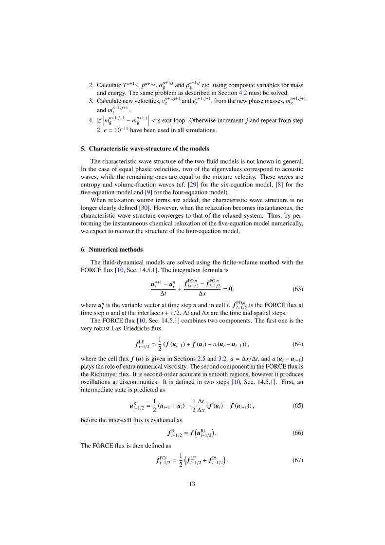
Liquid

Figure 2: Speed of sound, c, plotted against gas volume fraction, αg, at T = 270 K andP = 3.2033 MPa (saturation pressure at T = 270 K).

7. Numerical results

In the current section, we present numerical results for the four-equation and five-equation two-fluid models. A shock tube case is used to study the resolution of the wavepropagation. A moving Gauss curve test case is presented to show the convergence or-der in smooth regions. It is also used to assess the performance of the two approaches interms of computational time. A volume-fraction discontinuity propagating at constantvelocity in a constant pressure field is used to test if the numerical scheme producespressure and velocity oscillations at the discontinuity. A separation case shows how thefour-equation model handles the transition to single-phase flow. Further, a two-phaseexpansion tube is used to simulate cavitation and expansion waves in the presence ofequilibrium mass transfer. The volume-fraction discontinuity and the separation caseare only simulated using the four-equation model.

For equation (9) the value δ = 2 has been used in all simulations.

7.1. Speed of sound estimatesFigure 2 shows the speed of sound for the five-equation and four-equation models,

plotted against the gas volume fraction at T = 270 K and P = 3.2033 MPa. Thespeed of sound assuming phase equilibrium, cTF4 (48), is generally lower than the non-equilibrium speed of sound cTF5 (14). Note also that the speed of sound assuming fullequilibrium is discontinuous at the transition to single phase. For example, the speedof sound in the liquid is close to 600 m/s, but with the first bubble appearing, it dropsto under 50 m/s. This behaviour has already been noted in [20].

7.2. Shock tubeA shock tube is a case in which two constant states are separated by a single dis-

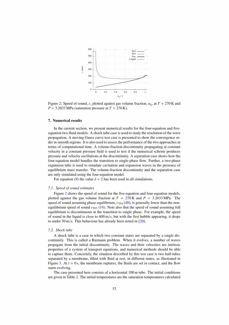
continuity. This is called a Riemann problem. When it evolves, a number of wavespropagate from the initial discontinuity. The waves and their velocities are intrinsicproperties of a system of transport equations, and numerical methods should be ableto capture them. Concretely, the situation described by this test case is two half-tubesseparated by a membrane, filled with fluid at rest, in different states, as illustrated inFigure 3. At t = 0 s, the membrane ruptures, the fluids are set in contact, and the flowstarts evolving.

The case presented here consists of a horizontal 100 m tube. The initial conditionsare given in Table 2. The initial temperatures are the saturation temperatures calculated

15

αLg , vL

g , vL`

pL, T L

αRg , vR

g , vR`

pR, T R

Figure 3: Shock tube.

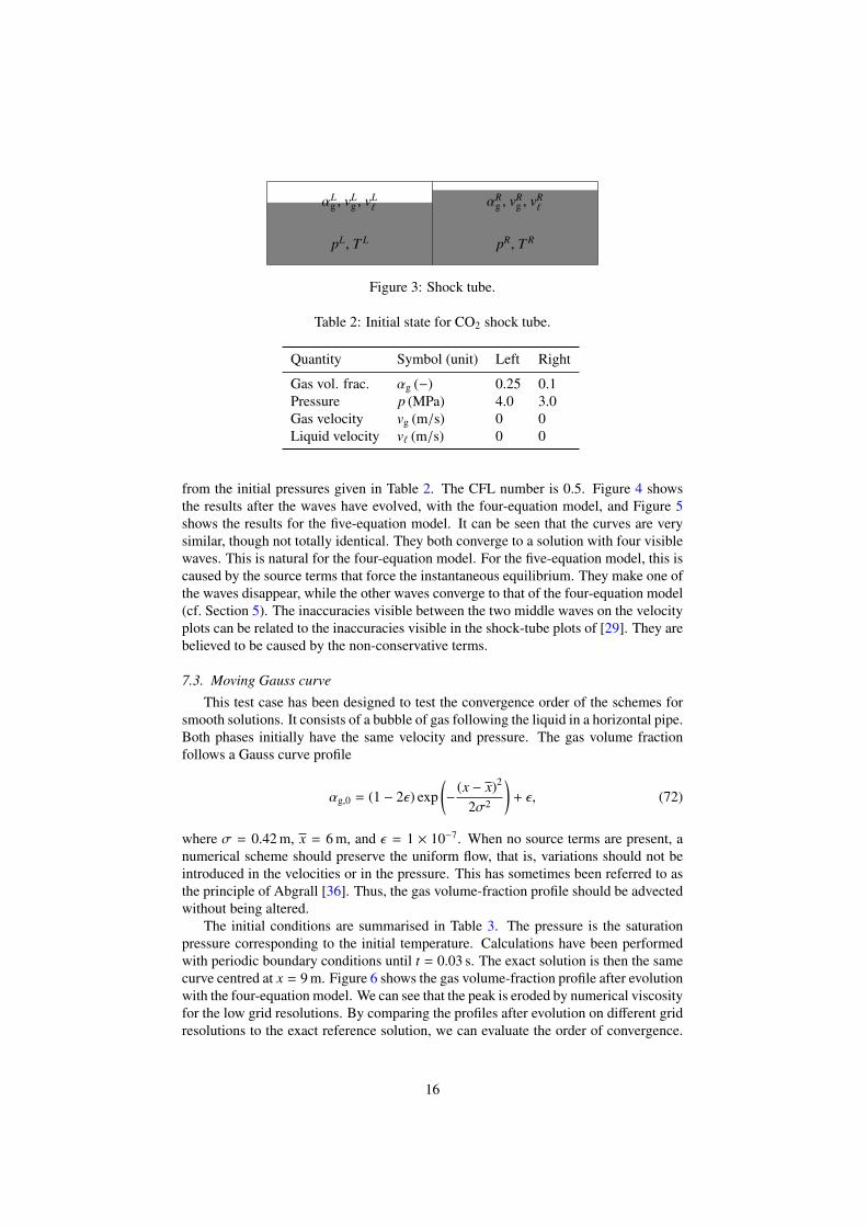
Table 2: Initial state for CO2 shock tube.

Quantity Symbol (unit) Left Right

Gas vol. frac. αg (−) 0.25 0.1Pressure p (MPa) 4.0 3.0Gas velocity vg (m/s) 0 0Liquid velocity v` (m/s) 0 0

from the initial pressures given in Table 2. The CFL number is 0.5. Figure 4 showsthe results after the waves have evolved, with the four-equation model, and Figure 5shows the results for the five-equation model. It can be seen that the curves are verysimilar, though not totally identical. They both converge to a solution with four visiblewaves. This is natural for the four-equation model. For the five-equation model, this iscaused by the source terms that force the instantaneous equilibrium. They make one ofthe waves disappear, while the other waves converge to that of the four-equation model(cf. Section 5). The inaccuracies visible between the two middle waves on the velocityplots can be related to the inaccuracies visible in the shock-tube plots of [29]. They arebelieved to be caused by the non-conservative terms.

7.3. Moving Gauss curve

This test case has been designed to test the convergence order of the schemes forsmooth solutions. It consists of a bubble of gas following the liquid in a horizontal pipe.Both phases initially have the same velocity and pressure. The gas volume fractionfollows a Gauss curve profile

αg,0 = (1 − 2ε) exp(−

(x − x)2

2σ2

)+ ε, (72)

where σ = 0.42 m, x = 6 m, and ε = 1 × 10−7. When no source terms are present, anumerical scheme should preserve the uniform flow, that is, variations should not beintroduced in the velocities or in the pressure. This has sometimes been referred to asthe principle of Abgrall [36]. Thus, the gas volume-fraction profile should be advectedwithout being altered.

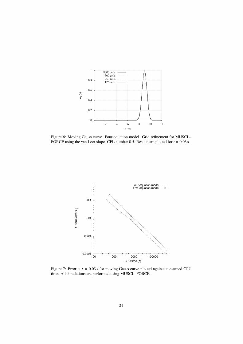
The initial conditions are summarised in Table 3. The pressure is the saturationpressure corresponding to the initial temperature. Calculations have been performedwith periodic boundary conditions until t = 0.03 s. The exact solution is then the samecurve centred at x = 9 m. Figure 6 shows the gas volume-fraction profile after evolutionwith the four-equation model. We can see that the peak is eroded by numerical viscosityfor the low grid resolutions. By comparing the profiles after evolution on different gridresolutions to the exact reference solution, we can evaluate the order of convergence.

16

0

0.05

0.1

0.15

0.2

0.25

0.3

0.35

0.4

0 20 40 60 80 100

αg

(-)

x (m)

10000 cells5000 cells2500 cells1250 cells

(a) Gas volume fraction.

0

50

100

150

200

250

300

350

400

0 20 40 60 80 100

vg

(m/s

)

x (m)

10000 cells5000 cells2500 cells1250 cells

(b) Gas velocity.

0

1

2

3

4

5

6

7

8

0 20 40 60 80 100

v`

(m/s

)

x (m)

10000 cells5000 cells2500 cells1250 cells

(c) Liquid velocity.

3

3.2

3.4

3.6

3.8

4

0 20 40 60 80 100

p(M

Pa)

x (m)

10000 cells5000 cells2500 cells1250 cells

(d) Pressure.

266

268

270

272

274

276

278

280

0 20 40 60 80 100

T(K

)

x (m)

10000 cells5000 cells2500 cells1250 cells

(e) Temperature.

Figure 4: CO2 shock tube solved using the four-equation model. Result at t = 0.15 susing the CFL number 0.5. The Riemann problem is solved using the FORCE flux.

Table 3: Initial state for the moving Gauss curve.

Quantity Symbol (unit) Value

Gas vol. frac. αg (−) αg,0(x)Pressure p (MPa) 3.2033 (sat. pres.)Temperature T (K) 270Gas velocity vg (m/s) 100Liquid velocity v` (m/s) 100

17

0

0.05

0.1

0.15

0.2

0.25

0.3

0.35

0.4

0 20 40 60 80 100

αg

(-)

x (m)

10000 cells5000 cells2500 cells1250 cells

(a) Gas volume fraction.

0

50

100

150

200

250

300

350

400

0 20 40 60 80 100

vg

(m/s

)x (m)

10000 cells5000 cells2500 cells1250 cells

(b) Gas velocity.

0

1

2

3

4

5

6

7

8

0 20 40 60 80 100

v`

(m/s

)

x (m)

10000 cells5000 cells2500 cells1250 cells

(c) Liquid velocity.

3

3.2

3.4

3.6

3.8

4

0 20 40 60 80 100

p(M

Pa)

x (m)

10000 cells5000 cells2500 cells1250 cells

(d) Pressure.

266

268

270

272

274

276

278

280

0 20 40 60 80 100

T(K

)

x (m)

10000 cells5000 cells2500 cells1250 cells

(e) Temperature.

Figure 5: CO2 shock tube solved using the five-equation model. Result at t = 0.15 susing the CFL number 0.5. The Riemann problem is solved using the FORCE flux.

18

Table 4: Moving Gauss curve simulated using MUSCL-FORCE and second order RKtime integration. Convergence order, sN , and 1–norm of the error in the gas volumefraction by grid refinement.

TF4 MUSCL-FORCE TF5 MUSCL-FORCEN(−) ‖E(αg)‖1 sN ‖E(αg)‖1 sN125 1.1412 × 10−1 − 2.0145 × 10−1 −

250 2.9719 × 10−2 1.94 5.2551 × 10−2 1.94500 8.0421 × 10−3 1.89 1.2690 × 10−2 2.051000 2.0530 × 10−3 1.97 3.0749 × 10−3 2.052000 4.9704 × 10−4 2.05 7.2381 × 10−4 2.094000 1.1913 × 10−4 2.06 1.6809 × 10−4 2.108000 2.8316 × 10−5 2.07 3.8658 × 10−5 2.12

Table 5: Moving Gauss curve simulated using the FORCE flux and forward Euler intime. Convergence order, sN , and 1–norm of the error in the gas volume fraction bygrid refinement.

TF4 FORCE TF5 FORCEN(−) ‖E(αg)‖1 sN ‖E(αg)‖1 sN125 7.2185 × 10−1 − 1.1211 −

250 5.1865 × 10−1 0.477 8.8405 × 10−1 0.343500 3.4618 × 10−1 0.583 6.4475 × 10−1 0.4551000 2.1362 × 10−1 0.696 4.2957 × 10−1 0.5862000 1.2288 × 10−1 0.798 2.6186 × 10−1 0.7144000 6.6949 × 10−2 0.876 1.4822 × 10−1 0.8218000 3.5146 × 10−2 0.930 7.9587 × 10−2 0.897

The error in the calculated gas volume fraction at a given time step has been quantifiedusing the 1-norm

‖E(αg)‖1 = ∆x∑∀ j

|αg, j − αg,ref, j|, (73)

where j is the cell index and the subscript “ref” indicates the exact reference solution.Then, the convergence order sN for a number of cells N is estimated by

sN =

ln(‖E(αg)‖1,N‖E(αg)‖1,N/2

)ln 2

. (74)

Table 4 shows the results for the four-equation and five-equation models. As expectedfor the MUSCL-FORCE scheme, the convergence order is close to 2, since the solutionis smooth. Here, the van Leer [11], limiter has been used.

Table 5 shows the results for the four-equation and five-equation models with theFORCE scheme. The convergence order is approaching 1.

The relevant comparison to evaluate the efficiency of a method is to compare theerror in the solution to the CPU time used to arrive at the solution. The advantageof the five-equation-based approach is that the flashing problem is independent ofthe fluid-dynamical problem, thus simplifying the solution procedure. In the four-equation-based approach, the flashing problem and the kinetic energy problem must be

19

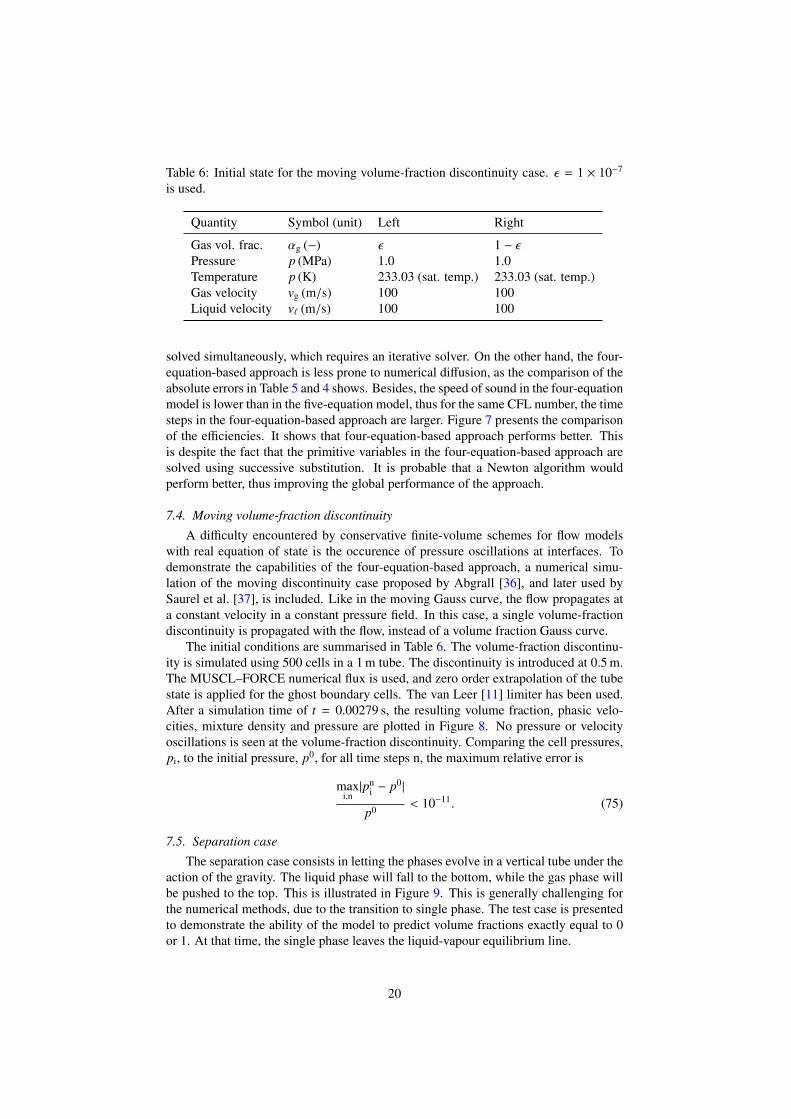
Table 6: Initial state for the moving volume-fraction discontinuity case. ε = 1 × 10−7

is used.

Quantity Symbol (unit) Left Right

Gas vol. frac. αg (−) ε 1 − εPressure p (MPa) 1.0 1.0Temperature p (K) 233.03 (sat. temp.) 233.03 (sat. temp.)Gas velocity vg (m/s) 100 100Liquid velocity v` (m/s) 100 100

solved simultaneously, which requires an iterative solver. On the other hand, the four-equation-based approach is less prone to numerical diffusion, as the comparison of theabsolute errors in Table 5 and 4 shows. Besides, the speed of sound in the four-equationmodel is lower than in the five-equation model, thus for the same CFL number, the timesteps in the four-equation-based approach are larger. Figure 7 presents the comparisonof the efficiencies. It shows that four-equation-based approach performs better. Thisis despite the fact that the primitive variables in the four-equation-based approach aresolved using successive substitution. It is probable that a Newton algorithm wouldperform better, thus improving the global performance of the approach.

7.4. Moving volume-fraction discontinuity

A difficulty encountered by conservative finite-volume schemes for flow modelswith real equation of state is the occurence of pressure oscillations at interfaces. Todemonstrate the capabilities of the four-equation-based approach, a numerical simu-lation of the moving discontinuity case proposed by Abgrall [36], and later used bySaurel et al. [37], is included. Like in the moving Gauss curve, the flow propagates ata constant velocity in a constant pressure field. In this case, a single volume-fractiondiscontinuity is propagated with the flow, instead of a volume fraction Gauss curve.

The initial conditions are summarised in Table 6. The volume-fraction discontinu-ity is simulated using 500 cells in a 1 m tube. The discontinuity is introduced at 0.5 m.The MUSCL–FORCE numerical flux is used, and zero order extrapolation of the tubestate is applied for the ghost boundary cells. The van Leer [11] limiter has been used.After a simulation time of t = 0.00279 s, the resulting volume fraction, phasic velo-cities, mixture density and pressure are plotted in Figure 8. No pressure or velocityoscillations is seen at the volume-fraction discontinuity. Comparing the cell pressures,pi, to the initial pressure, p0, for all time steps n, the maximum relative error is

maxi,n|pn

i − p0|

p0 < 10−11. (75)

7.5. Separation case

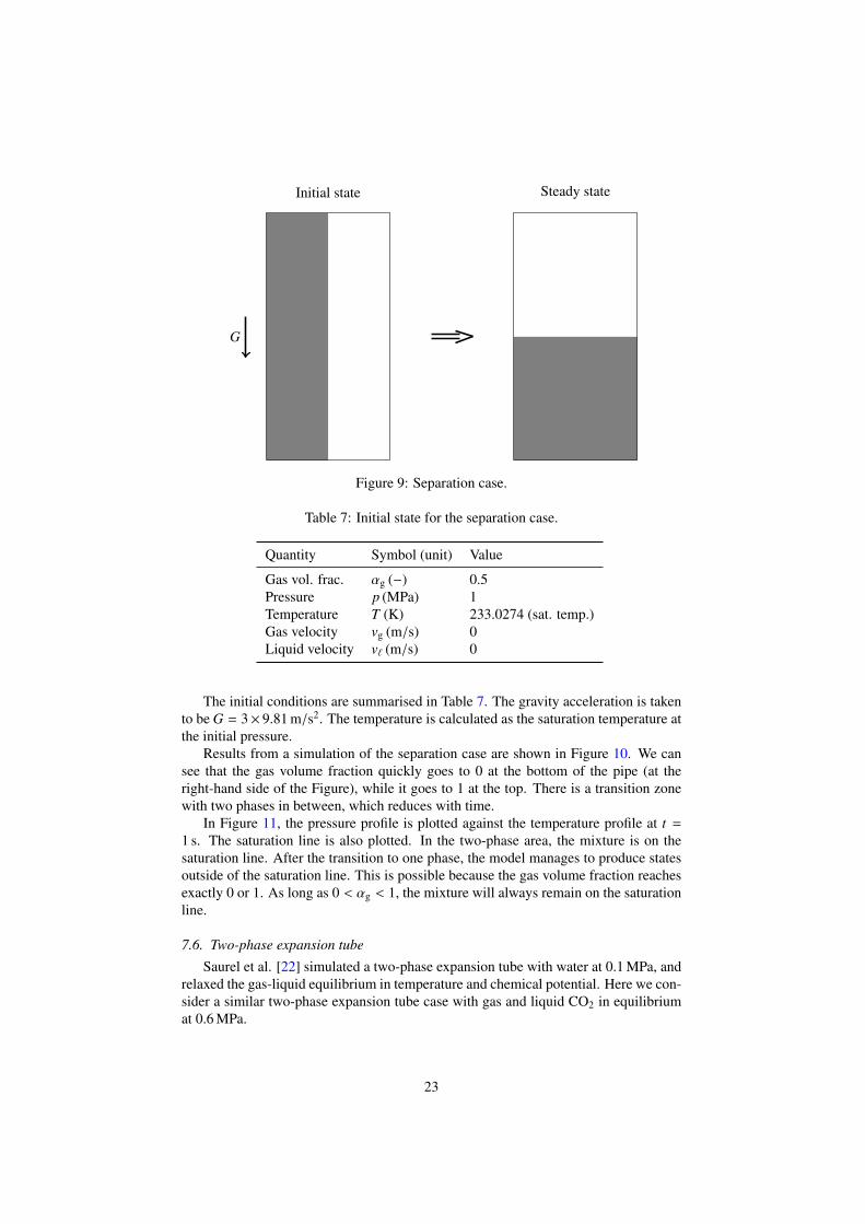
The separation case consists in letting the phases evolve in a vertical tube under theaction of the gravity. The liquid phase will fall to the bottom, while the gas phase willbe pushed to the top. This is illustrated in Figure 9. This is generally challenging forthe numerical methods, due to the transition to single phase. The test case is presentedto demonstrate the ability of the model to predict volume fractions exactly equal to 0or 1. At that time, the single phase leaves the liquid-vapour equilibrium line.

20

0

0.2

0.4

0.6

0.8

1

0 2 4 6 8 10 12

αg

(-)

x (m)

8000 cells500 cells250 cells125 cells

Figure 6: Moving Gauss curve. Four-equation model. Grid refinement for MUSCL–FORCE using the van Leer slope. CFL number 0.5. Results are plotted for t = 0.03 s.

0.0001

0.001

0.01

0.1

1

100 1000 10000 100000

1-N

orm

err

or

(-)

CPU time (s)

Four-equation modelFive-equation model

Figure 7: Error at t = 0.03 s for moving Gauss curve plotted against consumed CPUtime. All simulations are performed using MUSCL–FORCE.

21

0

0.2

0.4

0.6

0.8

1

0 0.2 0.4 0.6 0.8 1

αg

(-)

x (m)

Reference500 cells

(a) Gas volume fraction.

99

99.5

100

100.5

101

0 0.2 0.4 0.6 0.8 1

v(m

/s)

x (m)

vgv`

(b) Gas and liquid velocity.

0

200

400

600

800

1000

1200

0 0.2 0.4 0.6 0.8 1

ρm

( kg/m

3)

x (m)

Reference500 cells

(c) Mixture density.

0.99

0.995

1

1.005

1.01

0 0.2 0.4 0.6 0.8 1

p(M

Pa)

x (m)

Reference500 cells

(d) Pressure.

Figure 8: Moving volume-fraction discontinuity using the four-equation model. Resultat t = 0.00279 s using CFL number 0.5 and 500 cells are plotted together with thereference solution. Reference solutions for the velocities, vg = v` = 100 m/s , areomitted. The Riemann problem is solved using MUSCL–FORCE flux.

22

Initial state Steady state

G

Figure 9: Separation case.

Table 7: Initial state for the separation case.

Quantity Symbol (unit) Value

Gas vol. frac. αg (−) 0.5Pressure p (MPa) 1Temperature T (K) 233.0274 (sat. temp.)Gas velocity vg (m/s) 0Liquid velocity v` (m/s) 0

The initial conditions are summarised in Table 7. The gravity acceleration is takento be G = 3× 9.81 m/s2. The temperature is calculated as the saturation temperature atthe initial pressure.

Results from a simulation of the separation case are shown in Figure 10. We cansee that the gas volume fraction quickly goes to 0 at the bottom of the pipe (at theright-hand side of the Figure), while it goes to 1 at the top. There is a transition zonewith two phases in between, which reduces with time.

In Figure 11, the pressure profile is plotted against the temperature profile at t =

1 s. The saturation line is also plotted. In the two-phase area, the mixture is on thesaturation line. After the transition to one phase, the model manages to produce statesoutside of the saturation line. This is possible because the gas volume fraction reachesexactly 0 or 1. As long as 0 < αg < 1, the mixture will always remain on the saturationline.

7.6. Two-phase expansion tube

Saurel et al. [22] simulated a two-phase expansion tube with water at 0.1 MPa, andrelaxed the gas-liquid equilibrium in temperature and chemical potential. Here we con-sider a similar two-phase expansion tube case with gas and liquid CO2 in equilibriumat 0.6 MPa.

23

0

0.2

0.4

0.6

0.8

1

0 1.5 3 4.5 6 7.5

αg

(-)

x (m)

t = 0.0st = 0.1st = 0.2st = 0.3st = 0.4st = 0.5st = 1.0s

Figure 10: Separation case. The four equation model and the FORCE scheme is appliedwith CFL number 0.5, and 4000 cells. The gas volume fraction, αg, profile is plottedat 7 different times.

0.92

0.94

0.96

0.98

1

1.02

1.04

232.25 232.5 232.75 233 233.25

P(M

Pa)

T (K)

Saturation linet = 1.0s

Figure 11: Separation case pressure plotted versus temperature at t = 1.0 s. The satur-ation pressure is also plotted, to illustrate where the the transition to single phase. Thecase is simulated using FORCE, CFL number 0.5, and 4000 cells.

24

Table 8: Initial state for the two-phase CO2 expansion tube.

Quantity Symbol (unit) Left Right

Gas vol. frac. αg (−) 0.01 0.01Pressure p (MPa) 0.6 0.6Temperature p (K) 220.0 220.0Gas velocity vg (m/s) −2.0 2.0Liquid velocity v` (m/s) −2.0 2.0Gas density ρg (kg/m3) 15.839 15.839Liquid density ρ` (kg/m3) 1154.6 1154.6

Initially a 1 m long tube contains 1 % gas, αg = 0.01, uniformly distributed. Loc-ated at x = 0.5 m there is a velocity discontinuity. On the left side the velocity is set toug = u` = −2.0 m/s, and on the right side the velocity is set to ug = u` = 2.0 m/s. Theinital conditions are summarised in Table 8.

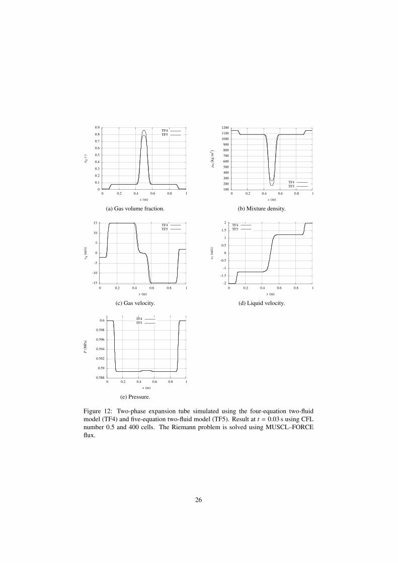
The MUSCL–FORCE numerical flux is used, and zero order extrapolation of thetube state is applied for the ghost boundary cells. The van Leer [11] limiter has beenused. After a simulation time of t = 0.03 s, the resulting gas volume fraction, phasicvelocites, mixture density and pressure are plotted in Figure 12. A CFL number of 0.5was used.

Figure 12 shows one rarefaction wave traveling to the left and one to the right.These leading expansion waves are followed by two slower evaporation fronts. Atx = 0.5 m a cavitation pocket forms, where the gas volume fraction become close to1. The gas volume fraction increase due to gas expansion, phase transfer and partlyby inflow of gas. Even if the two-phase expansion tube is simulated with CO2 at fullequilibrium, and at different conditions than by Saurel et al. [22], the same waves andthe same qualitative behaviour is seen. From Figure 12a and 12b, it is seen that thefive-equation model gives larger numerical diffusion than the four-equation model.

8. Summary

In the present work, we have numerically compared approaches to solve two differ-ent two-fluid models using a real equation of state, when assuming full thermodynamicequilibrium between the phases. The Span-Wagner reference equation of state for CO2is used to describe phase equilibrium and thermodynamic properties.

The first approach consists in letting the flow evolve first without mass transfer,and then correct the solution to an equilibrium state using a fractional-step method. Inthis case the two-fluid model consists of two mass, two momentum and one energyequation. The second approach ensures thermodynamic phase equilibrium at all times,reducing the model from two to only one mass equation.

The five-equation model only involves equilibrium in pressure and temperature,thus its speed of sound is continuous in the transition to single phase. The full thermo-dynamic equilibrium assumption gives a discontinuous speed of sound in the transitionbetween single and two-phase flow. The mixture speed of sound in the four-equationmodel is generally lower than the mixture speed of sound in the five-equation model.

The four-equation model introduced additional complexity in the calculation of theprimitive variables from conserved quantities. The kinetic energy is constant during

25

0

0.1

0.2

0.3

0.4

0.5

0.6

0.7

0.8

0.9

0 0.2 0.4 0.6 0.8 1

αg

(-)

x (m)

TF4TF5

(a) Gas volume fraction.

100

200

300

400

500

600

700

800

900

1000

1100

1200

0 0.2 0.4 0.6 0.8 1

ρm

( kg/m

3)x (m)

TF4TF5

(b) Mixture density.

-15

-10

-5

0

5

10

15

0 0.2 0.4 0.6 0.8 1

v g(m

/s)

x (m)

TF4TF5

(c) Gas velocity.

-2

-1.5

-1

-0.5

0

0.5

1

1.5

2

0 0.2 0.4 0.6 0.8 1

v `(m

/s)

x (m)

TF4TF5

(d) Liquid velocity.

0.588

0.59

0.592

0.594

0.596

0.598

0.6

0 0.2 0.4 0.6 0.8 1

P(M

Pa)

x (m)

TF4TF5

(e) Pressure.

Figure 12: Two-phase expansion tube simulated using the four-equation two-fluidmodel (TF4) and five-equation two-fluid model (TF5). Result at t = 0.03 s using CFLnumber 0.5 and 400 cells. The Riemann problem is solved using MUSCL–FORCEflux.

26

mass transfer with the fractional-step approach, but had to be determined by iterationin the four-equation model.

Second-order convergence is achieved for both models on a Gauss curve shapedvolume-fraction wave advected in a constant flow field. The FORCE scheme andMUSCL with van Leer limiter together with a two-stage second-order strong-stability-preserving Runge–Kutta time integration was applied. The second-order MUSCL-FORCE scheme for both the four- and five-equation models also performed well onthe discontinuous solutions of a shock tube.

Applying the four-equation model on a volume-fraction discontinuity propagatingat constant velocity in an constant pressure field, no pressure or velocity oscillationswere seen at the discontinuity.

A numerical test of a two-phase CO2 expansion tube is performed applying both thefour-equation and five-equation two-fluid model. The initial velocity discontinuity pro-duces the same four expansion waves, the cavitation pocket, and the same qualitativebehaviour is seen in the results as in the numerical example by Saurel et al. [22]. Thenumerical diffusion when solving the five-equation model is larger than when solvingthe four-equation model.

Mainly due to a larger time step in the four-equation model, the performance of thefour-equation model was shown to be superior to that of the five-equation model. Theperformance was quantified as solution error per CPU time consumed.

To demonstrate the ability of the approach to handle transition from two-phase flowto single-phase flow, the four-equation model was applied to a separation case, wheregravity separates an initially homogenous mixture of gas and liquid. By plotting thesimulated pressure against temperature together with the CO2 saturation line, gas-liquidtransition to pure liquid was verified.

Acknowledgments

This work was supported by the CO2 Dynamics project. The authors acknowledgethe support from the Research Council of Norway (189978), Gassco AS, Statoil Petro-leum AS and Vattenfall AB. We are grateful to our colleague Svend Tollak Munkejord,Tore Flåtten and Peder Aursand, for fruitful discussions.

27

References

[1] IEA, Energy Technology Perspectives, 2012. doi:10.1787/20792603.

[2] R. Saurel, R. Abgrall, A multiphase Godunov method for compressible multifluidand multiphase flow, J. Comput. Phys. 150 (2) (1999) 425–467.

[3] R. Saurel, O. Le Métayer, A multiphase model for compressible flows with inter-faces, shocks, detonation waves and cavitation, J. Fluid Mech. 431 (2001) 239–271.

[4] H. Paillère, C. Corre, J. R. García Cascales, On the extension of the AUSM+

scheme to compressible two-fluid models, Comput. Fluids 32 (6) (2003) 891–916.

[5] O. Le Métayer, J. Massoni, R. Saurel, Elaborating equations of state of a liquidand its vapor for two-phase flow models, Int. J. Therm. Sci. 43 (3) (2004) 265–276.

[6] H. O. Nordhagen, S. Kragset, T. Berstad, A. Morin, C. Dørum, S. T. Munkejord,A new coupled fluid-structure modelling methodology for running ductile frac-ture, Comput. Struct. 94–95 (2012) 13–21. doi:10.1016/j.compstruc.2012.01.004.

[7] R. Span, W. Wagner, A new equation of state for carbon dioxide covering the fluidregion from the triple-point temperature to 1100 K at pressures up to 800 MPa, J.Phys. Chem. Ref. Data 25 (6) (1996) 1509–1596. doi:10.1063/1.555991.

[8] P. J. Martínez Ferrer, T. Flåtten, S. T. Munkejord, On the effect of temperatureand velocity relaxation in two-phase flow models, ESAIM – Math. Model. Num.46 (2) (2012) 411–442. doi:10.1051/m2an/2011039.

[9] A. Morin, T. Flåtten, A two-fluid four-equation model with instantaneous thermo-dynamical equilibrium, Submitted for publication 2013. Preprint available fromhttp://www.math.ntnu.no/conservation/2013/002.html.

[10] E. F. Toro, Riemann solvers and numerical methods for fluid dynamics, 2nd Edi-tion, Springer-Verlag, Berlin, 1999.

[11] B. van Leer, Towards the ultimate conservative difference scheme V. A second-order sequel to Godunov’s method, J. Comput. Phys. 32 (1) (1979) 101–136.

[12] M. Ishii, Thermo-fluid dynamic theory of two-phase flow, Collection de la Direc-tion des Etudes et Recherches d’Electricité de France, Eyrolles, Paris, 1975.

[13] S. T. Munkejord, S. Evje, T. Flåtten, A MUSTA scheme for a nonconservat-ive two-fluid model, SIAM J. Sci. Comput. 31 (4) (2009) 2587–2622. doi:10.1137/080719273.

[14] H. B. Stewart, B. Wendroff, Review article: Two-phase flow: Models and meth-ods, J. Comput. Phys. 56 (3) (1984) 363–409.

[15] I. Toumi, A. Kumbaro, An approximate linearized Riemann solver for a two-fluidmodel, J. Comput. Phys. 124 (2) (1996) 286–300.

28

[16] D. Bestion, The physical closure laws in the CATHARE code, Nucl. Eng. Design124 (3) (1990) 229–245.

[17] V. H. Ransom et. al., RELAP5/MOD3 Code Manual, NUREG/CR-5535, IdahoNational Engineering Laboratory, ID (1995).

[18] K. H. Bendiksen, D. Malnes, R. Moe, S. Nuland, The dynamic two-fluid modelOLGA: Theory and application, SPE Production Engineering 6 (2) (1991) 171–180.

[19] J. H. Stuhmiller, The influence of interfacial pressure forces on the character oftwo-phase flow model equations, Int. J. Multiphase Flow 3 (6) (1977) 551–560.

[20] T. Flåtten, H. Lund, Relaxation two-phase flow models and the subcharacteristiccondition, Math. Mod. Meth. Appl. S. 21 (12) (2011) 2379–2407. doi:10.1142/S0218202511005775.

[21] H. Lund, A hierarchy of relaxation models for two-phase flow, SIAM J. Appl.Math. 72 (6) (2012) 1713–1741. doi:10.1137/12086368X.

[22] R. Saurel, F. Petitpas, R. Abgrall, Modelling phase transition in metastable li-quids: application to cavitating and flashing flows, J. Fluid Mech. 607 (2008)313–350. doi:10.1017/S0022112008002061.

[23] H. Bruce Stewart, B. Wendroff, Two-phase flow: models and methods, J. Comput.Phys. 56 (3) (1984) 363–409.

[24] R. J. LeVeque, Finite Volume Methods for Hyperbolic Problems, Cambridge Uni-versity Press, Cambridge, UK, 2002.

[25] F. Coquel, K. El Amine, E. Godlewski, B. Perthame, P. Rascle, A numericalmethod using upwind schemes for the resolution of two-phase flows, J. Comput.Phys. 136 (2) (1997) 272–288.

[26] M. L. Michelsen, State function based flash specifications, Fluid Phase Equilib.158-160 (1999) 617 – 626. doi:10.1016/S0378-3812(99)00092-8.

[27] K. E. T. Giljarhus, S. T. Munkejord, G. Skaugen, Solution of the Span-Wagnerequation of state using a density-energy state function for fluid-dynamic sim-ulation of carbon dioxide, Ind. Eng. Chem. Res. 51 (2) (2012) 1006–1014.doi:10.1021/ie201748a.

[28] M. Hammer, Å. Ervik, S. T. Munkejord, Method using a density-energy statefunction with a reference equation of state for fluid-dynamics simulation of vapor-liquid-solid carbon dioxide, Ind. Eng. Chem. Res. 52 (29) (2013) 9965–9978.doi:10.1021/ie303516m.

[29] A. Morin, T. Flåtten, S. T. Munkejord, A Roe scheme for a compressible six-equation two-fluid model, Int. J. Numer. Meth. Fl. 72 (2013) 478–504.

[30] P. Aursand, T. Flåtten, On the dispersive wave-dynamics of 2 × 2 relaxationsystems, J. Hyperbolic Differ. Equ. 9 (4) (2012) 641–659. doi:10.1142/S021989161250021X.

29

[31] S. Osher, Convergence of generalized MUSCL schemes, SIAM J. Numer. Anal.22 (5) (1985) 947–961.

[32] D. I. Ketcheson, A. C. Robinson, On the practical importance of the SSP propertyfor Runge-Kutta time integrators for some common Godunov-type schemes, Int.J. Numer. Meth. Fl. 48 (3) (2005) 271–303.

[33] R. Abgrall, S. Karni, Comment on the computation of non-conservative products,J. Comput. Phys. 229 (8) (2010) 2759–2763. doi:10.1016/j.jcp.2009.12.015.

[34] M. J. Castro, P. G. LeFloch, M. L. Muñoz-Ruiz, C. Parés, Why many theor-ies of shock waves are necessary: Convergence error in formally path-consistentschemes, J. Comput. Phys. 227 (17) (2008) 8107–8129. doi:10.1016/j.jcp.2008.05.012.

[35] G. Dal Maso, P. G. LeFloch, F. Murat, Definition and weak stability of noncon-servative products, J. Math. Pures Appl. 74 (6) (1995) 483–548.

[36] R. Abgrall, How to prevent pressure oscillations in multicomponent flow calcula-tions: A quasi conservative approach, J. Comput. Phys. 125 (1) (1996) 150–160.

[37] R. Saurel, F. Petitpas, R. A. Berry, Simple and efficient relaxation meth-ods for interfaces separating compressible fluids, cavitating flows and shocksin multiphase mixtures, J. Comput. Phys. 228 (5) (2009) 1678–1712,10.1016/j.jcp.2008.11.002.

30