a meshless method for the stable solution of singular inverse problems for two-dimensional...

ARTICLE IN PRESS

Engineering Analysis with Boundary Elements 34 (2010) 274–288

Contents lists available at ScienceDirect

Engineering Analysis with Boundary Elements

0955-79

doi:10.1

� Tel./

E-m

journal homepage: www.elsevier.com/locate/enganabound

A meshless method for the stable solution of singular inverse problems fortwo-dimensional Helmholtz-type equations

Liviu Marin �

Institute of Solid Mechanics, Romanian Academy, 15 Constantin Mille, Sector 1, P.O. Box 1-863, 010141 Bucharest, Romania

a r t i c l e i n f o

Article history:

Received 6 January 2009

Accepted 7 March 2009Available online 17 October 2009

Keywords:

Helmholtz-type equations

Singular inverse problems

Singularity subtraction technique (SST)

Regularization

Method of fundamental solutions (MFS)

97/$ - see front matter & 2009 Elsevier Ltd. A

016/j.enganabound.2009.03.009

fax: +40 (0) 21312 6736.

ail addresses: [email protected], liviu@im

a b s t r a c t

We investigate a meshless method for the stable and accurate solution of inverse problems associated

with two-dimensional Helmholtz-type equations in the presence of boundary singularities. The

governing equation and boundary conditions are discretized by the method of fundamental solutions

(MFS). The existence of boundary singularities affects adversely the accuracy and convergence of

standard numerical methods. Solutions to such problems and/or their corresponding derivatives may

have unbounded values in the vicinity of the singularity. Moreover, when dealing with inverse

problems, the stability of solutions is a key issue and this is usually taken into account by employing a

regularization method. These difficulties are overcome by combining the Tikhonov regularization

method (TRM) with the subtraction from the original MFS solution of the corresponding singular

solutions, without an appreciable increase in the computational effort and at the same time keeping the

same MFS discretization. Three examples for both the Helmholtz and the modified Helmholtz equations

are carefully investigated.

& 2009 Elsevier Ltd. All rights reserved.

1. Introduction

Helmholtz-type equations are often used to describe theacoustic cavity problem [1], the heat conduction in fins [2], thevibration of a structure [3], the radiation wave [4] and thescattering of a wave [5]. In many engineering problems governedby Helmholtz-type equations, boundary singularities arise whenthere are sharp re-entrant corners in the boundary, the boundaryconditions change abruptly, or there are discontinuities in thematerial properties. It is well known that these situations give riseto singularities of various types and, as a consequence, thesolutions to such problems and/or their corresponding derivativesmay have unbounded values in the vicinity of the singularity.Singularities are known to affect adversely the accuracy andconvergence of standard numerical methods, such as finiteelement (FEM), boundary element (BEM), finite-difference(FDM), spectral and meshless/meshfree methods. If, however,the form of the singularity is taken into account and is properlyincorporated into the numerical scheme then a more effectivemethod may be constructed.

There are important studies regarding the numerical treatmentof singularities in Helmholtz-type equations, see e.g. [3–11]. Chenet al. [3] analysed time-harmonic waves in a membrane whichcontains one or more fixed edge stringers or cracks by using the

ll rights reserved.

sar.bu.edu.ro.

dual BEM. Huang et al. [4] investigated the electromagnetic fielddue to a line source radiating in the presence of a two-dimensional composite wedge made of a number of conductingand dielectric materials by employing the Fourier transform pathintegral method. A hybrid asymptotic/FEM for computing theacoustic field radiated or scattered by acoustically large objectswas developed by Barbone et al. [5]. The method of the auxiliarymapping and the p-version of the FEM were employed by Cai et al.[6] and Lucas and Oh [7] to remove the pollution effect caused bysingularities in the Helmholtz equation. Wu and Han [8] solvedsingular boundary value problems for both Laplace and Helm-holtz-type equations by using the FEM and introducing asequence of approximations to the boundary conditions at anartificial boundary. Xu and Chen [9] used the FDM and higher-order discretized boundary conditions at the edges of perfectlyconducting wedges for TE waves to retrieve accurately the fieldbehaviour near a sharp edge. The treatment of singularities inboth isotropic and anisotropic two-dimensional Helmholtz-typeequations was investigated by Marin et al. [10], who modified thestandard BEM to account for the presence of singularities. For anexcellent survey on the treatment of singularities in ellipticboundary value problems, we refer the reader to Li and Lu [11] andthe references therein.

The method of fundamental solutions (MFS) is a meshless/meshfree boundary collocation method which is applicable toboundary value problems for which a fundamental solution ofthe operator in the governing equation is known. In spite of thisrestriction, it has, in recent years, become very popular primarily

www.elsevier.com/locate/enganabound

dx.doi.org/10.1016/j.enganabound.2009.03.009

mailto:[email protected]

mailto:[email protected]

ARTICLE IN PRESS

L. Marin / Engineering Analysis with Boundary Elements 34 (2010) 274–288 275

because of the ease with which it can be implemented, inparticular for problems in complex geometries. Since itsintroduction as a numerical method by Mathon and Johnston[12], it has been successfully applied to a large variety of physicalproblems, an account of which may be found in the surveypapers [13–16]. Recently, the MFS has been successfully appliedto solving inverse problems associated with the heat equation[17,18], linear elasticity [19,20], steady-state heat conduction infunctionally graded materials [21], Helmholtz-type equations[22–24], and source reconstruction in steady-state heat conduc-tion problems [25]. Numerous studies in the literature have beendevoted to the application, in a stable manner, of the MFS tosingular problems, see [26–31]. The standard MFS was modifiedin order to take into account the presence of boundarysingularities in both the Laplace and the biharmonic equationsby Karageorghis [26] and Poullikkas et al. [27], respectively.Karageorghis et al. [28] adapted the MFS formulation toobtaining stable solutions in linear elastic fracture mechanicsproblems involving the opening mode (mode I). Later, Berger etal. [29] extended the method developed in [28] to problemsinvolving not only the opening mode, but the forward shearmode (mode II) as well, and also proposed another solutionmethod based on a domain decomposition approach. Marin [30]applied the MFS, in conjunction with the removal of theassociated singular functions and regularization methods, tothe stable solution of both direct and inverse problems for theLaplace equation subject to noisy boundary data. Recently, thismethod was extended to solving, in a stable manner, directproblems for Helmholtz-type equations, see e.g. Marin [31].

The objective of this paper is to propose, implement andanalyse the MFS for the accurate and stable solution of inverseproblems associated with two-dimensional Helmholtz-typeequations in the presence of boundary singularities. Theexistence of boundary singularities affect adversely the accuracyand convergence of standard numerical methods. Consequently,solutions to such problems and/or their corresponding deriva-tives, which are obtained by a straightforward inversion of theMFS system, may have unbounded values in the vicinity of thesingularity. Moreover, when dealing with inverse problemssubject to noisy data, the stability of solutions becomes a keyissue and this is usually accounted for by employing regulariza-tion methods. These difficulties are overcome by combining theTikhonov regularization method (TRM) with the subtractionfrom the original MFS solution of the corresponding singularsolutions, i.e. using the so-called singularity subtraction techni-que (SST), see e.g. Portela et al. [32], without an appreciableincrease in the computational effort and at the same timekeeping the original MFS discretization. The proposed modifiedMFS is then implemented for inverse problems associated withboth the Helmholtz and the modified Helmholtz equations intwo-dimensional domains with an edge crack or a V-notch, aswell as an L-shaped domain.

2. Mathematical formulation

We assume that the homogeneous Helmholtz-type equation issatisfied in the two-dimensional bounded domain O with apiecewise smooth boundary G¼ @O, such that the potentialsolution and normal flux can be measured on GDlG and GNlG,respectively, where GDa| and GNa|. Moreover, both Dirichletand Neumann data (i.e. Cauchy data) are available on a portionGC ¼GD \ GN of the boundary G, where GCa|, while neither thepotential solution, nor the normal flux can be measured onG\ðGD [ GNÞa| and they have to be determined. Hence the

inverse problem considered recasts as:

DuðxÞ7k2uðxÞ �@2uðxÞ

@x21

þ@2uðxÞ

@x22

7k2uðxÞ ¼ 0; xAO ð1:1Þ

uðxÞ ¼ ~ueðxÞ; xAGD ð1:2Þ

qðxÞ �ruðxÞ � nðxÞ ¼ ~qeðxÞ; xAGN; ð1:3Þ

where kAR, the plus sign corresponds to the Helmholtz equation,while the minus sing is associated with the modified Helmholtzequation, and ~ue

jGDand ~qe

jGNare perturbed prescribed boundary

potential solution and normal flux, respectively, given by

~uejGD¼ ~ujGD

þdu; ~qejGN¼ ~qjGN

þdq: ð2Þ

Here d ~u and d ~q are Gaussian random variables with mean zeroand standard deviations su ¼maxGD

juj � ðpu=100Þ and sq ¼

maxGNjqj � ðpq=100Þ, respectively, generated by the NAG subrou-

tine G05DDF, and pu and pq are the percentages of additive noiseincluded into the exact input data ujGD

and qjGN, respectively, in

order to simulate the inherent measurement errors.In addition, we also assume that the boundary G contains a

singularity at the origin O, which may be caused by a change inthe boundary conditions at the origin and/or a re-entrant corner atthe origin. For the simplicity of the following explanations, weassume that the singularity point is located at the intersection ofthe Dirichlet, GD, and Neumann, GN, boundary parts, i.e.fOg �GD \ GN, where GDa|, GNa|, GD �G, GN �G and wedenote by an overbar the closure of a set, see Fig. 1(a), althoughthe method presented in this paper can easily be extended toother local configurations or boundary conditions.

It is well known that, even for two-dimensional domains withsmooth boundaries, inverse problems are in general considerablymore difficult to solve than direct problems since the solutiondoes not satisfy the general conditions of well-posedness. Moreprecisely, small measurement errors in the input data may resultin very large errors in the solution, see e.g. Hadamard [33].Moreover, the inverse problem under investigation (1.1)–(1.3) isconsiderably more severe than a regular inverse problem, asdescribed above, since the additional singularity amplify theunstable character of the problem. Hence we cannot use a directapproach, such as the least-squares method (LSM), in order tosolve the system of linear equations which arises from thediscretization of the inverse boundary value problem (1.1)–(1.3).

3. Singular solutions for two-dimensional Helmholtz-typeequations

In this section, some well-known results on the solution of thehomogeneous two-dimensional Helmholtz-type equations arerevised. For more details, we refer the reader to Marin et al. [10]and the references therein. For a fixed non-zero complex numberk the homogeneous Helmholtz-type equation in O�R2 can bewritten as

DuðxÞþk2uðxÞ ¼ 0; x¼ ðx1; x2ÞAO: ð3Þ

Note that the values k¼ k and k¼ ik, where kAR, correspond tothe real Helmholtz and modified Helmholtz equations, respec-tively. Let the polar coordinate system ðr; yÞ be defined in the usualway with respect to the Cartesian coordinates ðx1; x2Þ ¼ ðrcosy;rsinyÞ. If we assume that the solution of Eq. (3) in the domain Ocan be written using the separation of variables with respect tothe polar coordinates ðr; yÞ, where r40, then the general solutionof the Helmholtz-type Eq. (3) can be written as

uðr; yÞ ¼ ½g1JlðkrÞþg2NlðkrÞ�½acosðlyÞþbsinðlyÞ�: ð4Þ

ARTICLE IN PRESS

x1

x2

O

A

B

q = q(an)u = u(an)

u = u(an)

q = q(an)

-0.4

-0.2

0.0

0.2

0.4C

D

u = u(an)

q = q(an)

u = ? q = ?

x1

x2O A

B

E

u = u(an)

u = u(an)

u = u(an)

u = u(an)

q = q(an)

C

D-1.0

-0.5

0.0

0.5

1.0

u = u(an)

q = q(an)

u = ? q = ?

x1

x2

OA

B

D

u = u(an)

q = q(an)

u = u(an)

q = q(an)

-0.4

-0.2

0.0

0.2

0.4C

u = u(an)

q = q(an)

u = ? q = ?

D’

-1.0 -0.5 0.0 0.5 1.0

-1.0 -0.5 0.0 0.5 1.0

-1.0 -0.5 0.0 0.5 1.0

Fig. 1. Schematic diagram of the geometry and boundary conditions for

the singular inverse problems investigated, namely: (a) Example 1: N–D

singularity in a domain containing an edge crack OD with y1 ¼ 0 and y2 ¼ p, (b)

Example 2: D–D singularity in an L-shaped domain with y1 ¼ 0 and y2 ¼ 3p=2, and

(c) Example 3: D–N singularity in a domain containing a V-notch with y1 ¼ 0 and

y2 ¼ 11p=12.

L. Marin / Engineering Analysis with Boundary Elements 34 (2010) 274–288276

Here g1, g2, a and b are constants, whilst Jl and Nl are the Besselfunctions of the first kind and the second kind, respectively.

Consider now that O is a two-dimensional isotropic wedgedomain of interior angle, y2 � y1, with the tip at the origin, O, ofthe local polar coordinates system and determined by two straightedges of angles y1 and y2, given by O¼ fxAR2

j0oroRðyÞ;y1oyoy2g, where RðyÞ is either a bounded continuous function

or infinity. Moreover, we consider the boundary value problemgiven by Eq. (3) in O and homogeneous Neumann and/or Dirichletboundary conditions prescribed on the wedge edges. On assumingRelZ0 and taking into account the finite character of thepotential solution, u, in a wedge tip neighbourhood, we obtaing2 ¼ 0 in Eq. (4). Hence the basis function of singular functions tothe aforementioned boundary value problem obtained fromexpression (4) can be written in the general form as

uðSÞðr; yÞ ¼ JlðkrÞ½acosðlyÞþbsinðlyÞ�; ð5Þ

where a and b are the unknown singular coefficients, whilst l isreferred to as the singularity exponent or eigenvalue. The singularityexponent/eigenvalue, as well as the corresponding singular coeffi-cients, are determined by the geometry and boundary conditionsalong the boundaries sharing the singular point.

The normal flux through a straight radial line defined by anangle y and associated with the normal vector nðyÞ ¼ ð�siny; cosyÞis given by

qðSÞðr; yÞ ¼1

r

@

@yuðSÞðr; yÞ: ð6Þ

For the sake of convenience, the singular function, uðSÞ, andnormal flux, qðSÞ, given by Eqs. (5) and (6), respectively, can berecast as

uðSÞðr; yÞ ¼ JlðkrÞfacos½lðy� y1Þ�þbsin½lðy� y1Þ�g; ð7Þ

qðSÞðr; yÞ ¼lr

JlðkrÞf�asin½lðy� y1Þ�þbcos½lðy� y1Þ�g: ð8Þ

Four configurations of homogeneous Neumann (N) andDirichlet (D) boundary conditions at the wedge edges applied toexpressions (7) and (8) are considered in this paper. On assumingthe existence of a nontrivial solution of the resulting system ofequations under the assumption RelZ0, one obtains the generalasymptotic expansions for the singular function of Helmholtz-type equations for a single wedge and corresponding to homo-geneous Neumann and Dirichlet boundary conditions on thewedge edges, see also Marin et al. [10]:

Case I: N–N wedge

uðSÞðr; yÞ ¼X1n ¼ 0

anuðNNÞn ðr;yÞ ¼

X1n ¼ 0

an JlnðkrÞcos½lnðy� y1Þ�;

ln ¼ np

y2 � y1; nZ0: ð9Þ

Case II: N–D wedge


anuðNDÞn ðr; yÞ ¼

X1n ¼ 1

anJlnðkrÞ cos½lnðy� y1Þ�;

ln ¼ n�1

2

� �p

y2 � y1; nZ1: ð10Þ

Case III: D–D wedge


anuðDDÞn ðr; yÞ ¼

X1n ¼ 1

anJlnðkrÞsin½lnðy� y1Þ�;

ln ¼ np

y2 � y1; nZ1: ð11Þ

Case IV: D–N wedge


anuðDNÞn ðr; yÞ ¼

X1n ¼ 1

anJlnðkrÞsin½lnðy� y1Þ�;

ln ¼ n�1

2

� �p

y2 � y1; nZ1: ð12Þ

IN PRESS

Boundary Elements 34 (2010) 274–288 277

4. Singularity subtraction technique

Fig. 2. Schematic diagram of the MFS collocation points in the vicinity of the

singularity point O.

ARTICLE

In order to avoid the numerical difficulties arising from thepresence of the singularity in the solution at O, it is convenient tomodify the original problem before it is solved by the MFS. Due tothe linearity of the Helmholtz and modified Helmholtz operators,as well as the boundary conditions, the superposition principle isvalid and the potential solution, u, and normal flux, q, can bewritten as, see e.g. [10,30–32],

uðxÞ ¼ ðuðxÞ � uðSÞðxÞÞþuðSÞðxÞ ¼ uðRÞðxÞþuðSÞðxÞ;

xAO ¼O [ G; ð13Þ

qðxÞ ¼ ðqðxÞ � qðSÞðxÞÞþqðSÞðxÞ ¼ qðRÞðxÞþqðSÞðxÞ; xAG; ð14Þ

where uðSÞðxÞ is a particular singular potential solution of theoriginal problem (1.1)–(1.3) which satisfies the correspondinghomogeneous boundary conditions on the parts of the boundarycontaining the singularity point O and qðSÞðxÞ �ruðSÞðxÞ � nðxÞ is itsnormal derivative. If appropriate functions are chosen for thesingular potential solution and its normal derivative then thenumerical analysis can be carried out for the regular potentialsolution uðRÞðxÞ and its normal derivative qðRÞðxÞ �ruðRÞðxÞ � nðxÞonly. In terms of the regular potential solution uðRÞðxÞ, the originalinverse problem (1.1)–(1.3) becomes

DuðRÞðxÞþk2uðRÞðxÞ ¼ 0; xAO ð15:1Þ

uðRÞðxÞ ¼ ~ueðxÞ � uðSÞðxÞ; xAGD ð15:2Þ

qðRÞðxÞ ¼ ~qeðxÞ � qðSÞðxÞ; xAGN: ð15:3Þ

The modified boundary conditions (15.2) and (15.3) introduceadditional unknowns into the problem, which are the constants ofthe particular potential solution used to represent the singularsolution. It should be noted that these constants are similar to thestress intensity factors corresponding to an analogous problem forthe Lame system and, in what follows, they will be referred to as‘‘flux intensity factors’’. Since the flux intensity factors areunknown at this stage of the problem, they become primaryunknowns.

In order to obtain a unique solution to the regular problem(15.1)–(15.3), it is necessary to specify additional constraintswhich must be as many as the number of the unknown fluxintensity factors, i.e. one for each singular potential solutionincluded in the analysis. These extra conditions must be applied insuch a way that the cancelation of the singularity in the regularpotential solution is ensured. This is achieved by constraining theregular potential solution and/or its normal derivative directly in aneighbourhood of the singularity point O

uðRÞðxÞ ¼ 0; xAGN \ BðO; tÞ

and=or qðRÞðxÞ ¼ 0; xAGD \ BðO; tÞ; ð16Þ

where BðO; tÞ ¼ fxAR2jJxJotg, t40 is sufficiently small and J � J

represents the Euclidean norm. For example, for the inverseproblem (15) the singular potential solution and its normalderivative are expressed, in terms of the polar coordinates ðr; yÞ, as

uðSÞðxÞ � uðSÞðr;yÞ ¼XnS

n ¼ 1

anuðDNÞn ðr;yÞ; qðSÞðxÞ � qðSÞðr;yÞ ¼

XnS

n ¼ 1

an qðDNÞn ðr;yÞ;

ð17Þ

where uðDNÞn ðr; yÞ is given by Eq. (12), qðDNÞ

n ðr;yÞ is obtained bytaking the normal derivative of uðDNÞ

n ðr; yÞ and an, n¼ 1; . . . ;nS, arethe unknown flux intensity factors.

L. Marin / Engineering Analysis with

5. Modified method of fundamental solutions

The fundamental solutions FH and FMH of the Helmholtz andmodified Helmholtz equations, respectively, in the two-dimen-sional case are given by, see e.g. Fairweather and Karageorghis[13],

FHðx;yÞ ¼i

4Hð1Þ0 ðkJx� yJÞ; xAO; yAR2

\O; ð18Þ

and

FMHðx; yÞ ¼1

2pK0ðkJx� yJÞ; xAO; yAR2\O; ð19Þ

respectively. Here x¼ ðx1; x2Þ is either a boundary or a domainpoint, y¼ ðy1; y2Þ is a source point, Hð1Þ0 is the Hankel function ofthe first kind of order zero and K0 is the modified Bessel functionof the second kind of order zero.

According to the MFS approach, the regular potential solution,uðRÞ, in the solution domain is approximated by a linearcombination of fundamental solutions with respect to M sourcepoints yj in the form

uðRÞðxÞ �XMj ¼ 1

cj F ðx; yjÞ; xAO; ð20Þ

where F ¼FH in the case of the Helmholtz equation, F ¼FMH inthe case of the modified Helmholtz equation, cjAR, j¼ 1; . . . ;M,are the unknown coefficients. Then the regular normal flux on theboundary G can be approximated by

qðRÞðxÞ �XMj ¼ 1

cj Gðx; yjÞ; xAG; ð21Þ

where Gðx; yÞ �rxF ðx; yÞ � nðxÞ, while G¼ GH in the case of theHelmholtz equation and G¼ GMH in the case of the modifiedHelmholtz equation are given by

GHðx;yÞ ¼

�½ðx� yÞ � nðxÞ�k i

4Jx� yJHð1Þ1 ðkJx� yJÞ; xAG; yAR2

\O; ð22Þ

and

GMHðx; yÞ ¼

�½ðx� yÞ � nðxÞ�k

2pJx� yJK1ðkJx� yJÞ; xAG; yAR2

\O; ð23Þ

respectively. Here Hð1Þ1 is the Hankel function of the first kind oforder one and K1 is the modified Bessel function of the secondkind of order one.

Assume that the singularity point O is located between thecollocation points x ~nD AGD and x ~nN AGN, see also Fig. 2, and nS

singular potential solutions uðDNÞn ðr; yÞ, as well as flux intensities,

an, are taken into account, such that the additional constraints forthe regular potential solution and/or its normal derivative given

ARTICLE IN PRESS


by Eq. (16) read as, see e.g. Portela et al. [32], Marin et al. [10] andMarin [30,31],

uðRÞðx ~nNþð1�mÞÞ ¼ 0; 2m� 1Af1; . . . ;nSg

and qðRÞðx ~nD�ð1�mÞÞ ¼ 0; 2mAf1; . . . ;nSg: ð24Þ

If nD collocation points xi, i¼ 1; . . . ;nD, and nN collocation pointsxnDþ i, i¼ 1; . . . ;nN, are chosen on the boundaries GD and GN,respectively, such that N¼ nDþnN, and the location of the sourcepoints yj, j¼ 1; . . . ;M, is set then the boundary value problem(15.1)–(15.3), together with the additional conditions (16), recastsas a system of ðNþnSÞ linear algebraic equations with ðMþnSÞ

unknowns which can be generically written as

A ~c ¼ F; ð25Þ

where

A¼Að0Þ Að1Þ

Að2Þ 0nS�nS

" #ARðNþnSÞ�ðMþnSÞ; ~c ¼

cð0Þ

a

!ARMþnS ; F¼

Fð0Þ

0nS

!ARNþnS ;

ð26Þ

with the unknown vectors cð0Þ ¼ ðc1; . . . ; cMÞTARM and a¼ ða1; . . . ;

anSÞTARnS . The components of the matrices Að0ÞARN�M , Að1ÞA

RN�nS , and Að2ÞARnS�M , and the vector Fð0ÞARN in Eq. (26) aregiven by

Að0Þij ¼F ðxi;yjÞ; i¼ 1; . . . ;nD; j¼ 1; . . . ;M

Gðxi;yjÞ; i¼ nDþ1; . . . ;nDþnN; j¼ 1; . . . ;M

(ð27:1Þ

Að1Þij ¼

uðDNÞj ðri; yi

Þ; i¼ 1; . . . ;nD; j¼ 1; . . . ;M

qðDNÞj ðri; yi

Þ; i¼ nDþ1; . . . ;nDþnN; j¼ 1; . . . ;M

8<: ð27:2Þ

Að2Þij ¼F ðx ~nN þð1�mÞ; yjÞ; i¼ 2m� 1Af1; . . . ;nSg; j¼ 1; . . . ;M

Gðx ~nD�ð1�mÞ; yjÞ; i¼ 2mAf1; . . . ;nSg; j¼ 1; . . . ;M

(

ð27:3Þ

Fð0Þi ¼~ueðxiÞ; i¼ 1; . . . ;nD

~qeðxiÞ; i¼ nDþ1; . . . ;nDþnN

(ð27:4Þ

where ðri;yiÞ are the local polar coordinates of the collocation

point xi, i¼ 1; . . . ;N. Note that the matrix Að0Þ, and the vectors cð0Þ

and Fð0Þ in (26) correspond to the standard MFS, i.e. nS ¼ 0, appliedto solving the regular inverse problem (15.1)–(15.3).

In order to uniquely determine the solution ~c of the system oflinear algebraic Eq. (25), i.e. the coefficients cj, j¼ 1; . . . ;M, inapproximations (20) and (21) and the flux intensity factors an,n¼ 1; . . . ;nS, in the asymptotic expansions (17), the total numberof collocation points corresponding to the Dirichlet and Neumannboundary conditions, N, and the number of source points, M, mustsatisfy the inequality MrN.

To implement the MFS, the location of the source points has to bedetermined and this is usually achieved by considering either thestatic or the dynamic approach. In the static approach, the sourcepoints are pre-assigned and kept fixed throughout the solutionprocess, this approach reducing to solving a linear problem [13]. Inthe dynamic approach, the source points and the unknowncoefficients are determined simultaneously during the solutionprocess via a system of nonlinear equations which may be solvedusing minimization methods [13]. Recently, Gorzelanczyk andKo"odziej [34] thoroughly investigated the performance of the MFSwith respect to the shape of the pseudo-boundary on which thesource points are situated, proving that, for the same number ofboundary collocation points and sources, more accurate results areobtained if the shape of the pseudo-boundary is similar to that of theboundary of the solution domain. Therefore, we have decided to

employ the static approach in our computations, at the same timeaccounting for the findings of Gorzelanczyk and Ko"odziej [34].

6. Regularization

As a direct consequence of the fact that the singular inverseproblem (1.1)–(1.3), as well as its regular version (15.1)–(15.3), ishighly ill-posed, the MFS discretization matrix A is severely ill-conditioned. Hence a direct approach to solving the resulting MFSsystem of linear algebraic equations (25), such as the LSM, wouldproduce highly oscillatory and unbounded solutions, i.e. unstablesolutions. The LSM solution to the MFS system (25) is sought as,see e.g. Tikhonov and Arsenin [35]

~cLSM : T LSMð ~cLSMÞ ¼ min~c ARMþ nS

T LSMð ~cÞ; ð28Þ

where T LSM is the LSM functional given by

T LSM : RMþnS�!½0;1Þ; T LSMð ~cÞ ¼ JA ~c � FJ2: ð29Þ

Formally, the LSM solution, ~cLSM, of the minimization problem(28) is given as the solution of the following system of linearalgebraic equations:

ðATAÞ ~c ¼ ATF; ð30Þ

in the sense that

~cLSM ¼ ðATAÞ�1ATF: ð31Þ

The accurate and stable solution of the system of linearalgebraic equations (25) is very important for obtaining physicallymeaningful numerical results. Regularization methods are amongthe most popular and successful methods for solving stably andaccurately ill-conditioned matrix equations [35]. In the presentcomputations, we use the TRM to solve the matrix equationarising from the MFS discretization. The Tikhonov regularizedsolution to the system of linear algebraic equations (25) is soughtas [35]

~cl : T lð ~clÞ ¼ min~c ARMþ nS

T lð ~cÞ; ð32Þ

where T l is the zeroth-order Tikhonov functional given by

T lð�Þ : RMþnS�!½0;1Þ;

T lð ~cÞ ¼ T LSMð ~cÞþl2J ~cJ2¼ JA ~c � FJ2

þl2J ~cJ2; ð33Þ

and l40 is the regularization parameter to be chosen. Formally,for a given value of the regularization parameter, l, the Tikhonovregularized solution ~cl of the problem (32) is obtained by solvingthe normal equation

ðATAþl2IMþnSÞ ~c ¼ATF; ð34Þ

namely

~cl ¼ ðATAþl2IMþnS

Þ�1ATF; ð35Þ

where IMþnSis the identity matrix. Note that the LSM solution is a

limit case of the TRM solution as l�!0.The performance of regularization methods depends crucially

on the suitable choice of the regularization parameter. Oneextensively studied criterion is Morozov’s discrepancy principle[36]. Although this criterion is mathematically rigorous, itrequires a reliable estimation of the amount of noise added intothe data which may not be available in practical problems.Heuristical approaches are preferable in the case when no a priori

information about the noise is available. For the TRM, severalheuristical approaches have been proposed, including the general-ized cross-validation [37] and Hansen’s L-curve criterion [38]. Inthis paper, we employ the L-curve criterion to determine theoptimal regularization parameter, lopt. If we define on a

ARTICLE IN PRESS


logarithmic scale the curve fðJA ~cl � FJ; J ~clJÞjl40g then thistypically has an L-shaped form and hence it is referred to asthe L-curve. According to the L-curve criterion, the optimalregularization parameter corresponds to the corner of the L-curvesince a good tradeoff between the residual and solution norms isachieved at this point. Herein, we employ the algorithm of Hansen[38], which is based on fitting a parametric cubic spline to thediscrete points and then taking the point corresponding to themaximum curvature of the L-curve to be its corner.

7. Numerical results and discussion

It is the purpose of this section to present the performance ofthe modified MFS described in Section 5. To do so, we solvenumerically the inverse boundary value problem (1.1)–(1.3)associated with two-dimensional Helmholtz-type equations inthe presence of boundary singularities.

7.1. Examples

In the case of the singular inverse problems for both theHelmholtz and the modified Helmholtz equations analysed here-in, the solution domains under consideration, O, accessibleboundaries, GD and GN, and corresponding analytical solutionsfor uðanÞðxÞ are given as follows:

Example 1. N–D singularity for the modified Helmholtz equation(k¼ 1) in the rectangle O¼ ABCD¼ ð�1;1Þ � ð0;1Þ containing anedge crack OA, see Fig. 1(a):

uðanÞðxÞ ¼ uðNDÞ1 ðxÞ � 1:30uðNDÞ

2 ðxÞþ1:50uðNDÞ3 ðxÞ

� 1:70uðNDÞ4 ðxÞ; xAO: ð36Þ

Example 2. D–D singularity for the modified Helmholtz equation(k¼ 1) in the L-shaped domain O¼OABCDE¼ ð�1;1Þ�ð0;1Þ [ ð�1;0Þ � ð�1;0�, see Fig. 1(b):

uðanÞðxÞ ¼ uðDDÞ1 ðxÞ � 1:30uðDDÞ

2 ðxÞ � 1:70uðDDÞ4 ðxÞ; xAO: ð37Þ

Example 3. D-N singularity for the Helmholtz equation (k¼ 1) inthe rectangle containing a V-notch with the re-entrant angle p=6O¼OABCD¼ ð�1;1Þ � ð0;1Þ\DODD0, see Fig. 1(c):

uðanÞðxÞ ¼ uðDNÞ2 ðxÞ � 1:50uðDNÞ

3 ðxÞþ1:30uðDNÞ4 ðxÞ; xAO: ð38Þ

It should be mentioned that the functions uðNDÞi , uðDDÞ

i and uðDNÞi ,

i¼ 1; . . . ;4, used in expressions (36)–(38) are defined in Eqs. (10)–(12), respectively. It is important to notice that all examplesanalysed in this study contain a singularity at the origin O.Moreover, this singularity is caused by the nature of the analyticalsolutions considered, i.e. the analytical solutions are given aslinear combinations of the first four singular solutions satisfyinghomogeneous boundary conditions on the edges of the wedge, aswell as by a sharp corner in the boundary (Examples 2 and 3) orby an abrupt change in the boundary conditions at O (Examples 1and 3), see Figs. 1(a)–(c). For all examples considered, it can beseen that the boundary GC ¼GD \ GN is over-specified byprescribing on it both the boundary solution, ujGC

, and the normalflux, qjGC

, whilst the boundary BC is under-specified since neitherthe boundary solution, ujBC, nor the normal flux, qjBC, is knownand has to be determined.

The singular inverse problems investigated in this paper havebeen solved using a uniform distribution of both the boundarycollocation points xi, i¼ 1; . . . ;N, and the source points yj,j¼ 1; . . . ;M, with the mention that the latter were located on aso-called pseudo-boundary, GS, which has the same shape as the

boundary G of the solution domain and is situated at the distanced¼ 3 from G, see also Gorzelanczyk and Ko"odziej [34]. Further-more, the number of boundary collocation points was set to:

(i)
N¼ 120 for Examples 1 and 3, such that N=3¼ 40 andN=6¼ 20 collocation points are situated on each of theboundaries BC and OA, AB, CD and DO, respectively;
(ii)
N¼ 154 for Example 2, such that 19 and 39 collocation pointsare situated on each of the boundaries OA, AB, DE and EO, andBC and CD, respectively.
In addition, for all examples investigated throughout this study,the number of source points, M, was taken to be equal to that ofthe boundary collocation points, N, i.e. M¼N.

7.2. Accuracy errors

In what follows, we denote by uðnumÞ and qðnumÞ the numericalvalues for the potential solution and normal flux, respectively,obtained using the LSM, i.e. by a direct inversion method, and bysubtracting the first nSZ0 singular potential solutions, with theconvention that when nS ¼ 0 then the numerical potentialsolution and normal flux are obtained using the standard MFS,i.e. without removing the singularity.

In order to measure the accuracy of the numerical approxima-tion for the potential solution, uðnumÞ, and normal flux, qðnumÞ, withrespect to their corresponding analytical values, uðanÞ, and, qðanÞ,respectively, we define the relative root mean-square (RMS) errors

by

euðGjÞ ¼

ffiffiffiffiffiffiffiffiffiffiffiffiffiffiffiffiffiffiffiffiffiffiffiffiffiffiffiffiffiffiffiffiffiffiffiffiffiffiffiffiffiffiffiffiffiffiffiffiffiffiffiffiffiffiffiffiffiffiffiffiffiffiffiffiffiffiffiffiffiffiffiffiffiffiffiffiffiffiffiffiffiffiffiffiffiffiffiffiffiffiffiXNj

j ¼ 1

ðuðnumÞðxjÞ � uðanÞðxjÞÞ2

,XNj

j ¼ 1

ðuðanÞðxjÞÞ2

vuut ð39Þ

eqðGjÞ ¼

ffiffiffiffiffiffiffiffiffiffiffiffiffiffiffiffiffiffiffiffiffiffiffiffiffiffiffiffiffiffiffiffiffiffiffiffiffiffiffiffiffiffiffiffiffiffiffiffiffiffiffiffiffiffiffiffiffiffiffiffiffiffiffiffiffiffiffiffiffiffiffiffiffiffiffiffiffiffiffiffiffiffiffiffiffiffiffiffiffiffiffiXNj

j ¼ 1

ðqðnumÞðxjÞ � qðanÞðxjÞÞ2

,XNj

j ¼ 1

ðqðanÞðxjÞÞ2

vuut ð40Þ

where Nj is the number of collocation points on the boundaryGj �G.

Furthermore, we also define the normalized errors

errðuðxÞÞ ¼juðnumÞðxÞ � uðanÞðxÞj

maxyA ~G juðanÞðyÞj

; errðqðxÞÞ ¼jqðnumÞðxÞ � qðanÞðxÞj

maxyA ~G jqðanÞðyÞj

;

ð41Þ

for the potential solution and normal flux, respectively, where ~Gdenotes the set of boundary collocation points, since on usingthese errors divisions by zero and very high errors at points wherethe potential solution and/or normal flux have relatively smallvalues are avoided.

In addition, we introduce an error that measures theinaccuracies in the numerical results obtained for the fluxintensity factors, namely the absolute error defined by

ErrðajÞ ¼ jaðnumÞj � ajj: ð42Þ

Here aðnumÞj represents the numerical value for the exact flux

intensity factor aj, provided that the latter is available.

7.3. Effect of the singularity subtraction technique

The first example investigated contains a singularity at theboundary point O caused by both the abrupt change in theboundary conditions and the nature of the analytical solution, seeEq. (36), in the case of the modified Helmholtz equation. It shouldbe noted that this singularity is of a form which is similar to thecase of a sharp re-entrant corner of angle zero. This may be seen

ARTICLE IN PRESS


by extending the domain O¼ ð�1;1Þ � ð0;1Þ using symmetry withrespect to the x1- axis, see also Fig. 1(a). In this way, a problem isobtained for a square domain containing a crack, namely~O ¼ ð�1;1Þ � ð�1;1Þ\½0;1� � f0g with zero flux boundary condi-

tions along the crack ½0;1� � f0g. This problem may also be treatedby considering the domain ~O described above, with the mentionthat the singular functions (9) corresponding to Neumann–Neumann boundary conditions along the crack must be used.

x1

q

AnalyticalnS = 1nS = 2nS = 3nS = 4nS = 5

x1

-1

0

1

2

3

4

-5

0

5

u


-1.0 -0.8 -0.6 -0.4 -0.2 0.0

-1.0 -0.5 0.0 0.5 1.0

Fig. 4. Analytical and numerical solutions for (a) qjDO, (b) ujOA, (c) ujBC, and (d) qjBC, ob

data qjGN, for Example 1.

x1

-1.0

-0.5

0.0

0.5

1.0

1.5

2.0

q

AnalyticalnS = 0

-1.0 -0.8 -0.6 -0.4 -0.2 0.0

Fig. 3. Analytical and numerical solutions for (a) qjDO and (b) ujOA, obtained using the

However, the original domain O and the mixed boundaryconditions illustrated in Fig. 1(a) have been considered in ouranalysis, i.e. y1 ¼ 0 and y2 ¼ p.

If the LSM is applied to solving the singular inverse problemgiven by Example 1 subject to noisy data without subtracting anysingular potential solutions (nS ¼ 0) then the numerical solutionretrieved by this direct solution method is not only inaccurate, butalso unstable. This aspect, which is strongly related to the

x1

u


x1

0.0

0.2

0.4

0.6

0.8

-60

-40

-20

0

20

40

q


-1.0 -0.5 0.0 0.5 1.0

0.0 0.2 0.4 0.6 0.8 1.0

tained using the LSM, nS Af1;2;3;4;5g and pq ¼ 1% noise added into the Neumann

x1

-1.0

-0.5

0.0

0.5

u

AnalyticalnS = 0

0.0 0.2 0.4 0.6 0.8 1.0

LSM, nS ¼ 0 and pq ¼ 1% noise added into the Neumann data qjGN, for Example 1.

ARTICLE IN PRESS

x1

0.0

0.5

1.0

1.5

q

AnalyticalnS = 0

x1

0.0

0.2

0.4

0.6

0.8

u

AnalyticalnS = 0

-1.0 -0.8 -0.6 -0.4 -0.2 0.0 0.0 0.2 0.4 0.6 0.8 1.0

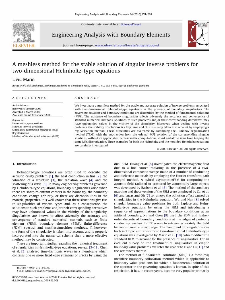
Fig. 5. Analytical and numerical solutions for (a) qjDO and (b) ujOA, obtained using the TRM, nS ¼ 0 and pq ¼ 1% noise added into the Neumann data qjGN, for Example 1.

x1

q


x1

u


x1

-1

0

1

2

3

1.0*10-6

1.0*10-5

1.0*10-4

1.0*10-3

1.0*10-2

1.0*10-1

1.0*100

Nor

mal

ized

err

or e

rr(q

(x))

nS = 1 nS = 2nS = 3 nS = 4nS = 5

x1

0.0

0.2

0.4

0.6

0.8

1.0*10-5

1.0*10-4

1.0*10-3

1.0*10-2

1.0*10-1

1.0*100

Nor

mal

ized

err

or e

rr(u

(x))

nS = 1 nS = 2nS = 3 nS = 4nS = 5

0.0 0.2 0.4 0.6 0.8 1.0

0.0 0.2 0.4 0.6 0.8 1.0-1.0 -0.8 -0.6 -0.4 -0.2 0.0

-1.0 -0.8 -0.6 -0.4 -0.2 0.0

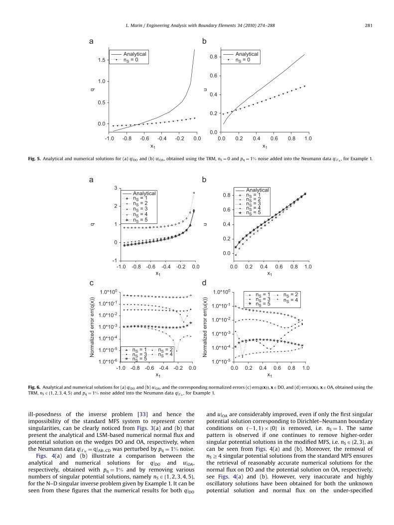
Fig. 6. Analytical and numerical solutions for (a) qjDO and (b) ujOA, and the corresponding normalized errors (c) errðqðxÞÞ, xADO, and (d) errðuðxÞÞ, xAOA, obtained using the

TRM, nS Af1;2;3;4;5g and pq ¼ 1% noise added into the Neumann data qjGN, for Example 1.


ill-posedness of the inverse problem [33] and hence theimpossibility of the standard MFS system to represent cornersingularities, can be clearly noticed from Figs. 3(a) and (b) thatpresent the analytical and LSM-based numerical normal flux andpotential solution on the wedges DO and OA, respectively, whenthe Neumann data qjGN

¼ qjAB[CD was perturbed by pq ¼ 1% noise.Figs. 4(a) and (b) illustrate a comparison between the

analytical and numerical solutions for qjDO and ujOA,respectively, obtained with pq ¼ 1% and by removing variousnumbers of singular potential solutions, namely nSAf1;2;3;4;5g,for the N–D singular inverse problem given by Example 1. It can beseen from these figures that the numerical results for both qjDO

and ujOA are considerably improved, even if only the first singularpotential solution corresponding to Dirichlet–Neumann boundaryconditions on ð�1;1Þ � f0g is removed, i.e. nS ¼ 1. The samepattern is observed if one continues to remove higher-ordersingular potential solutions in the modified MFS, i.e. nSAf2;3g, ascan be seen from Figs. 4(a) and (b). Moreover, the removal ofnSZ4 singular potential solutions from the standard MFS ensuresthe retrieval of reasonably accurate numerical solutions for thenormal flux on DO and the potential solution on OA, respectively,see Figs. 4(a) and (b). However, very inaccurate and highlyoscillatory solutions have been obtained for both the unknownpotential solution and normal flux on the under-specified

ARTICLE IN PRESS


boundary BC and these are presented in Figs. 4(c) and (d),respectively.

Although not presented, it is reported that similar results havebeen obtained for the other examples investigated in this study.Therefore, in order to retrieve accurate and stable numericalsolutions for singular inverse problem associated with Helmholtz-type equations, the use of the SST in the modified MFS approachonly is not sufficient, as clearly shown in Figs. 4(a)–(d).

7.4. Effect of the Tikhonov regularization

If solely the TRM is employed to solve the resulting MFSsystem (25) without removing any singular potential solutionsthen again very inaccurate numerical results have been retrievedfor both the potential solution and the normal flux. These resultsare presented in Figs. 5(a) and (b) which illustrate the analyticaland numerical normal flux and potential solution on the wedgesDO and OA, respectively, when qjGN

¼ qjAB[CD was perturbed bypq ¼ 1% noise and nS ¼ 0, in the case of Example 1. By comparingFigs. 3–5, we can conclude that both the SST and the TRM shouldbe employed in order to solve the singular inverse problem givenby Example 1 in a stable and accurate manner.

Indeed, if these two techniques are used together then thedifficulties caused by the ill-posedness of the inverse problem, aswell as the boundary singularity at O, can be overcome. Figs. 6(a)and (b) present the analytical and numerical results for the normal

10-10 10-5 100

Regularization parameter

1*10-3

1*10-2

1*10-1

1*100

1*101

RM

S e

rror

eu

(BC

)

pq = 1%pq = 3%pq = 5%

Residua

100

101

102

103

104

105

106

Sol

utio

n no

rm ||

c||

pq = 1%pq = 3%pq = 5%

0.02 0.04

Fig. 7. The RMS errors: (a) euðBCÞ, (b) eqðBCÞ, and (c) the corresponding L-curve, obtaine

qjGN, namely pq Af1%;3%;5%g, for Example 1.

flux on DO and potential solution on OA, respectively, retrieved bysolving the MFSþSST system of linear algebraic equations (25) usingthe TRM, in conjunction with the L-curve criterion for choosing theoptimal regularization parameter, pq ¼ 1% and nSAf1;2;3;4;5g, inthe case of Example 1. From these figures it can be noticed that theeffect of SST in the presence of the TRM is remarkable. When theTRM is employed then even the removal of the first two singularpotential solutions, i.e. nS ¼ 2, provides a very accurate numericalapproximation for the potential solution ujOA, which is also boundedand exempted from oscillations. Similar estimations are also valid forthe numerical normal flux qjDO, with the mention that, as expected,the numerical results obtained for the normal flux on DO are moreinaccurate than those retrieved for the potential solution on OA. Thesame conclusion can also be drawn from Figs. 6(c) and (d) whichpresent the results shown in Figs. 6(a) and (b) in terms of thenormalized errors errðqðxÞÞ, xADO, and errðuðxÞÞ, xAOA,respectively, as defined by formula (41). On comparing Figs. 3–6,we can conclude that the TRM provides very accurate MFSþSST-based numerical solutions to singular inverse problems forHelmholtz-type equations, at the same time having a regularizing/stabilizing effect on the MFSþSST solutions to such problems.

7.5. Choice of the optimal regularization parameter

Figs. 7(a) and (b) illustrate the relative RMS errors euðBCÞ andeqðBCÞ, respectively, given by relations (39) and (40), as functions

10-10 10-5 100

Regularization parameter

10-2

10-1

100

101

102

RM

S e

rror

eq

(BC

)

pq = 1%pq = 3%pq = 5%

l norm ||A c - F||0.07 0.1 0.2

d using the TRM, nS ¼ 5 and various levels of noise added into the Neumann data,

ARTICLE IN PRESS


of the regularization parameter l, obtained with nS ¼ 5 andvarious levels of noise added into the input normal flux data qjGN

,for the inverse problem given by Example 1. From these figures itcan be seen that both errors euðBCÞ and eqðBCÞ decrease as thelevel of noise pq added into the input Neumann data decreases forall regularization parameters l and euðBCÞoeqðBCÞ for allregularization parameters l and a fixed amount pq of noiseadded into the input normal flux data qjGN

, i.e. the numericalresults obtained for the normal flux are more inaccurate thanthose retrieved for the potential solution on the under-specifiedboundary BC. Fig. 7(c) shows on a log–log scale the L-curvesobtained for nS ¼ 5 and various levels of noise added into theinput normal flux data in the case of Example 1. By comparing this

Table 1The relative RMS errors, euðBCÞ and eqðBCÞ, and the values for the corresponding

optimal regularization parameter, lopt, obtained using the LSM and TRM, nS ¼ 5

and various levels of noise added into the normal flux qjGN, namely

pq Af1%;3%;5%g, for Example 1.

Method pq (%) eu ðBCÞ eq ðBCÞ lopt

LSM 1 0:33621� 101 0:78192� 102 –

3 0:10086� 102 0:23457� 103 –

5 0:16809� 102 0:39093� 103 –

TRM 1 0:51874� 10�2 0:10351� 10�1 1:0� 10�5

3 0:82568� 10�2 0:49427� 10�1 1:0� 10�5

5 0:11467� 10�1 0:90614� 10�1 1:0� 10�5

x1

q

Analyticalpq = 1%pq = 3%pq = 5%

x1

0.0

0.5

1.0

1.5

10-6

10-5

10-4

10-3

10-2

Nor

mal

ized

err

or e

rr(q

(x))

pq = 1%pq = 3%pq = 5%

-1.0 -0.8 -0.6 -0.4 -0.2 0.0

-1.0 -0.8 -0.6 -0.4 -0.2 0.0

Fig. 8. Analytical and numerical solutions for (a) qjDO and (b) ujOA, and the correspondin

TRM, nS ¼ 5 and various levels of noise added into the Neumann data, qjGN, namely pq

figure with Figs. 7(a) and (b), it can be seen, for various levels ofnoise, that the ‘‘corner’’ of the L-curve occurs at about the samevalue of the regularization parameter l where the minimum inthe accuracy errors euðBCÞ and eqðBCÞ is attained. Hence the choiceof the optimal regularization parameter lopt according to the L-curve criterion is fully justified. Similar results have been obtainedfor the Cauchy problems given by Examples 2 and 3 and thereforethey are not presented here.

Table 1 presents the values of the relative RMS errors euðBCÞand eqðBCÞ obtained by both methods, namely the LSM and theTRM, with nS ¼ 5 and various levels of noise added into the inputnormal flux data qjGN

, namely pqAf1%;3%;5%g, in the case ofExample 1, as well as the optimal values for the regularizationparameter l. By considering this table and Figs. 3–6, we canconclude that the use of regularization methods, in conjunctionwith the SST+MFS approach, is fully justified and provides bothstable and accurate numerical results not only on the edgessharing the singularity point, but also on the under-specifiedboundary BC.

7.6. Numerical stability of the method

In order to investigate the numerical stability of the proposedmodified MFS algorithm described in Section 5, in conjunctionwith the L-curve method of Hansen [38] for selecting the optimalvalue for the regularization parameter, l, in what follows weconsider the inverse problems given by Examples 1–3, the

x1

u


x1

0.0

0.2

0.4

0.6

0.8

10-4

10-4

10-4

Nor

mal

ized

err

or e

rr(u

(x))

pq = 1%pq = 3%pq = 5%

0.0 0.2 0.4 0.6 0.8 1.0

0.0 0.2 0.4 0.6 0.8 1.0

g normalized errors (c) errðqðxÞÞ, xADO, and (d) errðuðxÞÞ, xAOA, obtained using the

Af1%;3%;5%g, for Example 1.

ARTICLE IN PRESS

x1

u


x1

q


x1

0.0

0.5

1.0

10-5

10-5

10-4

10-4

10-3

10-3

10-2

Nor

mal

ized

err

or e

rr(u

(x))

pq = 1%pq = 3%pq = 5%

x1

0.0

0.1

0.2

0.3

0.4

10-5

10-4

10-3

10-2

10-1

Nor

mal

ized

err

or e

rr(q

(x))

pq = 1%pq = 3%pq = 5%

-1.0 -0.5 0.0 0.5 1.0

-1.0 -0.5 0.0 0.5 1.0

-1.0 -0.5 0.0 0.5 1.0

-1.0 -0.5 0.0 0.5 1.0

Fig. 9. Analytical and numerical solutions for (a) ujBC and (b) qjBC, and the corresponding normalized errors (c) errðuðxÞÞ, xABC, and (d) errðqðxÞÞ, xABC, obtained using the

TRM, nS ¼ 5 and various levels of noise added into the Neumann data, qjGN, namely pq Af1%;3%;5%g, for Example 1.

Table 2

The numerically retrieved values, aðnumÞj , for the flux intensity factors and the corresponding absolute errors, ErrðajÞ, obtained using the TRM , nS ¼ 5 and various levels of

noise added into the normal flux qjGN, namely pq Af1%;3%;5%g, for Example 1.

pq (%) aðnumÞ1

Errða1Þ aðnumÞ2

Errða2Þ aðnumÞ3

Errða3Þ aðnumÞ4

Errða4Þ

1 1.0027 0:27� 10�2 �1.3009 0:85� 10�3 1.5182 0:18� 10�1 �1.6997 0:29� 10�3

3 1.0031 0:31� 10�2 �1.2988 0:12� 10�2 1.5472 0:47� 10�1 �1.7833 0:83� 10�1

5 1.0036 0:36� 10�2 �1.2967 0:37� 10�2 1.5761 0:76� 10�1 �1.8670 0:17� 100


corresponding MFS discretizations mentioned in Section 7.1 andnS ¼ 5, whilst at the same time varying the level of noise addedinto the Dirichlet or Neumann data as pu; pqAf1%;3%;5%g.

Figs. 8(a) and (b) present the numerical normal flux on theboundary DO and potential solution on the boundary OA,respectively, obtained using the MFSþSST algorithm for variouslevels of Gaussian random noise added into the normal flux qjGN

,in the case of Example 1, in comparison with their analyticalvalues. From these figures it can be seen that, for all amounts, pq,of noise added into qjGN

, both the numerical potential solution onOA and the normal flux on DO represent excellent approximationsfor their analytical counterparts, being at the same time exemptedfrom high and unbounded oscillations in the vicinity of thesingularity. Similar conclusions can be drawn from Figs. 8(c) and(d) which show the normalized errors errðqðxÞÞ, xADO, and

errðuðxÞÞ, xAOA, respectively, associated with the numericalresults illustrated in Figs. 8(a) and (b). The numerical potentialsolution and normal flux on the under-specified boundary BC, aswell as their corresponding normalized errors, obtained using theregularized MFSþSST and pqAf1%;3%;5%g, are illustrated in Figs.9(a)–(d). From these figures we can conclude that the numericalresults for the potential solution and normal flux on the under-specified boundary BC are also in very good agreement with theircorresponding exact values and, in addition, they are convergentand stable with respect to decreasing the amount of noise addedinto the input boundary normal flux qjGN

. Accurate, stable andconvergent numerical results with respect to decreasing pq havealso been obtained for the flux intensity factors aj, j¼ 1; . . . ;4, andthese, together with their associated absolute errors ErrðajÞ,j¼ 1; . . . ;4, are presented in Table 2.

ARTICLE IN PRESS

x2

q

Analyticalpu = 1%pu = 3%pu = 5%

x1

q


x1

-0.6

-0.4

-0.2

0.0

0.2

3.5

3.55

3.6

3.65

3.7

3.75

3.8

u


x1

-0.75

-0.7

-0.65

-0.6

-0.55

0.4

0.5

0.6

0.7

0.8

0.9

q


0.0 0.2 0.4 0.6 0.8 1.0-1.0 -0.8 -0.6 -0.4 -0.2 0.0

-1.0 -0.5 0.0 0.5 1.0 -1.0 -0.5 0.0 0.5 1.0

Fig. 10. Analytical and numerical solutions for (a) qjEO, (b) qjOA, (c) ujBC, and (d) qjBC, obtained using the TRM, nS ¼ 5 and various levels of noise added into the Dirichlet

data, ujGD, namely pu Af1%;3%;5%g, for Example 2.

Table 3The relative RMS errors, euðBCÞ and eqðBCÞ, and the values for the corresponding

optimal regularization parameter, lopt, obtained using the LSM and TRM, nS ¼ 5

and various levels of noise added into the potential solution ujGD, namely

pu Af1%;3%;5%g, for Example 2.

Method pu (%) eu ðBCÞ eq ðBCÞ lopt

LSM 1 0:13585� 101 0:50453� 102 –

3 0:40755� 101 0:15136� 103 –

5 0:67924� 101 0:25226� 103 –

TRM 1 0:54359� 10�3 0:48179� 10�2 1:0� 10�4

3 0:91608� 10�3 0:54250� 10�2 1:0� 10�3

5 0:20574� 10�2 0:15029� 10�1 1:0� 10�3


The second example analysed in this paper is related again tothe modified Helmholtz equation and contains a singularity at theorigin O, which is caused by a sharp corner in the boundary, aswell as the nature of the analytical potential solution correspond-ing to this problem, see Eqs. (11) and (37), for perturbed boundarypotential measurements ujGD

. The analytical and numerical fluxeson the boundaries EO and OA obtained in this case are shown inFigs. 10(a) and (b), respectively. Although not presented, it isworth mentioning that the numerical flux obtained on EO [ OAusing the standard MFS ðnS ¼ 0Þ exhibits very high oscillations inthe neighbourhood of the singular point and hence it representsan inaccurate approximation for the analytical flux. The numericalpotential solution and normal flux on the under-specifiedboundary BC, obtained using the regularized MFSþSST forvarious levels of noise added into ujGD

, are illustrated inFigs. 10(c) and (d), respectively. The effect of the TRM and theMFSþSST algorithm on the accuracy of the numerical results incomparison with the LSM is clearly displayed in Table 3, whichpresents the relative RMS errors, euðBCÞ and eqðBCÞ, and the valuesfor the corresponding optimal regularization parameter, lopt,obtained on the under-specified boundary BC using the LSM andTRM. From Figs. 10(c) and (d) and Table 3 we can conclude that thenumerical results for the potential solution and normal flux on theunder-specified boundary BC are also excellent approximationsfor their corresponding exact values and, in addition, they areconvergent and stable with respect to decreasing the amount ofnoise added into the input boundary potential solution ujGD

.

Consider now the singular inverse problem for the two-dimensional Helmholtz equation, as given by Example 3, withperturbed boundary potential solution on GD. This singularCauchy problem is actually the most severe one among theinverse problems investigated in this study, in the sense that thesingularity at O is caused by all factors that may occur in such asituation, namely a sharp re-entrant corner and abrupt change inboundary conditions on the side DO [ OA (here ujOA and qjDO areprescribed), see Fig. 1(c), as well as the nature of the analyticalpotential solution corresponding to this problem, see Eqs. (12) and(38). Figs. 11(a) and (b) present the numerical solutions for the

ARTICLE IN PRESS

x1

u


x1

q

u q


x1

-0.3

-0.2

-0.1

0.0

0.1

-0.2

-0.1

0.0

0.1

0.2

0.3Analyticalpu = 1%pu = 3%pu = 5%

x1

-0.2

-0.15

-0.1

-0.05

0.2

0.22

0.24

0.26

0.28


0.0 0.2 0.4 0.6 0.8 1.0-1.0 -0.8 -0.6 -0.4 -0.2 0.0

-1.0 -0.5 0.0 0.5 1.0 -1.0 -0.5 0.0 0.5 1.0

Fig. 11. Analytical and numerical solutions for (a) ujDO and (b) qjOA, (c) ujBC, and (d) qjBC, obtained using the TRM, nS ¼ 5 and various levels of noise added into the

Dirichlet data, ujGD, namely pu Af1%;3%;5%g, for Example 3.

Table 4

The numerically retrieved values, aðnumÞj , for the flux intensity factors and the corresponding absolute errors, ErrðajÞ, obtained using the TRM, nS ¼ 5 and various levels of

noise added into the potential solution ujGD, namely pu Af1%;3%;5%g, for Example 3.

pu (%) aðnumÞ1

Errða1Þ aðnumÞ2

Errða2Þ aðnumÞ3

Errða3Þ aðnumÞ4

Errða4Þ

1 0.0048 0:48� 10�2 1.0142 0:14� 10�1 �1.5214 0:21� 10�1 1.0863 0:21� 100

3 0.0086 0:86� 10�2 1.0411 0:41� 10�1 �1.5404 0:40� 10�1 0.5801 0:72� 100

5 0.0116 0:12� 10�1 1.0463 0:46� 10�1 �1.5564 0:56� 10�1 0.4862 0:81� 100


potential solution ujDO and normal flux qjOA, respectively,retrieved by the TRM and various levels of noise added intoujGD

, in comparison with their analytical counterparts, forExample 3. It can be seen from these figures that the numericalresults for both the potential solution and the normal flux on theedges adjacent to the singularity point O are in very goodagreement with their corresponding analytical values and beingat the same time exempted from high and unbounded oscillations.Accurate, stable and convergent results have also been obtainedfor the unspecified potential solution ujBC and normal flux qjBC

when the modified MFS described in Section 5, as can be observedform Figs. 11(c) and (d), respectively. However, the numericalnormal fluxes qjBC are more inaccurate than the associatedpotential solutions ujBC, as can be noticed by comparingFigs. 11(c) and (d), and this is a direct consequence of the

severity of the singular inverse problem given by Example 3. Inaddition, from these figures it can be concluded that bothnumerical potential solutions and normal fluxes on the under-specified boundary BC are convergent and stable with respect todecreasing pu. Similar conclusions can be drawn from Table 4,which tabulates the numerical flux intensity factors, aðnumÞ

j ,j¼ 1; . . . ;4, and the corresponding absolute errors, ErrðajÞ,j¼ 1; . . . ;4, obtained using the TRM and various levels of noiseadded into the potential solution ujGD

.Overall, from the numerical results presented in this section it

can be concluded that the MFSþSST proposed in Section 5,combined with the TRM and Hansen’s L-curve criterion describedin Section 6, is a very suitable method for solving inverseboundary value problems exhibiting singularities caused by thepresence of sharp corners in the boundary of the solution domain

ARTICLE IN PRESS


and/or abrupt changes in the boundary conditions, for two-dimensional Helmholtz-type equations with noisy boundary data.The numerical potential solutions and normal fluxes retrievedusing this regularized MFSþSST are very good approximations fortheir analytical values on the entire boundary, they are exemptedfrom oscillations in the neighbourhood of the singularity pointand there is no need of further mesh refinement in the vicinity ofthe singularities.

8. Conclusions

In this study, the MFS was applied for solving, in an accu-rate and stable manner, inverse problems associated withtwo-dimensional Helmholtz-type equations in the presence ofboundary singularities. The existence of such boundary singula-rities affect adversely the accuracy and convergence of standardnumerical methods. Therefore, the MFS solutions to suchproblems and/or their corresponding derivatives, obtained by adirect inversion of the MFS system, may have unbounded valuesin the vicinity of the singularity. This difficulty was overcome bysubtracting from the original MFS solution the correspondingsingular potential solutions, as given by the asymptotic expansionof the potential solution near the singularity point, and at thesame time employing the TRM, in conjunction with Hansen’s L-curve method for choosing the optimal regularization parameter.Hence, in addition to the original MFS unknowns, new unknownswere introduced, namely the so-called flux intensity factors.Consequently, the original MFS system was extended by consider-ing a number of additional equations which equals the number offlux intensity factors introduced and specifically imposes the typeof singularity analysed in the vicinity of the singularity point. Theproposed MFSþSST was implemented and analysed for singularinverse problems associated with both the Helmholtz and themodified Helmholtz equations in two-dimensional domainscontaining an edge crack or a V-notch, as well as an L-shapeddomain.

From the numerical results presented in this paper, we canconclude that the advantages of the proposed method over othermethods, such as mesh refinement in the neighbourhood of thesingularity, the use of singular BEMs and/or FEMs etc., are the highaccuracy which can be obtained even when employing a smallnumber of collocation points and sources, and the simplicity ofthe computational scheme. A possible drawback of the presentmethod is the difficulty in extending the method to deal withsingularities in three-dimensional problems since such an exten-sion is not straightforward. The extension of the current approachto inverse boundary value problems associated with two-dimen-sional isotropic linear elastic materials, as well as two-dimen-sional biharmonic equation, is currently under investigation.

Acknowledgements

The financial support received from the Romanian Ministry ofEducation, Research and Innovation through IDEI Programme,Exploratory Research Projects, Grant PN II–ID–PCE–1248/2008, isgratefully acknowledged.

References

[1] Chen JT, Wong FC. Dual formulation of multiple reciprocity method for theacoustic mode of a cavity with a thin partition. Journal of Sound and Vibration1998;217:75–95.

[2] Kraus AD, Aziz A, Welty J. Extended surface heat transfer. New York: Wiley; 2001.[3] Chen JT, Liang MT, Chen IL, Chyuan SW, Chen KH. Dual boundary element

analysis of wave scattering from singularities. Wave Motion 1999;30:367–81.

[4] Huang C, Wu Z, Nevels RD. Edge diffraction in the vicinity of the tip of acomposite wedge. IEEE Transactions on Geoscience and Remote Sensing1993;31:1044–50.

[5] Barbone PA, Montgomery JM, Michael O, Harari I. Scattering by a hybridasymptotic/finite element. Computer Methods in Applied Mechanics andEngineering 1998;164:141–56.

[6] Cai W, Lee HC, Oh HS. Coupling of spectral methods and the p-version for thefinite element method for elliptic boundary value problems containingsingularities. Journal of Computational Physics 1993;108:314–26.

[7] Lucas TR, Oh HS. The method of auxiliary mapping for the finite elementsolutions of elliptic problems containing singularities. Journal of Computa-tional Physics 1993;108:327–42.

[8] Wu X, Han H. A finite-element method for Laplace- and Helmholtz-typeboundary value problems with singularities. SIAM Journal on NumericalAnalysis 1997;134:1037–50.

[9] Xu YS, Chen HM. Higher-order discretised boundary conditions at edges for TEwaves. IEEE Proceedings—Microwave Antennas and Propagation1999;146:342–8.

[10] Marin L, Lesnic D, Mantic V. Treatment of singularities in Helmholtz-typeequations using the boundary element method. Journal of Sound andVibration 2004;278:39–62.

[11] Li Z-C, Lu TT. Singularities and treatments of elliptic boundary valueproblems. Mathematical and Computer Modelling 2000;31:97–145.

[12] Mathon R, Johnston RL. The approximate solution of elliptic boundary valueproblems by fundamental solutions. SIAM Journal on Numerical Analysis1977;14:638–50.

[13] Fairweather G, Karageorghis A. The method of fundamental solutions forelliptic boundary value problems. Advances in Computational Mathematics1998;9:69–95.

[14] Golberg MA, Chen CS. The method of fundamental solutions for potential,Helmholtz and diffusion problems. In: Golberg MA, editor. Boundary integralmethods: numerical and mathematical aspects. Boston: WIT Press andComputational Mechanics Publications; 1999. p. 105–76.

[15] Fairweather G, Karageorghis A, Martin PA. The method of fundamentalsolutions for scattering and radiation problems. Engineering Analysis withBoundary Elements 2003;27:759–69.

[16] Cho HA, Golberg MA, Muleshkov AS, Li X. Trefftz methods for time dependentpartial differential equations. CMC: Computers, Materials & Continua2004;1:1–37.

[17] Hon YC, Wei T. A fundamental solution method for inverse heat conductionproblems. Engineering Analysis with Boundary Elements 2004;28:489–95.

[18] Mera NS. The method of fundamental solutions for the backward heatconduction problem. Inverse Problems in Science and Engineering2005;13:79–98.

[19] Marin L, Lesnic D. The method of fundamental solutions for the Cauchyproblem in two-dimensional linear elasticity. International Journal of Solidsand Structures 2004;41:3425–38.

[20] Marin L. A meshless method for solving the Cauchy problem in three-dimensional elastostatics. Computers & Mathematics with Applications2005;50:73–92.

[21] Marin L. Numerical solutions of the Cauchy problem for steady-state heattransfer in two-dimensional functionally graded materials. InternationalJournal of Solids and Structures 2005;42:4338–51.

[22] Marin L, Lesnic D. The method of fundamental solutions for the Cauchyproblem associated with two-dimensional Helmholtz-type equations. Com-puters & Structures 2005;83:267–78.

[23] Marin L. A meshless method for the numerical solution of the Cauchyproblem associated with three-dimensional Helmholtz-type equations.Applied Mathematics and Computation 2005;165:355–74.

[24] Jin B, Zheng Y. A meshless method for some inverse problems associated withthe Helmholtz equation. Computer Methods in Applied Mechanics andEngineering 2006;195:2270–80.

[25] Jin B, Marin L. The method of fundamental solutions for inverse sourceproblems associated with the steady-state heat conduction. InternationalJournal for Numerical Methods in Engineering 2007;69:1570–89.

[26] Karageorghis A. Modified methods of fundamental solutions for harmonicand biharmonic problems with boundary singularities. Numerical Methodsfor Partial Differential Equations 1992;8:1–19.

[27] Poullikkas A, Karageorghis A, Georgiou G. Methods of fundamental solutionsfor harmonic and biharmonic boundary value problems. ComputationalMechanics 1998;21:416–23.

[28] Karageorghis A, Poullikkas A, Berger JR. Stress intensity factor computationusing the method of fundamental solutions. Computational Mechanics2006;37:445–54.

[29] Berger JR, Karageorghis A, Martin PA. Stress intensity factor computationusing the method of fundamental solutions: mixed mode problems.International Journal for Numerical Methods in Engineering 2007;69:469–83.

[30] Marin L. Stable MFS solution to singular direct and inverse problemsassociated with the Laplace equation subjected to noisy data. CMES:Computer Modeling in Engineering & Sciences 2008;37:203–42.

[31] Marin L. Treatment of singularities in the method of fundamental solutionsfor two-dimensional Helmholtz-type equations. Applied MathematicalModelling, 2009 [in press], doi:10.1016/j.apm.2009.09.009.

[32] Portela A, Aliabadi MH, Rooke DP. Dual boundary element analysis of crackedplates: singularity subtraction technique. International Journal Fracture1992;55:17–28.

10.1016/j.apm.2009.09.009

ARTICLE IN PRESS


[33] Hadamard J. Lectures on Cauchy problem in linear partial differentialequations. New Haven: Yale University Press; 1923.

[34] Gorzelanczyk P, Ko"odziej A. Some remarks concerning the shape of the shapecontour with application of the method of fundamental solutions to elastictorsion of prismatic rods. Engineering Analysis with Boundary Elements2008;32:64–75.

[35] Tikhonov AN, Arsenin VY. Methods for solving ill-posed problems. Moscow:Nauka; 1986.

[36] Morozov VA. On the solution of functional equations by the method ofregularization. Soviet Mathematical Doklady 1966;7:414–7.

[37] Wahba G. Practical approximate solutions to linear operator equations whenthe data are noisy. SIAM Journal on Numerical Analysis 1977;14:651–67.

[38] Hansen PC. Rank-deficient and discrete ill-posed problems: numericalaspects of linear inversion. Philadelphia: SIAM; 1998.

a meshless method for the stable solution of singular inverse problems for two-dimensional...

Documents