a measurement of the proton-proton inelastic scattering ... · a measurement of the proton-proton...
TRANSCRIPT

CER
N-T
HES
IS-2
011-
046
13/0
5/20
11
A Measurement of the proton-proton inelastic scattering cross-section at√s = 7 TeV with
the ATLAS detector at the LHC
by
Lauren Alexandra Tompkins
A dissertation submitted in partial satisfaction of the
requirements for the degree of
Doctor of Philosophy
in
Physics
in the
Graduate Division
of the
University of California, Berkeley
Committee in charge:
Professor B. H. Heinemann, Chair
Professor Y. Kolomensky
Professor L. Blitz
Spring 2011

A Measurement of the proton-proton inelastic scattering cross-section at√s = 7 TeV with
the ATLAS detector at the LHC
Copyright 2011
by
Lauren Alexandra Tompkins

1
Abstract
A Measurement of the proton-proton inelastic scattering cross-section at√s = 7 TeV with
the ATLAS detector at the LHC
by
Lauren Alexandra Tompkins
Doctor of Philosophy in Physics
University of California, Berkeley
Professor B. H. Heinemann, Chair
The first measurement of the inelastic cross-section for proton-proton collisions at a center
of mass energy√s = 7 TeV using the ATLAS detector at the Large Hadron Collider is
presented. From a dataset corresponding to an integrated luminosity of 20 µb−1, events are
selected by requiring activity in scintillation counters mounted in the forward region of the
ATLAS detector. An inelastic cross-section of 60.1 ± 2.1 mb is measured for the subset
of events visible to the scintillation counters. The uncertainty includes the statistical and
systematic uncertainty on the measurement. The visible events satisfy ξ > 5×10⁻⁶, where
ξ = M2X/s is calculated from the invariant mass, MX , of hadrons selected using the largest
rapidity gap in the event. For diffractive events this corresponds to requiring at least one
of the dissociation masses to be larger than 15.7 GeV. Using an extrapolation dependent
on the model for the differential diffractive mass distribution, an inelastic cross-section
of 69.1 ± 2.4(exp) ± 6.9(extr) mb is determined, where (exp) indicates the experimental
uncertainties and (extr) indicates the uncertainty due to the extrapolation from the limited
ξ-range to the full inelastic cross-section.

i
To Dad,
for the tool bench,
and Mom,
for the secrets of math and broccoli.

ii
ACKNOWLEDGMENTS
When I first joined the LBL ATLAS group as a wide-eyed young graduate student, I
never dreamed that my dissertation research would involve measuring the inelastic proton-
proton cross-section. Five years and one massive accelerator accident later, I feel fortunate
to have been given an opportunity to own an LHC analysis in a way that would not have
been possible with almost any other topic. I owe that opportunity to my adviser, Beate
Heinemann. Throughout the past year she has been the trench commander on the front
lines of this analysis with me. I have learned so much from her in this work and in the
wide variety of other topics we have covered over the past four years. Along the way I
have developed a deep respect and admiration for the way she does physics and the way
she works with other people.
While Beate has been my primary mentor, I have also received much support and wis-
dom from past and present members of the LBL ATLAS group. This formidable group
of physicists has given me better training than I could have gotten anywhere else. A few
people deserve specific mention. Sven Vahsen was my guide when writing my first Athena
code, and he taught me much during the cosmics analysis. Marjorie Shapiro has always
been a willing mentor, providing valuable insight on whatever project I was working on.
My dissertation is a small part of the work done by the ATLAS Soft QCD group. Analyzing
the first LHC data was exciting, but the Min-Bias folks, who dove into the data with relish
on day one, made it fun as well. The cross-section analysis was greatly improved by the
guidance of its Editorial Board. In particular, the expertise of Emily Nurse, Paul Newman,
and Halina Abramowicz, and the stewardship of Jon Butterworth and Kevin Einsweiller
was crucial for navigating the muddled waters of soft interactions.
My work on ATLAS began in 2004 with the Orsay group in France. My thanks go to
Daniel Fournier for sponsoring me as a completely unknown American student, Laurent
Serin for giving me my first hardware experience, and Dirk Zerwas for advising me on my
first full analysis. I would also like to thank my undergraduate adviser, Young-Kee Kim.
Her dedication, enthusiasm and support made research an exciting and wonderful thing.
My higher education journey has encompassed much more than learning to do a physics
analysis. Over a third of my life has been spent in the arms of the University of California,
to which I am greatly indebted. No place has ever felt more like home. I owe a big thank-
you to my friends from the cohort of 2005 and the wonderful people with whom they share

iii
their lives. The ski weekends and Wednesday night dinners were a welcome respite from
work. I have to thank Heather, without whom I would’ve never survived my stay at CERN.
Max has been my solid, and oftentimes vocal, companion during the ups and downs of
being an LHC grad student. I am so thankful to have spent the past few years sharing an
office and a friendship with him.
My long friendship with Dana, Jasmin and Vidya has sustained me through the chal-
lenges of freshman problem sets and mid-twenties angst alike. Each of them is an inspi-
ration in ways that I could never enumerate. My deepest thanks goes to Mom, Dad, Katie
and Sean: I am who I am and where I am because of your love and encouragement. And
lastly I want to thank Kyle. Through him I have learned what is truly important in life.
Funding for my work was provided by the American Taxpayer, in the guise of a Na-
tional Science Foundation Graduate Fellowship (2005-2008) and funds from the US De-
partment of Energy. I am honored to be supported in doing what I love.

iv
PREFACE
For the General Reader
On March 30th, 2010, the highest-energy man-made proton collisions to date occurred
at the Large Hadron Collider (LHC) in Geneva, Switzerland, ushering in a new era of
discovery for high-energy particle physics. The LHC is poised to answer some of the most
fundamental questions of nature: what is the origin of mass? is our current understanding
of elementary particle interactions a complete description of nature? and, possibly, what
is the nature of dark matter? The work in this thesis concerns the first steps along the
road to discovery. It aims for an understanding of the most abundant and inclusive of LHC
processes, proton-proton inelastic collisions.
The LHC is a proton collision factory, churning out millions of collisions per second. It
takes hydrogen atoms from a tank of gas, strips the atoms of their electrons, and accelerates
the remaining protons to 99.999996% of the speed of light. The protons revolve around the
LHC in two beams traveling in opposite directions, and are brought to collide at four points
along the 27 km ring in a region no larger than a strand of hair. Each beam is divided into
multiple bunches of 100 billion protons to maximize the probability that the protons will
interact when the beams cross each other; even at those beam densities, only a few proton
interactions occur per beam crossing.
Garden-variety proton-proton interactions happen 10 billion times more frequently than
theorists predict interactions which produce the fabled Higgs boson should occur. Yet,
the theorists cannot calculate from first principles how often protons interact with each
other. By contrast, they can predict with relatively high accuracy how often a proton-
proton interaction will yield a Higgs Boson. The reason that the rare Higgs production rate
is easier to calculate than the total proton-proton interaction rate is because of what inside
the proton is interacting. To produce a Higgs boson, which is a heavy particle, a large
amount of energy is needed so very energetic parts of the proton must interact. However,
only a small part of the proton carries significant energy, the rest is a teeming, low energy
mess.Think of the proton as a ball of jello with a few BBs embedded inside of it. Most of

v
the time when two protons collide the jello makes a mess, but the BBs don’t contact each
other. However, on rare occasions a BB from one proton will hit one from the other proton
head on and the result with be a clean interaction, like the collision of two billiard balls.
Calculating the interaction of jello with jello is intractable, but calculating the interaction
of two BBs is simple. Higgs boson production occurs in the rare “BB” collisions, the vast
majority of LHC collisions, such as the one shown in Figure 1, are made of “jello”.
Figure. 1 A proton-proton collision event from the first day of 7 TeV collisions at the LHC. The outermost
blue segments indicate the muon detectors. The pink and green regions indicate the hadronic and electromag-
netic calorimeters, respectively. The grey shaded region shows the inner tracking detectors. The colored lines
are the traces of charged particles, as determined from the energy deposits left in the detector by the particle,
indicated by the grey dots. The left view is transverse to the beam direction, the upper right view is along the
beam direction.
One of the most interesting features of proton-proton interactions is how the rate of
interaction changes with different proton collision energies. How quickly the interaction
rate increases sheds light on what mechanisms are involved in the interactions at different
energies. Because the rate of proton interactions is so difficult to calculate, experimental
measurements are critical to distinguishing which models of the interactions best describe
nature. Measurements at past colliders mapped out the dependence of the interaction rate
at low proton energies and found a slow dependence on the energy. Once data were taken
at higher energies, the situation got murkier. For example, two experiments at the Fermilab
accelerator in Batavia, Illinois, which has proton energies three and a half times lower than
at the LHC, yielded discrepant results. At very high energies, cosmic ray data have been
used to infer the proton-proton interaction rate. When cosmic ray protons bombard the

vi
upper atmosphere they interact with atoms in the air. These interactions are measured by
experiments, and are related to proton-proton interactions through approximate theoretical
models. However, because these measurement rely on models and approximations, they
have large uncertainties. Therefore, they provide little information on the high energy
behavior of proton-proton interactions.
The measurement presented in this thesis uses the ATLAS detector at the LHC to mea-
sure the rate of proton-proton interactions at the highest energy man-made collisions in the
world. Events are detected and counted using scintillator discs which sit 3.6 m from the
center of ATLAS and have an inner radius of 14 cm and an outer radius of 88 cm from
beam-pipe. The scintillators are made of a special plastic which emits light when traversed
by a charged particle. The light signals that a proton-proton interaction has occurred.
beam-line
pp
Particle furthest
from beam-line
Scintillator Detectors
(a)
beam-line
pp
Particle furthest
from beam-line
Scintillator Detectors
(b)
Figure. 2 Cartoon sketch of an event illustrating which events are visible to the detector. The yellow discs
indicate the scintillator detectors, the red and blue dashed arrows represent particles created in a proton-proton
interaction. In Figure (a) the event is detected because the particles intersect the scintillators. In Figure (b) it
is not detected.
What distinguishes this measurement from measurements in the past is that it is re-
stricted to only the subset of proton-proton interactions which the detector can observe.
Most proton-proton interactions look like Figure 1. They are easily detectable because par-
ticles are produced in all directions. However, in some interactions the protons exchange

vii
only a bit of energy and the new particles created in the interaction are emitted at small
angles to the beam-line. Sometimes the new particles are so close to the beam-line that
the detector cannot measure them. Figure 2 illustrates two events. In Figure P.2a the par-
ticles produced intersect the scintillator detectors and the event is observed. In Figure P2b
the particles are too close to the beam-line and do not traverse the scintillators. Normally
experiments use models of how often this happens to correct for these undetected events.
The measurement in this thesis is defined as the rate of proton interactions in which the
particle furthest from the beam line intersects the innermost edge of the detector. Therefore
there is no large model-dependent correction for the undetected events. Because it is so
well-defined, the measurement has very small uncertainties. In order to compare with past
experiments and other models, this thesis also presents the interaction rate with a model-
dependent correction for the undetected events.
The measurement presented in this thesis is highest energy direct measurement of the
proton-proton interaction rate. The measurement does not show a dramatic rise of the
interaction rate at LHC energies, indicating that no new mechanism is involved in the
proton-proton interactions. Some models predict that at higher energies protons will inter-
act through new channels not present at lower energies and that these additional channels
will increase the interaction rate. The data suggest that this hypothesis is incorrect.

viii
Contents
List of Figures xi
List of Tables xiv
1 Introduction 1
2 pp Interactions: Models and Monte Carlo Models 4
2.1 Overview and Historical Development . . . . . . . . . . . . . . . . . . . . 4
2.2 Regge Theory and Pomeron Trajectories . . . . . . . . . . . . . . . . . . . 5
2.3 QCD and the Parton Model . . . . . . . . . . . . . . . . . . . . . . . . . . 9
2.4 Partonic Descriptions of the Pomeron . . . . . . . . . . . . . . . . . . . . 11
2.5 Analytic Cross-Section Models . . . . . . . . . . . . . . . . . . . . . . . . 13
2.5.1 Total Cross-Sections . . . . . . . . . . . . . . . . . . . . . . . . . 13
2.5.2 Inelastic and Diffractive Cross-sections . . . . . . . . . . . . . . . 16
2.6 Monte Carlo Models . . . . . . . . . . . . . . . . . . . . . . . . . . . . . 19
3 Inelastic Cross-Section Measurement Overview 26
4 The Large Hadron Collider 31
4.1 Motivation . . . . . . . . . . . . . . . . . . . . . . . . . . . . . . . . . . . 31
4.2 Design . . . . . . . . . . . . . . . . . . . . . . . . . . . . . . . . . . . . . 32
4.2.1 Accelerator Chain . . . . . . . . . . . . . . . . . . . . . . . . . . 32
4.2.2 Magnets . . . . . . . . . . . . . . . . . . . . . . . . . . . . . . . . 33
4.2.3 The September 19th Incident . . . . . . . . . . . . . . . . . . . . . 35
4.3 2010 Run Conditions . . . . . . . . . . . . . . . . . . . . . . . . . . . . . 35
5 The ATLAS Detector 37
5.1 Trigger and Data-Acquisition System . . . . . . . . . . . . . . . . . . . . 37
5.2 The Inner Detector . . . . . . . . . . . . . . . . . . . . . . . . . . . . . . 39
5.2.1 Pixel Detector . . . . . . . . . . . . . . . . . . . . . . . . . . . . . 40
5.2.2 Semi Conductor Tracker . . . . . . . . . . . . . . . . . . . . . . . 41
5.2.3 Transition Radiation Tracker . . . . . . . . . . . . . . . . . . . . . 42
5.3 The Calorimeters . . . . . . . . . . . . . . . . . . . . . . . . . . . . . . . 44

CONTENTS ix
5.3.1 Liquid Argon Electromagnetic Calorimeters . . . . . . . . . . . . . 44
5.3.2 The Tile Hadronic Calorimeter . . . . . . . . . . . . . . . . . . . . 46
5.3.3 Forward Calorimeters . . . . . . . . . . . . . . . . . . . . . . . . 47
5.4 The Muon Spectrometer . . . . . . . . . . . . . . . . . . . . . . . . . . . 48
5.5 The Luminosity Detectors . . . . . . . . . . . . . . . . . . . . . . . . . . 50
5.5.1 Minimum Bias Trigger Scintillators . . . . . . . . . . . . . . . . . 50
5.5.2 LUCID . . . . . . . . . . . . . . . . . . . . . . . . . . . . . . . . 50
6 Event Reconstruction 53
6.1 Track Reconstruction . . . . . . . . . . . . . . . . . . . . . . . . . . . . . 53
6.1.1 Reconstruction Algorithms . . . . . . . . . . . . . . . . . . . . . . 53
6.1.2 Tracking Efficiency . . . . . . . . . . . . . . . . . . . . . . . . . . 58
6.1.3 Track Resolution . . . . . . . . . . . . . . . . . . . . . . . . . . . 65
6.2 MBTS And Calorimeter Signal Reconstruction . . . . . . . . . . . . . . . 66
6.2.1 Liquid Argon Calorimeters . . . . . . . . . . . . . . . . . . . . . . 68
6.2.2 Tile Calorimeter and the MBTS . . . . . . . . . . . . . . . . . . . 68
7 Collision and Monte Carlo Datasets 71
7.1 Data . . . . . . . . . . . . . . . . . . . . . . . . . . . . . . . . . . . . . . 71
7.2 Monte Carlo Models . . . . . . . . . . . . . . . . . . . . . . . . . . . . . 72
8 MBTS Detector Response and Efficiency Measurements 74
8.1 Noise Profiles . . . . . . . . . . . . . . . . . . . . . . . . . . . . . . . . . 74
8.2 Trigger Efficiency . . . . . . . . . . . . . . . . . . . . . . . . . . . . . . . 76
8.3 Offline Efficiency Studies . . . . . . . . . . . . . . . . . . . . . . . . . . . 77
8.3.1 Efficiency Measurement with Tracks . . . . . . . . . . . . . . . . . 78
8.3.2 Efficiency Measurement with the Calorimeters . . . . . . . . . . . 80
8.4 Material . . . . . . . . . . . . . . . . . . . . . . . . . . . . . . . . . . . . 82
9 Backgrounds 89
9.1 Beam-Related Backgrounds . . . . . . . . . . . . . . . . . . . . . . . . . 89
9.1.1 Beam-Gas, Beam-Halo, Out-of-time Afterglow . . . . . . . . . . . 89
9.1.2 In-time Afterglow . . . . . . . . . . . . . . . . . . . . . . . . . . 92
9.2 Other Backgrounds . . . . . . . . . . . . . . . . . . . . . . . . . . . . . . 92
10 Luminosity Determination 94
10.1 Introduction to Luminosity and Beam Separation Scans . . . . . . . . . . . 94
10.2 Charged Particle Event Counting and Other Methods . . . . . . . . . . . . 96
10.2.1 Luminosity Detectors . . . . . . . . . . . . . . . . . . . . . . . . . 97
10.2.2 Luminosity Algorithms . . . . . . . . . . . . . . . . . . . . . . . . 97
10.2.3 Charged Particle Event Counting . . . . . . . . . . . . . . . . . . . 98
10.3 Beam Separation Scan Analysis . . . . . . . . . . . . . . . . . . . . . . . 101

CONTENTS x
10.3.1 Scan Descriptions . . . . . . . . . . . . . . . . . . . . . . . . . . . 101
10.3.2 Fits for Beam Parameters . . . . . . . . . . . . . . . . . . . . . . . 103
10.3.3 Uncertainties . . . . . . . . . . . . . . . . . . . . . . . . . . . . . 104
10.3.4 Results . . . . . . . . . . . . . . . . . . . . . . . . . . . . . . . . 108
11 Comparisons of Monte Carlo Modeling of Diffractive Events 111
11.1 Track-based Studies . . . . . . . . . . . . . . . . . . . . . . . . . . . . . . 111
11.1.1 Overview of Studies . . . . . . . . . . . . . . . . . . . . . . . . . 112
11.1.2 Datasets and Event Selection . . . . . . . . . . . . . . . . . . . . . 113
11.1.3 Acceptance . . . . . . . . . . . . . . . . . . . . . . . . . . . . . . 114
11.1.4 Data and Simulation Response Agreement . . . . . . . . . . . . . . 115
11.1.5 Systematic Uncertainties . . . . . . . . . . . . . . . . . . . . . . . 116
11.1.6 Comparisons . . . . . . . . . . . . . . . . . . . . . . . . . . . . . 118
11.2 MBTS Multiplicity-based Studies . . . . . . . . . . . . . . . . . . . . . . 120
11.3 Summary . . . . . . . . . . . . . . . . . . . . . . . . . . . . . . . . . . . 124
12 Results 128
12.1 Background Estimation . . . . . . . . . . . . . . . . . . . . . . . . . . . . 128
12.2 Acceptance . . . . . . . . . . . . . . . . . . . . . . . . . . . . . . . . . . 131
12.2.1 MBTS Acceptance . . . . . . . . . . . . . . . . . . . . . . . . . . 131
12.2.2 Fractional Contribution of Diffractive Processes . . . . . . . . . . . 134
12.2.3 ǫsel and fξ<5×10⁻⁶ . . . . . . . . . . . . . . . . . . . . . . . . . . . 135
12.2.4 Extrapolating to ξ > m2p/s . . . . . . . . . . . . . . . . . . . . . . 135
12.3 Systematic Uncertainties . . . . . . . . . . . . . . . . . . . . . . . . . . . 138
12.4 The Cross-section Measurement . . . . . . . . . . . . . . . . . . . . . . . 141
13 Conclusion 146
Bibliography 148
A Mandelstam Variables 157
B The Optical Theorem 159

xi
List of Figures
1.1 Proton-proton and proton-antiproton total cross-section data. . . . . . . . . 2
2.1 Proton-proton interactions. . . . . . . . . . . . . . . . . . . . . . . . . . . 6
2.2 Chew-Frautschi plot. . . . . . . . . . . . . . . . . . . . . . . . . . . . . . 7
2.3 pp and pp elastic scattering data. . . . . . . . . . . . . . . . . . . . . . . . 8
2.4 Feynman diagram of deep inelastic scattering. . . . . . . . . . . . . . . . . 10
2.5 Feynman diagram of two gluon exchange. . . . . . . . . . . . . . . . . . . 11
2.6 Illustration of p+ e→ e+X + p. . . . . . . . . . . . . . . . . . . . . . . 12
2.7 Proton-proton and proton-antiproton total cross-section data and fits. . . . . 15
2.8 Proton-proton and proton-antiproton inelastic cross-section data and fits. . . 17
2.9 ξ distribution for SD (left) and DD (right) events. . . . . . . . . . . . . . . 20
2.10 Diagram of single diffractive dissociation. . . . . . . . . . . . . . . . . . . 22
2.11 Multiplicity distributions for the MC generators. . . . . . . . . . . . . . . . 23
2.12 η distributions for the MC generators. . . . . . . . . . . . . . . . . . . . . 24
2.13 pT distributions for the MC generators. . . . . . . . . . . . . . . . . . . . . 25
3.1 Toy figure of diffractive events. . . . . . . . . . . . . . . . . . . . . . . . . 28
3.2 ξ distribution for MC generators. . . . . . . . . . . . . . . . . . . . . . . . 28
3.3 ξ versus min η. . . . . . . . . . . . . . . . . . . . . . . . . . . . . . . . . 29
4.1 The CERN accelerator complex. . . . . . . . . . . . . . . . . . . . . . . . 33
4.2 A cross section of the LHC dipole illustrating the twin-bore design. . . . . 34
4.3 Peak luminosity by day and integrated luminosity by day in 2010. . . . . . 36
5.1 A diagram of the ATLAS detector. . . . . . . . . . . . . . . . . . . . . . . 38
5.2 Cutaway of the ATLAS Inner Detector. . . . . . . . . . . . . . . . . . . . . 40
5.3 An r − z view of a quarter of the Inner Detector. . . . . . . . . . . . . . . 42
5.4 Material distributions at the exit of the ATLAS Inner Detector. . . . . . . . 43
5.5 Pixel and SCT barrel modules. . . . . . . . . . . . . . . . . . . . . . . . . 44
5.6 A TRT barrel module. . . . . . . . . . . . . . . . . . . . . . . . . . . . . . 45
5.7 A diagram of an electromagnetic calorimeter segment. . . . . . . . . . . . 46
5.8 A diagram of a tile drawer. . . . . . . . . . . . . . . . . . . . . . . . . . . 47
5.9 Forward Calorimeters. . . . . . . . . . . . . . . . . . . . . . . . . . . . . 48

LIST OF FIGURES xii
5.10 The ATLAS muon system. . . . . . . . . . . . . . . . . . . . . . . . . . . 49
5.11 MBTS design. . . . . . . . . . . . . . . . . . . . . . . . . . . . . . . . . . 51
5.12 The LUCID detector. . . . . . . . . . . . . . . . . . . . . . . . . . . . . . 52
6.1 An illustration of track parameters in the transverse and longitudinal planes. 54
6.2 Schematic of the different stages of track reconstruction. . . . . . . . . . . 56
6.3 Tracking efficiency as a function of η and pT. . . . . . . . . . . . . . . . . 59
6.4 Average number of pixel and SCT as a function of η. . . . . . . . . . . . . 60
6.5 δφ between Standalone TRT track and closest Silicon track. . . . . . . . . . 62
6.6 Relative efficiency of the Silicon tracking as a function of the pT. . . . . . . 63
6.7 Relative efficiency of the Silicon tracking as a function of for d0 and NTRT. 63
6.8 Toy example of half-tracks. . . . . . . . . . . . . . . . . . . . . . . . . . . 66
6.9 Track parameter resolutions and bias measured in cosmic ray data. . . . . . 67
6.10 Toy representation of a PMT pulse. . . . . . . . . . . . . . . . . . . . . . . 69
6.11 Difference in MBTS detector timing measurements on the A- and C-side. . 70
6.12 Liquid argon and tile calorimeter signal pulses. . . . . . . . . . . . . . . . 70
7.1 The material distribution in radiation lengths for different geometries. . . . 73
8.1 MBTS Noise distributions. . . . . . . . . . . . . . . . . . . . . . . . . . . 75
8.2 L MBTS 1 trigger efficiency. . . . . . . . . . . . . . . . . . . . . . . . . . 76
8.3 Track-based L1 MBTS 1 trigger efficiency. . . . . . . . . . . . . . . . . . 77
8.4 Track-tagged MBTS counter charge distributions. . . . . . . . . . . . . . . 78
8.5 Track-based fsig, fzero, and ǫ for MBTS Counters. . . . . . . . . . . . . . . 84
8.6 Detailed track-based fsig and ǫ for MBTS Counters. . . . . . . . . . . . . . 85
8.7 FCAL- and EMEC-tagged MBTS charge distributions. . . . . . . . . . . . 86
8.8 FCAL-based fsig, fzero, and ǫ for MBTS Counters. . . . . . . . . . . . . . . 87
8.9 EMEC-based fsig, fzero, and ǫ for MBTS Counters. . . . . . . . . . . . . . 88
9.1 Beam-gas vertex distributions. . . . . . . . . . . . . . . . . . . . . . . . . 90
9.2 L1 MBTS C trigger rate as a function of BCID. . . . . . . . . . . . . . . . 91
9.3 MBTS hit time distributions. . . . . . . . . . . . . . . . . . . . . . . . . . 93
10.1 Track to particle correction closure test. . . . . . . . . . . . . . . . . . . . 100
10.2 Rate of charged particle events in Fill 1089. . . . . . . . . . . . . . . . . . 101
10.3 Horizontal beam displacement in scansI-III. . . . . . . . . . . . . . . . . . 103
10.4 Rate of events with at least one track for scans I-III. . . . . . . . . . . . . . 103
10.5 Fit Results for vdM scans I-III. . . . . . . . . . . . . . . . . . . . . . . . . 109
10.6 Fit results for scan IV. . . . . . . . . . . . . . . . . . . . . . . . . . . . . . 110
11.1 Data to MC simulation comparison of track parameters. . . . . . . . . . . . 115
11.2 Data to MC simulation comparison of hits on track. . . . . . . . . . . . . . 116
11.3 1Nev
dNtrk
dηand 1
Nev
dNev
dntrkfor the single-sided selection. . . . . . . . . . . . . . 119
LIST OF FIGURES xiii
11.4 1Nev
12πpT
d2Ntrk
dηdpTfor the single-sided selection. . . . . . . . . . . . . . . . . 120
11.5 1/NevdNev/d∆η for the single-sided selection. . . . . . . . . . . . . . . . 121
11.6 1Nev
dntrk
dηfor each generator by sub-process. . . . . . . . . . . . . . . . . . 122
11.7 1Nev
dNev
dntrkfor each generator by sub-process. . . . . . . . . . . . . . . . . . 123
11.8 1Nev
12πpT
d2ntrk
dηdpTfor each generator by sub-process. . . . . . . . . . . . . . . 124
11.9 1Nev
dntrk
d∆ηfor each generator by sub-process. . . . . . . . . . . . . . . . . . 125
11.10MBTS inclusive multiplicity histograms. . . . . . . . . . . . . . . . . . . . 126
11.11MBTS single-sided multiplicity histograms. . . . . . . . . . . . . . . . . . 127
12.1 Efficiency of MBTS event selection as a function of ξ. . . . . . . . . . . . 133
12.2 Efficiency of the single-sided selection. . . . . . . . . . . . . . . . . . . . 134
12.3 RSS versus fD . . . . . . . . . . . . . . . . . . . . . . . . . . . . . . . . . 138
12.4 RSS versus fD with σDD
σSD= 1 and σDD
σSD= 0. . . . . . . . . . . . . . . . . . . 140
12.5 σinel(ξ > 5 × 10⁻⁶) and σinel versus√s including the Atlas measurement. . 145
A.1 Mandelstam variables. . . . . . . . . . . . . . . . . . . . . . . . . . . . . 158
B.1 An illustration of the optical theorem. . . . . . . . . . . . . . . . . . . . . 160

xiv
List of Tables
2.1 Cross sections for PYTHIA and for PHOJET at√s = 7 TeV. . . . . . . . . . 21
4.1 Comparison of the LHC machine conditions. . . . . . . . . . . . . . . . . 36
5.1 Summary of the dimensions of the Inner Detector subdetectors. . . . . . . . 41
6.1 Summary of relative silicon efficiencies uncertainties. . . . . . . . . . . . . 64
7.1 Summary of the data used in this analysis. . . . . . . . . . . . . . . . . . . 71
7.2 Summary of models used in the analysis. . . . . . . . . . . . . . . . . . . . 73
8.1 fsig, fzero, ǫ for track-tagged counters. . . . . . . . . . . . . . . . . . . . . 80
8.2 FCAL-tagged MBTS fsig, fzero, and ǫ. . . . . . . . . . . . . . . . . . . . . 81
10.1 VdM scan descriptions. . . . . . . . . . . . . . . . . . . . . . . . . . . . . 102
10.2 Fit results for vdM scans I-III. . . . . . . . . . . . . . . . . . . . . . . . . 105
10.3 Charged particle event σvis and Lspec for scans I-III. . . . . . . . . . . . . . 106
10.4 LUCID σvis by bunch for scans IV and V. . . . . . . . . . . . . . . . . . . 106
10.5 VdM systematic uncertainties for all scans. . . . . . . . . . . . . . . . . . 107
11.1 Luminosity and number of events recorded in the stream physics MinBias. . 113
11.2 Acceptance of track requirement. . . . . . . . . . . . . . . . . . . . . . . . 114
11.3 Acceptance of MBTS requirement with respect to track requirement. . . . . 114
11.4 Systematic uncertainties on the tracking efficiency. . . . . . . . . . . . . . 118
12.1 Beam intensities for run 152221. . . . . . . . . . . . . . . . . . . . . . . . 129
12.2 Number of selected and background events for run 152221. . . . . . . . . . 130
12.3 Inclusive and single-sided MBTS event selection acceptance. . . . . . . . . 132
12.4 Predicted values for RSS at√s = 7 TeV. . . . . . . . . . . . . . . . . . . . 135
12.5 Minimum and maximum fD values allowed by the RSS measurement. . . . 136
12.6 ǫsel and fξ<5×10⁻⁶ for all considered models. . . . . . . . . . . . . . . . . . 137
12.7 Fraction of events with ξ > 5 × 10⁻⁶ for all considered models. . . . . . . 139
12.8 Systematic uncertainties on the cross-section measurement. . . . . . . . . . 142
12.9 fξ<5×10⁻⁶ , ǫsel, fD values, and CMC for all considered models. . . . . . . . . 143

LIST OF TABLES xv
12.10Measurement and predictions for σinel(ξ > 5 × 10⁻⁶) and σinel. . . . . . . 144

1
CHAPTER 1
Introduction
On March 30th, 2010, the highest-energy man-made proton collisions to date occurred
at the Large Hadron Collider in Geneva, Switzerland, ushering in a new era of discovery
for high-energy particle physics. The LHC is poised to answer some of the most funda-
mental questions of nature: what is the origin of mass? is the Standard Model a complete
description of nature? and, possibly, what is the nature of dark matter? The work in this
thesis concerns the first steps along the road to discovery. It aims for an understanding of
the most abundant and inclusive of LHC processes, proton-proton inelastic collisions.
The physics of inclusive proton interactions is simultaneously the most basic and com-
plex phenomenon at the LHC. Since the earliest days of hadron collider physics, total
proton-proton cross-sections have been measured and puzzled over. Quantum chromody-
namics (QCD), the theory of strong interactions, is currently unable to describe the inelas-
tic cross-section, and therefore, myriad models are used to describe this high-energy, low
momentum transfer phenomenon. Typically, proton inelastic interactions are divided into
two categories: diffractive interactions, in which the final state protons or their dissocia-
tion products have no QCD color connection (pp → pX , pp → XY , pp → ppX) and
non-diffractive processes in which color flow is present (pp → X). Non-diffractive events
make up the bulk of the inelastic cross-section and are modeled reasonably well by tuned
Monte Carlo generators. Diffractive events are poorly understood, and their understanding
is critical to an understanding of the inelastic cross-section.
Existing data on the total (elastic + inelastic) proton-proton and proton-antiproton cross-
sections are shown in Figure 1.1. The majority of the data are from measurements at
colliders. The first measurements were made at fixed target experiments at the CERN Low
Energy Antiproton Ring (LEAR), Synchro-Cyclotron (SC) and Proton Synchotron (PS)
colliders. They were followed by colliding beams measurements at the Intersecting Storage
Ring (ISR) and Super Proton Synchotron (SPS). Several TeVatron experiments measured
the cross-section at a center-of-mass energy of 1.8 TeV. However, there is a long-standing
2.6σ discrepancy between the measurement of the CDF [2] experiment and of E710 and

2
[GeV]s
10 210 310 410
[mb]
tot
σ
40
60
80
100
120
140
160 pp Data
Datapp Cosmic Ray
Tevatron
SppS
ISR
LEAR
SC PS
Figure 1.1. Proton-proton and proton-antiproton total cross-section as a function of√
s. Data from [1]. The
cosmic-ray measurements are of σp−air which is translated to σpp via Glauber theory.
E811 [3, 4] experiments1.
Many of the collider-based data are obtained by measuring the forward elastic cross-
section and using the optical theorem to obtain the total cross-section:
σ2Tot =
16π
1 + ρ2
1
LdNel
dt|t=0 (1.1)
where ρ is the ratio of the real to imaginary parts of the scattering amplitude, L is the lumi-
nosity and dNel
dt|t=0 is the forward elastic scattering rate extrapolated to 0 momentum trans-
fer. The optical theorem is discussed in detail in Appendix B. The CDF and E710/E811
experiments used a luminosity independent version of Equation 1.1 which required a mea-
surement of the number of inelastic events as well as the elastic events. The difference in
these two experiments has not been resolved.
The highest energy measurements in Figure 1.1 are from cosmic-ray experiments, which
measure the proton-air cross-section, σp−air, and use Glauber theory [5] to translate to
σtotp−p [6]. However, these extrapolations have large uncertainties and provide relatively lit-
tle information on the high-energy behavior of the total cross-section. If both of the Teva-
tron measurements are considered, then the data on proton interactions are poor constraints
on fits above√s > 550 GeV. Therefore, well-defined measurements of proton-proton in-
teractions at the LHC will be important for testing models of hadronic scattering and of
cosmic-ray air-showers.
1E811 was the successor to the E710 experiment. It used more sophisticated detectors and techniques.

3
The work in this thesis uses data collected with the ATLAS experiment on the second
day of LHC collisions at a center-of-mass energy,√s, of 7 TeV to shed light on the sub-
ject. Simple, robust scintillator detectors, the Minimum Bias Trigger Scintillators (MBTS),
are used to select inelastic interactions with high efficiency and minimal bias. The mea-
surement is restricted to the acceptance of the scintillator detectors, which translates into a
requirement on the invariant mass of the proton dissociation products,X , ofM2
X
s> 5×10⁻⁶
or equivalently, MX > 15.7 GeV. Additionally, the dataset is used to constrain the relative
contribution of diffractive processes for a variety of models. In order to compare with
previous experiments and analytic predictions, the measurement is extrapolated to the full
inelastic cross-section using Monte Carlo generators and analytic models. A summary of
the results can be found in [7].
This thesis is structured as follows. First, a discussion of the theoretical and phe-
nomenological underpinnings of proton-proton interactions is presented in Chapter 2. The
inelastic cross-section measurement is outlined in Chapter 3. Descriptions of the LHC and
the ATLAS experiment follow in Chapters 4 and 5, respectively. Chapter 6 explains the
event reconstruction and Chapter 7 outlines the datasets and Monte Carlo simulation used
in the analyses presented here. Chapter 8 details the detector performance and modeling
relevant to this measurement. The backgrounds are presented in Chapter 9. Chapter 10
describes the determination of the luminosity via beam separation scans. Studies of the
Monte Carlo modeling of diffractive event dynamics are presented in Chapter 11. Finally,
the inelastic cross-section measurement is detailed in Chapter 12 and conclusions are drawn
in Chapter 13.

4
CHAPTER 2
pp Interactions: Models and
Monte Carlo Models
2.1 Overview and Historical Development
Proton-proton interactions play an important role in the narrative of modern particle
physics. The first formulation of a theory of hadronic interactions was proposed by Yukawa
in 1935 who suggested that the exchange of a 100 MeV particle, now called the pion,
mediated the interactions between two hadrons [8]. A host of mesons and baryons were
subsequently discovered, but the simple picture of exchange of these particles was unable
to explain the existing experimental data on hadron-hadron interactions. In the late 1950s T.
Regge solved the non-relativistic scattering equation and analytically continued the partial
wave amplitudes of the solutions such that imaginary values of the angular momentum were
possible [9]. The ensemble of the imaginary and real solutions to the equations were called
a Regge trajectory. The real solutions described known mesons and baryons, and, once the
imaginary solutions were included, the Regge trajectory could reproduce the dependence
of the hadronic cross-section on the center-of-mass Mandelstam variable1, s.Yet, while Regge theory was adequate to explain the low energy scattering data, as
the center-of-mass of experiments increased, it could not explain the dependence of the
cross-section on higher s. In the 1960s, proton-proton scattering data showed the pp cross-
section becoming constant. Motivated by these data, I. Pomeranchuk proved a theorem
which, under certain assumptions, proved that the hadron-hadron and hadron-antihadron
cross-sections would become asymptotically equal with increasing s [10]. This theorem
necessitated the concept of the pomeranchukon or Pomeron, a Regge trajectory with the
quantum numbers of the vacuum, which dominates scattering at high energies. A Regge de-
scription with a Pomeron trajectory was very successful at describing the experimental data
on hadronic interactions. In particular, it was able to describe the rise of the cross-section
at even higher s. Figure 1.1 shows the proton and antiproton cross-section measurements,
1The Mandelstam variables s, t, and u are described in Appendix A.

2.2 Regge Theory and Pomeron Trajectories 5
illustrating the rise of the cross-section as well as the equivalence of the proton-proton and
proton-antiproton data at high√s.
In the late 1960s and early 1970s the theory of strong interactions entered a phase of
rapid development with the introduction of the quark model and the formulation of QCD.
QCD and quarks described well “hard interactions” in which there are large momentum
transfers between the interacting particles. Preliminary attempts to integrate Regge theory
and Pomeron trajectories into a QCD framework failed, and, while certain aspects of hadron
scattering can be described by QCD, the theory is unable to explain many features of Regge
phenomena, e.g. the dependence of the cross-section on s. The fundamental problem lies in
the fact that strong coupling constant is large at low momentum transfer and consequently
perturbation theory is not applicable.
Today, proton-proton interactions are understood to consist of three interaction types:
elastic interactions in which no quantum numbers are exchanged between the initial and
final state and there is no additional production of particles; diffractive events in which a
Pomeron trajectory is exchanged and new particles are produced but no QCD color connec-
tion exists between the interacting protons, and non-diffractive (ND) events, the remainder
of the inelastic interactions. Generally, the non-diffractive processes are described as in-
teractions involving QCD color exhange. The diffractive interactions are subdivided into
single- and double-diffractive dissociation (SD, DD) events in which one or both protons
dissociate, respectively. These interactions are shown schematically in Figure 2.1. The
events with Pomeron exchange typically are characterized by a large rapidity2 gap between
the proton systems due to the colorless exchange. In reality, this picture is a simplification
of the rich and complex phenomena of hadron-hadron collisions, however it is a convenient
description of the most salient features of the interactions.
This chapter takes a historical approach and begins by discussing Regge theory and
Pomeron trajectories in Section 2.2. QCD and the parton model are reviewed in Section 2.3.
Partonic descriptions of the Pomeron are described in Section 2.4. The chapter ends with a
discussion of the current models of proton-proton interactions, starting with analytic mod-
els of cross-section in Section 2.5 and Monte Carlo models in Section 2.6.
2.2 Regge Theory and Pomeron Trajectories
Regge discovered that the non-relativistic scattering equation of a spherically-symmetric
potential could be solved for non-integer, non-real values of angular momentum [9]. The
singularities of the partial wave amplitudes of the solutions are a function of the Mandel-
stam variable for momentum transfer, t:
l = α(t). (2.1)
2The rapidity of a particle is defined as 12
ln E+|p|cE−|p|c , where E is the particle total energy and |p| is the
magnitude of the four-momentum.

2.2 Regge Theory and Pomeron Trajectories 6
(a) (b)
(c) (d)
Figure 2.1. Sketches of proton-proton interaction types for elastic events (a), single-diffractive dissocia-
tion (b), double-diffractive dissociation (c), and non-diffractive dissociation (d). In these diagrams p indicates
protons, the blue
Equation 2.1 defines the Regge trajectories. Each trajectory is associated with a family of
particles with the same quantum numbers; the values of t for which α(t) is a non-negative
integer correspond to the mass of physical particles. By including all of the known Regge
trajectories, the scattering cross-section can be reproduced. The relation between l and tfor particles with the same quantum numbers is given by
α(t) = α0 + α′t. (2.2)
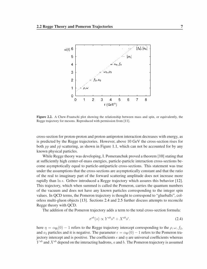
where α0 is the Regge trajectory intercept and α′ is the slope. Figure 2.2, a Chew-Frautschi
plot, shows four Regge trajectories: that of the ρ, ω, f2,and a2 particles. The trajectories
are degenerate, which did not necessarily have to happen.
As can be seen in the plot, the trajectory has a (nearly) universal slope and intercept,
independent of the particle family from which it originates.
Each of the Regge trajectories contributes to the total cross-section with the following
depedence on s:σab(s) ∝ sα(0)−1 (2.3)
where σab is the total interaction cross-section of particles a and b, and α(0) is the value
of the Regge trajectory at t = 0. In Figure 2.2 α(0) is roughly 0.5, which indicates a
cross-section decreasing with s. At√s less than 10 GeV the observed total scattering
2.2 Regge Theory and Pomeron Trajectories 7
Figure 2.2. A Chew-Frautschi plot showing the relationship between mass and spin, or equivalently, the
Regge trajectory for mesons. Reproduced with permission from [11].
cross-section for proton-proton and proton-antiproton interaction decreases with energy, as
is predicted by the Regge trajectories. However, above 10 GeV the cross-section rises for
both pp and pp scattering, as shown in Figure 1.1, which can not be accounted for by any
known physical particles.
While Regge theory was developing, I. Pomeranchuk proved a theorem [10] stating that
at sufficiently high center-of-mass energies, particle-particle interaction cross-sections be-
come asymptotically equal to particle-antiparticle cross-sections. This statement was true
under the assumptions that the cross-sections are asymptotically constant and that the ratio
of the real to imaginary part of the forward scattering amplitude does not increase more
rapidly than ln s. Gribov introduced a Regge trajectory which assures this behavior [12].
This trajectory, which when summed is called the Pomeron, carries the quantum numbers
of the vacuum and does not have any known particles corresponding to the integer spin
values. In QCD terms, the Pomeron trajectory is thought to correspond to “glueballs”, col-
orless multi-gluon objects [13]. Sections 2.4 and 2.5 further discuss attempts to reconcile
Regge theory with QCD.
The addition of the Pomeron trajectory adds a term to the total cross-section formula:
σab(s) ∝ Y absη +Xabsǫ. (2.4)
here η = αIR(0) − 1 refers to the Regge trajectory intercept corresponding to the ρ, ω, f2,and a2 particles and it is negative. The parameter ǫ = αIP(0)− 1 refers to the Pomeron tra-
jectory intercept and is positive. The coefficients ǫ and η are universal coefficients whereas
Y ab andXab depend on the interacting hadrons, a and b. The Pomeron trajectory is assumed
2.2 Regge Theory and Pomeron Trajectories 8
to behave the same as the ρ, ω, f2, a2 trajectory, therefore it is assumed that
αIP(t) = 1 + ǫ+ α′IPt. (2.5)
Fits to existing data prefer values of
η = −0.45; ǫ = 0.081; α′IP = 0.25 GeV−2. (2.6)
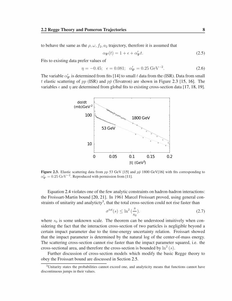
The variable α′IP is determined from fits [14] to small t data from the (ISR). Data from small
t elastic scattering of pp (ISR) and pp (Tevatron) are shown in Figure 2.3 [15, 16]. The
variables ǫ and η are determined from global fits to existing cross-section data [17, 18, 19].
10
100
0 0.05 0.1 0.15 0.2
53 GeV
1800 GeV
Ø ´ Î
¾
µ
Ø
´ Ñ Î
¾
µ
dσ/dt
(mb)GeV-2
|t| (GeV ) 2
Figure 2.3. Elastic scattering data from pp 53 GeV [15] and pp 1800 GeV[16] with fits corresponding to
α′IP = 0.25 GeV−2. Reproduced with permission from [11].
Equation 2.4 violates one of the few analytic constraints on hadron-hadron interactions:
the Froissart-Martin bound [20, 21]. In 1961 Marcel Froissart proved, using general con-
straints of unitarity and analyticty3, that the total cross-section could not rise faster than
σtot(s) ≤ ln2 (s
s0). (2.7)
where s0 is some unknown scale. The theorem can be understood intuitively when con-
sidering the fact that the interaction cross-section of two particles is negligible beyond a
certain impact parameter due to the time-energy uncertainty relation. Froissart showed
that the impact parameter is determined by the natural log of the center-of-mass energy.
The scattering cross-section cannot rise faster than the impact parameter squared, i.e. the
cross-sectional area, and therefore the cross-section is bounded by ln2 (s).Further discussion of cross-section models which modify the basic Regge theory to
obey the Froissart bound are discussed in Section 2.5.
3Unitarity states the probabilities cannot exceed one, and analyticity means that functions cannot have
discontinuous jumps in their values.

2.3 QCD and the Parton Model 9
2.3 QCD and the Parton Model
While Regge theory developed as a viable model for hadronic interactions, a new the-
ory pioneered by Gell-Mann and Zweig [22, 23] proposed an organizing principle for the
multitudes of recently discovered hadrons. It began with Gell-Mann’s eightfold way [22]
which used the symmetry group SU(3)4 to describe the masses and decays of the known
hadrons. The success of the SU(3) description led Gell-Mann and Zweig to propose that
hadrons were comprised of three fractionally charged fundamental particles, dubbed quarks
by Gell-Mann. In symmetry group terms, these quarks form the fundamental representa-
tion of the SU(3) group. Today these particles are known as u, d and s quarks and the
symmetry described by this approximate SU(3) theory is known as a “flavor symmetry”
and is valid in the limit of equal mass quarks.
Flavor SU(3) was challenged, however, by the discovery of the ∆++ baryon, which
had spin +32
and consisted solely of u quarks. Because quarks were believed to be spin12
fermions they could not simultaneously be in the same state as would be necessary to
produce a +32
particle. To solve this violation of the Pauli exclusion principle, Han, Nambu
and Greenberg proposed [24, 25] that the quarks had an additional SU(3) degree freedom,
which is now called color. All quarks carried color charge and the hadrons were composed
of combinations of which made the hadrons color singlets. The quark model had one prob-
lem: no quarks had ever been isolated in the laboratory and fractionally charged particles
had never been observed. Therefore many, including Gell-Mann, believed quarks were
only an abstract way of understanding nature.
Simultaneously, Feynman created the parton model, in which hadrons were composed
to quasi-free point-like particles he called partons [26]. He developed the theory in re-
sponse to results from the deep inelastic scattering experiments at the Stanford Linear Ac-
celerator (SLAC), in which 20 GeV electron beams were scattered off of liquid hydrogen
and liquid deuterium targets. These experiments were conceptually similar to the Ruther-
ford scattering experiment in which the structure of the atom was determined. A Feynman
diagram of the electron-proton interaction is shown in Figure 2.4. The electron emits a
photon5 with momentum four-vector q, which interacts with a parton carrying momentum
fraction, xp, of the proton. Measurements of the outgoing electron momentum translate
into measurements of the charge distribution and in the proton, called structure functions.
Higher order corrections give information about the gluon content of the proton.
At the same time as Feyman was developing the parton model, Bjorken postulated that
the structure functionsmeasured in inelastic scattering depended only on the dimensionless
ratio of the four-momentum transfer, q2, to the electron energy loss [27]. This behavior,
now called Bjorken scaling, is a consequence of a parton-like model, where the probe
particle, in this case an electron, acts incoherently on the proton constituents. A more
detailed discussion of deep-inelastic scattering experiments is given in Section 2.4. These
4SU(3) is the group of 3×3 matrices with unit determinant.5More generally, it emits an electroweak boson.

2.3 QCD and the Parton Model 10
measurements determined the parton distribution functions or PDFs which describe the
momentum faction of the proton carried by its constituent quarks and gluons.
Figure 2.4. Feynman diagram of deep inelastic scattering. The electron interacts with a valence quark via
a boson with four-vector q. The quark has a momentum fraction xp of the proton and by measuring the
scattered electron, xp can be determined.
Once Gross, Wilczek and Polizter [28, 29] showed that SU(3) leads to asymptotically
free gauge theories, i.e. the interactions between constituents becomes arbitrarily weak
for asymptotically large energies, SU(3) QCD became a viable and accepted theory of
strong interactions. In particular, asymptotic freedom allowed perturbation theory to be
used in the calculation of QCD processes, and lead to the factorization theorem which
states that the partonic scattering cross-section can be factorized from the PDFs [30, 31].
With factorization, cross-sections can be calculated via:
σ(P1, P2 → X) =∑
i,j
∫
dx1dx2fi(x1, Q2)fj(x2, Q
2)σ(i, j → X; x1P1, x2P2, Q2) (2.8)
where fi,j are the parton distribution functions for partons i and j, x1 and x2 are the momen-
tum fractions of parton i and j in proton 1 and 2, respectively, σ is the partonic cross-section
for X to be produced and Q2 is the momentum scale of the hard partonic interaction. Fac-
torization is not explicitly proven for all cross-sections, but it is currently one of the most
powerful tools for calculating cross-sections involving hadrons.
Asymptotic freedom and factorization are useful only in the large momentum transfer
limit. They do not provide calculational tools for low momentum transfer hadron-hadron
interactions. In fact, the opposite regime of arbitrarily low energy interactions gives rise to
the phenomena of quark confinement. Because QCD interactions become arbitrarily strong
at low energies, quarks and gluons cannot be observed individually, which is the principle
of confinement. This statement is not rigorously proven but it is generally accepted.
In Equation 2.8, both the PDFs and σ depend on the QCD coupling constant, αs. The
statement that QCD interactions become strong or weak is another way of saying that αs

2.4 Partonic Descriptions of the Pomeron 11
becomes large or small. The coupling depends on the momentum transfer of the interaction,
Q2, by the following expression at leading order in perturbation theory:
αs(Q2) =
12π
(33 − 2nf) ln (Q2/Λ2QCD)
(2.9)
where nf is the number of quark flavors with masses less than Q2, and ΛQCD is extracted
from fits to measurements of αs. The scale ΛQCD is considered to be the scale at which
QCD is non-perturbative. It is roughly 200 MeV, the same scale as the pion mass or hadron
size. For the majority of hadron-hadron scattering processes, Q2 in Equation 2.8 is the
momentum transfer between the protons. It is roughly ΛQCD and, consequently, αs ∼ 1.
When the expansion parameter, in this case αs, is & 1, perturbation theory is not applicable.
Because of these difficulties, QCD is unable to supply predictions for hadron-hadron cross-
sections.
2.4 Partonic Descriptions of the Pomeron
Since QCD was established as the theory of strong interactions, attempts have been
made to describe the Pomeron and Regge trajectory in terms of partons. The Pomeron
trajectory has no known associated particles, unlike the Regge trajectory of the ρ, ω, f2, and
a2. However, it can be described most simply as a two-gluon exchange process [32, 33, 34],
with higher order corrections arising as a ladder of gluon exchange, as shown in Figure 2.5.
Calculation of the Pomeron intercept, α(0), in this model [35] leads to a value of 1.0 which
is in reasonable agreement with the measured value of 1.08.
(a) (b)
Figure 2.5. Feynman of two-gluon exchange between partons at leading order (a) and with a ladder of higher
order gluon interactions (b).
High center-of-mass energy deep inelastic scattering experiments offer the opportunity
to directly probe the partonic description of the Pomeron. The HERA collider at the DESY
laboratory in Hamburg, Germany collides electrons and protons at a center of mass energy
of 318 GeV with the primary goal of precise measurements of the proton DPFs. At the
HERA experiments H1 and Zeus, events of the form p+ e→ e+X+ p as well as p+ e→

2.4 Partonic Descriptions of the Pomeron 12
e +X + Y with a large rapidity gap between X and Y , were observed [36, 37, 38]. Both
the intact proton and large rapidity gap are hallmarks of a diffractive interaction because
both signal the exchange of a color-less object. These events were selected and analyzed to
determine the diffractive parton distribution functions (DPDF).
Figure 2.6 shows an illustration of the p+ e→ e+X+ p, highlighting different factor-
ization schemes. Figure 2.6(a) shows a case where the diagram can be factorized based on
a hard scattering QCD collinear factorization theorem [39, 40]. This theorem states that for
a fixed final state proton momentum the DPDF can be obtained. In this case the DPDF is
dependent on the distribution of Pomerons in the proton, termed the Pomeron flux, and the
momentum transfer in the interaction. The Figure shows the momentum transfer q of the
probe particle, which interacts with a parton from a Pomeron with momentum fraction xIP
of the proton with a Pomeron flux, fIP/p. In this case the DPDF describing the probability
to find a parton with momentum fraction xp in the Pomeron is dependent on the Pomeron
momentum fraction of the proton, xIP. Figure 2.6(b) shows further factorization, which
has been determined empirically, where the proton vertex factorizes as well. When this
occurs, which the existing data suggest is applicable for low fractional proton losses, the
shape of the DPDF is independent of the proton four-momentum. In other words, xIP is in-
dependent of p and xp is independent of xIP. In this regime diffraction can be described by
the exchange of a Pomeron “parton” with universal parton densities [41]. The dependence
of these DPDFs on x and q2 can be determined using perturbative QCD as in the case of
standard PDFs.
(a) (b)
Figure 2.6. Illustration of p + e → e + X + p. (a) shows the the point of QCD collinear factorization and
(b) shows proton-vertex factorization.
The DPDFs determined at HERA fail badly at describing the Tevatron data on diffrac-
tive events [42], which would indicate their non-universality. However, reasonable agree-
ment is achieved once multiple parton interactions are taken into account via a ’rapidity gap
survival probability’, i.e. the probability that the rapidity gap in the diffractive interaction is
not spoiled by the non-diffractive interactions of other partons [42]. Due to the necessity of
adding a rapidity gap survival probability, the DPDFs cannot be used to predict the hadron-
2.5 Analytic Cross-Section Models 13
hadron cross-sections, however, they are useful in describing multi-particle production in
diffractive events, as discussed in Section 2.6.
2.5 Analytic Cross-Section Models
2.5.1 Total Cross-Sections
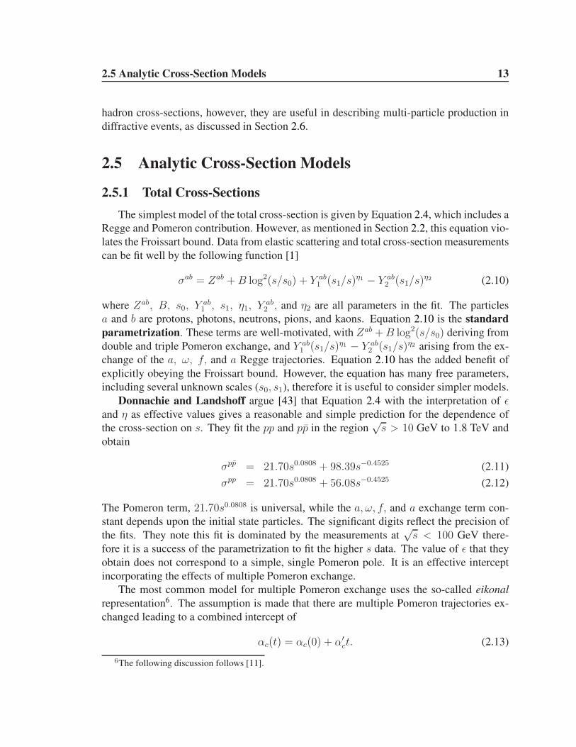
The simplest model of the total cross-section is given by Equation 2.4, which includes a
Regge and Pomeron contribution. However, as mentioned in Section 2.2, this equation vio-
lates the Froissart bound. Data from elastic scattering and total cross-section measurements
can be fit well by the following function [1]
σab = Zab +B log2(s/s0) + Y ab1 (s1/s)
η1 − Y ab2 (s1/s)
η2 (2.10)
where Zab, B, s0, Yab1 , s1, η1, Y
ab2 , and η2 are all parameters in the fit. The particles
a and b are protons, photons, neutrons, pions, and kaons. Equation 2.10 is the standard
parametrization. These terms are well-motivated, with Zab +B log2(s/s0) deriving from
double and triple Pomeron exchange, and Y ab1 (s1/s)
η1 − Y ab2 (s1/s)
η2 arising from the ex-
change of the a, ω, f, and a Regge trajectories. Equation 2.10 has the added benefit of
explicitly obeying the Froissart bound. However, the equation has many free parameters,
including several unknown scales (s0, s1), therefore it is useful to consider simpler models.
Donnachie and Landshoff argue [43] that Equation 2.4 with the interpretation of ǫand η as effective values gives a reasonable and simple prediction for the dependence of
the cross-section on s. They fit the pp and pp in the region√s > 10 GeV to 1.8 TeV and
obtain
σpp = 21.70s0.0808 + 98.39s−0.4525 (2.11)
σpp = 21.70s0.0808 + 56.08s−0.4525 (2.12)
The Pomeron term, 21.70s0.0808 is universal, while the a, ω, f, and a exchange term con-
stant depends upon the initial state particles. The significant digits reflect the precision of
the fits. They note this fit is dominated by the measurements at√s < 100 GeV there-
fore it is a success of the parametrization to fit the higher s data. The value of ǫ that they
obtain does not correspond to a simple, single Pomeron pole. It is an effective intercept
incorporating the effects of multiple Pomeron exchange.
The most common model for multiple Pomeron exchange uses the so-called eikonal
representation6. The assumption is made that there are multiple Pomeron trajectories ex-
changed leading to a combined intercept of
αc(t) = αc(0) + α′ct. (2.13)
6The following discussion follows [11].

2.5 Analytic Cross-Section Models 14
In the case of two exchanges αc(0) and α′c are given by
αc(0) = α1(0) + α2(0) − 1 (2.14)
α′c =
α′1α
′2
α′1 + α′
2
. (2.15)
This αc(t) corresponds to a partial wave amplitude,A, of the solution of the Yukawa poten-
tial, which can be expressed in terms of the impact parameter b and s. This is the eikonal
representation. The amplitude is then expressed as a Fourier transform back to momentum
transfer space, and expanded in a Taylor series
A(s,−q2) = 2is
∫
d2b e−iq·b
(
χ− χ2
2!+χ3
3!· · · −χ
n
n!· ··)
(2.16)
where the nth χ term corresponds to n Pomeron exchanges. Then, with a guess on the form
of χ, or the eikonal, motivated by the exact expression for single Pomeron exchange, the
optical theorem can be used to relate A at t = 0, the forward scattering cross-section, to
σtot:
σtot ∝ log2(s/s0). (2.17)
Donnachie and Landshoff argue [43] that the effect of the multiple Pomeron exchanges
is weak because
• The same power of ǫ fits all available hadron-hadron and hadron-antihadron cross-
sections.
• A single Pomeron contribution satisfies the additive quark rule [44] which states that
Xab ∝ nanb (2.18)
where na and nb are the number of valence quarks in a and b, respectively. It is
observed that Xπp : Xpp ≈ 2 : 3.
There are several additional models to mention:
• Engel: This model is implemented in the PHOJET Monte Carlo [45, 46], discussed
in more detail in Section 2.6. It is based on the Dual Parton Model (see [47] for a re-
view) which employs topological expansion to calculate interaction cross-sections [48].
Topological expansion tackles the non-perturbative nature of QCD by taking the large
N limit, where N refers to either the number of colors or quark flavors in the theory,
and using 1/N as the expansion parameter. The resulting diagrams are associated
with various topologies (plane, cylinder, torus, etc.) which correspond directly to
diagrams used in Reggeon Field Theory (RFT) [49]. Using RFT, the cross-sections
for collisions of Pomerons with hadrons and Pomerons with Pomerons can be cal-
culated. This description is valid in the regime where s is large compared to t. To

2.5 Analytic Cross-Section Models 15
[GeV]s
2103
10 410
[m
b]
tot
σ
0
20
40
60
80
100
120
140
160
180
200Single Pomeron Pole
Double Pomeron PoleBlockStandardCDFpp Data
Datapp
Single Pomeron Pole
Double Pomeron PoleBlockStandardCDFpp Data
Datapp
Figure 2.7. Proton-proton and proton-antiproton total cross-section as a function of√
s and fits. Single
Pomeron Pole refers to the standard Donnachie and Landshoff parametrization, Double Pomeron Pole refers
to the Donnachie and Landshoff model with the addition of a hard Pomeron. The Standard parametrization
uses a multiPomeron exchange approach. The Block and CDF parametrization are explained in the text. Data
from [1].
explain the rising cross-section and kinematic distributions, PHOJET uses an eikon-
alized hard and soft Pomeron with an explicit pT cutoff between the two of approx-
imately 3 GeV [50]. This description, with the explicit addition of Pomeron loops
and triple Pomeron exchanges, automatically leads to a cross-section which obeys
the Froissart bound.
• Khoze, Martin and Ryskin: This model [51] uses perturbative QCD in the high
parton transverse momentum, kt, region. BKFL [52, 53] evolution is used to evolve
the parton densities, which orders the partons in terms of log 1x
where x is Bjorken
x. The BKFL approach gives a candidate for a Pomeron in terms of multiple gluon
exchange. The model is then extended to the low kT region where multiple Pomeron
interactions are included using RFT. In this approach, the hard Pomeron contribution
can be smoothly matched to the soft Pomeron contribution.
• Block: In [54] two models are used to fit existing total cross-sections which yield
comparable results. The first is an eikonal fit inspired by QCD. In this model, the
dominant eikonal term is given by a factorized eikonal
χ(s, b) = ξqq(s, b) + ξqg(s, b) + ξgg(s, b) (2.19)
= i[σqq(s)W (b;µqq) + σqg(s)W (b;√µqqµgg)
+σgg(s)W (b;µgg)] (2.20)

2.5 Analytic Cross-Section Models 16
where σij(s) are the partonic cross-sections for ij and W (b;µij) is the dipole form
factor of the proton.
The second fit model uses real analytic amplitudes which require that the ampli-
tudes used to calculate high-energy scattering cross-section are real functions which
map smoothly onto low-energy amplitudes. This is a classic, model independent
method [55]. It results in a cross-section of
σpp = B1 + C1E−ν1 +B2ln
γs− C2E−ν2 (2.21)
where B1(2), C1(2), ν1(2) and γ are fit parameters. The fits parameters are fixed by
low-energy scattering data.
• CDF parametrization: This expression [56] is a refit of the simple single-Pomeron
pole, using only the CDF measurement at 1.8 TeV and excluding the E710 measure-
ment.
σtot = 24.36 mb ·( s
GeV2
)ǫ
with ǫ = α(0)− 1 = 0.0808. This yields a cross section of σtot(7 TeV) = 101.9 mb.
• Donnachie and Landshoff Double Pomeron: Donnachine and Landshoff revisited
the possibility of a hard Pomeron after analyzing the HERA diffractive deep inelastic
scattering data [57]. Their new parametrization [58], which gives similar results to
the simple single pole, parametrizes the cross-section using both a soft and a hard
Pomeron
σtot = 24.22 mb ·( s
GeV2
)0.0667
+ 0.0139 mb ·( s
GeV2
)0.452
This formulation yields a cross section of σtot(7 TeV) = 120.5 mb. Although this
model has two Pomeron poles, it does not account for multiple-Pomeron interactions.
Figure 2.7 shows a subset of the predictions compared with the existing total cross-
section data. Most of the predictions only vary by 10% at LHC energies, however the
Double Pomeron diverges with respect to the other models at high energy. It is inconsistent
with the cosmic-ray data, but these data are model-dependent and have large errors so they
are not used in the fit.
2.5.2 Inelastic and Diffractive Cross-sections
Most predictions of the inelastic cross-section from analytic models are obtained by
applying the optical theorem to the total cross-section prediction to obtain the elastic cross-
section and then calculating
σinel = σtot − σel. (2.22)

2.5 Analytic Cross-Section Models 17
Applying the optical theorem to the single Regge pole model yields the following elastic
differential cross-section
dσel
dt(pp→ pp) =
σ2tot(pp)
16πe2(b
el0 +α′
IP ln s)t. (2.23)
Using Mueller’s generalization of the optical theorem [59], the single-diffractive dissocia-
tion cross-section can also be derived from the elastic cross-section
d2σSD
dtdM2(pp→ Xp) ∝ 1
M2X
(
s
M2X
)2(αIP(0)−1)
e2(bSD0 +α′
IP ln s
M2 )t (2.24)
where bSD0 is the slope parameter describing the t-dependence of the cross-section and
M is the invariant mass of the products of the dissociated proton, or diffractive mass. This
equation is the standard Donnachie and Landshoff formulation of the differential diffractive
cross-section and is the baseline for which most other models are compared to.
In the following the main features of the analytic models for the inelastic cross-section
predictions used in this thesis are briefly described. Some models are used for their predic-
tions of the inelastic cross-section, others for the differential diffractive event cross-section
and some for both. The existing data and several of the models are shown in Figure 2.8.
[GeV]s
1 10 2103
10 410
[m
b]
inel
σ
0
20
40
60
80
100strandoSchuler and Sj
Block and Halzen 2011Achilli et al.pp Data
Datapp
Figure 2.8. Proton-proton and proton-antiproton inelastic cross-section as a function of√
s and fits. Data
from [1].
• Schuler-Sjostrand: This model [60] directly uses Equation 2.4 as the total cross-
section. The elastic cross-section is derived using the optical theorem. It begins with

2.5 Analytic Cross-Section Models 18
Equation 2.24 but notes that it is only valid in a limited parameter space: M2X−m2
p <0.15s, where mp is the mass of the proton. It is also limited to small values of
t. In order to obtain a prediction of all t and MX it introduces “fudge factors” to
suppress production near the kinematic limits listed above. It also modifies the slope
parameter for double-diffractive dissociation to keep it from becoming too small.
In this approach the asymptotic behaviors of the diffractive cross-sections have the
following energy dependence
σSD ∝ ln (ln s) (2.25)
σDD ∝ ln s(ln (ln s)) (2.26)
• Khoze, Martin and Ryskin: The details of the total cross-section predictions for
this model [51] are discussed in the previous subsection. The inelastic cross-section
is obtained by the optical theorem. The differential diffractive cross-sections are
calculated explicitly. In the intermediate diffractive mass range, the diffractive cross-
section is similar to a standard Donnachie and Landshoff approach like in Equa-
tion 2.24. There is a suppression at low diffractive mass from the absorption of
soft-kt partons, which decreases the probability of dissociation. At high mass there
is an increase of high-kt partons, leading to an increase in the cross-section. This
model is used for inelastic cross-section predictions.
• Achilli et. al.: This model [61] provides an explicit calculation of the inelastic cross-
section. It is calculated on the assumption that hadron-hadron scattering arises from
independently-distributed multiple-parton interactions. The inelastic cross-section is
then dependent on the average number of collisions, n(b, s), which is calculated in
an eikonalized model as a function of the impact parameter b and s. n is divided into
a hard and soft component where the hard component is calculated in perturbative
QCD, giving rise to mini-jets. The soft component is modeled in two different frame-
works; one Regge-inspired, the other based on soft gluon kt resummation. There is
no separate differential diffractive event cross-section.
• Berger and Streng: This model [62, 63] is only used to give a prediction for the
differential diffractive mass distribution. It uses a power law dependence of the cross-
section on the diffractive mass, similar to the Donnachie and Landshoff model, with
α(0) > 1. Unlike the Donnachie and Landshoff model, the t-dependence of the
differential cross-section is an exponential depending on MX .
• Bruni and Ingleman: This model [64] is only used for a prediction of the differential
diffractive mass spectra. It predicts a Pomeron with α(0) = 1, leading to a strictly
flat dependence of the cross-section on M2X , i.e. dσSD
dM2X
= const.. The t-dependence
of the cross-section is the sum of two exponential functions.
In this thesis the dimensionless unit ξ =M2
X
sis used to describe the differential diffrac-
tive cross-section. In the case of double-diffraction, ξ refers to the larger mass dissociation

2.6 Monte Carlo Models 19
system. Figure 2.9 shows the ξ distributions7, normalized to unit area, for SD and DDevents as predicted by the models listed above which have differential diffractive cross-
sections. In addition, there are four variations of ǫ and α′ in the Donnachie and Landshoff
models. Although ǫ and α′ are relatively well constrained by previous cross-section mea-
surements, the large uncertainty in the diffractive event dynamics justifies varying them
for the purposes of the acceptance calculations. Figures 2.9(a) and 2.9(b) show that the
Engel and Schuler-Sjostrand models predict higher average diffractive mass than the other
models. The power-law based models with α(0) > 1 are strongly peaked towards low
diffractive mass. Figures 2.9(c) and 2.9(d) show that the variations in ǫ and α′ have rel-
atively little effect on the diffractive mass spectra relative to the variations with the other
models.
2.6 Monte Carlo Models
By necessity, Monte Carlo models divide inelastic proton-proton interactions into three
or four categories: non-diffractive events and two or three types of diffractive events. These
classifications allow the generators to give predictions of exclusive quantities such as the
final state particle multiplicities and momenta. The analysis presented in this thesis is sen-
sitive to the dynamics of diffractive events, therefore predictions of the final state properties
of these events is necessary.
Two Monte Carlo generators are used: PYTHIA and PHOJET [45, 46]. Additionally,
two different versions of PYTHIA, 6.421 [65] and 8.135 [66], are considered. They use the
same Schuler-Sjostrand cross-section model for the diffractive processes, but differ in the
fragmentation once a value of M2X(Y ) and t are chosen. The cross-sections implemented
in PYTHIA and PHOJET for the individual processes are given in Table 2.1. It can be seen
that there are significant differences in the diffractive contributions. PHOJET additionally
includes central diffractive (CD) events where the protons do not dissociate but a central
system of particles is created by the Pomeron interactions.
The PYTHIA generator models non-diffractive pp interactions by first calculating a par-
tonic cross-section at leading order (2→2) in perturbation theory. The parton momentum
are picked using the proton PDFs, as indicated in Equation 2.8. Then it uses parton showers
to evolve the final state partons from the scale used in the partonic cross-section calculation
to a low scale cut-off. The evolution models the radiation of gluons (q → qg) and gluon
splitting (g → gg, g → qq) in the soft and collinear emission regime. This emission is
also modeled in the initial state via the parton PDFs. Once the emission reaches the cut-
off scale, which is a tunable parameter in the Monte Carlo generator, phenomenological
models are used to form the partons into color singlet hadrons. PYTHIA uses the Lund
7For technical reasons, which are described in more detail in Chapter 3, the ξ values plotted in Figure 2.9
are calculated from the final state particles produced by a Monte Carlo model. The particle production for
different Monte Carlo generators is discussed in detail in Section 2.6, but differences in the modeling of the
particle production have little effect on the resulting ξ distributions.

2.6 Monte Carlo Models 20
)ξ(10
log
8 7 6 5 4 3 2 1 0
Eve
nt
Fra
ctio
n
0
0.005
0.01
0.015
0.02
0.025
0.03
0.035strandoSchuler and Sj
Engel
Bruni and Ingelman
Berger and Streng2
’ = 0.25 GeVα = 0.085,∈DL
SD
(a)
)ξ(10
log
8 7 6 5 4 3 2 1 0
Eve
nt
Fra
ctio
n
0
0.005
0.01
0.015
0.02
0.025
0.03
0.035
0.04 strandoSchuler and SjEngel
Bruni and Ingelman
Berger and Streng2
’ = 0.25 GeVα = 0.085,∈DL
DD
(b)
)ξ(10
log
8 7 6 5 4 3 2 1 0
Eve
nt
Fra
ctio
n
0
0.005
0.01
0.015
0.02
0.025
0.03
0.035
0.042
’ = 0.25 GeVα = 0.06, ∈DL 2
’ = 0.25 GeVα = 0.10, ∈DL 2
’ = 0.10 GeVα = 0.085,∈DL 2
’ = 0.40 GeVα = 0.085,∈DL
SD
(c)
)ξ(10
log
8 7 6 5 4 3 2 1 0
Eve
nt
Fra
ctio
n
0
0.005
0.01
0.015
0.02
0.025
0.03
0.035 2’ = 0.25 GeVα = 0.06, ∈DL
2’ = 0.25 GeVα = 0.10, ∈DL
2’ = 0.10 GeVα = 0.085,∈DL
2’ = 0.40 GeVα = 0.085,∈DL
DD
(d)
Figure 2.9. ξ distribution for SD (left) and DD (right) events at√
s = 7 TeV comparing different ξ spectra as
described in the text. (a) and (b) compare the distributions for the basic models used to assess the dependence
of the cross-section of diffractive mass. (a) and (b) show variations of the Donnachie and Landshoff model
when varying ǫ and α′.
string model [67], in which color flux tubes are stretched between quark and anti-quark
pairs and are broken by the formation of a new qq pair; if the energy of the system is low
enough mesons are formed, otherwise new flux tubes are stretched between the q(q) from
the old pair and the q(q) of the new pair. Diquarks and anti-diquark pairs can also be pro-
duced to form baryons. Once all of the partons have been combined into color singlets,
fragmentation is finished.
PYTHIA uses QCD 2 → 2 processes to model non-diffractive interactions for both
PYTHIA 8 and PYTHIA 6. The two generators differ in some of the treatment of the color
connection between the initial and final states and in the tuning of the modeling parameters.
For diffractive processes, fragmentation for a particular value of M and t are very different
between the two.
• PYTHIA 6 only allows for “soft”, i.e. non-perturbative, fragmentation of diffractive
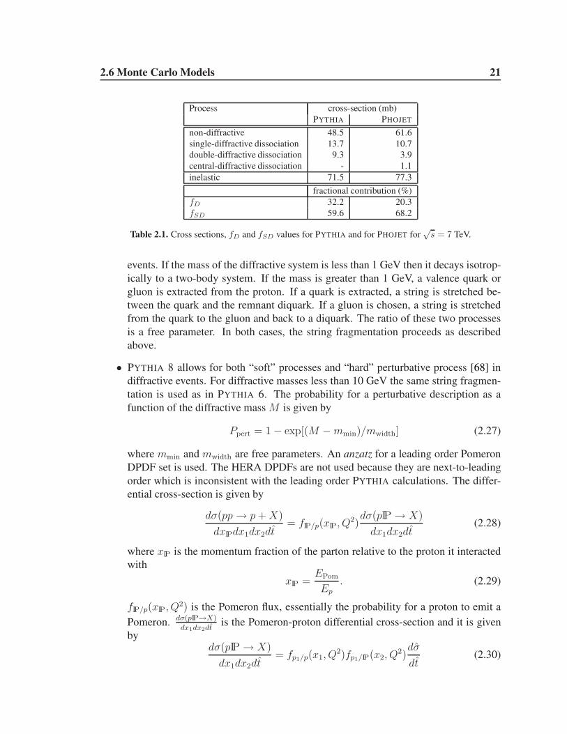
2.6 Monte Carlo Models 21
Process cross-section (mb)
PYTHIA PHOJET
non-diffractive 48.5 61.6
single-diffractive dissociation 13.7 10.7
double-diffractive dissociation 9.3 3.9
central-diffractive dissociation - 1.1
inelastic 71.5 77.3
fractional contribution (%)
fD 32.2 20.3
fSD 59.6 68.2
Table 2.1. Cross sections, fD and fSD values for PYTHIA and for PHOJET for√
s = 7 TeV.
events. If the mass of the diffractive system is less than 1 GeV then it decays isotrop-
ically to a two-body system. If the mass is greater than 1 GeV, a valence quark or
gluon is extracted from the proton. If a quark is extracted, a string is stretched be-
tween the quark and the remnant diquark. If a gluon is chosen, a string is stretched
from the quark to the gluon and back to a diquark. The ratio of these two processes
is a free parameter. In both cases, the string fragmentation proceeds as described
above.
• PYTHIA 8 allows for both “soft” processes and “hard” perturbative process [68] in
diffractive events. For diffractive masses less than 10 GeV the same string fragmen-
tation is used as in PYTHIA 6. The probability for a perturbative description as a
function of the diffractive mass M is given by
Ppert = 1 − exp[(M −mmin)/mwidth] (2.27)
where mmin and mwidth are free parameters. An anzatz for a leading order Pomeron
DPDF set is used. The HERA DPDFs are not used because they are next-to-leading
order which is inconsistent with the leading order PYTHIA calculations. The differ-
ential cross-section is given by
dσ(pp→ p+X)
dxIPdx1dx2dt= fIP/p(xIP, Q
2)dσ(pIP → X)
dx1dx2dt(2.28)
where xIP is the momentum fraction of the parton relative to the proton it interacted
with
xIP =EPom
Ep. (2.29)
fIP/p(xIP, Q2) is the Pomeron flux, essentially the probability for a proton to emit a
Pomeron.dσ(pIP→X)
dx1dx2dtis the Pomeron-proton differential cross-section and it is given
bydσ(pIP → X)
dx1dx2dt= fp1/p(x1, Q
2)fp1/IP(x2, Q2)dσ
dt(2.30)

2.6 Monte Carlo Models 22
where fp1/p(IP)(x1(2), Q2) is the proton (Pomeron) PDF for parton 1(2), with momen-
tum fraction x1(2) of the proton (Pomeron) and dσdt
is the partonic cross-section for the
two extracted partons. Figure 2.10 illustrates these quantities. In order to normalize
the Pomeron flux, an effective Pomeron-proton cross-section, σIPp is needed. It is
a tunable parameter in the event generation which controls the number of multiple
interactions in the event.
Figure 2.10. A single-diffractive dissociation event. pi,j are the momenta of the initial state protons. A
Pomeron with momentum fraction xIP is extracted from pi. A parton from pj is extracted with momentum
fraction xp1and interacts with a gluon from the Pomeron with a momentum fraction xg of the Pomeron. X
is the dissociation system and p′i is the momentum of the scattered proton.
Once the parton interaction has been described, parton showering and fragmentation
proceed as in the non-diffractive case.
The PHOJET model uses the Dual Parton Model, as mentioned in Section 2.5 for “soft”
interactions and perturbative QCD for “hard” interactions. The two are separated by a
momentum cut-off, pcut−offT . The perturbative treatment is similar to PYTHIA for non-
diffractive events. The “soft” interactions are treated using Reggeon Field Theory. The
number of soft and hard interactions in an event is given by
σ(ns, nh, s) =
∫
d2B(2χs)
ns
ns!
(2χh)nh
nh!e−2(χs+χh) (2.31)
where the χs and χh eikonals are functions of s and B, the impact parameter representation
of the soft and hard Pomeron. In RFT, the multiplicity of an event is obtained by using the
optical theorem to “cut” the diagram associated with the Pomeron exchange. The cross-
section for a particular number of cuts is given by the Gribov-Regge calculus [69]. In this
formulation there are few free parameters and it naturally leads to “hard” interactions in
diffractive events by the inclusion of the hard Pomeron.
Figures 2.11, 2.12, and 2.13 show the multiplicity, η distribution and pT distributions
of the three generators for each subprocess. It can be seen that for the non-diffractive pro-
cesses, PYTHIA 6 has the highest peak multiplicity and hardest pT spectrum of the three

2.6 Monte Carlo Models 23
generators. PHOJET has a distinctly lower average multiplicity and a relatively similar pT
spectrum to PYTHIA 8 for the non-diffractive events. Large differences between the gen-
erators are evident in the single-dissociation events. In the multiplicity plots, the PYTHIA
generators have two distinct populations, although the PYTHIA 8 generator has a signifi-
cantly higher multiplicity. PHOJET has a smooth distribution of multiplicities. PYTHIA 6
has approximately half as many particles per unit η. The momentum spectrum plots show
a striking difference between PYTHIA 6 and the other two generators, which shows that
the addition of a perturbative description of diffractive events drastically changes the event
kinematics. The double-dissociation plots show many of the same trends as the single-
dissociation plots. In particular the difference in the shape of the η distribution between the
generators is notable.
parN
0 50 100 150 200
par
dN
ev
dN
ev
N1
0
0.002
0.004
0.006
0.008
0.01
0.012
0.014 Pythia 8
Pythia 6
Phojet
ND
(a)
parN
0 50 100 150 200
par
dN
ev
dN
ev
N1
0
0.01
0.02
0.03
0.04
0.05
0.06
0.07Pythia 8
Pythia 6
Phojet
SD
(b)
parN
0 50 100 150 200
par
dN
ev
dN
ev
N1
0
0.005
0.01
0.015
0.02
0.025
0.03
0.035 Pythia 8
Pythia 6
Phojet
DD
(c)
Figure 2.11. Number of particles with pT >100 MeV per event for for ND (a), SD (b), and DD (c) events
comparing the PYTHIA 8, PYTHIA 6 and PHOJET generators at√
s = 7 TeV.
It is worth mentioning that the modeling of the non-diffractive process has been studied
in the context of measurements of charged particle multiplicities [70]. In these studies,
tuned PYTHIA 6 Monte Carlo events were seen to give the best agreement with the data.
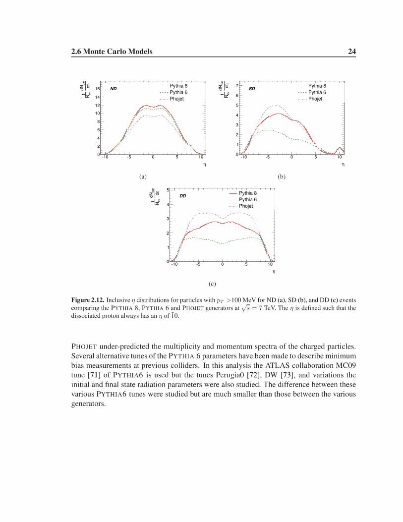
2.6 Monte Carlo Models 24
η
10 5 0 5 10
ηd
par
dN
ev
N1
0
2
4
6
8
10
12
14
16Pythia 8
Pythia 6
Phojet
ND
(a)
η
10 5 0 5 10
ηd
par
dN
ev
N1
0
1
2
3
4
5
6
7 Pythia 8
Pythia 6
Phojet
SD
(b)
η
10 5 0 5 10
ηd
par
dN
ev
N1
0
1
2
3
4
5Pythia 8
Pythia 6
Phojet
DD
(c)
Figure 2.12. Inclusive η distributions for particles with pT >100 MeV for ND (a), SD (b), and DD (c) events
comparing the PYTHIA 8, PYTHIA 6 and PHOJET generators at√
s = 7 TeV. The η is defined such that the
dissociated proton always has an η of 10.
PHOJET under-predicted the multiplicity and momentum spectra of the charged particles.
Several alternative tunes of the PYTHIA 6 parameters have been made to describe minimum
bias measurements at previous colliders. In this analysis the ATLAS collaboration MC09
tune [71] of PYTHIA6 is used but the tunes Perugia0 [72], DW [73], and variations the
initial and final state radiation parameters were also studied. The difference between these
various PYTHIA6 tunes were studied but are much smaller than those between the various
generators.
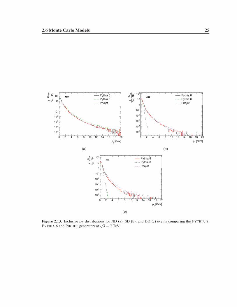
2.6 Monte Carlo Models 25
[GeV]T
p
0 2 4 6 8 10 12 14 16 18 20
Tdpp
ar
dN
ev
N1
510
410
310
210
110
1
10
210 Pythia 8
Pythia 6
Phojet
ND
(a)
[GeV]T
p
0 2 4 6 8 10 12 14 16 18 20T
dpp
ar
dN
ev
N1
510
410
310
210
110
1
10
210Pythia 8
Pythia 6
Phojet
SD
(b)
[GeV]T
p
0 2 4 6 8 10 12 14 16 18 20
Tdpp
ar
dN
ev
N1
510
410
310
210
110
1
10
210 Pythia 8
Pythia 6
Phojet
DD
(c)
Figure 2.13. Inclusive pT distributions for ND (a), SD (b), and DD (c) events comparing the PYTHIA 8,
PYTHIA 6 and PHOJET generators at√
s = 7 TeV.

26
CHAPTER 3
Inelastic Cross-Section Measurement
Overview
The general cross-section formula for the inelastic cross-section measurement is given
by:
σinel =N −NBG
ǫ× Ainel × L (3.1)
where N is the number of observed events, NBG is the number of background events,
Ainel is the acceptance, ǫ is the efficiency to select an event in the acceptance and L is
the luminosity. The particular event selection used in this analysis simply requires at least
two of the 31 MBTS counters to collect a charge of at least 0.15 pC. Events satisfying this
selection are collectively referred to as the inclusive sample.
As will be discussed in Chapter 10, the luminosity is measured using the beam scan-
ning technique first proposed by Simon van der Meer [74]. The uncertainty is at present
3.4% [75]. The determination of the number of selected events and the background is
straight-forward. However, the major challenge of the analysis is the determination of the
acceptance Ainel.
Ainel can be decomposed into the individual contributions to the inelastic cross section
as follows:
Ainel =AND
inclσND + ASDinclσSD + ADD
inclσDD + ACDinclσCD
σinel
(3.2)
= ANDincl
σND
σinel+ ASD
incl
σSD
σinel+ ADD
incl
σDD
σinel+ ACD
incl
σCD
σinel(3.3)
= ANDincl(1 − fD) + fD[ASD
inclfSD + ADDinclfDD + ACD
inclfCD] (3.4)
where
• ANDincl, A
SDincl, A
DDincl and, in the case of PHOJET, ACD
incl, are the acceptances of the event
selection for the ND, SD, DD and CD processes.

27
• fD is the fractional contribution of diffractive events to the inelastic cross-section:
fD = σSD+σDD+σCD
σinel. PYTHIA predicts 32% for fSD and PHOJET predicts 20%.
• fSD, fDD and fCD are the fractional contribution of SD, DD and CD to the diffractive
cross-section, e.g. fSD = 1 − fDD − fCD = σSD
σSD+σDD+σCD. PYTHIA predicts 60% for
fSD and PHOJET predicts 69%.
A priori,ANDincl, A
SDincl, andADD
incl, as well as fD and fSD are unknown. Monte Carlo models
give predictions for these values but they depend upon the underlying model assumed by
each generator. In order to reduce the impact of these unknown quantities, the analysis
takes two steps:
• First, the model dependence of the acceptance correction is limited by quoting the
measurement for a restricted ξ-range. In Chapter 2 ξ was defined as being equal toM2
swhere M was the invariant mass of the proton dissociation products. Because the
detector has finite resolution and acceptance, we cannot measure M (equivalently ξ)
directly, however the presence of an MBTS hit gives a lower limit on ξ. Therefore, ξis calculated for only the Monte Carlo models, which give access to the four-vectors
of all primary particles produced in an interaction. Primary particles are defined as
particles with a lifetime τ > 0.3 × 10⁻¹⁰s.
In order to avoid ambiguities in assigning a final state particle to an initial proton sys-
tem in the case of double diffractive dissociation, this measurement uses a modified
diffractive mass. After ordering all primary particles in pseudorapidity, the largest
pseudorapidity gap between adjacent particles is found. The mean pseudorapidity of
the two particles which define the gap is used to assign all particles with greater pseu-
dorapidity to one system and all particles with smaller pseudorapidity to the other.
This variable will correspond to the true diffractive mass except for rare cases where
the fluctuations in particle production produce a larger rapidity gap in the decay prod-
ucts of one system than between the two diffractive systems, which we term X and
Y . The system with the largest mass is by definition X , and ξ is defined to be M2X/s.
In the case of single-dissociationX is the system from the dissociated proton. In the
case of double-dissociation, ξ is defined by the larger of the two dissociation systems.
Figure 3.1 illustrates the definition.
Because ξ is defined using final state particles, it is slightly dependent on the under-
lying fragmentation model of the generator with which it was calculated. PYTHIA
6 and PYTHIA 8 have very different fragmentation models, but, as can be seen in
Figure 3.2, the differences lead to small discrepancies at high ξ.
ξ is closely related to the η of the particle in a dissociation system which starts the
rapidity gap. This value, ηmin, is shown in Figure 3.3 for all three generators. It can
be seen that in each case the dependence is linear with log ξ and that there is very
little difference in the dependence between generators. The average η−ξ relationship

28
Figure 3.1. A schematic illustration of MX , MY and ηmin in a double-dissociation event. The blue dashed
arrows indicate the smaller mass dissociation system, the solid red arrows indicate the higher mass system.
The two systems are defined by the largest rapidity gap in the event.
)ξ(10
log
8 7 6 5 4 3 2 1 0
Fra
ctio
n o
f E
ve
nts
0
0.002
0.004
0.006
0.008
0.01
0.012
0.014
0.016
0.018
0.02
0.022
0.024
Pythia 8
Phojet
Pythia 6
SD
(a)
)ξ(10
log
8 7 6 5 4 3 2 1 0
Fra
ctio
n o
f E
ve
nts
0
0.005
0.01
0.015
0.02
0.025
0.03
Pythia 8
Phojet
Pythia 6
DD
(b)
Figure 3.2. ξ distribution for SD (a) and DD (b) events at√
s = 7 TeV comparing the three Monte Carlo
generators. The difference in PYTHIA 6 and PYTHIA 8 is solely due to the difference in fragmentation
between the two models.
is given by
ln ξ = −∆η (3.5)
where ∆η is the difference between ηmin and η of the initial state proton system.
Equation 3.5 arises because the dissociation systems are highly boosted along z,
therefore the mass is related to the opening angle in θ. The maximum η-value of
the MBTS coverage of 3.84 restricts the measurement to the kinematic range of ξ >5 × 10⁻⁶.
• The second step the analysis takes to limit model-dependence is to use the data to
constrain fD by measuring the ratio of the number of events in a diffraction-enhanced
to inclusive event sample. The diffraction-enhanced sample is obtained by creating
a single-sided sample containing events with at least two hits on one side of the

29
Minη
6 4 2 0 2 4 6
)ξ(
10
log
7
6
5
4
3
2
1
0
0
0.001
0.002
0.003
0.004
0.005
0.006Phojet
Preliminary SimulationATLAS
(a)
Minη
6 4 2 0 2 4 6
)ξ(
10
log
7
6
5
4
3
2
1
0
0
0.001
0.002
0.003
0.004
0.005Pythia 8
Preliminary SimulationATLAS
(b)
Minη
6 4 2 0 2 4 6
)ξ(
10
log
7
6
5
4
3
2
1
0
0
0.001
0.002
0.003
0.004
0.005
0.006Pythia 6
Preliminary SimulationATLAS
(c)
Figure 3.3. ξ versus the η of the particle which defines the rapidity gap between the intact proton and
dissociation system in SD events(ηMin). PHOJET (a), PYTHIA8 (b) and PYTHIA6 (c) are shown.
MBTS in z and none on the other. This sample is expected to be dominated by
SD events, and DD events in which only one of the two dissociation systems has
ξ > 5 × 10⁻⁶. For example, PYTHIA predicts the fractional contribution of non-
diffractive events to the single-sided sample to be 1%, while PHOJET predicts 8%.
In the inclusive sample the non-diffractive process contributes about 74% and 80%
for PYTHIA8 and PHOJET, respectively. The acceptances are presented in detail
in Section 12.2. By taking the ratio of the single-sided to inclusive sample, and
comparing the measured value to the MC predictions, the allowed values of fD for
each MC model are constrained. The ratio, RSS, is given by
RSS =NSS
Nincl(3.6)
=Ainel
SS Ninel
AinelinclNinel
(3.7)
=Ainel
SS
Ainelincl
(3.8)

30
=AND
SSσND
σinel+ ASD
SSσSD
σinel+ ADD
SSσDD
σinel+ ACD
SSσCD
σinel
ANDincl
σND
σinel+ ASD
inclσSD
σinel+ ADD
inclσDD
σinel+ ACD
inclσCD
σinel
(3.9)
=AND
SS (1 − fD) + fD[ASDSS fSD + ADD
SS fDD + ACDSS fCD]
ANDincl(1 − fD) + fD[ASD
inclfSD + ADDinclfDD + ACD
inclfCD](3.10)
where the SS subscript indicates the single-sided event selection and the incl indicate
the inclusive event sample, as defined in Equation 3.2. To determine the relative
contribution of diffractive events, the A terms are taken from the models, as well as
fSD and fCD, and fD is adjusted until the model prediction matches the measured
value in data. Because the distinction between diffractive and non-diffractive events
varies model-by-model, fD is determined for each model separately.
Placing a cut on the diffractive mass modifies Equation 3.1 to
σ(ξ > 5 × 10⁻⁶) =(N −NBG)(1 − fξ<5×10⁻⁶)
ǫtrig × ǫsel ×L (3.11)
where 1 − fξ<5×10⁻⁶ corrects for the fraction of events in the inclusive sample which
have ξ < 5 × 10⁻⁶ , ǫsel is the event selection efficiency for events with ξ > 5 × 10⁻⁶, and
ǫtrig is the trigger efficiency with respect to the offline selection.
Using the tuned Monte Carlo simulation, ǫsel and fξ<5×10⁻⁶ are taken directly from the
MC and Equation 3.11 becomes
σ(ξ > 5 × 10⁻⁶) =(N −NBG)
ǫtrig × L × CMC (3.12)
where
CMC =1 − fξ<5×10⁻⁶
ǫsel. (3.13)
CMC is taken from Monte Carlo simulation (corrected for the MBTS efficiency mea-
sured in data), while the corrections for the trigger and backgrounds are determined from
data. The Donnachie and Landshoff model with ǫ = 0.085 and α′ = 0.25 GeV−2, hence-
forth referred to as the default model, is used to determine CMC and a variety of other
models, listed in Chapter 2.5, are used to determine any residual model uncertainty in these
correction factors.
The measurement of σinel(ξ > 5 × 10⁻⁶) is presented in Chapter 12. It is additionally
extrapolated to the full σinel using Ainel taken from the Donnachie and Landshoff model,
with a large uncertainty due to the model dependence.

31
CHAPTER 4
The Large Hadron Collider
The Large Hadron Collider (LHC) [76] was first conceived in the early 1990s and ap-
proved in preliminary form by the CERN council in 1994 on the heels of the US Super-
conducting Super Collider (SSC) failure. The appeal of the LHC was tied to the fact that it
was a bargain discovery machine; there was no need for a costly tunnel excavation because
one of a suitable size already existed for the CERN electron-positron collider, LEP. This
chapter reviews the motivation, design of the LHC and the running conditions from 2010.
4.1 Motivation
By the late 1980s, fundamental interactions of particles had revealed themselves to
be relatively simple and elegant. Nearlly all known phenomena could be explained by
SU(2)⊗U(1) electroweak theory and SU(3) QCD. The electroweak theory had once miss-
ing piece – a mechanism to break the symmetry and generate boson masses. The scale
associated with the symmetry breaking was calculated to be a few 100 GeV and in the
absence of a Higgs mechanism, in which a scalar field broke the symmetry, the weak in-
teractions were calculated to be come strong and violate unitarity at approximately 1 TeV.
And, while the fundamental particles had given no hint of substructure yet, if there were to
be substructure it was calculated that it would appear at 10−17 cm or ∼1 TeV. Therefore,
it was argued [77] that the next generation of collider needed to be in the multi-TeV scale,
ideally with a center-of-mass energy of 10 to 50 TeV for a proton-(anti)proton collider.
The SSC was proposed as a proton-antiproton collider with a√s of 40 TeV but it would be
relatively low luminosity. The LHC was put forward as a high luminosity machine at lower
energy. 14 TeV was roughly what could be expected given realistic magnet field strengths
and the diameter of the LEP tunnel. When the SSC was canceled in 1994, the LHC became
the next energy frontier machine.

4.2 Design 32
4.2 Design
The LHC is composed of over 1600 superconducting magnets arranged in a 26.7 km
tunnel under France and Switzerland. The tunnel, which was built in the late 1980s for
the Large Electron-Positron Collider (LEP), lies between 45m and 170m below the surface
of the earth. The original design, which has been preserved for the LHC, divided the ring
into eight arcs and eight straight sections to minimize energy loss from bremstralung by the
original electron and positron beams. There are eight possible interaction points on the ring,
four of which are in use for LHC experiments. ATLAS and CMS sit opposite each other
on the ring and are the designated discovery experiments. LHCb and ALICE are “low”
luminosity experiments investigating flavor physics and heavy ion collisions, respectively.
The LHC is designed to operate at a luminosity of 1034s−1cm−2 and a center of mass
energy,√s, of 14 TeV. The machine is filled with bunches of protons with a minimum
spacing of 25 ns. The revolution frequency of a bunch of protons is 11,245 Hz and there are
roughly 3600 possible bunch slots in the machine. When the bunch-spacing is 75 ns or less,
the beams are brought to collision at a crossing angle to reduce beam-beam interactions at
points other than the nominal collision point.
On September 19th, 2009 the LHC had an accident which caused extensive damage
to one sector of the ring and had significant implications for machine safety and beam
energy [78]. It delayed the start of the LHC for a year and limited the center-of-mass
energy to 7 TeV until improvements can be made to the machine. The incident is discussed
further in Section 4.2.3. Full energy (14 TeV) will be achieved in 2014.
4.2.1 Accelerator Chain
The CERN accelerator complex, shown in Figure 4.1, begins with a bottle of hydrogen
and ends with multi-TeV collisions. It uses a four accelerators to bring the protons from
rest to 450 GeV, the injection energy of the beam into the LHC. All of the pre-accelerators
were in use for physics programs at some point in CERN’s 50+ year history.
To start, electrons are stripped from the hydrogen atoms and the remaining protons
undergo the first stage of acceleration in the LINAC2, a linear accelerator commissioned
in 1978 to produce 50 MeV protons for the Proton Synchrotron Booster. The Booster
accelerates the protons to 1.4 GeV. It was built in 1972 and its RF system was recently
upgraded to accommodate the needed bunch frequency of the LHC. Ultimately, it sets the
bunch structure for the LHC because it is the first stage of bunched injection. The Booster
delivers its protons at 324 ns spacing to the Proton Synchrotron (PS), which is CERN’s
first synchrotron. Constructed in 1959, it uses conventional electromagnets to accelerate
protons to 26 GeV. The final stage in the chain is the Super Proton Synchrotron (SPS), a
450 GeV accelerator which was home to the W and Z bosons discoveries in the 1980s.
The SPS is filled with 72 bunches at a time from the PS. It accelerates the protons to 450
GeV and sends up to 72 bunches at a time in the form of a bunch-trains into the LHC. Once
all of the bunches are in the LHC the current is ramped in the magnets, until the beams are
4.2 Design 33
Figure 4.1. The CERN accelerator complex.[79]
at collision energy.
4.2.2 Magnets
The heart of the LHC is its enormous superconducting magnet system, consisting pri-
marily of 15 m long dipole and quadrupole magnets. The dipole magnets are responsible
for the bending of the beams, while quadrupole magnets provide focusing. Higher mul-
tipole corrector magnets are interspersed along the beamline. Acceleration is achieved
through superconducting 400 MHz RF cavities.
The design of the magnets was driven by two factors, one physics based, the other con-
struction constrained. To achieve the high luminosity needed to produce the rare processes
the LHC intends to find, a proton anti-proton machine is not feasible due to the difficulty of
accumulating a significant number of anti-protons. Proton beams cannot counter-circulate
in the same vacuum chamber or beam-pipe as proton and anti-proton beams can, therefore
separate magnetic fields and vacuum chambers are needed. However, the LEP tunnel is too
narrow to fit two separate magnet systems, therefore a twin-bore design was adopted [80].
The LHC dipole design is shown in Figure 4.2. Two magnets and beam-pipes sit in the
same cryostat and cold-mass which is cooled by superfluid helium to a temperature of

4.2 Design 34
1.7K. The LHC constitutes the largest, coldest cryogenic system in the world.
The magnets are made of niobium titanium (NbTi) cables and have fields of up to 8 T at
a current of nearly 12 kA. The total stored energy of the beams and current in the magnets
is over 1 GJ which can be dangerous to the machine if it is relased in an uncontrolled way,
such as through a quench. A quench occurs when the normally superconducting magnets
loose their superconductivity, suddenly causing a large build up of resistance where the
quench began. A quench protection system (QPS) based on monitoring changes in volt-
age between (nominally identical) magnets is in place to safegaurd the machine. When a
quench is detected it usies heaters mounted on the magnet coils to raise the temperature and
create an extended normally conducting zone along the length of the entire magnet and its
neighbors. This process safely dissipates the energy in a large volume. In order to protect
the machine and the detectors in the event of loss of control of the beam, a beam dump
system is in place to extract the beam quickly and safely. It is triggered by beam conditions
monitors at multiple points along the ring which look for an excess of interactions near the
beamline. The beam can be extracted in O(100 µs).
Figure 4.2. A cross section of the LHC dipole illustrating the twin-bore design.
Near the interaction regions, inner triplet magnets, which are a series of three quadrupole
magnets with alternating gradients, bring the beams into collisions. The optics at the inter-
action region can be adjusted for different beam sizes and energies.

4.3 2010 Run Conditions 35
4.2.3 The September 19th Incident
Commissioning of the LHC began in the fall of 2008 with the establishment of single
beam circulation at injection energy on September 10th. Shortly thereafter problem with
a transformer suspended beam tests for several days. While the transformer was being re-
placed, experts performed powering tests in a section of the machine, Sector 3-4, to ramp
the current in the magnets up to 9.3 kA, the current associated with 5 TeV beams. During
the test a quench developed between two magnets in a region called a bus bar splice. An
electrical arc occurred, which dissipated more the 4 MW in one second [78]. Part of the bus
bar was vaporized and the helium enclosure was punctured, allowing the the superfluid he-
lium to enter the cryostat vacuum insulation volume. The cyrostat subsequently punctured,
leading to a rapid increase in the helium pressure. The pressure in the insulation volume
rose as high as 0.8 MPa, ripping some of the 35 ton magnets from their support jacks and
blowing off the door of the tunnel in that sector. In total, 755m of the tunnel was damaged.
Reports after the incident [78] indicated that the initial arc was caused by poor soldering in
the bus bar which failed. The QPS did not monitor the bus bars, which is why the quench
developed undetected.
Recovery from this incident took over a year. In addition to replacing or refurbishing the
damaged magnets, the QPS system was upgraded to include monitoring of the splices, more
pressure release valves were installed and other potentially problematic bus bar splices
were identified and fixed. However, it was determined [81] that until significant upgrade
to the machine to fix more splices and further improve the machine protection systems, the
machine energy would be limited. In January, 2011 it was decided [82] that the LHC would
run at 7 TeV until the end of 2012, after which there would be a 1.5 year shutdown to make
the improvements. In 2014 the LHC will come online at 14 TeV.
4.3 2010 Run Conditions
Because 2010 was largely a commissioning period, the LHC running conditions were
significantly different than the design parameters discussed above. Due to machine safety
concerns in the wake of the September 19th incident, the center-of-mass energy was limited
to 7 TeV. The initial running period in March and April, which this thesis primarily con-
cerns, saw instantaneous luminosities of 1027cm−2s−1, while the peak luminosity, which
was achieved in November, was 2.1×1032cm−2s−1. Figure 4.3 shows the evolution of both
the peak instantaneous and integrated luminosity over the 2010 7 TeV run period. Com-
missioning began with only one colliding bunch pair in ATLAS; in the fall the LHC was
operating with bunch trains with 75 ns bunch spacing and a total of 368 colliding bunches.
Table 4.1 compares the LHC machine parameters in the early 2010 7 TeV running, late
2010 running and nominal 14 TeV running. It is notable that the machine is already running
at full bunch intensity. The increase to 1034 cm−2s−1 will come from increasing the number
of bunches in the machine and narrowing the bunch size. The bunch size is determined in

4.3 2010 Run Conditions 36
Early 2010 Late 2010 Nominal√s [TeV] 7 7 14
nb 1-2 348 2808
Np 1.1×10¹⁰ 1.1× 10¹¹ 1.15× 10¹¹
L[cm−2s−1] 1028 1032 1034
β∗ [m] 11 3.5 0.6
Crossing angle [µrad] 0 200 285
Table 4.1. Comparison of the LHC machine conditions in early 2010, late 2010 and nominal design pa-
rameters. Early 2010 conditions were the same as for the run for the cross-section measurement. nb is the
number of colliding bunches in the machine, Np is the number of protons per bunch or bunch intensity, and
L is the average instantaneous luminosity. β∗ is related to the amplitude function of the beam envelope at the
interaction point. The crossing angle refers to the angle of the beams with respect to the nominal beamline at
the collision point.
part by β∗, which determines the amplitude function of the beams at the interaction point.
Initially beams collided head-on with no crossing angle at the interaction point, but once
the bunch spacing became small with respect to the region that the two beams share the
same beam-pipe, a crossing-angle was introduced to reduce beam-beam interactions.
Day in 2010
24/03 21/0419/05 16/06 14/07 11/0808/0906/10 03/11
]1
s2
cm
30
Pe
ak L
um
ino
sity [
10
310
210
110
1
10
210
310
410 = 7 TeVs ATLAS Online Luminosity
LHC Delivered
1 s2 cm32
10×Peak Lumi: 2.1
(a)
Day in 2010
24/03 21/0419/05 16/06 14/07 11/0808/0906/10 03/11
]1
To
tal In
teg
rate
d L
um
ino
sity [
pb
510
410
310
210
110
1
10
210
310
410
Day in 2010
24/03 21/0419/05 16/06 14/07 11/0808/0906/10 03/11
]1
To
tal In
teg
rate
d L
um
ino
sity [
pb
510
410
310
210
110
1
10
210
310
410 = 7 TeVs ATLAS Online Luminosity
LHC Delivered
ATLAS Recorded
1Total Delivered: 48.9 pb1
Total Recorded: 45.0 pb
(b)
Figure 4.3. Peak luminosity by day (a) and total integrated luminosity by day (b) in 2010.
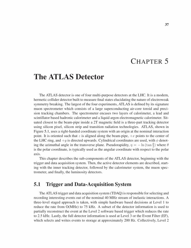
37
CHAPTER 5
The ATLAS Detector
The ATLAS detector is one of four multi-purpose detectors at the LHC. It is a modern,
hermetic collider detector built to measure final states elucidating the nature of electroweak
symmetry breaking. The largest of the four experiments, ATLAS is defined by its signature
muon spectrometer which consists of a large superconducting air-core toroid and preci-
sion tracking chambers. The spectrometer encases two layers of calorimeter, a lead and
scintillator based hadronic calorimeter and a liquid argon electromagnetic calorimeter. Sit-
uated closest to the beam-pipe inside a 2T magnetic field is a three-part tracking detector
using silicon pixel, silicon strip and transition radiation technologies. ATLAS, shown in
Figure 5.1, uses a right-handed coordinate system with an origin at the nominal interaction
point. It is oriented such that z is aligned along the beam-pipe, +x points to the center of
the LHC ring, and +y is directed upwards. Cylindrical coordinates are used, with φ denot-
ing the azimuthal angle in the transverse plane. Pseudorapidity, η = − ln (tan θ2) where θ
is the polar coordinate, is typically used as the angular coordinate with respect to the polar
axis.
This chapter describes the sub-components of the ATLAS detector, beginning with the
trigger and data acquisition system. Then, the active detector elements are described, start-
ing with the inner tracking detector, followed by the calorimeter system, the muon spec-
trometer, and finally, the luminosity detectors.
5.1 Trigger and Data-Acquisition System
The ATLAS trigger and data acquisition system (TDAQ) is responsible for selecting and
recording interesting events out of the nominal 40 MHz stream of inelastic interactions. A
three-level staged approach is taken, with simple hardware based decisions at Level 1 to
reduce the rate from O(MHz) to 75 kHz. A subset of the detector information is used to
partially reconstruct the event at the Level 2 software based trigger which reduces the rate
to 2.5 kHz. Lastly, the full detector information is used at Level 3 or the Event Filter (EF),
which selects and writes events to storage at approximately 200 Hz. Collectively, Level 2

5.1 Trigger and Data-Acquisition System 38
Figure 5.1. A diagram of the ATLAS detector indicating its sub-components [83].
and the EF are known as the High Level Trigger (HLT).
For the data used in this thesis, only the Level 1 trigger was used. The HLT was run in
“pass-through mode” where the algorithms ran and recorded their decisions, but all events
passing the Level 1 triggers were written to storage. At Level 1 algorithms implemented in
the calorimeter trigger (L1Calo) hardware identify electron, photon, tau and jet-like objects
and muon-like signatures are found in the muon trigger (MUCTP) hardware. At this point
only information from the calorimeters, muon system and forward detectors is used. When
a Level 1 object, is found a signal is sent to the workhorse of the Level 1 trigger, the Central
Trigger Processor (CTP). The CTP collates the trigger signals from all of the parts of the
detectors and forms multiplicities of objects. It additionally distributes the LHC clock,
event number and bunch-crossing identifier to the data acquisition system.
Using a trigger menu, the CTP either selects an event or rejects it. Rejection can occur if
a trigger menu item is not satisfied (e.g. the lowest muon threshold is not in the menu) or if
an item is satisfied but it is prescaled. Prescaling limits the bandwidth of a particular trigger
signature by only accepting every N th event, where N is the prescale. In the meantime, the
data acquisition system keeps the event information waiting for a trigger decision in buffers
in the detector readout electronics.
If the event is selected, the CTP sends a signal to the L1Calo and MUCTP which re-
tains information about the position of trigger objects, called regions-of-interest (ROI). A
software farm partially builds the event using the data stored in buffer in the ROI and the
Level 2 criteria are applied. If the Level 2 bit is passed then the data are taken off the

5.2 The Inner Detector 39
buffers for the entire detector and sent for full event building at the EF level. If an EF bit is
set, then the data are written to storage.
5.2 The Inner Detector
The Inner Detector (ID) provides charged-particle tracking in a 2T solenoidal field up
to |η| < 2.5. It is constrained by the following physics requirements:
• High quality momentum resolution for charged particles over a wide range of mo-
menta.
• Excellent position resolution for primary vertex finding and secondary vertex identi-
fication.
In order to achieve these requirements the following additional design requirement are
applied:
• Strong, uniform magnetic field - to make precise momentum measurements
• Minimal amount of material in the detector - to reduce multiple scattering and nuclear
interactions
• Radiation hard technologies - to withstand the radiation dose sustained at close radii
to the interaction point
• Low occupancy - to improve pattern recognition and detector performance in a high
multiplicity environment
• Mechanical stability - to ensure that the detector alignment does not vary significantly
with time.
ATLAS chose to satisfy these requirements using three technologies employed at different
radii of the detector, each of which has a specific purpose. Closest to the beam-pipe at
small radii is the three-layer Pixel detector, which provides the finest granularity measure-
ments and is crucial for precise vertex finding. The intermediate layer of the ID consists
of a four-layer silicon strip detector, which provides tracking through double-sided stereo-
axial layers. This design allows for high-quality tracking at lower cost than silicon pixels.
The outermost layer is a transition radiation tracker which uses thin tubes to provide, on
average, 32 additional measurements per track as well as electron-pion separation through
analysis of transition radiation. Figure 5.2 show the active elements of the barrel (|η| . 1).
Carbon fiber support structures are used throughout the detector to provide stability at low
material cost. Lastly, the detector is immersed in a 2T magnetic field generated by a thin,
superconducting solenoid. The field axis is along the z direction. Table 5.1 summarizes the
dimensions of each part of the Inner Detector system and 5.3 graphically illustrates them.

5.2 The Inner Detector 40
Figure 5.2. Cutaway of the ATLAS Inner Detector showing transverse barrel view. [83]
The material budget of the Inner Detector is shown in Figure 5.4 in both interaction
lengths, λ, and radiation lengths, X0. It can be seen that λ is dominated by the support
structures for most of the η range, while X0 is dominated by external services such as
cooling and electrical connections. The amount of material is significant, totaling almost 1
λ and 2.5 X0 at |η| =1.5. The region which is most important for the work in this thesis
is between |η| of 2 and 4. It is dominated by pixel detector cabling, cooling, and other
services.
5.2.1 Pixel Detector
The pixel detector is at the closest radius to the beam and therefore has the strictest
requirements on radiation hardness, occupancy, and precision. All of these requirements
are met, at least partially, by the use of a highly granular technology such as silicon pixels.
The effects of radiation damage are mitigated by the small leakage current of pixels. The
high granularity ensures low occupancy even at high charged particle multiplicities and
translates into more precise measurements, improving track parameter resolution.
The detector consists of three barrel layers and two three-layer end-caps. Each layer is
made of overlapping, identical silicon sensors mounted on modules, which are the building
blocks of the pixel detector. In total, 1744 modules are used in the full detector. In the
barrel, the modules have intrinsic resolutions of 10 µm in the plane transverse to the beam-
line and 115 µm in the longitudinal coordinate. In the end-caps, the precision coordinates
are in the z − φ direction and there is lower accuracy in the r direction.
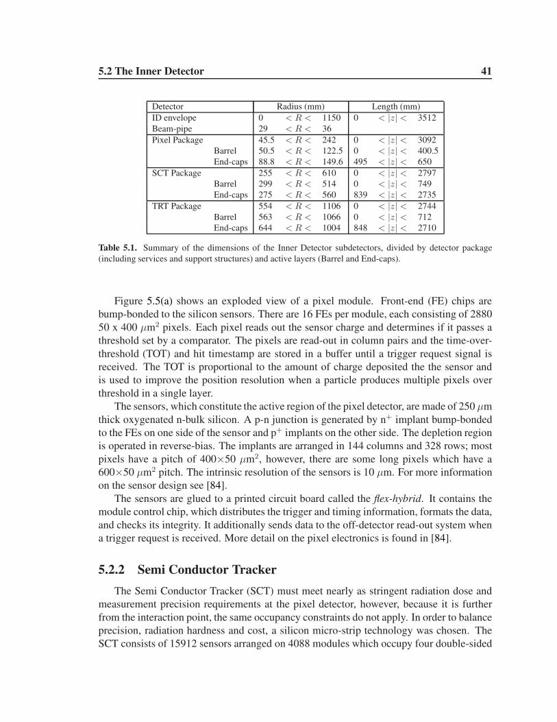
5.2 The Inner Detector 41
Detector Radius (mm) Length (mm)
ID envelope 0 < R < 1150 0 < |z| < 3512
Beam-pipe 29 < R < 36
Pixel Package 45.5 < R < 242 0 < |z| < 3092
Barrel 50.5 < R < 122.5 0 < |z| < 400.5
End-caps 88.8 < R < 149.6 495 < |z| < 650
SCT Package 255 < R < 610 0 < |z| < 2797
Barrel 299 < R < 514 0 < |z| < 749
End-caps 275 < R < 560 839 < |z| < 2735
TRT Package 554 < R < 1106 0 < |z| < 2744
Barrel 563 < R < 1066 0 < |z| < 712
End-caps 644 < R < 1004 848 < |z| < 2710
Table 5.1. Summary of the dimensions of the Inner Detector subdetectors, divided by detector package
(including services and support structures) and active layers (Barrel and End-caps).
Figure 5.5(a) shows an exploded view of a pixel module. Front-end (FE) chips are
bump-bonded to the silicon sensors. There are 16 FEs per module, each consisting of 2880
50 x 400 µm2 pixels. Each pixel reads out the sensor charge and determines if it passes a
threshold set by a comparator. The pixels are read-out in column pairs and the time-over-
threshold (TOT) and hit timestamp are stored in a buffer until a trigger request signal is
received. The TOT is proportional to the amount of charge deposited the the sensor and
is used to improve the position resolution when a particle produces multiple pixels over
threshold in a single layer.
The sensors, which constitute the active region of the pixel detector, are made of 250 µm
thick oxygenated n-bulk silicon. A p-n junction is generated by n+ implant bump-bonded
to the FEs on one side of the sensor and p+ implants on the other side. The depletion region
is operated in reverse-bias. The implants are arranged in 144 columns and 328 rows; most
pixels have a pitch of 400×50 µm2, however, there are some long pixels which have a
600×50 µm2 pitch. The intrinsic resolution of the sensors is 10 µm. For more information
on the sensor design see [84].
The sensors are glued to a printed circuit board called the flex-hybrid. It contains the
module control chip, which distributes the trigger and timing information, formats the data,
and checks its integrity. It additionally sends data to the off-detector read-out system when
a trigger request is received. More detail on the pixel electronics is found in [84].
5.2.2 Semi Conductor Tracker
The Semi Conductor Tracker (SCT) must meet nearly as stringent radiation dose and
measurement precision requirements at the pixel detector, however, because it is further
from the interaction point, the same occupancy constraints do not apply. In order to balance
precision, radiation hardness and cost, a silicon micro-strip technology was chosen. The
SCT consists of 15912 sensors arranged on 4088 modules which occupy four double-sided

5.2 The Inner Detector 42
Envelopes
Pixel
SCT barrel
SCT end-cap
TRT barrel
TRT end-cap
255<R<549mm|Z|<805mm
251<R<610mm810<|Z|<2797mm
554<R<1082mm|Z|<780mm
617<R<1106mm827<|Z|<2744mm
45.5<R<242mm|Z|<3092mm
Cryostat
PPF1
CryostatSolenoid coil
z(mm)
Beam-pipe
Pixelsupport tubeSCT (end-cap)
TRT(end-cap)
1 2 3 4 5 6 7 8 9 10 11 12 1 2 3 4 5 6 7 8
Pixel
400.5495
580
650749
853.8934
1091.5
1299.9
1399.7
1771.4 2115.2 2505 2720.200
R50.5R88.5
R122.5
R299
R371
R443R514R563
R1066
R1150
R229
R560
R438.8R408
R337.6R275
R644
R1004
2710848712 PPB1
Radius(mm)
TRT(barrel)
SCT(barrel)Pixel PP1
3512ID end-plate
Pixel
400.5 495 580 6500
0
R50.5
R88.5
R122.5
R88.8
R149.6
R34.3
Figure 5.3. An r − z view of a quarter of the Inner Detector, indicating the dimensions of each part of the
detector. PP1,PPB1 and PPF1 indicate the patch panels for the Inner Detector services [83].
barrel layers and two nine-layer end-caps. In the barrel, the modules [85] are arranged in
coaxial staves and the end-caps are perpendicular to the beam-line. A barrel module is
shown in Figure 5.5(b).
The sensors are based on a standard p-n junction in oxygenated silicon with AC-coupled
read-out strips. They are 6 cm long with a strip pitch of 80 µm. In the barrel, two sensors
are daisy-chained together, creating a single 12 cm unit. Each module has two 12 cm sensor
units glued to opposite sides of a base-board. The sensors are rotated at ±20 mrad around
the center of the module (40 mrad with respect to each other). This design results in 16 µm
position resolution in the r − φ plane. The end-cap modules have a very similar design.
Unlike the pixel read-out, which contains the TOT analog information, the SCT features
binary read-out. The hybrids consist of an integrated circuit with a pre-amplifier, signal
shaper and a discriminator which determines whether or not the charge collected in a strip
is over threshold. The hybrid also distributes the trigger and timing information as well as
sends the compressed and serialized data to the off-detector read-out system. More detail
on the SCT sensors and electronics is found in [85].
5.2.3 Transition Radiation Tracker
The Transition Radiation Tracker (TRT) is the outermost component of the Inner Detec-
tor and provides continuous tracking out to a radius of 1 m, improving the track resolution
considerably at low cost. It additionally provides electron-pion separation. It is separated
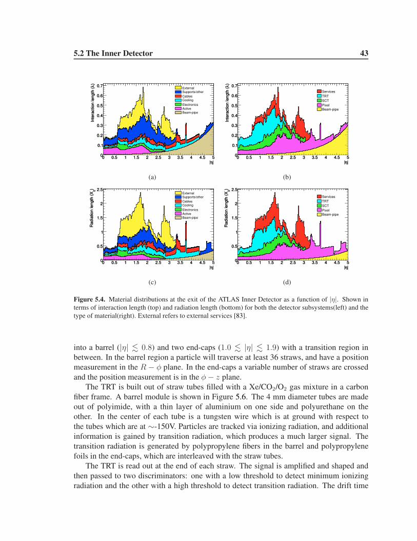
5.2 The Inner Detector 43
|η|0 0.5 1 1.5 2 2.5 3 3.5 4 4.5 5
)λ
Inte
ractio
n le
ng
th (
0
0.1
0.2
0.3
0.4
0.5
0.6
0.7
|η|0 0.5 1 1.5 2 2.5 3 3.5 4 4.5 5
)λ
Inte
ractio
n le
ng
th (
0
0.1
0.2
0.3
0.4
0.5
0.6
0.7ExternalSupports/other
CablesCooling
Electronics
ActiveBeam-pipe
(a)
|η|0 0.5 1 1.5 2 2.5 3 3.5 4 4.5 5
)λ
Inte
ractio
n le
ng
th (
0
0.1
0.2
0.3
0.4
0.5
0.6
0.7
|η|0 0.5 1 1.5 2 2.5 3 3.5 4 4.5 5
)λ
Inte
ractio
n le
ng
th (
0
0.1
0.2
0.3
0.4
0.5
0.6
0.7
Services
TRT
SCT
Pixel
Beam-pipe
(b)
|η|0 0.5 1 1.5 2 2.5 3 3.5 4 4.5 5
)0
Ra
dia
tio
n le
ng
th (
X
0
0.5
1
1.5
2
2.5
|η|0 0.5 1 1.5 2 2.5 3 3.5 4 4.5 5
)0
Ra
dia
tio
n le
ng
th (
X
0
0.5
1
1.5
2
2.5ExternalSupports/other
CablesCooling
Electronics
ActiveBeam-pipe
(c)
|η|0 0.5 1 1.5 2 2.5 3 3.5 4 4.5 5
)0
Ra
dia
tio
n le
ng
th (
X
0
0.5
1
1.5
2
2.5
|η|0 0.5 1 1.5 2 2.5 3 3.5 4 4.5 5
)0
Ra
dia
tio
n le
ng
th (
X
0
0.5
1
1.5
2
2.5
Services
TRT
SCT
Pixel
Beam-pipe
(d)
Figure 5.4. Material distributions at the exit of the ATLAS Inner Detector as a function of |η|. Shown in
terms of interaction length (top) and radiation length (bottom) for both the detector subsystems(left) and the
type of material(right). External refers to external services [83].
into a barrel (|η| . 0.8) and two end-caps (1.0 . |η| . 1.9) with a transition region in
between. In the barrel region a particle will traverse at least 36 straws, and have a position
measurement in the R − φ plane. In the end-caps a variable number of straws are crossed
and the position measurement is in the φ− z plane.
The TRT is built out of straw tubes filled with a Xe/CO2/O2 gas mixture in a carbon
fiber frame. A barrel module is shown in Figure 5.6. The 4 mm diameter tubes are made
out of polyimide, with a thin layer of aluminium on one side and polyurethane on the
other. In the center of each tube is a tungsten wire which is at ground with respect to
the tubes which are at ∼-150V. Particles are tracked via ionizing radiation, and additional
information is gained by transition radiation, which produces a much larger signal. The
transition radiation is generated by polypropylene fibers in the barrel and polypropylene
foils in the end-caps, which are interleaved with the straw tubes.
The TRT is read out at the end of each straw. The signal is amplified and shaped and
then passed to two discriminators: one with a low threshold to detect minimum ionizing
radiation and the other with a high threshold to detect transition radiation. The drift time

5.3 The Calorimeters 44
(a) (b)
Figure 5.5. An exploded view of a barrel pixel module (b) and a SCT barrel module (b) [83].
of the signal is additionally measured, which improves the position resolution of the hit.
More details on the TRT can be found in [86, 87].
5.3 The Calorimeters
The ATLAS calorimeter system is designed for precise measurements of particle en-
ergies over a wide dynamic range. It also needs to distinguish between electrons/photons
and jets and contain hadronic showers for precise missing energy measurements. It is di-
vided into an electromagnetic calorimeter, a central hadronic calorimeter, and two forward
hadronic calorimeters. All the detectors except for the central hadronic calorimeter use
liquid argon as the active material. The central hadronic calorimeter uses lower cost scin-
tillator. In the following each of the three systems is described.
5.3.1 Liquid Argon Electromagnetic Calorimeters
The Liquid Argon electromagnetic calorimeter [88] is a non-compensating, ionization-
based, sampling detector using lead passive material and liquid argon active material. It
is divided into a barrel (|η| < 1.5) and two end-caps (1.4 < |η| < 3.2). Each region is
housed in a separate cryostat, which thermally isolates the detector and keeps it at ≈88.5K
with a temperature dispersion of less than 100 mK [89]. The precise temperature control is
necessary because the liquid argon response varies with temperature.

5.3 The Calorimeters 45
Figure 5.6. A schematic of barrel TRT module showing the straw and radiator structure. [83]
The calorimeter has an accordion-shaped geometry, shown in Figure 5.7, which pro-
vides full coverage in φ with no gaps. Each lead absorber is sandwiched between two
sheets of stainless steel to provide structural support. In between absorber layers are copper
electrodes [90] which are formed from three sheets of copper separated by a thin insulating
layer of polyimide. The outer two layers are held at a high voltage with respect to the inner
layer, which reads out the signal via capacitive coupling. The copper is etched into cells
which define the granularity.
The detector has three levels of segmentation, which vary in η and radial depth. The
innermost layer has the finest granularity and is designed for photon/pion separation and for
precise η measurements of neutral particles. It has a depth of 6X0 and an η segmentation
of 3.125×10⁻³. The second layer varies from 6 to 24X0 and is designed to contain photon
showers. It has an η segmentation of 0.025. The final layer is used to help measure high
energy showers and separate between electromagnetic and hadronic showers. It has a depth
of at least 2X0 everywhere and an η segmentation of 0.05.
The electrodes are read-out by front-end boards (FEBs) which are located at the cryostat
feed-throughs. The FEBs amplify, shape and digitize the signal and then send it to the off-
detector electronics. In parallel, amplified signals from multiple channels are summed for
the Level 1 trigger.
The high granularity and variable segmentation allows for detailed shower shape anal-
yses. In particular, there is good photon/pion separation and electron identification. The

5.3 The Calorimeters 46
∆ϕ = 0.0245
∆η = 0.02537.5mm/8 = 4.69 mm ∆η = 0.0031
∆ϕ=0.0245x4 36.8mmx4 =147.3mm
Trigger Tower
TriggerTower∆ϕ = 0.0982
∆η = 0.1
16X0
4.3X0
2X0
1500
mm
470
mm
η
ϕ
η = 0
Strip cells in Layer 1
Square cells in Layer 2
1.7X0
Cells in Layer 3 ∆ϕ×�∆η = 0.0245×�0.05
Figure 5.7. A diagram of an electromagnetic calorimeter segment. [83]
electromagnetic calorimeter is designed to have an energy resolution of
σE
E=
10%√E
⊕ 0.7%
where E is the energy of the primary electromagnetic objects, e.g. electron or photon.
This design goal gives precise measurements of not only electromagnetic objects but of
jet energies as well [83]. Approximately two-thirds of the energy of a jet is lost in the
electromagnetic calorimeter therefore the high precision of the electromagnetic calorimeter
contributes to good jet energy resolution [91].
5.3.2 The Tile Hadronic Calorimeter
The Tile calorimeter is a non-compensating sampling calorimeter made of steel ab-
sorbers and plastic1 scintillator active material. It consists of a barrel (|η| < 1.0) and two
extended barrels (1.0 < |η| < 1.7) which surround the electromagnetic calorimeter. With
a depth of 7.4λ0, it is designed to contain high energy hadronic showers at low cost. Addi-
tionally, the steel provides the flux return for the inner detector solenoid [92].
1Polystyrene doped with 1.5% PTP (p-terphenyl) and 0.044% POPOP(C24H16N2O2) as the primary and
secondary fluors, respectively.
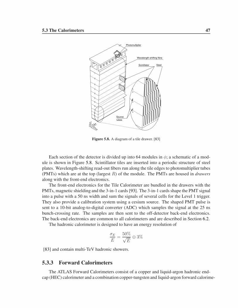
5.3 The Calorimeters 47
Photomultiplier
Wavelength-shifting fibre
Scintillator Steel
Source
tubes
Figure 5.8. A diagram of a tile drawer. [83]
Each section of the detector is divided up into 64 modules in φ; a schematic of a mod-
ule is shown in Figure 5.8. Scintillator tiles are inserted into a periodic structure of steel
plates. Wavelength-shifting read-out fibers run along the tile edges to photomultiplier tubes
(PMTs) which are at the top (largest R) of the module. The PMTs are housed in drawers
along with the front-end electronics.
The front-end electronics for the Tile Calorimeter are bundled in the drawers with the
PMTs, magnetic shielding and the 3-in-1 cards [93]. The 3-in-1 cards shape the PMT signal
into a pulse with a 50 ns width and sum the signals of several cells for the Level 1 trigger.
They also provide a calibration system using a cesium source. The shaped PMT pulse is
sent to a 10-bit analog-to-digital converter (ADC) which samples the signal at the 25 ns
bunch-crossing rate. The samples are then sent to the off-detector back-end electronics.
The back-end electronics are common to all calorimeters and are described in Section 6.2.
The hadronic calorimeter is designed to have an energy resolution of
σE
E=
50%√E
⊕ 3%
[83] and contain multi-TeV hadronic showers.
5.3.3 Forward Calorimeters
The ATLAS Forward Calorimeters consist of a copper and liquid-argon hadronic end-
cap (HEC) calorimeter and a combination copper-tungsten and liquid-argon forward calorime-

5.4 The Muon Spectrometer 48
ter (FCAL). The HEC covers 1.5 < |η| < 3.2 and the FCAL covers 3.1 < |η| < 4.9 and
they are both housed in the same cyrostat as the electromagnetic endcap calorimeters. The
arrangement of the calorimeters is shown in Figure 5.9(a). The design of these detectors
differs from the previously mentioned calorimeters because they need to withstand the high
flux of particles in the forward direction.
The HEC is conceptually similar to the liquid argon calorimeter described above. Scin-
tillator would not withstand the radiation damage it would accrue at small radii to the
beam-line, therefore liquid argon is used instead. The copper takes the place of the lead
absorbers and the detector has a flat plate design, perpendicular to the beam-line, instead
of the accordion structure.
��������������������������������������������
��������������������������������������������
����������
������
������
�����
�����
������������������������������������������������������������������������������������������������������������������������������������������������������������������������������������������������������������������������������������������������������������������������������������������������������������������������������������������������������������������������������������������������������������������������������������������������������������������������������������������������������������������������������������������������������������������������������������������������������������������������������������������������������������������������������������������������������������������������������������������������������������������������������������������������������������������������������������������������������������������������������������������������������������������������������������������������������������������������������������������������������������������������������������������������������������������������������������������������������������������������������������������������������������������
������������������������������������������������������������������������������������������������������������������������������������������������������������������������������������������������������������������������������������������������������������������������������������������������������������������������������������������������������������������������������������������������������������������������������������������������������������������������������������������������������������������������������������������������������������������������������������������������������������������������������������������������������������������������������������������������������������������������������������������������������������������������������������������������������������������������������������������������������������������������������������������������������������������������������������������������������������������������������������������������������������������������������������������������������������������������������������������������������������������������������������������������������������������
450 550500400350 600 650
60
50
40
30
20
10
0
R (
cm)
z (cm)
EMEC
HEC(back)
Pump
FCal 1 FCal 2 FCal 3
(EM) (Had) (Had)
(front)HEC
Moderator shielding shie
ldin
g plu
g
LA
r C
alor
imet
er
(a)
R
LAr gap
Beam-pipe
Warmwall
Super-insulation
Coldwall
(b)
Figure 5.9. (a): Layout of the forward calorimeters. (b): cross-sectional sketch of the FCAL showing the
electrode structure as well as the Moliere radius, RM [83].
The FCAL was designed to provide both electromagnetic and hadronic calorimetry in
an intense radiation environment. The electrodes are formed of coaxial copper rods and
tubes with a very small liquid argon gap in between for fast signal extraction. The gap is
maintained by a radiation hard plastic wire wrapped around the tubes. The electrodes are
held in a copper matrix in the first compartment and a tungsten matrix in the second and
third compartments. The matrix is formed by drilling holes into the passive material plates.
A cross-section of the FCAL is sketched in Figure 5.9(b).
5.4 The Muon Spectrometer
The ATLAS Muon System, shown in Figure 5.10, consists of several different track-
ing technologies arranged around a massive superconducting air-core toroid system. The
toroid consists of a barrel and two end-caps providing 1 to 7.5 Tm in bending power. AT-
LAS chose an air-core design to minimize multiple scattering of the muons so that 10%

5.4 The Muon Spectrometer 49
momentum resolution could be achieved at 1 TeV.
Figure 5.10. A cutaway view of the ATLAS muon system indicating the locations of the various tracking
technologies. [83]
Four different tracking technologies are used. In the barrel, resistive plate chambers
(RPCs) are used for triggering. They consist of parallel resistive plates separated by 2mm
with a potential difference across them. Avalanches are triggered by particles ionizing the
gas (C2H2F4/Iso-C4H10/SF6) in between the plates and are subsequently read-out. These
provide a fast response so that triggering on muons can occur at Level 1. The trade-off
is low position resolution: 10 mm in both z and φ. They are complimented by precision
monitored drift tubes (MDTs) which are built out of pressurized tubes filled with Ar/CO2
gas. Each tube has a coaxial tungsten wire that collects the ionizing charge. The timing
of the signal is used to achieve a z position resolution of 35 µm. In the end-caps, thin gap
chambers (TGCs), which are similar to multi-wire proportional chambers, take the place of
the trigger chambers. Cathode strip chambers (CSCs) provide the precision measurements
in the end-caps. CSCs are multi-wire proportional chambers with segmented cathodes to
improve position resolution.

5.5 The Luminosity Detectors 50
5.5 The Luminosity Detectors
ATLAS uses several detectors for luminosity measurements. In this section only the
detectors relevant to this thesis are discussed.
5.5.1 Minimum Bias Trigger Scintillators
The Minimum Bias Trigger Scintillators (MBTS) are the primary detectors used in this
measurement. They consist of 2 cm thick polystyrene scintillators behind a 3 cm boronated
polyethylene moderator mounted 3.6 m from the interaction point on either side of the
detector. Each side is divided into counters, consisting of an inner (2.09< |η| <2.82,
43 cm < R <88 cm ) and outer( 2.82< |η| <3.84 , 14 cm < R <43 cm ) ring in η and
eight sections in φ, leading to 16 possible measurements per side. In 2010 one of the inner
counters on the C-side (z < 0) was dead, resulting in only 31 total possible measurements.
Each counter is made of two pieces of scintillator glued down the middle. Wavelength
shifting fibers embedded in a machined groove in each half of the scintillator and down the
center of the detector collect the emitted light. The structure of the MBTS detector is shown
in Figure 5.11(a). The wavelength shifting fibers are welded to normal optical fibers which
transmit the signal to the Tile calorimeter PMTs and the readout proceeds exactly as for the
tile calorimeter. The only difference is that the high gain output of the amplifier is sent to
the trigger rather than the low gain, which is the default for tile calorimeter operation.
The MBTS is designed to provide simple and efficient triggering during early data
taking. Each counter’s Tile 3-in-1 card sends a trigger signal. On each side of the detector,
the 16 signals are passed to an amplifier set to minimal gain. There are 2×16 outputs from
the amplifier. One group of 16 is sent to a leading edge (LE) discriminator, the other is
sent to a constant fraction discriminator (CFD). The LE output is then sent to the central
trigger processor which determines how many MBTS counters were over threshold. It then
sets the Level 1 trigger bits L1 MBTS X and L1 MBTS X X, which indicates X MBTS
counters were over threshold or X counters were over threshold on each side, respectively.
The CFD is not currently used. Figure 5.11(b) shows the Level 1 trigger logic.
For the early part of the 2010 running period L1 MBTS 1 was the primary trigger.
As will be shown in Chapter 8.2, it was highly efficient at selecting inelastic interactions.
The MBTS scintillators are not radiation hard, and therefore they will yellow and become
unusable sometime during the 2011-2012 run.
5.5.2 LUCID
LUCID (LUminosity measurement using Cerenkov Integrating Detector2) is ATLAS’s
primary luminosity detector. It is located 17 m from the interaction point and covers 5.5<|η| <5.9. It functions as a relative luminosity detector, with the calibration for absolute
2Perhaps one of the worst reverse-engineered acronyms ever.
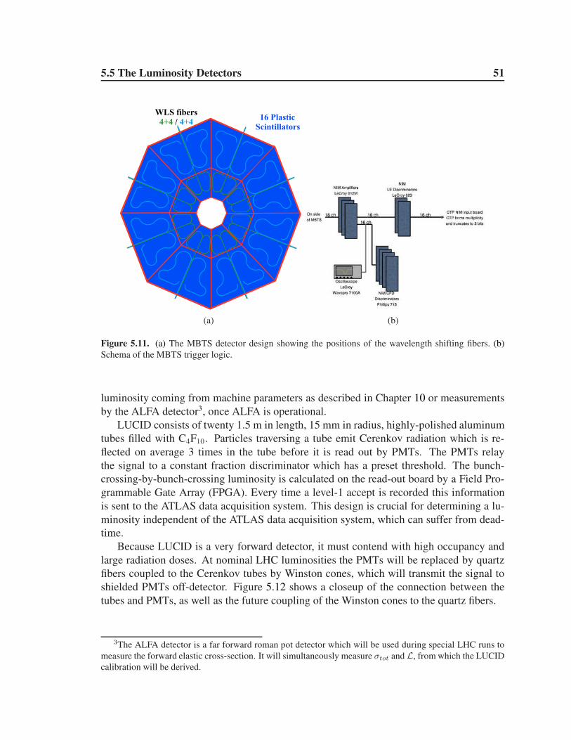
5.5 The Luminosity Detectors 51
WLS fibers16 Plastic
Scintillators4+4 / 4+4
(a) (b)
Figure 5.11. (a) The MBTS detector design showing the positions of the wavelength shifting fibers. (b)
Schema of the MBTS trigger logic.
luminosity coming from machine parameters as described in Chapter 10 or measurements
by the ALFA detector3, once ALFA is operational.
LUCID consists of twenty 1.5 m in length, 15 mm in radius, highly-polished aluminum
tubes filled with C4F10. Particles traversing a tube emit Cerenkov radiation which is re-
flected on average 3 times in the tube before it is read out by PMTs. The PMTs relay
the signal to a constant fraction discriminator which has a preset threshold. The bunch-
crossing-by-bunch-crossing luminosity is calculated on the read-out board by a Field Pro-
grammable Gate Array (FPGA). Every time a level-1 accept is recorded this information
is sent to the ATLAS data acquisition system. This design is crucial for determining a lu-
minosity independent of the ATLAS data acquisition system, which can suffer from dead-
time.
Because LUCID is a very forward detector, it must contend with high occupancy and
large radiation doses. At nominal LHC luminosities the PMTs will be replaced by quartz
fibers coupled to the Cerenkov tubes by Winston cones, which will transmit the signal to
shielded PMTs off-detector. Figure 5.12 shows a closeup of the connection between the
tubes and PMTs, as well as the future coupling of the Winston cones to the quartz fibers.
3The ALFA detector is a far forward roman pot detector which will be used during special LHC runs to
measure the forward elastic cross-section. It will simultaneously measure σtot and L, from which the LUCID
calibration will be derived.

5.5 The Luminosity Detectors 52
15mm
d)
Winstoncone
Fibrebundle
Photomultiplier
Figure 5.12. View of the coupling between the LUCID detector Cerenkov tubes and PMTs, as well as the
future coupling via Winston cones to quartz readout fibers. [83].

53
CHAPTER 6
Event Reconstruction
6.1 Track Reconstruction
This Chapter details elements of the ATLAS event reconstruction relevant to this thesis.
Specifically, the track reconstruction and the calorimeter signal processing are described.
This section concerns aspects of event reconstruction which relate to Inner Detector track-
ing. The ATLAS muon system also provides tracking but it is not discussed here.
6.1.1 Reconstruction Algorithms
Inner Detector reconstruction encompasses track, vertex and beam-spot reconstruction.
The process begins with track reconstruction and concludes with primary vertex finding.
Primary vertices are defined as the locations of proton-proton interactions, and there can
be multiple primary vertices in an event if there are multiple proton interactions. The
primary vertices are used to determine the luminous region, or beam-spot, roughly every
two minutes during data-taking. Each of these steps is detailed below.
Track Reconstruction
The objective of charged particle tracking is to reconstruct a charged particle’s tra-
jectory from the energy it deposits in a detector. Because the detector is immersed in a
magnetic field, the particle will take a helical path which will contain information about
the particle’s momentum vector. Any particle path can be represented by the following five
parameters
d0, z0, φ0, cot θ, q/pT (6.1)
modulo distortions due to energy loss and multiple scattering in the detector. The transverse
impact parameter, d0, is the distance of closest approach of the trajectory to the origin of
the detector in the transverse (x − y) plane. The point of closest approach is referred to
as perigee. The longitudinal impact parameter, z0, is the z coordinate of the trajectory at

6.1 Track Reconstruction 54
perigee. φ0 is the angle at perigee of the trajectory in the transverse plane. The polar angle,
θ, is the angle with respect to the z axis made by the trajectory. The final parameter of the
trajectory is the charged inverse of the particle’s transverse momentum. It is given by the
curvature of the track, ρ = Bq/pT, where B is the magnetic field strength, q is the particle
charge and pT is its momentum in the transverse plane1. A sketch of the parameters in the
transverse and longitudinal planes is shown in Figure 6.1. These parameters can also be
expressed with respect to the point of closest approach to the interaction vertex (primary
vertex), or the beam-spot, indicated by the superscript “PV” and “BS”, respectively.
ρ
d0
dPV0
Primary Vertex
φ0
Nominal
Interaction
Pointx
y
A
(a)
z
ρφ
Nominal
Interaction
Point
Primary Vertex
A
z0
θ
zPV0
(b)
Figure 6.1. An illustration of track parameters in the transverse (a) and longitudinal (b) planes expressed
with respect to the origin of the detector and the primary vertex.
The challenges of track reconstruction can be divided into two categories: track-finding
and track-fitting. In the first, detector hits, .e.g. pixel clusters, SCT clusters, or TRT hits,
are associated to form tracks. In the second, the hits are used to determine the parameters
of the charged particle which created the track. The efficiency to find tracks is discussed in
Section 6.1.2, and the parameter resolution is discussed in Section 6.1.3.
The ATLAS tracking suite is named New Tracking (NEWT) [94] and uses a modular,
multi-stage approach to track reconstruction. A Kalman filter [95] is used as the primary
track fitting algorithm. The tracking begins with an inside-out reconstruction algorithm
which starts with hits in the silicon detectors. The inputs to track finding are spacepoints,
consisting of:
• Pixel clusters, which are formed by clustering neighboring hits in the pixel detector.
The local cluster position and radius of the pixel layer are used to determine a single
three-dimensional point.
1Expressed in natural units assuming a uniform magnetic field.

6.1 Track Reconstruction 55
• Double-sided SCT clusters, which are formed by clustering neighboring hit strips
in the SCT detector. Clusters on opposing sides of each double-sided detector layer
are then associated and the stereo position information is used to provide a single
three-dimensional point.
TRT hits, which provide only two dimensional position information, are used in later parts
of the reconstruction.
The first step of reconstruction creates track seeds, which are formed out of three space-
points on separate layers. All possible combinations of hits from the first pixel layer to
the first layer of the SCT are considered. Then the three measurement points are used to
uniquely determine a circle which gives the seed parameters in the transverse plane, assum-
ing a uniform magnetic field an neglecting multiple scattering. A cut on the pT and d0 of the
seeds is applied to reject bad seeds and speed up the reconstruction. Next, the spacepoints
are discarded and the algorithm uses the seed to define a road to search for hits. Practically
this means that single-sided SCT clusters are used in addition to double-sided ones. It then
proceeds to associate clusters to the track seeds. Each time a hit is associated, the fit is
updated to include its information. A simplified model of the ATLAS detector geometry
is used to predict each step of the filtering, taking into account the material crossed by the
particle.
The hit association phase allows for hits to be shared by multiple tracks or creates fake
tracks out of a random assortment of hits, resulting in a significant fraction of poor quality
tracks. In order to clean up the found tracks, ambiguity solving [96] is used to select good
quality tracks. First, the track is refit with a more sophisticated version of the ATLAS
geometry to better estimate material effects. Second, the track is given a score, taking into
account the χ2/Ndof of the fit, the number and quality of hits from each subdetector and
the number of holes2 associated to the track. An iterative procedure is used to reduce the
hit-sharing between tracks by assigning the shared hit to the track with the higher score and
then refitting both tracks and re-evaluating their score. Once the ambiguity solving step is
finished a quality cut is applied and only tracks passing a configurable threshold are kept.
Lastly, the selected tracks are extrapolated to the TRT to define a road from which to attach
TRT hits. Figure 6.2 illustrates the various steps of track finding. The track reconstruction
process reconstructs tracks up to an |η| of 2.5 and a pT as low as 100 MeV.
After the inside-out tracking is run, the unassociated hits are used to do outside-in
tracking, starting with the TRT. The outside-in tracking must be run last so that the pos-
sible combinations do not overwhelm the pattern recognition. TRT drift circles only give
information in two directions: the r− φ plane in the barrel and φ− z plane in the endcaps.
In the r − φ plane tracks with pT of 500 MeV or greater are nearly straight lines over the
length of the TRT detector and in the φ − z plane they are truly straight lines because the
magnetic field does not produce any bending in that plane. A Hough transform [98] is used
to reconstruct tracks. The transform works by mapping each hit in the r − φ (φ− z) plane
2A hole is defined as an instance when a track is extrapolated through a detector layer but no hit is
associated to it.

6.1 Track Reconstruction 56
Transition
Radiation
Tracker
Silicon
Detectors
TRT Extension
Seed
Silicon
Track
Space PointSilicon
Track
Candidate
Nominal
Interaction
Point
Figure 6.2. Schematic of the different stages of track reconstruction. Spacepoints are represented by the
yellow dots and blue lines indicate track seeds. The dashed blue line is a seed which shares a single hit and
the green line illustrates a seed which was rejected prior to hit association. The green dashed line indicates
a track candidate which failed the impact parameter cuts. The red line represents a silicon-only track. The
black line indicates a track including TRT hits. Figure reproduced from [97] with permission of the author.
into the space of straight lines intersecting the point, φ0 − cT(z), where cT(z) is 1/pT (z):
cT(z) = r(z) · cos(φ0) + φ · sin(φ0) (6.2)
If all hits arise from a single line, the lines in the φ0 − cT (z) plane will intersect at a single
φ0, cT (z) value. Practically, the transform fills a histogram in several η bins for each event
and the local maxima indicate the track segments.
Once a track segment is formed, it is used to define a road into the silicon detector. The
algorithm searches for hits not already associated to an inside-out track. The same track
fitting and scoring is performed as in the inside-out case, although with different criteria for
the scoring. This track finding is powerful for finding electrons from photon conversions
and other secondary particles from decays which are displaced a significant distance from
the primary vertex.

6.1 Track Reconstruction 57
Primary Vertex Reconstruction and Beam Spot Determination
After track-finding is completed, the tracks are used to find the primary event vertex.
Immediately after the data is collected, a 36-hr calibration loop is run on a subset of the
data in which the beam-spot is determined using primary vertices found without knowledge
of the beam-spot. Then the bulk reconstruction is run and primary-vertex finding is rerun
with the constraint of the beam-spot position. The following section describes how the
primary-vertices are reconstructed.
The primary-vertex reconstruction [99] is divided into a finding and a fitting phase, as
in the case of the track reconstruction.
The inputs to the primary vertex finding are tracks satisfying
• pT > 100 MeV
• |d0| < 4 mm
• σ(d0) < 5 mm
• σ(z0) < 10 mm
• NSCT ≥ 4 and NSCT +Npix ≥ 6
where σ(d0)(σ(z0)) is the uncertainty on the d0(z0) measurement. These cuts are used to
reduce the fraction of tracks from secondary particles which are considered for the vertex
finding.
An iterative vertex-finding algorithm is used. First, a vertex seed is determined by his-
tograming the z0 of all of the selected tracks. If the beam-spot has already been determined,
the impact parameter with respect to the beam-spot, zBS0 , is used. The seed position and
nearby tracks are passed to an adaptive vertex fitting [100] algorithm which is χ2 based.
Tracks which are incompatible with the vertex are used to find additional primary vertices
in the event. If the beam-spot has already been determined, the beamspot position is used
as an additional constraint in the vertex fit. In the case of multiple primary vertices in an
event, the vertex with the highest Σp2T of the tracks in the event is the vertex associated
with the hard interaction in the event. The vertex-finding efficiency was found to be over
90% efficient for events with at least two tracks with pT > 100 MeV and fully efficient for
events with at least six tracks with pT > 100 MeV [70].
To determine the beam-spot, vertices with at least four tracks are considered. The
position of the vertices are input to an unbinned maximum likelihood fit which extracts the
beam-spot position in x,y, and z, as well as the width in each coordinate, and any tilt of the
luminous region in the x− z and y − z planes. Typical sizes in the transverse planes were
≈ 0.05 mm and ≈ 40mm in the longitudinal plane in the early 2010 runs.

6.1 Track Reconstruction 58
6.1.2 Tracking Efficiency
The charged particle tracking efficiency is dependent upon many factors such as the
particle type, momentum and the amount of material a particle traverses. Muons, which
have small interaction cross-sections in the 1 GeV to 1 TeV range, have very high track-
ing efficiency. Conversely, pions and protons interact strongly and therefore have lower
tracking efficiency. The amount of material traversed by a particle determines the prob-
ability of having a nuclear interaction, which reduces the tracking efficiency. Electrons
are even more difficult to reconstruct because bremstralung changes the momentum mid-
flight. Lower momentum particles suffer from higher interaction rates and more multiple-
scattering, making track-finding difficult. This section discusses the absolute tracking effi-
ciency as well as studies of the relative efficiency of the silicon based tracking with respect
to the TRT tracking.
Absolute Tracking Efficiency
The absolute tracking efficiency of all particle species can only be determined through
Monte Carlo simulation studies. Generally the efficiency can be described by
ǫ(η, pT, ...) =NTrkMatch(η, pT, ...)
Ngen(η, pT, ...)(6.3)
Where Ngen(η, pT, ...) is the number of generated charged particles as a function of the
η, pT, and any other variables, and NTrkMatch(η, pT, ...) is the subset of those generated
particles which are matched to a track. There are also fake tracks, which are reconstructed
tracks not matched to any generated particles. The definition of a track match is dependent
on the criteria used to do the matching. For example, generated particles can be matched
to tracks by requiring that there be a track within a cone, ∆R =√
∆η2 + ∆φ2 of the
generated particle at perigee. Alternatively, the Monte Carlo simulation information about
which generated particles produced each hit on the track can be used to assign a probability
that the track was created by a particular generated particle.
The following metric is used to assign the probability a track came from a specific
particle:
prob. =10 ·Ngen
pix + 5 ·NgenSCT +Ngen
TRT
10 ·N recpix + 5 ·N rec
SCT +N recTRT
(6.4)
where Ngendet is the subset of the hits on the reconstructed track, N rec
det , which come from
the generated particle. The pixel hits have a larger weight than the SCT hits because there
are less than half as many pixel hits as SCT hits on track. The same reasoning applies
to explain why the TRT hits have much lower weight. A single track can have matches
to multiple generated particles. Therefore, a cutoff of prob =0.55 is applied to determine
whether a generated particle was matched to a track.

6.1 Track Reconstruction 59
The efficiency is determined as a function of pT and η, although the dependence on
other variables was also examined. Figure 6.3 shows the tracking efficiency as a function
of pT and η, as determined in [70].
η
2 1 0 1 2
trk
ε
0.3
0.4
0.5
0.6
0.7
0.8
0.9ATLAS Simulation
| < 2.5η > 100 MeV, | T
p 2, ≥ chn
= 7 TeVs
MC ND
η
2 1 0 1 2
trk
ε
0.3
0.4
0.5
0.6
0.7
0.8
0.9
(a)
[GeV]T
p1 10
trk
ε
0
0.1
0.2
0.3
0.4
0.5
0.6
0.7
0.8
0.9
1ATLAS Simulation
| < 2.5η > 100 MeV, | T
p 2, ≥ chn
= 7 TeVs
MC ND
[GeV]T
p1 10
trk
ε
0
0.1
0.2
0.3
0.4
0.5
0.6
0.7
0.8
0.9
1
(b)
Figure 6.3. Tracking efficiency as a function of η (a) and pT (b) determined with non-diffractive minimum-
bias Monte Carlo events [70].
In order to validate that the simulation accurately describes the tracking quantities and
to give confidence that the efficiencies are correctly modeled, many distributions were stud-
ied. Figure 6.4 shows the average number of pixel and SCT hits on associated to a track as
a function of η for tracks with 100 < pT < 500. This distribution is very sensitive to how
well the Monte Carlo models the tracking in the data, and excellent agreement is found.
However, in Section 11, track distributions for a diffraction-enhanced subset of events is
examined and the agreement between data and MC simulation is worse than shown here.
Relative Silicon Tracking Efficiency
The absolute tracking efficiency used in early tracking analyses must come from the
Monte Carlo simulation as methods for measuring the absolute efficiency require high
statistics and are only applicable to specific particle species. However, constraints can
be placed on the accuracy with which the simulation describes the tracking efficiency with
data-driven techniques. This section describes a technique for measuring the silicon pattern
recognition efficiency.
The combined tracks used for analysis are built from silicon track seeds. Therefore,
it is important to understand the efficiency for the pattern recognition to create a silicon
track, ǫSi. Standalone TRT tracking, in which tracks are formed with a pattern recognition
algorithm which is independent from the inside-out tracking and uses no information from
the silicon detectors, provides a suitable denominator to measure the silicon pattern recog-
nition efficiency. In this study the standalone TRT Tracks are formed using an algorithm

6.1 Track Reconstruction 60
η
2.5 2 1.5 1 0.5 0 0.5 1 1.5 2 2.5
Nu
mb
er
of
Pix
el h
its p
er
tra
ck
3
3.2
3.4
3.6
3.8
4
4.2
4.4
4.6
MC ND
Data 2010
ATLAS
| < 2.5η 2, | ≥ chn
< 500 MeVT
p100 <
= 7 TeVs
(a)
η
2.5 2 1.5 1 0.5 0 0.5 1 1.5 2 2.5
Nu
mb
er
of
SC
T h
its p
er
tra
ck
7
7.5
8
8.5
9
9.5
10
MC ND
Data 2010
ATLAS
| < 2.5η 2, | ≥ chn
< 500 MeVT
p100 <
= 7 TeVs
(b)
Figure 6.4. Average number of pixel (a) and SCT (b) hits as a function of η, comparing data and non-
diffractive minimum-bias Monte Carlo events [70]. Only tracks with 100 < pT < 500 MeV are used.
developed for the combined test beam (CTB)3 which has been modified to work in a colli-
sion environment. Unfortunately this algorithm only works in the TRT barrel. At the time
of the first LHC collisions, the default Hough transform-based Standalone TRT tracking,
which includes the endcaps, was not sufficiently robust to do this analysis.
Comparisons of the TRT and Silicon tracks cannot determine the absolute efficiency,
but a relative efficiency, ǫrSi, of the silicon tracking with respect to the TRT tracking can
be examined by measuring the fraction of good quality TRT tracks for which a matching
silicon track is found. The relative efficiency is defined as
ǫrSi =Nobs
Si+Trt
NobsTrt
(6.5)
(6.6)
where NTrt is the number of TRT tracks and NSi+Trt is subset of TRT tracks matched
to a silicon track. The definition can be expanded using the following equations:
ǫrSi =Nobs
Si+Trt
NobsTrt
(6.7)
NobsSi+Trt
NobsTrt
=ǫmǫTrtǫSiN
ǫTrtN + fTrtNobsTrt
(6.8)
NobsSi+Trt
NobsTrt
=ǫpmǫ
pTrtǫ
pSiN
p + ǫsmǫsTrtǫ
sSiN
s
ǫpTrtNp + ǫsTrtN
s + fTrtNobsTrt
(6.9)
3The combined test beam refers to a period in 2004 when a slice of the Atlas detector was tested at a
beamline at CERN.

6.1 Track Reconstruction 61
where ǫm is the efficiency of the matching parameter, ǫTrt is the TRT tracking efficiency,
N is the number of charged particles and fTrt is the fake rate for TRT tracks. The efficiency
for primaries and secondaries is denoted by the p or s superscript. Primaries are defined
as tracks coming from from the primary vertex or prompt decays. Secondaries come from
decays of long lived particles, nuclear interactions and electrons from photon conversions.
The physics efficiency of interest is the primary efficiency, ǫpSi, and consequently, cuts are
used to limit the contribution from secondaries and fakes.
In the ideal case without secondaries and fakes, the relative efficiency would simplify
to
ǫrSi =Nobs
Si+Trt
NobsTrt
(6.10)
= ǫmǫSi (6.11)
allowing a measurement of the “true” efficiency, up to the efficiency of the matching pa-
rameter. It will be shown that both ǫrSi and the matching parameter distribution agree well
within uncertainties between data and simulation, giving us confidence that the pattern
recognition efficiency for silicon tracks, ǫSi, is described by the simulation.
This study requires that the TRT tracks are in the TRT barrel and have a d0 < 10mm.
The requirement on d0 is looser than that typically used to select primary tracks to allow
for the broader d0 resolution of the TRT. No requirement is placed on the impact parameter
in the z-direction because no measurement of this quantity is provided in the TRT barrel.
In order to ensure that the tracks are well measured they are required to be formed from at
least 20 TRT hits. No requirements are placed on the silicon tracks matched to the TRT
tracks.
The difference in φ0, the azimuthal angle expressed at perigee, between the TRT track
and the closest silicon track is used as the matching parameter, δφTRT−Si. The δφTRT−Si
distributions for both data and simulation are shown in Figure 6.5. The data and MC agree
well and it is notable that there is not a significant difference in the δφTRT−Si distributions
for the nominal geometry and a Monte Carlo sample with extra material in the detector
description, indicating that the method is largely insensitive to the amount of material in
the detector. The matching cut is chosen to be δφTRT−Si < 0.04 radians. The efficiency of
this cut varies with momentum due to the change in resolution with momentum, but a fixed
cut was chosen for simplicity.
Figure 6.6 and Figure 6.7 show the relative silicon tracking efficiency ǫrSi for both data
and simulation. In general, the data and the nominal MC agree well. When looking at
the efficiency as a function of momentum, as in Figure 6.6, deviations between the data
an MC are significantly less than 0.5%. The efficiency is lowest in the 0.5 GeV bin, at
86%. It reaches a plateau near 1 GeV at 96%. By dividing the MC into its primary and
secondary contributions, it is apparent that the shape of the turn on curve is dictated by the
secondary contribution. The primary contribution is nearly fully efficient by 0.6 GeV. The
relative efficiency is lower for the secondaries partly due to the fact that the secondaries are
significantly displaced from the primary vertex and often times do not leave enough hits to
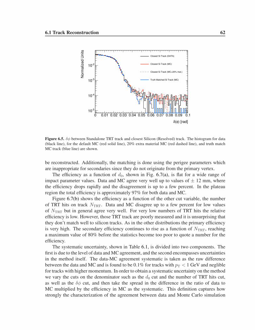
6.1 Track Reconstruction 62
) [rad]φ(δ
0 0.01 0.02 0.03 0.04 0.05 0.06 0.07 0.08 0.09 0.1
No
rma
lize
d U
nits
510
410
310
210
Closest Si Track (DATA)
Closest Si Track (MC)
Closest Si Track (MC+20% mat.)
Truth Matched Si Track (MC)
Figure 6.5. δφ between Standalone TRT track and closest Silicon (Resolved) track. The histogram for data
(black line), for the default MC (red solid line), 20% extra material MC (red dashed line), and truth match
MC track (blue line) are shown.
be reconstructed. Additionally, the matching is done using the perigee parameters which
are inappropriate for secondaries since they do not originate from the primary vertex.
The efficiency as a function of d0, shown in Fig. 6.7(a), is flat for a wide range of
impact parameter values. Data and MC agree very well up to values of ± 12 mm, where
the efficiency drops rapidly and the disagreement is up to a few percent. In the plateau
region the total efficiency is approximately 97% for both data and MC.
Figure 6.7(b) shows the efficiency as a function of the other cut variable, the number
of TRT hits on track NTRT. Data and MC disagree up to a few percent for low values
of NTRT but in general agree very well. For very low numbers of TRT hits the relative
efficiency is low. However, those TRT track are poorly measured and it is unsurprising that
they don’t match well to silicon tracks. As in the other distributions the primary efficiency
is very high. The secondary efficiency continues to rise as a function of NTRT, reaching
a maximum value of 80% before the statistics become too poor to quote a number for the
efficiency.
The systematic uncertainty, shown in Table 6.1, is divided into two components. The
first is due to the level of data and MC agreement, and the second encompasses uncertainties
in the method itself. The data-MC agreement systematic is taken as the raw difference
between the data and MC and is found to be 0.1% for tracks with pT < 1 GeV and neglible
for tracks with higher momentum. In order to obtain a systematic uncertainty on the method
we vary the cuts on the denominator such as the d0 cut and the number of TRT hits cut,
as well as the δφ cut, and then take the spread in the difference in the ratio of data to
MC multiplied by the efficiency in MC as the systematic. This definition captures how
strongly the characterization of the agreement between data and Monte Carlo simulation

6.1 Track Reconstruction 63
[GeV] T
p1
r Si
∈
0.4
0.5
0.6
0.7
0.8
0.9
1
All (DATA)
All (MC)
All (MC+20% mat.)
Primary (MC)
Secondary (MC)
Figure 6.6. Relative efficiency of the Silicon tracking with respect to the TRT tracking as a function of the
pT of the TRT track. Data are in black, nominal Monte Carlo data are in red solid, and 20% extra material
MC in red open circles. Additionally the MC efficiency was divided into primary(blue) and secondary(pink)
contributions.
[mm] 0
d
20 15 10 5 0 5 10 15 20
r Si
∈
0
0.2
0.4
0.6
0.8
1
All (DATA)
All (MC)
All (MC+20% mat.)
Primary (MC)
Secondary (MC)
(a)
TRTN
10 15 20 25 30 35 40 45 50
r Si
∈
0
0.2
0.4
0.6
0.8
1
All (DATA)
All (MC)
All (MC+20% mat.)
Primary (MC)
Secondary (MC)
(b)
Figure 6.7. Relative efficiency of the Silicon tracking with respect to the TRT tracking for d0 and NTRT.
Data are in black, nominal Monte Carlo data are in red solid, and 20% extra material MC in red open circles.
Additional the MC efficiency was divided into primary(blue) and secondary(pink) contributions.
depends upon the specific tracks used to measure the efficiency and the defintion of a match.
As is shown in the table, the variations in the cut values do not significantly effect the
efficiency or the agreement between data and simulation and all variations are at the 0.5%
level or less. In total we measure an uncertainty of a 0.73% on the tracks with 500 MeV <pT <1 GeV and 0.26% for tracks with pT >1 GeV . The uncertainty is higher for the lower
momentum range because the efficiency is changing rapidly in this region, allowing small
discrepancies to have a greater weight than in the plateau region.
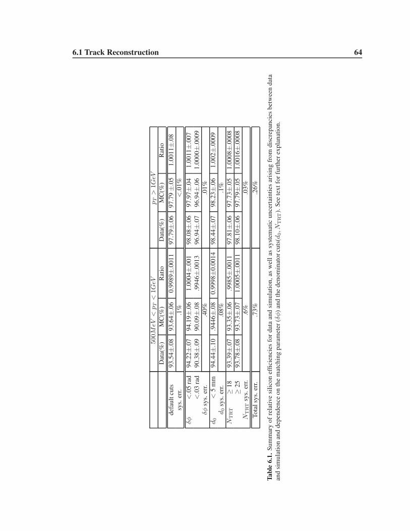
6.1 Track Reconstruction 64
500M
eV<
pT
<1G
eVp
T>
1G
eVD
ata(
%)
MC
(%)
Rat
ioD
ata(
%)
MC
(%)
Rat
io
def
ault
cuts
93
.54±
.08
93
.64±
.06
0.9
98
9±
.00
11
97
.79±
.06
97
.79±
.05
1.0
01
1±
.08
sys.
err.
.1%
<.0
1%
δφ<
.05
rad
94
.22±
.07
94
.19±
.06
1.0
00
4±
.00
19
8.0
8±
.06
97
.97±
.04
1.0
01
1±
.00
7
<.0
3ra
d9
0.3
8±
.09
90
.09±
.08
.99
46±
.00
13
96
.94±
.07
96
.94±
.06
1.0
00
0±
.00
09
δφsy
s.er
r..4
0%
.01
%
d0
<5
mm
94
.44±
.10
.94
46±
.08
0.9
99
8±
0.0
01
49
8.4
4±
.07
98
.23±
.06
1.0
02±
.00
09
d0
sys.
err.
.08
%.1
%
NT
RT
≥1
89
3.3
9±
.07
93
.35±
.06
.99
85±
.00
11
97
.81±
.06
97
.73±
.05
1.0
00
8±
.00
08
≥2
59
3.7
8±
.08
93
.73±
.07
1.0
00
5±
.00
11
98
.10±
.06
97
.79±
.05
1.0
01
6±
.00
08
NT
RT
sys.
err.
.6%
.03
%
To
tal
sys.
err.
.73
%.2
6%
Ta
ble
6.1
.S
um
mar
yo
fre
lati
ve
sili
con
effi
cien
cies
for
dat
aan
dsi
mu
lati
on
,as
wel
las
syst
emat
icu
nce
rtai
nti
esar
isin
gfr
om
dis
crep
anci
esb
etw
een
dat
a
and
sim
ula
tio
nan
dd
epen
den
ceo
nth
em
atch
ing
par
amet
er(δ
φ)
and
the
den
om
inat
or
cuts
(d0,N
TRT
).S
eete
xt
for
furt
her
exp
lan
atio
n.
6.1 Track Reconstruction 65
Tracking Efficiency Systematic Uncertainties
The systematic uncertainties on the tracking efficiency arise from several sources which
are listed below.
• Material: The ability of the Monte Carlo simulation to reproduce the true tracking
efficiency crucially depends on the accuracy of the material modeling in the simula-
tion. The agreement was studied using many methods. One method examined the
reconstructed K0S invariant mass from charged pion decays as a function of the posi-
tion in the detector. A complimentary method looked at the length of tracks which is
sensitive to the nuclear interaction modeling. Additional methods included looking
at the width of hit residuals for low momentum tracks and looking at the efficiency
for a track reconstructed with the pixel detector to be reconstructed in the SCT. The
last method was particularly powerful for assessing the material budget in the for-
ward regions of the detector. It was determined that the material is known to within
10% in the central region of the detector and up to 30% in the highest η regions of
the tracker [70]. This leads to a ± 2 − 15 % uncertainty on the tracking efficiency,
depending on the η and pT of the track.
• Seed Resolution: The tracking resolution effects the tracking efficiency at low mo-
mentum because mismeasured tracks with momentum greater than 100 MeV will
either fall below the minimum track momentum cut of 100 MeV or tracks with lower
momentum will migrate into the track sample. This leads to a ±5% uncertainty be-
tween 100 and 150 MeV.
• Track Selection: The agreement between data and MC on the track selection effi-
ciency was determined by varying the track selection requirements and comparing
the data and MC agreement. This leads to a flat ±1% uncertainty.
6.1.3 Track Resolution
The tracking resolution is a measure of how well the track reconstruction reproduces
the parameters of the particle which created it. At low momenta, the track resolution is
degraded by multiple-scattering. At high momenta, the resolution is driven by how well
the detector is aligned.
Prior to first LHC collisions, the ATLAS inner detector took data with a cosmic ray
trigger with the solenoid on and off. The solenoid-on data provided a unique opportunity to
measure the tracking resolution in-situ with muons. The resolution was measured directly
by splitting the tracks, which pass through both the top and bottom halves of the detector,
into an upper and lower track. The difference of the measured track parameters of the upper
and lower tracks were related to the tracking resolution via the following
δv = vup − vlow (6.12)
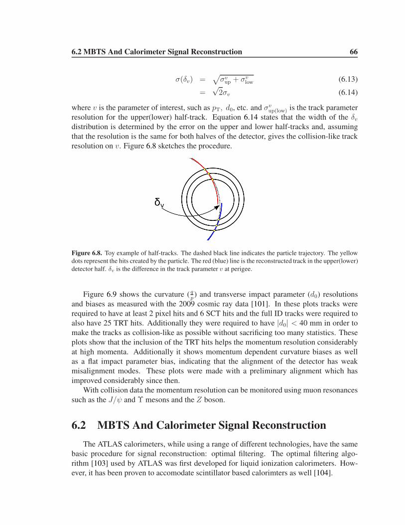
6.2 MBTS And Calorimeter Signal Reconstruction 66
σ(δv) =√
σvup + σv
low (6.13)
=√
2σv (6.14)
where v is the parameter of interest, such as pT, d0, etc. and σvup(low) is the track parameter
resolution for the upper(lower) half-track. Equation 6.14 states that the width of the δvdistribution is determined by the error on the upper and lower half-tracks and, assuming
that the resolution is the same for both halves of the detector, gives the collision-like track
resolution on v. Figure 6.8 sketches the procedure.
Figure 6.8. Toy example of half-tracks. The dashed black line indicates the particle trajectory. The yellow
dots represent the hits created by the particle. The red (blue) line is the reconstructed track in the upper(lower)
detector half. δv is the difference in the track parameter v at perigee.
Figure 6.9 shows the curvature ( qp) and transverse impact parameter (d0) resolutions
and biases as measured with the 2009 cosmic ray data [101]. In these plots tracks were
required to have at least 2 pixel hits and 6 SCT hits and the full ID tracks were required to
also have 25 TRT hits. Additionally they were required to have |d0| < 40 mm in order to
make the tracks as collision-like as possible without sacrificing too many statistics. These
plots show that the inclusion of the TRT hits helps the momentum resolution considerably
at high momenta. Additionally it shows momentum dependent curvature biases as well
as a flat impact parameter bias, indicating that the alignment of the detector has weak
misalignment modes. These plots were made with a preliminary alignment which has
improved considerably since then.
With collision data the momentum resolution can be monitored using muon resonances
such as the J/ψ and Υ mesons and the Z boson.
6.2 MBTS And Calorimeter Signal Reconstruction
The ATLAS calorimeters, while using a range of different technologies, have the same
basic procedure for signal reconstruction: optimal filtering. The optimal filtering algo-
rithm [103] used by ATLAS was first developed for liquid ionization calorimeters. How-
ever, it has been proven to accomodate scintillator based calorimters as well [104].

6.2 MBTS And Calorimeter Signal Reconstruction 67
[GeV]T
p1 10 210
(q/p
)σ
p x
0
0.05
0.1
0.15
0.2
0.25
ATLAS Preliminary Cosmic ’08
Split tracks
Data, full ID
Data, Si only
Simulation, full ID
Split tracks
Data, full ID
Data, Si only
Simulation, full ID
(a)
[GeV]T
p1 10 210
) [m
m]
0(d
σ
0
0.01
0.02
0.03
0.04
0.05
0.06
0.07
0.08
0.09
0.1
ATLAS Preliminary Cosmic ’08
Split tracks
Data, full ID
Data, Si only
Simulation, full ID
Split tracks
Data, full ID
Data, Si only
Simulation, full ID
(b)
[GeV]T
p1 10 210
(q/p
)∆
me
an
p x
−0.1
−0.08
−0.06
−0.04
−0.02
0
0.02
0.04
0.06
0.08
0.1
ATLAS Preliminary Cosmic ’08
Split tracks
Data, full ID
Data, Si only
Simulation, full ID
Split tracks
Data, full ID
Data, Si only
Simulation, full ID
(c)
[GeV]T
p1 10 210
[m
m]
0d
∆m
ea
n
−0.04
−0.03
−0.02
−0.01
0
0.01
0.02
0.03
0.04
ATLAS Preliminary Cosmic ’08
Split tracks
Data, full ID
Data, Si only
Simulation, full ID
Split tracks
Data, full ID
Data, Si only
Simulation, full ID
(d)
Figure 6.9. qp
(a) and d0 (b) resolution versus pT. qp
(c) and d0 (d) resolution bias versus pT. All plots using
cosmic ray data collected in 2009 [102].
The Liquid Argon calorimeters and the Tile Calorimeter share the same basic back-end
electronics to do the signal processing. The MBTS uses Tile PMTs and is fully integrated
into the Tile read-out chain. Read-out drivers (RODs) on the back-end electronics board
contain Digital Signal Processors (DSP) which recieve the samples of the detector signals
from the front-end electronics. The shape of the signal and the number of samplings vary
depending on the detector, but the procedure for fitting for the total charge or energy col-
lected and time of arrival of the signal are the same. This fitting is done by the DSPs for
the Level 2 triggering or in the offline reconstruction.
Each sample can be expressed in terms of the pulse shape function g(t):
Si = p+ Ag(ti + τ) + ni (6.15)
where p is the pedestal, A is the amplitude of the signal, τ is the phase of the signal rela-
tive to the pulse shape function and ni is the noise. If the pulse shape function and noise
are known, then A, τ and p can be determined using a taylor expansion the above equa-
6.2 MBTS And Calorimeter Signal Reconstruction 68
tion [104]:
A =n∑
i=1
aiSi; Aτ =∑n
i=1 biSi; p =n∑
i=1
ciSi (6.16)
where ai, bi, ci are constants which are precalculated for each channel and stored on the
ROD DSPs or in the offline reconstruction database. Knowing A and τ gives the charge
deposited in the detector as well as the time of arrival of the signal. The fit results are
then used for Level 2 trigger decisions. Figure 6.10 shows a toy model of a signal and
samplings. The quality of the fit is also computed and is determined by
χ2 =
n∑
i=1
|(Si − p) −Agi| (6.17)
taking the absolute value is used online instead of squaring each term to reduce compuation
time in the DSPs.
The optimal filtering procedure is performed again during the offline reconstruction,
resulting in a more precise determination of the charge and time of the signal. Figure 6.11
shows the difference in the A- and C-side MBTS signal times for the offline and online
algorithms in collision data [105]. Proton interactions from colliding beams have a ∆t of
0, whereas beam-gas and beam-halo are at ± 25ns. The largest difference in the online
and offline determinations are for the beam-gas and beam-halo events, which are signifi-
cantly out-of-time. The peaks at ± 75ns in the offline are artificial. The differences in the
background peak positions between the online and offline methods are due to biases in the
online signal reconstruction.
The following sections detail the specifics of the Liquid Argon and Tile signals.
6.2.1 Liquid Argon Calorimeters
The Liquid Argon calorimeter signal consists of ionization charge collected by elec-
trodes in the accordian structure. The signal has a very short rise-time and is followed by
a linear decay, but it is shaped by the front end electronics into a bipolar distribution. The
shaped signal as measured with cosmic rays is shown in Figure 6.12(a). The liquid argon
signal is slow, lasting approximately 450 ns. Although sampling every 25 ns is possible,
during normal data-taking only five samples are read-out.
6.2.2 Tile Calorimeter and the MBTS
The Tile Calorimeter signal output are scintillation pulses from PMTs which are shaped
by the analog 3-in-1 card. Figure 6.12(b) shows the analog signal response after shaping in
the high and low gain channels as determined from pion test beams. The shaping stretches
the signals so that the samplings can be made at reasonable intervals. They are sampled

6.2 MBTS And Calorimeter Signal Reconstruction 69
time [ns]25 75 100-75 -25-100 0
Si
(a)
time [ns]25 75 100-75 -25-100 0
Si
τ
(b)
Figure 6.10. Toy representation of a PMT pulse in the black line, the yellow dots represent the sampling
points. (a) represents an in-time pulse, (b) represents a pulse with phase τ .
seven times by the digitizer, as described in Section 5.3.2. The MBTS uses Tile PMTs
and the full Tile readout chain. Therefore, the signals are very similar. Typical charges
collected under the 2010 running conditions by the MBTS are 0.7 pC for a single particle.
The MBTS offline performance is studied in detail in Chapter 8.

6.2 MBTS And Calorimeter Signal Reconstruction 70
mbts time difference AC [ns]
100 80 60 40 20 0 20 40 60 80 100
1
10
210
310
410
510
610online
offlineATLAS Preliminary
Figure 6.11. Difference in timing measurements between the A and C-sides of the MBTS for the online and
offline algorithms in 7 TeV collision data. The differences in the background peak positions are due to biases
in the online signal reconstruction [105].
time (ns)0 100 200 300 400 500 600 700 800
AD
C C
ounts
-400
-200
0
200
400
600
800
1000
1200
1400
-0.04-0.0200.020.04
PS LAYER EM BARREL
2008 ATLAS cosmic muons
ATLAS Preliminary
Prediction
Data
(Data-Prediction)/Max(Data)
Graph
Graph
Graph
(a)
Time [ns]60 40 20 0 20 40 60 80 100 120
a.u
.
0
0.2
0.4
0.6
0.8
1 Low gain
High gain
(b)
Figure 6.12. (a): Liquid argon pulse shape with the data (red points) and prediction(blue points) for cosmic
ray muons. The green points indicate the fractional difference between the data and prediction. (b): Tile
PMT signal shapes determined from pion testbeams for the low gain (solid line) and high gain (dashed line)
channels [106].
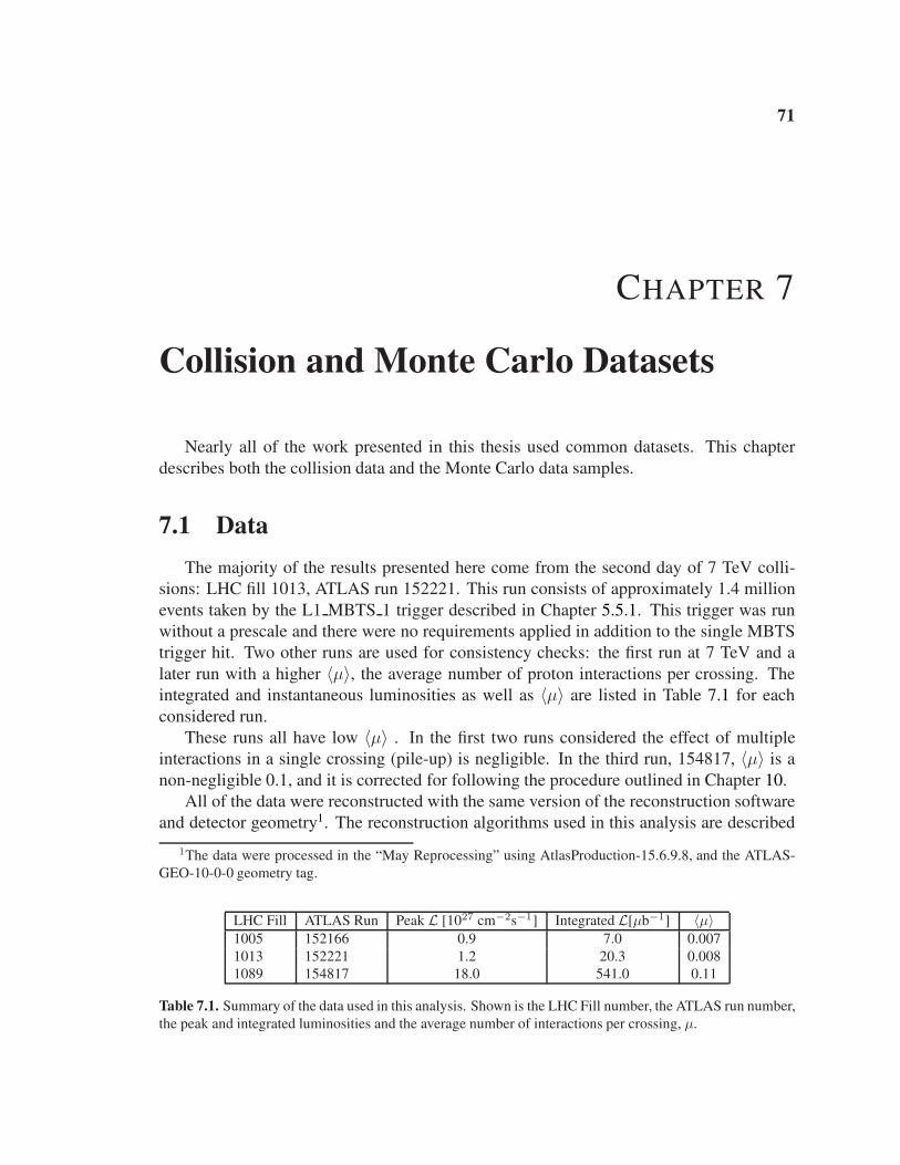
71
CHAPTER 7
Collision and Monte Carlo Datasets
Nearly all of the work presented in this thesis used common datasets. This chapter
describes both the collision data and the Monte Carlo data samples.
7.1 Data
The majority of the results presented here come from the second day of 7 TeV colli-
sions: LHC fill 1013, ATLAS run 152221. This run consists of approximately 1.4 million
events taken by the L1 MBTS 1 trigger described in Chapter 5.5.1. This trigger was run
without a prescale and there were no requirements applied in addition to the single MBTS
trigger hit. Two other runs are used for consistency checks: the first run at 7 TeV and a
later run with a higher 〈µ〉, the average number of proton interactions per crossing. The
integrated and instantaneous luminosities as well as 〈µ〉 are listed in Table 7.1 for each
considered run.
These runs all have low 〈µ〉 . In the first two runs considered the effect of multiple
interactions in a single crossing (pile-up) is negligible. In the third run, 154817, 〈µ〉 is a
non-negligible 0.1, and it is corrected for following the procedure outlined in Chapter 10.
All of the data were reconstructed with the same version of the reconstruction software
and detector geometry1. The reconstruction algorithms used in this analysis are described
1The data were processed in the “May Reprocessing” using AtlasProduction-15.6.9.8, and the ATLAS-
GEO-10-0-0 geometry tag.
LHC Fill ATLAS Run Peak L [1027 cm−2s−1] Integrated L[µb−1] 〈µ〉1005 152166 0.9 7.0 0.007
1013 152221 1.2 20.3 0.008
1089 154817 18.0 541.0 0.11
Table 7.1. Summary of the data used in this analysis. Shown is the LHC Fill number, the ATLAS run number,
the peak and integrated luminosities and the average number of interactions per crossing, µ.
7.2 Monte Carlo Models 72
in Chapter 6.
7.2 Monte Carlo Models
Three primary Monte Carlo simulations are used: PYTHIA 6, PYTHIA 8 and PHOJET.
The details of the physics modeling behind these generators is described in Chapter 2.6.
Several million events were generated for each of the ND, SD, DD and CD (where appli-
cable) processes for each generator. In this document generator-, hadron-, particle- and
truth-level distributions refer to quantities calculated or determined from the four-vectors
of particles produced by the Monte Carlo generators. The term Fully simulated-events
refers to generated events which were passed through the detector simulation [107]. The
detector simulation uses a description of the detector geometry and material implemented
in Geant4 [108] to simulate the interactions of the generated particles with the detector. The
events are then passed through the same software chain as the data. Because the beam-spot
longitudinal width is different in the MC than in the data, the MC events are weighted to
the data beam-spot distribution.
In addition to the three generators mentioned above, a fourth fully simulated sample
is considered to understand the effect of variations in the detector simulation. To obtain
the samples, generated events from the PYTHIA 6 sample were passed through the detector
simulation with a different version of the detector geometry. The events were reconstructed
with the default version of the geometry description, thereby mimicking the effects of hav-
ing an inaccurate material description. The description used2 has a 20% increase in the
radiation length of the Pixel and SCT services. Figure 7.1 compares the total radiation
length of the nominal geometry with the geometry used for the extra material sample and
the “best guess” of the material distribution3 which was determined after the samples were
fully simulated.
When considering alternate models of the diffractive mass spectrum, PYTHIA 8 is used
to generate events according to the alternate spectrum. Then, either the truth information
from those events is used or the fully simulated PYTHIA 8 events are re-weighted to the
truth spectrum. Table 7.2 lists the models considered for the cross-section measurement
Unless otherwise indicated, the PYTHIA relative cross-sections are used to combine the
SD, DD, and ND process for all models except PHOJET.
2ATLAS-GEO-10-00-043ATLAS-GEO-16-00-00

7.2 Monte Carlo Models 73
Figure 7.1. The material distribution in radiation lengths of the inner detector comparing the nominal geome-
try (Geo-10-00-00) with the geometry used for the extra material sample (Geo-10-00-04) and the “best guess”
of the material distribution (Geo-16-00-00) which was determined after the samples were fully simulated.
Generator Cross-section Model Full Sim. ?
PHOJET Engel yes
PYTHIA 6 Schuler-Sjostrand yes
PYTHIA 8 Schuler-Sjostrand yes
Donnachie and Landshoff ǫ = 0.085 α′
= 0.25 GeV−2 no
ǫ = 0.06 α′
= 0.25 GeV−2 no
ǫ = 0.10 α′
= 0.25 GeV−2 no
ǫ = 0.085 α′
= 0.10 GeV−2 no
ǫ = 0.085 α′
= 0.40 GeV−2 no
Bruni and Ingelman no
Berger and Streng no
Table 7.2. Summary of the models used in this analysis. The table indicates the generator was used for the
modeling of exclusive properties, the cross-section model and whether or not fully simulated were available.

74
CHAPTER 8
MBTS Detector Response and Efficiency
Measurements
The validity of the work presented in this thesis depends crucially on the understand-
ing of the MBTS detectors. In particular, the determination of the agreement between the
data and Monte Carlo simulation on the MBTS performance is one of the most critical
experimental aspects of the work. Additionally, the simulation must accurately describe
the material between the interaction point and the MBTS detector because it determines
what fraction of the particles interact before reaching the MBTS. This chapter comprehen-
sively examines the MBTS performance with a particular emphasis on the offline charge
reconstruction and additionally constrains the agreement of the data and simulation on the
material budget in the forward region of the detector. First, the offline noise profiles are de-
termined. Next the trigger efficiency is determined. A data-driven approach to measuring
the MBTS counter offline efficiency follows and the Monte Carlo simulation is tuned to re-
produce the observed efficiency. Lastly, the agreement between the ability of the simulation
to reproduce the material in the ATLAS detector in the MBTS acceptance is assessed.
8.1 Noise Profiles
The noise signal in the MBTS is generated by dark current in the PMTs as well as by
intrinsic noise in the read out electronics which are shared with the Tile Calorimeter. It is
typically well described by a double Gaussian centered at 0 pC. The noise was measured
in the empty LHC bunches using events triggered by the zero bias trigger. The zero bias
trigger randomly selects 25 ns window bunch-crossings with no LHC beam, therefore no
particle signals, apart from exceedingly rare cosmic rays, are expected to contaminate this
sample.
The noise distribution was plotted for each counter in Figure 8.1. All of the coun-
ters have similar noise profiles, and only a few counters have hits greater than ± 0.12 pC.
Counters A5, A14 and C9 have slightly wider distributions. Counter A6 has one hit above

8.1 Noise Profiles 75
Outer A−Side Charge [pC]
0.2 0.1 0 0.1 0.2410
310
210
110
1Counter 8
Counter 9
Counter 10
Counter 11
Counter 12
Counter 13
Counter 14
Counter 15
(a)
Inner A−Side Charge [pC]
0.2 0.1 0 0.1 0.2510
410
310
210
110
1Counter 0
Counter 1
Counter 2
Counter 3
Counter 4
Counter 5
Counter 6
Counter 7
(b)
Outer C−Side Charge [pC]
0.2 0.1 0 0.1 0.2410
310
210
110
1Counter 8
Counter 9
Counter 10
Counter 11
Counter 12
Counter 13
Counter 14
Counter 15
(c)
Inner C−Side Charge [pC]
0.2 0.1 0 0.1 0.2
310
210
110
1Counter 1
Counter 2
Counter 3
Counter 4
Counter 5
Counter 6
Counter 7
(d)
Figure 8.1. MBTS noise distribution measured in empty bunches for all counters on the A-side outer (a) and
inner (b) ring and on the C-side outer (c) and inner (d) ring.
0.2 pC which could be from cosmic rays or “afterglow”, a background described in Chap-
ter 9. Overall, the noise is contained to less than 0.14 pC to the 10−4 level at the time this
data was taken. The noise distribution is expected to widen as the counters accrue radiation
damage. When fit with a double Gaussian, the typical model of the Tile Calorimeter read
out electronics noise, the primary Gaussians have widths of 0.02 pC, while the secondary
widths are generally slightly larger. However, the amplitudes of the second Gaussians are
generally quite small, therefore a single Gaussian is an adequate description of the noise
profile.
In the version of the detector simulation used for the Monte Carlo data processing in
this document, the noise in the MBTS was artificially set to zero. Because new samples
were unavailable at the time of this work, the noise was emulated in the simulation via an
ad hoc smearing to all MBTS signals of a 0.02 pC width Gaussian centered at 0 pC.

8.2 Trigger Efficiency 76
8.2 Trigger Efficiency
The MBTS detector is primarily used by the ATLAS experiment for its highly effi-
cient triggering on inelastic interactions. Its trigger capabilities are described in detail in
Chapter 5.5.1.
In order to measure the trigger efficiency with respect to the offline event selection
requirements, a reference trigger is used. The inelastic cross-section measurement counts
the number of events with at least two offline MBTS hits, where a hit is defined as a counter
with a charge greater that 0.15 pC. To measure the trigger efficiency with respect to that
selection a purely random trigger is used as the reference. It randomly selects bunch-
crossings when both beams are passing through ATLAS. Events from recorded by this
trigger with at least two MBTS offline hits over threshold form the denominator of the
efficiency measurement. The numerator is given by the subset of those event which also
have the L1 MBTS 1 trigger bit set.
cellN
0.5 1 1.5 2 2.5 3 3.5 4 4.5
Eff. w
.r.t O
fflin
e
0.75
0.8
0.85
0.9
0.95
1
Random
Lucid
PairedUnpaired Random
Figure 8.2. Trigger efficiency as a
function of the number of MBTS
cells with an offline charge of at least
0.15 pC. Shown are the efficiencies
as determined using events triggered
by the random trigger with (triangle)
and without (closed circle) subtraction
of unpaired bunches, and using events
triggered by the LUCID trigger (open
circle).
The effect of background was studied by subtracting events in the unpaired bunches
passing a trigger which randomly selects bunch-crossings where a single beam is passing
through ATLAS. No statistically significant effect was found. The trigger efficiency is
measured to be 99.98+0.02−0.12%. A second reference trigger which requires at least one hit
in the LUCID detector (5.6 < |η| < 6.0) is used to set the systematic uncertainty. It is
sufficiently independent from the MBTS trigger because there is no overlap in η between
the two detectors. This method yields an efficiency of 99.91%.
Figure 8.2 shows the efficiency as a function of the number of offline hits. Because
of the low interaction rate of less than 0.01 interactions per crossing, the random trigger
is inefficient at selecting inelastic interactions. For this reason, the trigger efficiency mea-
surement is statistics limited.
In addition to the inelastic cross-section measurement, studies of tracks in a diffraction-
enhanced minimum bias sample are also considered in this document. To measure the
trigger efficiency in a sample with tracks, the efficiency of the L1 MBTS 1 trigger was
studied as a function of the number of tracks in the event. For this measurement, the ran-
dom trigger was used at Level 1 and additionally four pixel and four SCT spacepoints were
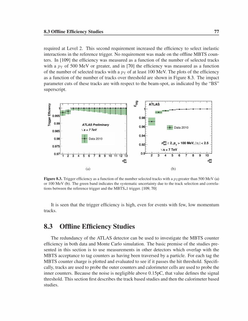
8.3 Offline Efficiency Studies 77
required at Level 2. This second requirement increased the efficiency to select inelastic
interactions in the reference trigger. No requirement was made on the offline MBTS coun-
ters. In [109] the efficiency was measured as a function of the number of selected tracks
with a pT of 500 MeV or greater, and in [70] the efficiency was measured as a function
of the number of selected tracks with a pT of at least 100 MeV. The plots of the efficiency
as a function of the number of tracks over threshold are shown in Figure 8.3. The impact
parameter cuts of these tracks are with respect to the beam-spot, as indicated by the “BS”
superscript.
BSSel
n
1 2 3 4 5 6 7 8 9 10 11 12 13
Trigger
Effic
iency
0.97
0.975
0.98
0.985
0.99
0.995
1
BSSel
n
1 2 3 4 5 6 7 8 9 10 11 12 13
Trigger
Effic
iency
0.97
0.975
0.98
0.985
0.99
0.995
1
Data 2010
ATLAS Preliminary
= 7 TeVs
(a)
BSseln
2 3 4 5 6 7 8 9 10
trig
ε
0.9
0.92
0.94
0.96
0.98
1
BSseln
2 3 4 5 6 7 8 9 10
trig
ε
0.9
0.92
0.94
0.96
0.98
1
Data 2010
ATLAS
| < 2.5η > 100 MeV, | T
p 2, ≥ BSseln
= 7 TeVs
(b)
Figure 8.3. Trigger efficiency as a function of the number selected tracks with a pTgreater than 500 MeV (a)
or 100 MeV (b). The green band indicates the systematic uncertainty due to the track selection and correla-
tions between the reference trigger and the MBTS 1 trigger. [109, 70]
It is seen that the trigger efficiency is high, even for events with few, low momentum
tracks.
8.3 Offline Efficiency Studies
The redundancy of the ATLAS detector can be used to investigate the MBTS counter
efficiency in both data and Monte Carlo simulation. The basic premise of the studies pre-
sented in this section is to use measurements in other detectors which overlap with the
MBTS acceptance to tag counters as having been traversed by a particle. For each tag the
MBTS counter charge is plotted and evaluated to see if it passes the hit threshold. Specifi-
cally, tracks are used to probe the outer counters and calorimeter cells are used to probe the
inner counters. Because the noise is negligible above 0.15pC, that value defines the signal
threshold. This section first describes the track based studies and then the calorimeter based
studies.
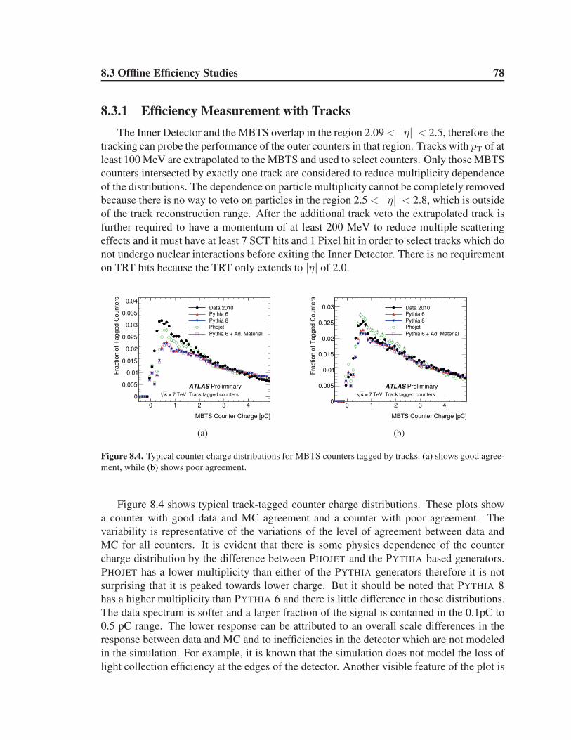
8.3 Offline Efficiency Studies 78
8.3.1 Efficiency Measurement with Tracks
The Inner Detector and the MBTS overlap in the region 2.09< |η| < 2.5, therefore the
tracking can probe the performance of the outer counters in that region. Tracks with pT of at
least 100 MeV are extrapolated to the MBTS and used to select counters. Only those MBTS
counters intersected by exactly one track are considered to reduce multiplicity dependence
of the distributions. The dependence on particle multiplicity cannot be completely removed
because there is no way to veto on particles in the region 2.5 < |η| < 2.8, which is outside
of the track reconstruction range. After the additional track veto the extrapolated track is
further required to have a momentum of at least 200 MeV to reduce multiple scattering
effects and it must have at least 7 SCT hits and 1 Pixel hit in order to select tracks which do
not undergo nuclear interactions before exiting the Inner Detector. There is no requirement
on TRT hits because the TRT only extends to |η| of 2.0.
MBTS Counter Charge [pC]
0 1 2 3 4
Fra
ction o
f T
agged C
ounte
rs
0
0.005
0.01
0.015
0.02
0.025
0.03
0.035
0.04Data 2010Pythia 6
Pythia 8
Phojet
Pythia 6 + Ad. Material
Track tagged counters7 TeV = s
PreliminaryATLAS
(a)
MBTS Counter Charge [pC]
0 1 2 3 4
Fra
ction o
f T
agged C
ounte
rs
0
0.005
0.01
0.015
0.02
0.025
0.03 Data 2010Pythia 6
Pythia 8
Phojet
Pythia 6 + Ad. Material
Track tagged counters7 TeV = s
PreliminaryATLAS
(b)
Figure 8.4. Typical counter charge distributions for MBTS counters tagged by tracks. (a) shows good agree-
ment, while (b) shows poor agreement.
Figure 8.4 shows typical track-tagged counter charge distributions. These plots show
a counter with good data and MC agreement and a counter with poor agreement. The
variability is representative of the variations of the level of agreement between data and
MC for all counters. It is evident that there is some physics dependence of the counter
charge distribution by the difference between PHOJET and the PYTHIA based generators.
PHOJET has a lower multiplicity than either of the PYTHIA generators therefore it is not
surprising that it is peaked towards lower charge. But it should be noted that PYTHIA 8
has a higher multiplicity than PYTHIA 6 and there is little difference in those distributions.
The data spectrum is softer and a larger fraction of the signal is contained in the 0.1pC to
0.5 pC range. The lower response can be attributed to an overall scale differences in the
response between data and MC and to inefficiencies in the detector which are not modeled
in the simulation. For example, it is known that the simulation does not model the loss of
light collection efficiency at the edges of the detector. Another visible feature of the plot is

8.3 Offline Efficiency Studies 79
the small peak at 0 pC. It is primarily due to extrapolation error, i.e. cases where, due to
measurement error, the particle which created the track did not actually intersect the tagged
counter.
Using this distribution three quantities are defined: the fraction of tagged counters with
a charge greater than 0.15 pC, termed the signal fraction (fsig), the fraction of tagged coun-
ters with charge less than 0 pC, termed the zero fraction (fzero), and the efficiency (ǫ) which
is the number of tagged counters with charge greater than 0.15 pC divided by the total num-
ber of tagged counters less twice fzero. The variable fzero is the fraction of counters which
record negative noise. Because the noise is symmetric about 0 pC, twice fzero is the frac-
tion counters recording noise hits. By subtracting twice fzero from the denominator of ǫ,the contribution to the “inefficiency” from cases of extrapolation error is removed.
fsig =NQ>0.15
Ntot
(8.1)
fzero =NQ<0.0
Ntot(8.2)
ǫ =NQ>0.15
Ntot − 2.0 ·NQ<0.0(8.3)
(8.4)
Figure 8.5 shows these quantities for each counter on the A and C side of the detector.
The PYTHIA MCs all have an fsig of approximately 98%, while PHOJET is roughly 0.5%
lower. This can be understood in the context of multiplicity. PHOJET has lower multiplicity,
therefore in the case of extrapolation error, it is less likely that another charged particle
traverses the counter in the region that the tracking does not cover (2.5< |η| <2.8) and
gives an appreciable signal. The data are 1 to 2% lower than the PYTHIA-based Monte
Carlo simulation on average.
fzero is consistent between the data and MC. There are differences of at most 0.4%, but
the overall value agrees well, indicating that the extrapolation error is well modeled in the
MC, as expected. The good agreement suggests that differences in fsig between the data
and the MC are due to inefficiencies in the counters. The plots of the efficiency support
this claim. The PYTHIA-based MC have an average value of 99.4% whereas the data are
closer to 98.5%. Table 8.1 shows fsig, fzero and ǫ averaged over all counters. The C-side
has a slightly higher average efficiency than the A-side in the data.
The excellent angular resolution of the tracks can be used to map the MBTS response
as a function of position in the counter. Figure 8.6 shows fsig, as well as ǫ as a function of φand η. The ǫ versus φ plots varies significantly from counter to counter and also within the
counters. In several instances the efficiency of one half of a counter is substantially different
than the other half. The discrepancy is likely due to differences in the light collection
efficiency of the two pieces of scintillator which comprise each counter. In the fsig plots
both the data and MC exhibit distinct drops in between counters. These drops, which are

8.3 Offline Efficiency Studies 80
fsig fzero ǫData Side A 96.99 ± 0.05 1.32 ± 0.03 98.29 ± 0.04
Data Side C 97.37 ± 0.05 1.41 ± 0.04 98.76 ± 0.04
PYTHIA 6 98.07 ± 0.04 1.38 ± 0.04 99.44 ± 0.02
PYTHIA 8 98.15 ± 0.04 1.30 ± 0.03 99.45 ± 0.02
PHOJET 97.60 ± 0.08 1.71 ± 0.07 99.30 ± 0.04
Extra Material 98.12 ± 0.04 1.35 ± 0.04 99.46 ± 0.02
Table 8.1. Comparison of fsig, fzero, ǫ for data and Monte Carlo simulation for the outer counters as deter-
mined using track tagging.
largely due to extrapolation error, are more pronounced in the data. In the ǫ plots the
MC no longer shows dips between counters, but the effect partially remains in the data.
Near the counter edges the counter light collection efficiency decreases but the losses are
not modeled in the MC, therefore the decrease in efficiency for the data but not the MC
is expected. Additionally there are slight drops in the center of the counters which are
present in the signal fraction in both the data and the MC which are largely absent in the
efficiencies. This effect is not yet understood. There is little dependence of the efficiency
versus η. The data fall off more rapidly at low η than in the MC which is likely due to light
loss at the counter boundaries.
In order to achieve the same efficiencies in the MC as in the data, the MC threshold was
raised until it achieved the data value, separately for each side. The results were consistent
whether fsig or ǫ was used. It was found that the A-side outer counter threshold needed
to be increased to 0.28 pC and the C-side outer counter threshold needed to be raised to
0.26pC.
8.3.2 Efficiency Measurement with the Calorimeters
The calorimeters can be used in the same spirit as the track to probe the counter effi-
ciency. The forward calorimeter (FCAL) spans 3.1 < |η| < 3.8 while the electromagnetic
end-cap (EMEC) covers 2.5 < |η| < 3.2, allowing for studies of the inner counters and
for consistency checks between the outer and inner counters. In this case, exactly one
calorimeter cell above 1 GeV is required to tag a counter. This threshold was chosen to be
above the noise of both the data and the MC.
Examples of counter charge distributions for counters tagged by FCAL and EMEC
cells are shown in figure 8.7. Notably, the distributions from the FCAL tagged counters
shows a significantly lower average charge than those tagged by the EMEC, indicating that
the EMEC selects counters with higher multiplicity than the FCAL because its cell size is
larger.
In both cases the peak at zero charge takes on greater importance than in the track
tagged distributions due to the fact that the calorimeters detects neutral particles while the
MBTS does not. The rate of neutrals, or equivalently, the size of the peak at 0 pC, is

8.3 Offline Efficiency Studies 81
fsig fzero ǫData side A 90.84 ± 0.07 7.02 ± 0.06 97.69 ± 0.04
Data side C 89.97 ± 0.07 7.38 ± 0.06 97.14 ± 0.04
PYTHIA6 90.05 ± 0.07 8.73 ± 0.06 98.66 ± 0.03
PYTHIA8 91.14 ± 0.06 7.69 ± 0.06 98.73 ± 0.03
PHOJET 88.88 ± 0.13 9.74 ± 0.13 98.48 ± 0.05
Extra Material 90.91 ± 0.07 7.96 ± 0.06 98.78 ± 0.03
Table 8.2. Comparison of fsig, fzero, and ǫ for data and Monte Carlo simulation as determined by FCAL-
tagging.
determined by both the particle multiplicity and the material between the interaction point
and the MBTS detector. fzero is examined in detail in Section 8.4.
Efficiencies determined with the FCAL
Figures 8.8 shows fsig, fzero, and ǫ for the FCAL tagged counters. The fsig plots show
variations of 3% among the Monte Carlo simulations and the data appear to agree with
the PYTHIA 8 and the extra material PYTHIA 6 sample. fsig increases with increasing
multiplicity for the Monte Carlo simulations. Also, the extra material sample has a higher
fsig than the nominal PYTHIA 6 sample, indicating that the agreement of the data with the
MCs does not lead to a trivial interpretation.
Figures 8.8(c) and 8.8(d) show the data to have a lower fzero than any of the Monte
Carlo simulations. The interpretation of these results are discussed in the context of the
material description in Section 8.4.
Figures 8.8(e) and 8.8(f) show that the gross dependencies on multiplicity and material
are removed in the ǫ plots. All of the PYTHIA based MCs have the same efficiency, approx-
imately 98.7%, and PHOJET has a slightly lower efficiency, at most 0.5% below PYTHIA.
The data are 1 to 3% less efficient on average. One problematic counter is 4% lower than
the Monte Carlo simulation.
Table 8.2 compares the average fsig, fzero, and ǫ of the Monte Carlo simulation and
of the data on the A-side and C-side separately. There is no difference in the simulation
averages between the A- and C-sides. In order to obtain the same average efficiencies in
the MC as in data the A-side inner counter threshold must be increased to 0.32 pC and the
C-side inner counter threshold must be increased to 0.38 pC.
Efficiencies determined with the EMEC
The EMEC is used as a cross check for both the track and FCAL based methods because
it spans both the inner and outer counters. Its bias towards higher multiplicity makes it less
sensitive to the efficiency of the counters, however it is still useful to confirm the general
trends seen using the other detectors.

8.4 Material 82
Figure 8.9 shows fsig, fzero, and ǫ for EMEC tagged counters. The counter by counter
variations are the same as found with the track and FCAL analyses. In general these distri-
butions show slightly better agreement of the data with the PYTHIA based simulation, but
this can be attributed to the overall higher multiplicity of the sample.
8.4 Material
The amount of material between the interaction point and the MBTS detector plays
a significant role in this analysis, primarily due to its effect on photon conversions. As
explained in Section 8.3, greater amounts of material lead to higher rates of conversions,
which in turn produces a higher charged particle multiplicity in the MBTS acceptance. The
nominal simulation for the MC samples used in this analysis is known to have too little
material in the Pixel services region as well as in other Inner Detector services. The extra
material sample described in Chapter 7 is used for estimation of the material effects. It has a
20% increase in the pixel services radiation length. This is believed to be an underestimate
for 2.2 < |η| < 2.8, an overestimate for 2.8 < |η| < 3.3 and is close to the experiment’s
best guess at the material budget for |η| > 3.3. In the region |η| > 3.3, where material
effects are the most important for the acceptance, the extra material sample has a 15%
increase in total radiation length over the nominal geometry.
In the central region of the detector, |η| < 2.5, the material distribution has been studied
using conversion electrons andK0s → π+π− decays, and is known to better than ±5% up to
|η| < 2.2 and to ±30% for 2.2 < |η| < 2.5 [70]. The large uncertainty in the forward region
is due to lack of statistics as well as known mis-modeling in the geometry description in
that region.
In the forward region of the detector, the material description is assessed using fzero,
which is sensitive to the fraction of converted photons. For two different descriptions of
the material between the interaction point and MBTS detector, the description with more
material will have less events with 0 pC, and consequently a lower fzero, because photons,
primarily from neutral pion decays, are more likely to undergo electron conversion. It
is important to note that fzero is also sensitive to the particle multiplicity. For a given
detector description and two Monte Carlo simulations with different particle multiplicity,
the simulation with higher multiplicity will see less events at 0 pC because it is more likely
that a charged and neutral particle hit the detector at the same time, rather than just a neutral
particle. Both of these effects (higher multiplicity, higher material) lower fzero.
Figures 8.8(c) and 8.8(d) show fzero as measured with the FCAL. PHOJET has the high-
est fzero at nearly 0.1, followed by PYTHIA 6 at 0.09. The PYTHIA 6 extra material sample
has an fzero of roughly 10% less than that of the nominal sample. PYTHIA 8 samples has
an fzero of roughly 0.08. The data value is 0.07 which can be understood in the context of
both the material and multiplicity. The minimum bias measurements [109, 70] indicate that
PYTHIA 8 best reproduces the per-event normalization of the charged particle multiplicity
distribution. Studies for those publications also suggest that the extra material sample is a

8.4 Material 83
better description of the real material budget than the nominal sample in the forward region
of the detector. Therefore it is expected that the data be approximately 0.01 lower than the
PYTHIA 8 fzero value, which is approximately observed. However, if a lower multiplicity,
as predicted by PYTHIA 6, is assumed then 40% more material is needed in the forward
region. The PHOJET Monte Carlo badly under-predicts the average charged particle mul-
tiplicity in inclusive events, therefore it is not used as a baseline from which to assess the
material.

8.4 Material 84
MBTS Counter Number
8 9 10 11 12 13 14 15
sig
f
0.9
0.92
0.94
0.96
0.98
1
Track tagged counters
Data 2010
Pythia 6
Pythia 8
Phojet
Pythia 6 + Ad. Material
(a)
MBTS Counter Number
8 9 10 11 12 13 14 15
sig
f
0.9
0.92
0.94
0.96
0.98
1
Track tagged counters
Data 2010
Pythia 6
Pythia 8
Phojet
Pythia 6 + Ad. Material
(b)
MBTS Counter Number
8 9 10 11 12 13 14 15
zero
f
0
0.01
0.02
0.03
0.04
0.05
0.06
0.07
0.08
0.09
0.1
Track tagged counters
Data 2010
Pythia 6
Pythia 8
Phojet
Pythia 6 + Ad. Material
(c)
MBTS Counter Number
8 9 10 11 12 13 14 15
zero
f
0
0.01
0.02
0.03
0.04
0.05
0.06
0.07
0.08
0.09
0.1
Track tagged counters
Data 2010
Pythia 6
Pythia 8
Phojet
Pythia 6 + Ad. Material
(d)
MBTS Counter Number
8 9 10 11 12 13 14 15
∈M
BT
S C
ounte
r
0.94
0.95
0.96
0.97
0.98
0.99
1
1.01
Data 2010
Pythia 6
Pythia 8
Phojet
Pythia 6 + Ad. Material Track tagged counters
(e)
MBTS Counter Number
8 9 10 11 12 13 14 15
∈M
BT
S C
ounte
r
0.94
0.95
0.96
0.97
0.98
0.99
1
1.01
Data 2010
Pythia 6
Pythia 8
Phojet
Pythia 6 + Ad. Material Track tagged counters
(f)
Figure 8.5. fsig (a,b), fzero (c,d), and ǫ (e,f) for the inner counters tagged by tracks. In all cases A side is on
the left and the C side is on the right.

8.4 Material 85
[rad]φ
3 2 1 0 1 2 3
∈M
BT
S c
ounte
r
0.94
0.95
0.96
0.97
0.98
0.99
1
Data 2010
Pythia 6Track Tagged Counters
= 7TeVs
PreliminaryATLAS
(a)
[rad]φ
3 2 1 0 1 2 3
∈M
BT
S c
ounte
r
0.94
0.95
0.96
0.97
0.98
0.99
1
Data 2010
Pythia 6Track Tagged Counters
= 7TeVs
PreliminaryATLAS
(b)
[rad]φ
3 2 1 0 1 2 3
∈M
BT
S c
ounte
r
0.94
0.95
0.96
0.97
0.98
0.99
1
Data 2010
Pythia 6Track Tagged Counters
= 7TeVs
PreliminaryATLAS
(c)
[rad]φ
3 2 1 0 1 2 3
∈M
BT
S c
ounte
r
0.94
0.95
0.96
0.97
0.98
0.99
1
Data 2010
Pythia 6Track Tagged Counters
= 7TeVs
PreliminaryATLAS
(d)
η
2.1 2.15 2.2 2.25 2.3 2.35 2.4 2.45 2.5
∈M
BT
S c
ounte
r
0.94
0.95
0.96
0.97
0.98
0.99
1
Data 2010
Pythia 6Track Tagged Counters
= 7TeVs
PreliminaryATLAS
(e)
η
2.1 2.15 2.2 2.25 2.3 2.35 2.4 2.45 2.5
∈M
BT
S c
ounte
r
0.94
0.95
0.96
0.97
0.98
0.99
1
Data 2010
Pythia 6Track Tagged Counters
= 7TeVs
PreliminaryATLAS
(f)
Figure 8.6. fsig (a,b), ǫ versus φ (c,d) and ǫ versus η (e,f) determined with tracks of data compared with
PYTHIA 6 Monte Carlo simulation. In all cases A side is on the left, C side is on the right.

8.4 Material 86
MBTS Counter Charge [pC]
0 1 2 3 4
Fra
ction o
f T
agged C
ounte
rs
0
0.01
0.02
0.03
0.04
0.05Data 2010Pythia 6
Pythia 8
Phojet
Pythia 6 + Ad. Material
FCAL tagged counters 7 TeV = s
PreliminaryATLAS
(a)
MBTS Counter Charge [pC]
0 1 2 3 4
Fra
ction o
f T
agged C
ounte
rs
0
0.01
0.02
0.03
0.04
0.05
0.06 Data 2010Pythia 6
Pythia 8
Phojet
Pythia 6 + Ad. Material
FCAL tagged counters 7 TeV = s
PreliminaryATLAS
(b)
MBTS Counter Charge [pC]
0 1 2 3 4
Fra
ction o
f T
agged C
ounte
rs
0
0.002
0.004
0.006
0.008
0.01
0.012
0.014
0.016
0.018
0.02
Data 2010Pythia 6
Pythia 8
Phojet
Pythia 6 + Ad. Material
EMEC tagged counters7 TeV = s
(c)
MBTS Counter Charge [pC]
0 1 2 3 4
Fra
ction o
f T
agged C
ounte
rs
0
0.005
0.01
0.015
0.02
0.025 Data 2010Pythia 6
Pythia 8
Phojet
Pythia 6 + Ad. Material
EMEC tagged counters7 TeV = s
(d)
Figure 8.7. Typical counter charge distributions for MBTS counters tagged by calorimeter cells. FCAL
tagged charged distributions for counter 7 on the A (left) and C (right) sides are on top, EMEC for the same
counters are on bottom.

8.4 Material 87
MBTS Counter Number
0 1 2 3 4 5 6 7
sig
f
0.8
0.82
0.84
0.86
0.88
0.9
0.92
0.94
0.96
0.98
1
FCAL tagged counters
Data 2010
Pythia 6
Pythia 8
Phojet
Pythia 6 + Ad. Material
= 7 TeVs
PreliminaryATLAS
(a)
MBTS Counter Number
1 2 3 4 5 6 7
sig
f
0.8
0.82
0.84
0.86
0.88
0.9
0.92
0.94
0.96
0.98
1
FCAL tagged counters
Data 2010
Pythia 6
Pythia 8
Phojet
Pythia 6 + Ad. Material
= 7 TeVs
PreliminaryATLAS
(b)
MBTS Counter Number
0 1 2 3 4 5 6 7
zero
f
0
0.02
0.04
0.06
0.08
0.1
0.12
FCAL tagged counters
Data 2010
Pythia 6
Pythia 8
Phojet
Pythia 6 + Ad. Material
= 7 TeVs PreliminaryATLAS
(c)
MBTS Counter Number
1 2 3 4 5 6 7
zero
f
0
0.02
0.04
0.06
0.08
0.1
0.12
FCAL tagged counters
Data 2010
Pythia 6
Pythia 8
Phojet
Pythia 6 + Ad. Material
= 7 TeVs PreliminaryATLAS
(d)
MBTS Counter Number
0 1 2 3 4 5 6 7
∈M
BT
S C
ounte
r
0.94
0.95
0.96
0.97
0.98
0.99
1
1.01
Data 2010
Pythia 6
Pythia 8
Phojet
Pythia 6 + Ad. Material FCAL tagged counters
= 7 TeVs PreliminaryATLAS
(e)
MBTS Counter Number
1 2 3 4 5 6 7
∈M
BT
S C
ounte
r
0.94
0.95
0.96
0.97
0.98
0.99
1
1.01
Data 2010
Pythia 6
Pythia 8
Phojet
Pythia 6 + Ad. Material FCAL tagged counters
= 7 TeVs PreliminaryATLAS
(f)
Figure 8.8. Top: fsig, Middle: fzero, Bottom: ǫ for the inner counters tagged by FCAL cells. In all cases A
side is on the left, C side is on the right.

8.4 Material 88
MBTS Counter Number
0 2 4 6 8 10 12 14
sig
f
0.9
0.92
0.94
0.96
0.98
1
EMEC tagged counters
Data 2010
Pythia 6
Pythia 8
Phojet
Pythia 6 + Ad. Material
(a)
MBTS Counter Number
2 4 6 8 10 12 14
sig
f
0.9
0.92
0.94
0.96
0.98
1
EMEC tagged counters
Data 2010
Pythia 6
Pythia 8
Phojet
Pythia 6 + Ad. Material
(b)
MBTS Counter Number
0 2 4 6 8 10 12 14
zero
f
0
0.01
0.02
0.03
0.04
0.05
0.06
0.07
0.08
0.09
0.1
EMEC tagged counters
Data 2010
Pythia 6
Pythia 8
Phojet
Pythia 6 + Ad. Material
(c)
MBTS Counter Number
2 4 6 8 10 12 14
zero
f
0
0.01
0.02
0.03
0.04
0.05
0.06
0.07
0.08
0.09
0.1
EMEC tagged counters
Data 2010
Pythia 6
Pythia 8
Phojet
Pythia 6 + Ad. Material
(d)
MBTS Counter Number
0 2 4 6 8 10 12 14
∈M
BT
S C
ounte
r
0.94
0.95
0.96
0.97
0.98
0.99
1
1.01
Data 2010
Pythia 6
Pythia 8
Phojet
Pythia 6 + Ad. Material EMEC tagged counters
(e)
MBTS Counter Number
2 4 6 8 10 12 14
∈M
BT
S C
ounte
r
0.94
0.95
0.96
0.97
0.98
0.99
1
1.01
Data 2010
Pythia 6
Pythia 8
Phojet
Pythia 6 + Ad. Material EMEC tagged counters
(f)
Figure 8.9. (a),(b): fsig, (c),(d): fzero, (e),(f): ǫ for the inner counters tagged by EMEC cells. In all cases A
side is on the left, C side is on the right.

89
CHAPTER 9
Backgrounds
The measurements in this thesis aim to be as inclusive as possible, therefore there are
no collision backgrounds that need to be modeled as would be the case in an exclusive
measurement, e.g. jets faking electrons in a Z → e+e− measurement. All of the back-
grounds considered here are considered “non-collision” backgrounds and are determined
directly from the data. They fall into two categories: beam-related backgrounds and non
beam-related backgrounds. The beam-related backgrounds include collisions of the beam
with material upstream from the detector or gas in the beam-pipe, as well as the diffuse
radiative background from the interactions of collision remnants with material in the de-
tector called afterglow. Afterglow has two sources, in-time which affects the same bunch-
crossing as when the collision occurred, and out-of-time where the afterglow was produced
by a collision in a different bunch-crossing. Non beam-related backgrounds include noise
and cosmic-rays. Each of these background sources is described in detail in this chapter.
9.1 Beam-Related Backgrounds
Beam-related backgrounds are generally determined from events recorded when only
one beam was passing through ATLAS, termed unpaired bunches. This method is sufficient
for determining the contributions beam-gas, beam-halo and out-of-time afterglow, but is
inadequate for in-time afterglow. Therefore these two categories are treated separately
below.
9.1.1 Beam-Gas, Beam-Halo, Out-of-time Afterglow
Beam-gas, beam-halo, and out-of-time afterglow make up the tradition beam-related
backgrounds. Beam-gas refers to interactions of the beams with gas particles in the beam-
pipe in the interaction region. The ATLAS vacuum is very clean and is able to be evacuated
pressures of 10−11 mbar [110], therefore there are few beam-gas events. However, these
events look very similar to diffractive collision events. Figure 9.1 shows the reconstructed

9.1 Beam-Related Backgrounds 90
vertex position for a run prior to the first 7 TeV collisions when there was a single beam
in the LHC. As it can be seen in the figure, the beam-gas vertex distribution is Gaussian in
the x- and y-coordinates but is flat in the z-distribution. The statistics are poor because the
quality of the ATLAS vacuum leads to few beam-gas events.
(a) (b)
(c) (d)
(e) (f)
Figure 9.1. 1-D and 2-D vertex position distributions from beam-gas events in run 152164.
Beam-halo occurs when particles from the beam interact with material upstream from
the detector, causing a “halo” of particles traversing with the beam, but at large enough
radii to beam-line that they leave hits in the detector. They can be identified by looking
at the difference in the time of hits between the A- and C-sides of the detector. Collision
events have an average time difference of 0 ns while beam-halo events peak around ±25 ns,

9.1 Beam-Related Backgrounds 91
as was shown Figure 6.11.
Both beam-halo and beam-gas events produce hits in the MBTS detectors as well as
tracks in the Inner Detector. As will be shown in Section 11.1.5, the track-based back-
grounds are small and are significantly reduced once a track with pT of 500 MeV is re-
quired.
Afterglow is a poorly understood background which is believed to be due to photons
released by slow neutron capture. The neutrons are produced when collision products
interact with the material in the detector. There is a time-constant associated with the
background of 100s of µs [111], but in high luminosity fills it is still seen hours after the
fill has ended. Figure 9.2(a) the rate of L1 MBTS C triggers are plotted as a function of
the bunch-crossing identifier (BCID) in run 152221. L1 MBTS C consists of the OR of
all individual MBTS counter triggers on the C-side of the detector. There was only one
colliding bunch in ATLAS at BCID 1, which is seen as the large peak in the plot. However,
an exponentially decaying trigger rate is seen for many BCIDs later which is due to the
afterglow. The rate reaches a plateau value of approximately 0.5 Hz. This plateau is due to
noise in the MBTS trigger system as well as long timescale afterglow.
Bunch Id
0 500 1000 1500 2000 2500 3000 3500
Ra
te /
Hz
1
10
MBTS_C Triggers
(a)
Bunch Id
800 1000 1200 1400 1600 1800 2000
Ra
te /
Hz
0.38
0.39
0.4
0.41
0.42
0.43
0.44
0.45
0.46
0.47
0.48
MBTS_C Triggers
(b)
Figure 9.2. Rate of MBTS triggers on the C side of the detector as a function of BCID for run 152221. In
this run the colliding bunch was at BCID=1, and unpaired bunches were present at BCID=892 (from beam
2) and BCID=1786 (from beam 1). The left plots shows all BCID on a log scale, the right zooms in on the
unpaired bunches on a linear scale.
8
Run 152221 had two unpaired bunches traversing ATLAS at BCIDs 1786 (beam 1)
and BCID 892 (beam 2). Figure 9.2(b) is a zoom of the BCID axis in this range. There
are clear peaks of the unpaired bunches over the afterglow background. Therefore the
unpaired bunches are used to estimate the background due to the beam-gas and beam-halo.
Only beam 1 is used because it is less contaminated by afterglow than beam 2. The exact
procedure used for the cross-section analysis is described in detail in Chapter 12.1. For this
thesis, afterglow is a concern only for the MBTS detector.

9.2 Other Backgrounds 92
9.1.2 In-time Afterglow
Figure 9.2(a) suggests that if there is no turn-on behavior, afterglow affects the bunch
in which the collision occurs. This is termed in-time afterglow. The Geant4 simulation
does not model this effect, therefore the data events could have additional MBTS hits not
present in the simulated Monte Carlo events. In-time afterglow is hard to quantify, therefore
a conservative approach is taken. The MBTS has fairly good individual hit time-resolution,
therefore the fraction of late hits, e.g. hits inconsistent with the interaction time, can be
estimated as the afterglow contribution.
Figure 9.3 shows the counter time distribution for events with exactly 1, 2 and 3 coun-
ters above threshold as well as with at least 20 counters above threshold. The Ncounters = 1plots clearly shows the out-of-time afterglow as the component which is flat in time. In the
other plots the unpaired bunches show the beam halo and beam gas events which match
well with features seen in the paired bunches. In the paired bunches the time distribution is
asymmetric, showing a tail at positive times. It is assumed that this tail is attributed solely
to afterglow and, after subtracting off the beam background contribution using the unpaired
bunches, the fraction of hits in the high tail is calculated. The resulting fraction is termed
the ‘hit purity’ and is calculated as
h.p.(Ncounters) = 1 − Ncounters(T > 0) −Ncounters(T < 0)
Ncounters(all T ).
For run 15221 a hit purity of 0.83 is measured for the Ncounters = 2 and Ncounters = 3events. The Ncounters ≥ 20 events have a hit purity of 0.72, most likely due to the fact that
higher multiplicity events will have higher rates of afterglow. The hit purity is a luminosity-
dependent quantity and needs to be determined separately for each run.
9.2 Other Backgrounds
Other backgrounds include spurious hits due to noise as well as cosmic rays. The noise
background can be measured using the BCIDs when there is no beam passing through
ATLAS. As shown in Chapter 8.1, the noise is symmetric about 0 pC, therefore the noise
can also be measured in the paired bunches by looking at the number of counters which
have a charge less than -0.15 pC. Because the threshold is 7σ above the noise, there are no
events recorded.
ATLAS sits 100 m under the earth’s surface, therefore the low energy cosmic ray flux is
significantly attenuated. During cosmic ray data taking the flux through the pixel detector
was measured to be approximately 0.5 Hz. The MBTS horizontal cross-section is consid-
erably smaller, therefore the flux is roughly two orders of magnitude smaller. In the runs
considered there was only one colliding bunch, therefore only one 25ns window every 9 µs
in which a trigger can be recorded. Therefore the cosmic-ray flux is negligible.
In any case, measuring the number of event passing in the unpaired bunches would also
account for the noise and cosmic ray backgrounds, were they significant.

9.2 Other Backgrounds 93
Counter Time [ns]
100 80 60 40 20 0 20 40 60 80 100
10
210
310Paired
Unpaired (Beam 1)
Unpaired (Beam 2)
= 1counterN
(a)
Counter Time [ns]
100 80 60 40 20 0 20 40 60 80 100
1
10
210
310 = 2countersNPaired
Unpaired (Beam 1)
Unpaired (Beam 2)
(b)
Counter Time [ns]
100 80 60 40 20 0 20 40 60 80 100
1
10
210
310 = 3countersN
Paired
Unpaired (Beam 1)
Unpaired (Beam 2)
(c)
Counter Time [ns]
100 80 60 40 20 0 20 40 60 80 100
1
10
210
310
410
510
610 Paired
Unpaired (Beam 1)
Unpaired (Beam 2)
20≥ countersN
(d)
Figure 9.3. MBTS counter time distributions for events with 1,2,3 and ≥20 counters over threshold in run
15221. The colliding bunches are shown by the black histogram and the unpaired bunches in the blue and red
histograms. In all histograms there is one entry per counter above threshold in the event.

94
CHAPTER 10
Luminosity Determination
The determination of the delivered luminosity during the data-taking period used in this
analysis provides the dominant experimental uncertainty. This chapter describes how the
luminosity is measured and how its uncertainties are determined.
10.1 Introduction to Luminosity and Beam Separation Scans
Luminosity is a measure of the total possible interactions per unit area per unit of time
produced by an accelerator [112]. It is the process-independent coefficient relating the
cross-section to observed rate of events
dN
dt= L · σ. (10.1)
Luminosity can be measured in several ways. If σ is well-known, either by previous mea-
surements or by theoretical calculation, and if N can be determined to high accuracy, then
L can be deduced by event-counting. However, the unruly nature of hadron collisions leads
to large uncertainties on σ for all but relatively rare electro-weak processes such as W and
Z production.
Luminosity can also be determined directly from beam parameters through the relation-
ship
L =N1N2fr
Aeff(10.2)
whereN1 andN2 are the number of protons in beam 1 and beam 2, fr is the beam revolution
frequency and Aeff is the effective transverse area in which the two beams overlap [113].
The challenge in this method is to know accurately the number of protons per beam and
the beam sizes, which determines Aeff . For a collider with nb colliding bunches in the ring,
Eqn. 10.2 becomes
L = nbfrn1n2
∫
ρ1(x, y)ρ2(x, y)dxdy (10.3)

10.1 Introduction to Luminosity and Beam Separation Scans 95
where n1,2 are the number of particles per bunch for beam 1 and 2, respectively and
ρ1,2(x, y) is the particle density for each beam in the transverse plane [114]. When the
beam densities are uncorrelated in x and y then Equation 10.3 becomes
L = nbfrn1n2
∫
ρ1(x)ρ2(x)dx
∫
ρ1(y)ρ2(y)dy. (10.4)
∫
ρ1(x)ρ2(x)dx∫
ρ1(y)ρ2(y)dy describes the beam-overlap or luminous region and is equiv-
alent to 1Aeff
in Equation 10.3.
In 1968 Simon van der Meer introduced the concept of beam separation scans, now
called van der Meer (vdM) scans, as a means of measuring the size of the luminous region,
and consequently the luminosity, at CERN’s Intersecting Storage Ring (ISR) [74].
He began with a variable defined by Darriulat and Rubbia [115], the effective beam
height, which is sensitive to the overlap of the beams. It is defined as
beff =
∫
ρ1(x)dx∫
ρ2(x)dx∫
ρ1(x)ρ2(x)dx. (10.5)
which is the charge of the two beams divided by the charge overlap integral. Because the
density profiles can be expressed as a function of unit area times a constant normalization
factor, this is equivalent to the inverse of the overlap fraction of the two beams.
Van der Meer proposed displacing the two beams in x (or y) and measuring the counting
rate as a function of the displacement in order to measure beff . The counting rate, R,
must be proportional to the overlap of the beams and the constant of proportionality, A,
should be independent of the relative beam displacement. Therefore, the counting rate at
displacement h in the x direction is given by
Rx(h) = A
∫
ρ1(x)ρ2(x− h)dx. (10.6)
Van der Meer defined a new variable bnew which is the area under the counting rate integral,
divided by the counting rate at zero displacement. He showed that independently of the
beam shape, this variable is equal to the effective beam height:
bnew =
∫
Rx(h)dh
Rx(0)(10.7)
=
∫ (∫
A · ρ1(x)ρ2(x− h)dx)
dh
A ·∫
ρ1(x)ρ2(x)dx(10.8)
=
∫
(∫
ρ1(x)ρ2(x− h)dh)dx∫
ρ1(x)ρ2(x)dx(10.9)
=
∫
ρ1(x)dx∫
ρ2(x)dx∫
ρ1(x)ρ2(x)dx(10.10)
= beff . (10.11)
(10.12)
10.2 Charged Particle Event Counting and Other Methods 96
Once the beff is known,∫
ρ1(x)ρ2(x)dx is easily determined:
∫
ρ1(x)ρ2(x)dx =
∫
ρ1(x)dx∫
ρ2(x)dx
beff(10.13)
=n1n2
beff(10.14)
=n1n2Rx(0)∫
Rx(h)dh. (10.15)
Before substituting for∫
ρ1(x)ρ2(x)dx in Equation 10.4 the variables Σx,y are defined such
that
Σx,y =1√2π
∫
Rx,y(h)dh
Rx,y(0). (10.16)
Then Equation 10.4 can rewritten as
L =nbfrn1n2
2πΣxΣy
. (10.17)
L now corresponds to the peak instantaneous luminosity which was achieved at zero beam-
displacement.
Knowing L at zero beam-displacement allows for a determination of σ for any given
process:
σvis =dNvis(h = 0)
dt
1
Lh=0. (10.18)
where σvis indicates the visible (i.e. detectable) cross-section for the process of interest.
Therefore dedicated scans are performed to determine σvis for a variety of different pro-
cesses and the resulting cross-sections are used in all other runs to determine the run-by-run
luminosity. The run-by-run luminosity is measured in two-minute intervals, referred to as
’luminosity blocks’.
As will be discussed in Section 10.2, multiple interactions can occur in a single bunch-
crossing. An alternative way of defining the luminosity is
L =µvisnbfr
σvis
. (10.19)
where µvis is the average number of visible interactions of the process of interest [111].
σvis and µvis are related to the total inelastic cross section by σvis = ǫσinel and µvis = ǫµinel
where ǫ is the efficiency to detect an inelastic interaction.
10.2 Charged Particle Event Counting and Other Meth-
ods
The ATLAS experiment uses a number of different detectors and algorithms to deter-
mine the luminosity.

10.2 Charged Particle Event Counting and Other Methods 97
10.2.1 Luminosity Detectors
There is one dedicated luminosity detector, LUCID, which is described in detail in
Section 5.5.2. Other detectors used for online luminosity measurements include the Zero
Degree Calorimeter which sits at ±140m from the interaction point and is sensitive to
forward neutrons and photons, the MBTS, and diamond detectors close to the beam-pipe
at ± 184 cm from the interaction point called beam conditions monitors. There are also
several other detectors used in offline luminosity analyses, including timing information
from the MBTS, timing information for the liquid Argon calorimeters, and charged particle
tracks and primary vertices reconstructed in the Inner Detector. The charged particle track
method will be discussed in detail in Section 10.2.3.
10.2.2 Luminosity Algorithms
Luminosity is currently determined in ATLAS using event counting, although hit count-
ing in specific detectors is also possible. Most online luminosity detectors have two meth-
ods for counting events: OR and AND. OR event counting requires at least one hit in the
detector. AND event counting requires a coincidence of hits in the detector on both sides
of the interaction point. OR has a higher event rate but is more susceptible to backgrounds,
while AND has extremely low background rates. However, the AND algorithm has a
more complicated relationship between the number of observed events and µvis. Offline
methods generally only have one method.
In all cases the luminosity is determined using Equation 10.19. The event counting is
used to determine µvis and σvis is taken from the vdM calibration. Because there can be
more than one interaction per bunch-crossing, a relationship is needed between the number
of observed events and µvis. There are two assumptions made to determine the relation-
ship. First, it is assumed that the average number of interactions per crossing is Poisson
distributed. Second, we assume that the probability for an interaction to be detected is in-
dependent of the presence of a second interaction in the event. This latter assumption is not
strictly true for all of the methods, however it holds for our purposes.
With these two assumptions in hand, the Poisson probability for observing no event
in a given bunch crossing for the OR algorithms is P0(µvis) = e−µvis . It follows that the
probability of observing at least one event is
POR(µvis) =NOR
NBC(10.20)
= 1 − P0(µvis) (10.21)
= 1 − e−µvis . (10.22)
It follows that
µvis = − ln (1 − NOR
NBC). (10.23)

10.2 Charged Particle Event Counting and Other Methods 98
where NOR is the number of events and NBC is the number of bunch-crossings. For an
accelerator with nb number of bunches and a revolution frequency of fr, the number of
events per second, ncorrev , is given by
ncorrev = −nbfr · ln (1 − nev
nbfr
). (10.24)
where nev is the number of observed events per second.
The case of AND algorithms is more complicated. The relationship between the num-
ber of events observed and µvis is not analytically invertible. Therefore, look-up tables are
used to translate from observed events to µvis. The offline algorithms are all treated as ORalgorithms. The ATLAS preferred method is the LUCID OR algorithm.
10.2.3 Charged Particle Event Counting
One of the offline methods used by ATLAS is charged particle event counting. It uses
the number of events with at least one charged particle with pT > 500 MeV and |η| <0.8 to determine the luminosity. This phase space was chosen by the Rate Normalization
Working Group 1 as a phase space accessible to the ALICE, ATLAS and CMS experiments
to facilitate inter-experiment luminosity comparisons.
Practically, the charged particle event rate is determined by counting the number of
events with at least one track in the designated phase space. The track is required to satisfy
the following:
• be associated with a beam-constrained primary vertex with at least two tracks of
pT > 150 MeV.
• |dPV| < 1.5 mm
• |zPV sin θ| < 1.5 mm
• NPix ≤ 0
• NSCT ≥ 5
where dPV and zPV are the transverse and longitudinal distances of closest approach to the
primary vertex, respectively, and NPix(SCT) are the number of Pixel(SCT) hits associated
with the track. Additionally the event must have passed the L1 MBTS 1 trigger.
In order to obtain the number of events with at least one charged particle in the phase
space from the number of events with at least one selected track, event loss due to trigger,
vertex and tracking inefficiency must be corrected for. The corrections are done following
1A working group formed by the LHC Physics Center consisting of members of all four major LHC
experiments and theorists.
10.2 Charged Particle Event Counting and Other Methods 99
the procedure outlined in [116]. Each event is given a weight, wev, to correct for the trigger
and vertex inefficiencies:
wev(nBSsel ) =
1
ǫtrig(nBSsel )
· 1
ǫvtx(nBSsel )
(10.25)
where nBSsel is the number of tracks passing selection requirements when the impact param-
eter cuts are with respect to the beam-spot rather than the primary vertex. ǫtrig(nBSsel ) and
ǫvtx(nBSsel ) are measured in data and found to be high. ǫtrig is nearly 100% for all multiplic-
ities and ǫvtx is 95% for events with nBSsel = 1 and nearly 100% for all others. Both the
trigger and vertex efficiency are 100% for nBSsel ≥ 4.
To correct for loses due to tracking inefficiency, a Monte Carlo simulation-based Bay-
seian unfolding [117] is necessary. First, the ability of the simulation to reproduce the the
tracking efficiency and the fraction of secondary particles passing the track selection is val-
idated extensively as described in [118, 116] and in Section 6.1.2 of this thesis. Then, fully
simulated minimum bias Monte Carlo events2, including mixed ND, SD and DD compo-
nents, are used determine the number of produced primary charged particles, nch, from the
number of selected tracks, nsel. The Monte Carlo events are used to populate a matrix,
Mch,sel with nch as the row position and nsel as the column position. Mch,sel is normalized
such that the total event number does not change, except when nsel > nch which is rare.
The matrix is applied to the nsel distribution in data. The resulting nch distribution is used
to reweight the Mch,sel and this procedure is repeated iteratively until the change between
iterations was less than 1%. Once the nch distribution is obtained, each bin is corrected for
event loss due to tracking inefficiency using the following factor
C(nch) =1
1 − (1 − 〈ǫ(nch)〉)nch(10.26)
where < ǫ(nch) > is the average tracking efficiency in the nch bin. In practice, this correc-
tion is only applied to the first six bins, after which it becomes negligibly small. To obtain
the total number of events with at least one charged particle in the desired phase space,
the corrected nch is integrated. The correction factor from the Ntrk to Nch, where N is the
number of events, is found to be 1.039±0.017. The error includes systematic error on the
tracking efficiency, vertex and trigger efficiencies and on the Monte Carlo-based correction
procedure. The dominant uncertainty is due to the material knowledge uncertainty for the
tracking efficiency. Figure 10.1 shows the nch distribution in a MC closure test.
When determining the charged particle event rate for a particular run, Equation 10.2.2
is used to determine the number of events per second on a lumiblock-by-lumiblock basis.
The charged particle analysis uses the L1 MBTS 1 trigger which, when prescaled, accepts
every s event, where s is the prescale. The error on the number of events passing the
MBTS 1 trigger, s · nMBTS 1, is the Poisson error on s · nMBTS 1 modulo the rounding
error on s. The rounding error is taken into account by adding s/2 to the event count and
2Pythia 6.421 with the ATLAS MC09 Monte Carlo tune was used.

10.2 Charged Particle Event Counting and Other Methods 100
ch
n/d
ev
N d⋅
ev
N1
/
0.05
0.1
0.15
0.2
0.25
0.3
Pythia MinBias AnalysisPythia MinBias Generated
1≥ chn0.8, < |η0.5 GeV, | > T
p
7 TeV = s
ATLAS Version 000
chn
5 10 15 20
Ra
tio
0.9
0.95
1
1.05
1.1
Data UncertaintiesMC Analysis / MC Generated
chn
5 10 15 20
Ra
tio
0.9
0.95
1
1.05
1.1
Figure 10.1. MC closure test of the cor-
rection procedure. The green band indi-
cates the total systematic uncertainties on
the measurement.
s/√
12 to the statistical error. The number of selected events has the additional binomial
uncertainty on the efficiency to select an event given the event passed the trigger. Therefore
the total error on the number of recorded events is given by
σ(nobs) =
√
ǫ · nMBTS 1 · (1 − (1 − 1
s)ǫ) ⊕ ǫ · s√
12(10.27)
Once the µ-correction is applied the error on the corrected number of events is given by
σ(ncorrev ) = s · σ(nobs) ·
nbfr
nbfr − nev(10.28)
Fig. 10.2 shows the resulting raw and corrected rates of events as a function of UTC
time for LHC Fill 1089. The gaps in the run correspond to the second and third van der
Meer scans and times when the ATLAS detector was not taking data.

10.3 Beam Separation Scan Analysis 101
Time (UTC)
05:00:00 11:00:00 17:00:00 23:00:00
Event R
ate
[H
z]
200
300
400
500
600
700
800
900
1000
1100
1≥ chn Correctedµ 1, ≥ chn
LHC Fill 1089 = 7 TeVs
PreliminaryATLAS
> 0.8|η| > 0.5 GeV, T
p
Figure 10.2. Rate of events in LHC
Fill 1089 with at least one charged
primary particle (pT > 0.5 GeV/c,
|η| < 0.8) versus UTC time corrected
(red circles) and uncorrected (black
circles) for multiple interactions.
10.3 Beam Separation Scan Analysis
10.3.1 Scan Descriptions
In 2010 there were five van der Meer scans performed for ATLAS. The first occurred
on April 26th, the second and third on May 9th, and the fourth and fifth on October
1st. Table 10.1 gives parameters of each scan. [111] provides the full details of scans
I through III, [75] details scans IV and V.
In scans I-III there was only one colliding bunch in ATLAS and the beam currents were
relatively low. In scans IV and V there were 6 colliding bunches in ATLAS, which allowed
for a bunch-by-bunch luminosity determination. Additionally, scans IV and V are the only
scans with a crossing angle (200 µrad) and had a significantly higher average number of
interactions per crossing than the previous scans.
For each scan the beams were centered at the nominal interaction point with a three
point mini-scan in both the horizontal (x) and vertical (y) planes. The mini-scans were
performed by using a closed orbit bump, in which the beams are displaced ±1σb by dis-
turbing the beam orbit using pairs of steering dipoles located on either size of the IP. σb
is the nominal transverse beam size. Then the beams were displaced by 3σb in opposite
directions and scanned through ±3σb, leading to a relative displacement of ±6σb. For scan
I this was done first in x and then in y. For scans II and III the beams were taken from
positive to negative nominal separation, followed by a hysteresis cycle where the full ±6σb
separation was run, followed by a scan from negative to positive nominal separation. This
was done first in the x and then in the y direction. In all three of these scans, 27 steps
were taken for scan direction. In IV and V x and y scans were performed sequentially as
in Scan 1, and then repeated to test the reproducibility of the results. In this case, 25 steps
were used. After each scan a re-centering of the beams was performed if necessary. After
the last scan was performed, an x and y scan was performed with the beam offset by 1σ in
the non-scanning direction to test coupling of the beams in x and y.
Figure 10.3 shows the scanning sequence for scans I, II, and III in the horizontal plane.
Figure 10.4 shows the raw and µ-corrected track rates for the same scans. Only data taken

10.3 Beam Separation Scan Analysis 102
vd
MS
can
Iv
dM
Sca
nII
,II
Iv
dM
Sca
nIV
,V
(Ap
ril
26
,2
01
0)
(May
9,2
01
0)
(Oct
ob
er1
,2
01
0)
LH
CF
ill
Nu
mb
er1
05
91
08
91
38
6
Sca
nD
irec
tio
ns
x,y
x,x
,y,y
x,y
,x,y
NS
tep
sp
erP
lan
e2
72
72
5
∆t
per
Ste
p3
0s
30
s2
0s
nb
coll
idin
g1
16
nb
tota
l2
21
9
Np
per
bu
nch
∼0.1·1
011
∼0.2·1
011
∼0.9·1
011
β-f
un
ctio
nat
IP
β⋆
(m)
∼2
∼2
∼3.5
Tra
nsv
erse
sin
gle
bea
msi
ze
σb
(µm
)∼
45
∼45
∼60
Cro
ssin
gan
gle
(µra
d)
00
20
0
L/bu
nch
(µb−
1/s)
4.5·1
0−
31.8·1
0−
20.2
2〈µ〉
0.0
30
.11
1.3
Ta
ble
10
.1.
Su
mm
ary
of
the
mai
nch
arac
teri
stic
so
fth
efi
ve
vdM
scan
sp
erfo
rmed
atth
eA
TL
AS
inte
ract
ion
po
int.
Th
eval
ues
ofL/
bu
nch
and
µar
eg
iven
for
zero
bea
mse
par
atio
n.

10.3 Beam Separation Scan Analysis 103
during specific intervals-of-validity (IOV) were used in the scan analysis. The IOV corre-
spond to the 30 s (scans I-III) or 20 s (scans IV and V) where the beams were not moving
and considered stable.
Time(Hours:Mins)
05:07 05:10 05:14 05:18 05:21 05:25 05:29
Beam
Separa
tion (
mm
)
0.3
0.2
0.1
0
0.1
0.2
0.3
(a)
Time(Hours:Mins)
01:33 01:41 01:49 01:58 02:06 02:14 02:23
Beam
Separa
tion (
mm
)
0.3
0.2
0.1
0
0.1
0.2
0.3
(b)
Figure 10.3. Horizontal beam displacement versus local Geneva time for scan I (a) and scans II
and III (b) [114].
Scan Point
10 20 30 40 50
evts
N
0
1000
2000
3000
4000
5000
6000
7000
(a)
Scan Point
20 40 60 80 100
evts
N
0
5000
10000
15000
20000
25000
(b)
Figure 10.4. Rate of events with at least one track for vdM scan I (a) and Scans II and III (b) as a function
of the scan point. The uncorrected data are in the red open circles, the µ-corrected data are the black points.
10.3.2 Fits for Beam Parameters
For each scan, the event rate was plotted as a function of the beam separation, and
normalized to eliminate beam lifetime effects. The normalization at scan point p is given
by
R(p) =(I1I2)MAX
(I1I2)(p)Rcorr
meas(p) (10.29)

10.3 Beam Separation Scan Analysis 104
where (I1I2)MAX is the maximum product of the beam currents measured during the scan,
(I1I2)(p) is the measured product of the beam currents at scan point p and Rcorrmeas(p) is the
µ-corrected measured event rate at p. R is called the specific rate.
For all algorithms and all scans, the data were fit well by a double Gaussian distribution.
The specific rate as a function of the beam separation was fit to
Rx(x) =Rx(0)√
2π
[
fae−(x−x0)2/2σ2
a
σa+
(1 − fa)e−(x−x0)2/2σ2
b
σb
]
(10.30)
and similarly for the y direction. Substituting this Rx(x) into Equation ?? yields the fol-
lowing expression for Σx
1
Σx=
[
fa
σa+
1 − fa
σb
]
. (10.31)
Figure 10.5 shows the x and y fits for scans I, II, and II for the charged particle event
counting method. Table 10.2 shows the fit results for the same method.
The charged particle method was not used for scans IV and V. Figure 10.6 shows fits
by bunch group for the x scan in scan IV. The details of Scans IV and V fits are found
in [75], what is presented here for the LUCID OR algorithms summarizes the work con-
tained therein.
For each scan the visible cross-section was computed by taking the average of the max-
imum specific rates in x and y and using the following formula
σvis = RMAX 2πΣxΣy
nbfr(n1n2)MAX
(10.32)
where (n1n2)MAX is the maximum product of the number or proton per bunch during the
scan. Table 10.3 has the measured σvis and Lspec for the charged particle method. Averaging
the scans yields a visible cross-section of
σch partvis = 42.7 ± 0.2 mb. (10.33)
The error is purely statistical.
For scans IV and V σvis was determined separately for each BCID and then averaged.
Table 10.4 shows the measured σvis values for those scans with the LUCID OR algorithm.
10.3.3 Uncertainties
Many sources of systematic uncertainty were considered in the vdM scan analysis. This
section summarizes the uncertainty determination detailed in [75].
• Beam Currents The dominant uncertainty is the LHC beam current determination
which is described in detail in [119, 120]. The integrated beam currents are measured

10.3 Beam Separation Scan Analysis 105
Sca
nM
ean
XΣ
XM
ean
YΣ
YR
MA
XX
RM
AX
Yχ
2 X
DO
F
χ2 Y
DO
F
(µm
)(µ
m)
(µm
)(µ
m)
(Hz)
(Hz)
1−
1.6
7±
0.3
47.3±
0.3
−5.6
1±
0.3
556.1±
0.4
253.2±
1.6
249.3±
1.6
0.8
1.4
27.4
2±
0.3
458.5±
0.2
2.2
7±
0.3
662.3±
0.3
869.1±
4.2
841.2±
4.1
1.1
1.1
36.0
3±
0.3
359.3±
0.2
−0.3
2±
0.3
661.5±
0.3
869.6±
4.2
840.6±
4.1
1.1
0.9
Ta
ble
10
.2.
Res
ult
so
fth
efi
tfo
rth
ech
arg
edp
arti
cle
anal
yse
s.T
he
mea
no
fth
eco
nvo
lute
db
eam
wid
thd
istr
ibu
tio
nis
list
edas
mea
np
osi
tio
nX
and
Y,
Σx
and
Σy
are
the
wid
ths
inth
ex
and
yd
irec
tio
ns,
RM
AX
xan
dR
MA
Xy
are
the
max
imu
msp
ecifi
cra
tes
ob
tain
edd
uri
ng
each
scan
,an
dχ
2 X,Y
DO
Far
eth
eχ
2
pro
bab
ilit
ies
div
ided
by
the
nu
mb
ero
fd
egre
eso
ffr
eed
om
of
the
fit.

10.3 Beam Separation Scan Analysis 106
Scan Number σvis Lspec
mb (1029 cm−2s−1)
1 42.61 ± 0.26 6.74 ± 0.052 42.84 ± 0.21 4.91 ± 0.023 42.93 ± 0.21 4.91 ± 0.03
Table 10.3. Measurement of the
visible cross section and peak spe-
cific luminosity for each scan for
the charged particle event counting
method.
LUCID EventOR σvis (mb)
BCID Scan IV Scan V
1 41.76± 0.07 41.68± 0.06501 41.89± 0.07 41.63± 0.06862 41.86± 0.06 41.76± 0.051451 41.78± 0.07 41.74± 0.061651 41.85± 0.07 41.71± 0.072301 41.87± 0.07 41.74± 0.06Average 41.84± 0.03 41.71± 0.02χ2/DOF 0.61 0.66
Table 10.4. Measured σvis val-
ues for the LUCID OR algo-
rithm by BCID. Errors shown
are statistical only. The
χ2/DOF is shown for the 5 de-
grees of freedom in the average
value.
by DC current transformers (DCCT) and the bunch-by-bunch currents are determined
with a relative measurement by the fast beam current transformers(FBCT). The ab-
solute scale of the DCCT varies from fill to fill and has baseline drifts over the course
of a fill. This leads to a 2.7% uncertainty which is uncorrelated between fills. Ad-
ditional sources of current uncertainty arise from knowledge of the baseline offset
as well as the bunch-to-bunch fraction. The uncertainties in these factors decrease
with increasing bunch current, therefore the total beam current uncertainty is 5.6%
for scan I, 4.4% for scans II and III, and 3.1% for scans IV and V.
• Beam Centering In order to achieve the true peak luminosity, the beams must be
centered in the non-scanning plane. The uncertainty was determined by looking at
the difference in the peak position at the beginning and end of the scans. For scans I
through III this is a 2% uncertainty and for scans IV and V this is a 0.04% uncertainty.
• Emittance Growth The beam emittance grows over the course of the fill, changing
the values of Σx and Σy. This should cancel with the corresponding decrease in Rand therefore σvis should be unaffected. This is true for scans IV and V. For scans
I through III, this effect is included in the 3% uncertainty due to non-reproducible
effects.
• Beam-position jitter Jitter in the beam position within a given scan point was de-
termined from the RMS of the beam position distribution within a scan point. This
results in a 0.3% uncertainty for scans IV and V and the 2.7% uncertainty for non-
reproducibility for scans I through III covers this effect.
• Length Scale Calibration The length scale calibration refers to the determination of
the true beam separation at each point in the scan. Dedicated scans were run where
the beams were displaced in the same direction and the beam-spot was determined at

10.3 Beam Separation Scan Analysis 107
each step. The uncertainty on scans I through III is 2% and is largely statistical. The
0.3% uncertainty found for scans IV and V is assumed to be uncorrelated between
the scans.
• Absolute Length Scale of ATLAS detector Because the length scale is determined
using the ATLAS detector, any systematic mismeasurements could lead to a bias in
the length scale. This effect was studied using misaligned Monte Carlo simulation
and found to be at most 0.3%.
• Fit Model A cubic spline fit was used in place of a Gaussian to determine the un-
certainty due to the fit model. The difference in fit results was taken as a systematic
uncertainty. This leads to a 1% uncertainty for scans I through III and 0.2% for
scans IV and V.
• Transverse Correlations Correlations in the beam profiles between the x and yplanes will modify the measured specific luminosity because the density profiles will
no longer factorize. This leads to a 3% uncertainty on scan I, 2% on scans II and III,
and a 0.9% uncertainty on scans IV and V.
• µ-Dependence Scans I, II and III were taken at low µ values, therefore the correc-
tions were small, however a 2% uncertainty was applied based on the agreement
between different algorithms for the value of µ. Scans IV and V had µ values from 0
to 1.3, therefore the agreement between algorithms over that µ range was used to set
an uncertainty of 0.5%.
Table 12.8 summarizes the uncertainties and the level of correlation between scans of the
given error source.
Scan Number I II–III IV–V
Fill Number 1059 1089 1386
Bunch charge product 5.6% 4.4% 3.1% Partially correlated
Beam centering 2% 2% 0.04% Uncorrelated
Emittance growth and
other non-reproducibility 3% 3% 0.5% Uncorrelated
Beam-position jitter – – 0.3% Uncorrelated
Length scale calibration 2% 2% 0.3% Partially Correlated
Absolute ID length scale 0.3% 0.3% 0.3% Correlated
Fit model 1% 1% 0.2% Partially Correlated
Transverse correlations 3% 2% 0.9% Partially Correlated
µ dependence 2% 2% 0.5% Correlated
Total 7.8% 6.8% 3.4%
Table 10.5. Relative systematic uncertainties on the determination of the visible cross section σvis.

10.3 Beam Separation Scan Analysis 108
10.3.4 Results
In order to combine the results from all five scans to determine the luminosity calibra-
tion the statistical and systematic uncertainties, as well as their correlations, were taken
into account. The average value of the LUCID OR σvis is 13.04 ± 0.01 ± 0.44 mb. The χ2
of the combination is 1.6. The combination is dominated by scans IV and V, collectively
contributing 92% of the weight in the fit. The total fractional error is ±3.4%.

10.3 Beam Separation Scan Analysis 109
m]µ x [∆
300 200 100 0 100 200 300
]2
p)
11
[H
z (
10
2 /
N1
Ra
te(T
rk|M
BT
S_
1)
/ N
0
2000
4000
6000
8000
10000
/ ndf 2χ 14.7 / 18
Norm. 7134± 1.099e+06
1
σ 1.092± 43.67
mean 0.307± 1.671
1
fract 0.06601± 0.7834
2
σ 3.813± 67.29
/ ndf 2χ 14.7 / 18
Norm. 7134± 1.099e+06
1
σ 1.092± 43.67
mean 0.307± 1.671
1
fract 0.06601± 0.7834
2
σ 3.813± 67.29
mµRMS: 49.7
mµ 0.3) ±: (47.3 xΣ
m]µ y [∆
300 200 100 0 100 200 300
]2
p)
11
[H
z (
10
2 /
N1
Ra
te(T
rk|M
BT
S_
1)
/ N
0
2000
4000
6000
8000
10000 / ndf 2χ 27.7 / 20
Norm. 7688± 1.289e+06
1
σ 1.844± 45.19
mean 0.3454± 5.613
1
fract 0.0639± 0.4693
2
σ 1.73± 71.22
/ ndf 2χ 27.7 / 20
Norm. 7688± 1.289e+06
1
σ 1.844± 45.19
mean 0.3454± 5.613
1
fract 0.0639± 0.4693
2
σ 1.73± 71.22
mµRMS: 60.4
mµ 0.4) ±: (56.1 yΣ
m]µ x [∆
300 200 100 0 100 200 300
]2
p)
11
[H
z (
10
2 /
N1
Ra
te(T
rk|M
BT
S_
1)
/ N
0
200
400
600
800
1000
1200
1400
/ ndf 2χ 20.38 / 19
Norm. 1167± 2.008e+05
1
σ 0.7506± 56.87
mean 0.3399± 7.418
1
fract 0.03248± 0.929
2
σ 9.412± 94.17
/ ndf 2χ 20.38 / 19
Norm. 1167± 2.008e+05
1
σ 0.7506± 56.87
mean 0.3399± 7.418
1
fract 0.03248± 0.929
2
σ 9.412± 94.17
mµRMS: 60.3
mµ 0.2) ±: (58.5 xΣ
m]µ y [∆
300 200 100 0 100 200 300
]2
p)
11
[H
z (
10
2 /
N1
Ra
te(T
rk|M
BT
S_
1)
/ N
0
200
400
600
800
1000
1200
1400
/ ndf 2χ 20.27 / 19
Norm. 1166± 2.074e+05
1
σ 2.649± 54.7
mean 0.3591± 2.269
1
fract 0.1329± 0.5637
2
σ 3.373± 75.83
/ ndf 2χ 20.27 / 19
Norm. 1166± 2.074e+05
1
σ 2.649± 54.7
mean 0.3591± 2.269
1
fract 0.1329± 0.5637
2
σ 3.373± 75.83
mµRMS: 64.8
mµ 0.3) ±: (62.3 yΣ
m]µ x [∆
300 200 100 0 100 200 300
]2
p)
11
[H
z (
10
2 /
N1
Ra
te(T
rk|M
BT
S_
1)
/ N
0
200
400
600
800
1000
1200
1400
1600 / ndf 2χ 20.43 / 19
Norm. 1151± 2.038e+05
1
σ 0.8496± 58.01
mean 0.3314± 6.033
1
fract 0.03724± 0.9447
2
σ 14± 95.85
/ ndf 2χ 20.43 / 19
Norm. 1151± 2.038e+05
1
σ 0.8496± 58.01
mean 0.3314± 6.033
1
fract 0.03724± 0.9447
2
σ 14± 95.85
mµRMS: 60.7
mµ 0.2) ±: (59.3 xΣ
m]µ y [∆
300 200 100 0 100 200 300
]2
p)
11
[H
z (
10
2 /
N1
Ra
te(T
rk|M
BT
S_
1)
/ N
0
200
400
600
800
1000
1200
1400
/ ndf 2χ 16.61 / 19
Norm. 1197± 2.051e+05
1
σ 3.976± 49.97
mean 0.3608± 0.3209
1
fract 0.1349± 0.3748
2
σ 2.502± 71.37
/ ndf 2χ 16.61 / 19
Norm. 1197± 2.051e+05
1
σ 3.976± 49.97
mean 0.3608± 0.3209
1
fract 0.1349± 0.3748
2
σ 2.502± 71.37
mµRMS: 64.2
mµ 0.3) ±: (61.5 yΣ
Figure 10.5. Fit results for the 1st (top), 2nd (middle) and 3rd (bottom) VdM scan using the charged particle
event counting method.

10.3 Beam Separation Scan Analysis 110
x [mm]∆
0.4 0.3 0.2 0.1 0 0.1 0.2 0.3 0.4
]2
pro
ton
s)
11
(1
01
[B
C2
n 1 /
nV
ISµ
0
0.2
0.4
0.6
0.8
1 LUCID_Event_ORScan IVBCID 1
ATLAS Preliminary
LHC Fill 1386
x [mm]∆
0.4 0.3 0.2 0.1 0 0.1 0.2 0.3 0.4
]2
pro
ton
s)
11
(1
01
[B
C2
n 1 /
nV
ISµ
0
0.2
0.4
0.6
0.8
1 LUCID_Event_ORScan IVBCID 501
ATLAS Preliminary
LHC Fill 1386
x [mm]∆
0.4 0.3 0.2 0.1 0 0.1 0.2 0.3 0.4
]2
pro
ton
s)
11
(1
01
[B
C2
n 1 /
nV
ISµ
0
0.2
0.4
0.6
0.8
1 LUCID_Event_ORScan IVBCID 862
ATLAS Preliminary
LHC Fill 1386
x [mm]∆
0.4 0.3 0.2 0.1 0 0.1 0.2 0.3 0.4
]2
pro
ton
s)
11
(1
01
[B
C2
n 1 /
nV
ISµ
0
0.2
0.4
0.6
0.8
1LUCID_Event_ORScan IVBCID 1451
ATLAS Preliminary
LHC Fill 1386
x [mm]∆
0.4 0.3 0.2 0.1 0 0.1 0.2 0.3 0.4
]2
pro
ton
s)
11
(1
01
[B
C2
n 1 /
nV
ISµ
0
0.2
0.4
0.6
0.8
1 LUCID_Event_ORScan IVBCID 1651
ATLAS Preliminary
LHC Fill 1386
x [mm]∆
0.4 0.3 0.2 0.1 0 0.1 0.2 0.3 0.4
]2
pro
ton
s)
11
(1
01
[B
C2
n 1 /
nV
ISµ
0
0.2
0.4
0.6
0.8
1LUCID_Event_ORScan IVBCID 2301
ATLAS Preliminary
LHC Fill 1386
Figure 10.6. Fit results for the the LUCID OR algorithm for six different bunch groups for Scan IV [75].

111
CHAPTER 11
Comparisons of Monte Carlo Modeling
of Diffractive Events
Before Monte Carlo models are used to assess the acceptance of the cross-section mea-
surement, their ability to reproduce basic kinematic distributions of the data must be veri-
fied. Chapter 2 described the models Monte Carlo generators use to predict multiple parti-
cle production in non-diffractive and diffractive dissociation events. This chapter presents
studies of the agreement between data and the Monte Carlo models on exclusive quan-
tities in diffractive events. First, the ability of the Monte Carlo generators to reproduce
charged particle distributions in a diffraction-enhanced sample is examined. This section
largely summarizes work presented in [121]. Then, the data and Monte Carlo models are
compared in the MBTS acceptance.
11.1 Track-based Studies
Distributions of charged particles are powerful tools for assessing data and Monte Carlo
model agreement because they are sensitive to the properties of single particles. Refer-
ence [70] gives a comprehensive look at the properties of charged particles and events with
at least two charged particles with pT > 100 MeV and |η| < 2.5. This phase space is domi-
nated by non-diffractive events. In order to tune the Monte Carlo parameters related to low
momentum 2 → 2 scattering, charged particle multiplicity, pseudorapidity and momentum
distributions are used. To minimize the effects of the uncertainty in diffractive modeling,
diffractive-suppressed phase spaces are often used. Some experiments attempt to address
this by removing the single-diffractive events from their datasets [122, 123, 124] while AT-
LAS has published additional results in a high-multiplicity, high-momentum phase space
where diffractive events are greatly suppressed [70].
In order to understand how well the generators model exclusive quantities in diffrac-
tive events, this section presents charged particle multiplicity, pseudorapidity and momen-
tum distributions in a phase space which is dominated by diffractive dissocation events.

11.1 Track-based Studies 112
The events are selected by requiring that there be hits on only one of the two sides of the
MBTS detector. As will be shown in Section 11.1.3, this selection results in a diffraction-
dominated sample. Section 11.1.1 outlines the study. The datasets and event and track
selection are described in Section 11.1.2. Section 11.1.4 discusses the agreement between
data and the detector simulation for the tracking and MBTS detectors. Section 11.1.5 re-
views the systematic uncertainties on the measurement, and Section 11.1.6 presents the
comparisons.
11.1.1 Overview of Studies
A sample enhanced in diffractive events is created by selecting events where there is
at least one MBTS hit on exactly one side of the detector (A- or C-side). Only one hit
is required because the additional requirement of a track, which is detailed below, signifi-
cantly reduces the backgrounds for events with just one hit over threshold. This selection
essentially requires the presence of a forward rapidity gap in the event and therefore pref-
erentially selects single-diffractive dissociation events and double-diffractive dissociation
events in which the diffractive mass of one of the proton remnants is too small to be seen
by the MBTS detectors1.
This analysis further requires a track with a transverse momentum of at least 500 MeV
and |η| < 2.5, similar to the selection in [109]. The details of the track selection are given
in Section 11.1.2.
To investigate the event kinematics, the following distributions are plotted:
1
Nev
dNtrk
dη,
1
Nev
1
2πpT
d2Ntrk
dηdpT,
1
Nev
dNev
dntrk,
1
Nev
dNtrk
d∆η(11.1)
whereNev is the number of events with at least one track satisfying the single-sided MBTS
requirements, pT is the transverse momentum, η is the pseudorapidity of the track, ntrk is
the number of selected tracks per event, and Ntrk is the total number of selected tracks in
the data sample. The variable ∆η is the absolute value of the difference in pseudorapidity
between the edge of the MBTS detector that has no hit (ηMBTS) and the track, i.e. ∆η =|ηMBTS −η| where ηMBTS is +2.08 or −2.08 depending on which MBTS side did not have
any hits. Tracks which enter this distribution cannot overlap in η with the MBTS acceptance
of the side of the detecto which did not have any hits, i.e. η > ηMBTS (η < ηMBTS) if
ηMBTS < 0 (ηMBTS > 0).
Unlike the minimum bias analysis measurements cited above, these measurements are
not corrected for detector effects. Corrections for tracking inefficiency and event loss to
obtain charged particle level distributions are beyond the scope of this study. However,
systematic uncertainties reflecting the agreement between data and detector simulation are
1In terms of ξ = M2X/s, ξ must be greater than 5×10⁻⁶ and less than 5×10⁻⁴.In the case of double-
diffraction the lower mass dissociation system must have a mass less than 5×10⁻⁶. The ξ−acceptance is
discussed in more detail in Chapter 12.

11.1 Track-based Studies 113
Run L (µb−1) NEv
152166 7.0 0.5M
152221 20.2 1.4M
Table 11.1.
Luminosity and
number of events
recorded in the stream
physics MinBias.
presented. Therefore, the remaining differences between data and Monte Carlo events are
attributed to differences in physics modeling.
11.1.2 Datasets and Event Selection
Data Sets and MC samples
The data used in this study come from the two ATLAS runs at√s = 7 TeV taken in
late March and early April described in Chapter 7: 152166 and 152221. Only luminosity
blocks where both the Inner Detector and the MBTS detector were functioning properly
are considered. The integrated luminosity is approximately 27 µb−1. Table 11.1 gives the
luminosity and the number of events in the physics MinBias stream, a data stream including
all minimum bias triggers.
The Monte Carlo samples used are the same as those described in Chapter 7. Only the
Schuler-Sojstrand SD and DD differential cross-section models are used for the PYTHIA
8 generators because this study is more sensetive to the charged particle kinematics than
the diffractive mass distribution. The Monte Carlo events were weighted to approximately
reproduce the longitudinal beamspot width observed in data. No reconstructed vertex is
required for this event selection, therefore, an exact weighting cannot be performed.
Event and Track Selection
All events considered in the analysis must pass the L1 MBTS 1 trigger and have hits
on only the A- or the C-side of the MBTS detector (but not both). In addition, at least one
reconstructed track fulfilling the following requirements:
• pT > 500 MeV
• |η| <2.5
• |dBS0 | <1.5 mm
• |z0| < 100 mm
• NPix ≥ 1
• NSCT ≥ 6
is required. This event selection does not require a primary vertex due to the relatively
low vertex finding efficiency for the events of interest. Because they produce few central
charged particles, many diffractive events do not have a reconstructed vertex.

11.1 Track-based Studies 114
Generator ADD1−trk ASD
1−trk AND1−trk
Pythia 6 39.2% 37.0% 97.5%
Pythia 8 50.1% 55.6% 97.3%
Phojet 52.2% 63.7% 95.9%
Table 11.2.
Acceptances for
events to have at
least one track with
pT > 500 MeV
and |η| < 2.5 for
PYTHIA6, PYTHIA8
and PHOJET for
double-diffractive
(DD), single-
diffractive (SD) and
non-diffractive (ND)
events.
Generator DD SD ND
ADDincl−trk ADD
ss−trk ASDincl−trk ASD
ss−trk ANDincl−trk AND
ss−trk
Pythia 6 97.23% 23.89% 97.67% 20.73% 99.9% 0.68%
Pythia 8 99.97% 26.97% 99.97% 22.93% 100.0% 0.13%
Phojet 97.89% 14.22% 97.80% 22.03% 100.0% 0.48%
Table 11.3. Acceptances for events with activity in either side of the MBTS, Aincl−trk, and on only one side
of the MBTS, Ass−trk , for events with at least one track with pT > 500 MeV and |η| < 2.5 for Pythia 6,
Pythia 8 and Phojet for double-diffractive (DD), single-diffractive (SD) and non-diffractive (ND) events.
11.1.3 Acceptance
The acceptances of the track requirement are give in Table 11.2 for the single-dissociation,
double-dissociation, and non-diffractive events for the three MC programs. PYTHIA 8 and
PHOJET both predict that 50% of DD events will have a track, while PYTHIA 6 predicts
only 40%. Similarly, for SD events PYTHIA 6 predicts nearly 20% few events passing than
PYTHIA 8 and 25% less than PHOJET. The gap between PYTHIA 6 and the other genera-
tors is due to is soft diffractive component. The generators predict between 95 and 97% of
ND events pass the track cut.
Table 11.3 gives the acceptances of the MBTS hit requirement for double-diffractive,
single-diffractive and non-diffractive events for PYTHIA6, PYTHIA8 and PHOJET. These
acceptances are with respect to the track requirement. Both the inclusive (at least one hit in
the MBTS detector) and single-sided (at least one hit on exactly one side of the detector)
are shown for comparison purposes. The total acceptance is obtained by multiplying the
numbers from Table 11.3 with those of Table 11.2.
It Table 11.3 the acceptances vary between 14% and 27% for the single-sided require-
ment for diffractive production, while for non-diffractive production the acceptances are
less than 1% for all generators. For the inclusive requirement of any MBTS hit the accep-
tance is > 97% in all cases. The high acceptance value is expected because at least one
central charged particle is ensured by the track requirement. Th generators predict similar
acceptance values for the SD process but differ by nearly a factor two in the DD predictions.

11.1 Track-based Studies 115
11.1.4 Data and Simulation Response Agreement
Before determining the level of agreement between data and Monte Carlo models on
underlying physics distributions, the degree to which the simulation reproduces the re-
sponse of the detector and reconstruction must be assessed. The MBTS performance was
extensively validated in Chapter 8. This section concentrates on the tracking performance
for this event sample.
Chapter 6.1 and [109] already demonstrated that the data and Monte Carlo simulation
agree well for inclusive minimum bias measurements. Because this study has a different
event and track selection, it is necessary to check that the same level of agreement is found.
Figure 11.1 shows a comparison of the transverse and longitudinal impact parameter dis-
tribution between data and PHOJET MC for the single-sided sample.
[mm]BS
0d
1.5 1 0.5 0 0.5 1 1.5
Arb
itra
ry U
nits
0
0.2
0.4
0.6
0.8
1
1.2
1.4
1.6
1.8
2
Data
Phojet MC
(a)
[mm]BS
0d
5 4 3 2 1 0 1 2 3 4 5
Arb
itra
ry U
nits
310
210
110
1Data
Phojet MC
(b)
[mm]0z
150 100 50 0 50 100 150
Arb
itra
ry U
nits
0
0.002
0.004
0.006
0.008
0.01
0.012
0.014
0.016Data
Phojet MC
(c)
[mm]0z
250 200 150 100 50 0 50 100 150 200 250
Arb
itra
ry U
nits
810
710
610
510
410
310
210 Data
Phojet MC
(d)
Figure 11.1. A comparison of transverse (a, b) and longitudinal (c, d) impact parameter distributions for
events passing the single sided event selection. These distributions are shown applying all cuts apart from
that on the quantity shown. The data (markers) are compared to PHOJET (histogram)
The agreement between data and simulation is fairly good for the transverse impact
parameter distribution both in the core and the tails of the distribution. The data z0 distri-
bution is slightly broader than the simulation distribution, indicating that the re-weighting
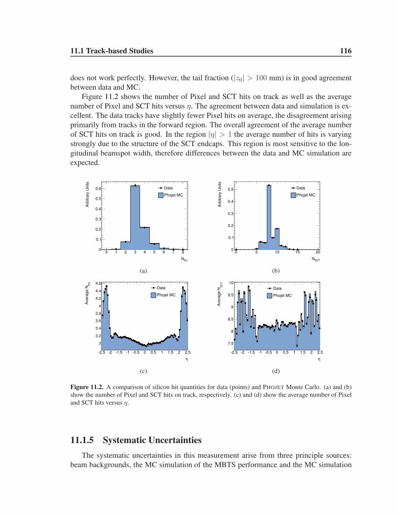
11.1 Track-based Studies 116
does not work perfectly. However, the tail fraction (|z0| > 100 mm) is in good agreement
between data and MC.
Figure 11.2 shows the number of Pixel and SCT hits on track as well as the average
number of Pixel and SCT hits versus η. The agreement between data and simulation is ex-
cellent. The data tracks have slightly fewer Pixel hits on average, the disagreement arising
primarily from tracks in the forward region. The overall agreement of the average number
of SCT hits on track is good. In the region |η| > 1 the average number of hits is varying
strongly due to the structure of the SCT endcaps. This region is most sensitive to the lon-
gitudinal beamspot width, therefore differences between the data and MC simulation are
expected.
PixN
0 1 2 3 4 5 6 7 8
Arb
itra
ry U
nits
0
0.1
0.2
0.3
0.4
0.5
0.6 Data
Phojet MC
(a)
SCTN
0 5 10 15 20
Arb
itra
ry U
nits
0
0.1
0.2
0.3
0.4
0.5 Data
Phojet MC
(b)
η
2.5 2 1.5 1 0.5 0 0.5 1 1.5 2 2.5
Pix
Ave
rag
e N
3
3.2
3.4
3.6
3.8
4
4.2
4.4
4.6Data
Phojet MC
(c)
η
2.5 2 1.5 1 0.5 0 0.5 1 1.5 2 2.5
SC
TA
ve
rag
e N
7.5
8
8.5
9
9.5
10
Data
Phojet MC
(d)
Figure 11.2. A comparison of silicon hit quantities for data (points) and PHOJET Monte Carlo. (a) and (b)
show the number of Pixel and SCT hits on track, respectively. (c) and (d) show the average number of Pixel
and SCT hits versus η.
11.1.5 Systematic Uncertainties
The systematic uncertainties in this measurement arise from three principle sources:
beam backgrounds, the MC simulation of the MBTS performance and the MC simulation

11.1 Track-based Studies 117
of the tracking performance. Each subject is discussed in the following.
Beam Backgrounds
Beam backgrounds are described in Chapter 9. For this study the background is deter-
mined using the single, non-colliding (unpaired) bunches which traverse ATLAS. The two
runs considered contain 41.5k MBTS triggered events in the unpaired bunches, 39.7k of
which have activity on only one side of the MBTS. These numbers can be compared to the
1.4M MBTS triggered events in the paired bunches, 0.2M of which are single-sided. Once
a track fulfilling all the selection cuts is required, there are 52 events passing the MBTS
trigger in the unpaired bunches, 1 of which passes the single-sided selection. Loosening
the track pT requirement to 100 MeV yields 322 MBTS triggered events, 5 of which are
single-sided. The colliding bunches have 1.2M MBTS triggered events with at least one
500 MeV track, with a subset of 5.3k single-sided events. Therefore it is concluded that
the beam background represents less than 0.02% of the number of events selected in the
colliding bunches and is neglected.
MBTS Response
The MBTS response systematic uncertainty was determined prior to the completion
of the studies presented in Chapter 8. Therefore, a conservative method is used to assign
the uncertainty. The threshold for the simulated events was kept at 0.15 pC and the data
threshold was raised to 0.3 pC. Then, the analysis was repeated and the fractional difference
in the resulting distributions (Equation 11.1.1) was taken as the uncertainty. It was assigned
as a symmetric uncertainty, thereby covering the fact that the MC were more efficient than
the data. The main result of the variation is to increase the number of ND events passing
the cut. Intuitively the increase happens because ND events are most likely to have hits
on both sides of the MBTS, and when the threshold is raised, hits can be lost, mimicking
the single-sided selection. The data support this explanation: η distribution becomes more
central and the pT and ntrk spectra become harder due to the larger contamination from ND
events.
Inaccuracies in the modeling of the material between the interaction point and the
MBTS detectors were checked with the extra material PYTHIA 6 sample. Differences
of less than 0.1% were found in the fraction of single-sided events, and therefore material
effects were ignored in the MBTS response systematic uncertainties.
Tracking Performance
The performance of the Inner Detector tracking has been studied extensively in [109,
70]. This analysis applies the same track selection aside from the impact parameter cuts,
which are with respect to the primary event vertex in [109, 70] instead of the beam spot as
in this track selection. Because the difference is small and the distributions are well mod-
eled by simulation, the tracking efficiency uncertainties are taken directly from Ref. [?].
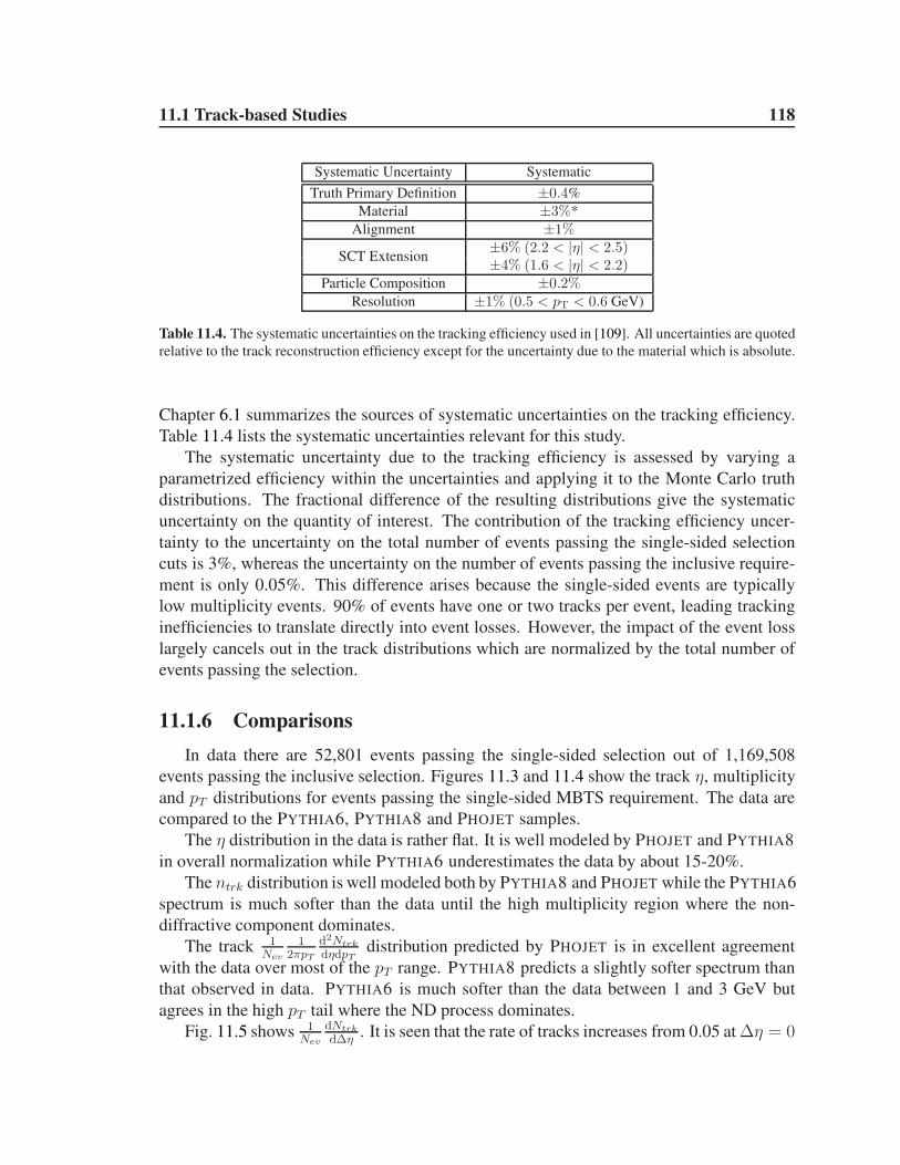
11.1 Track-based Studies 118
Systematic Uncertainty Systematic
Truth Primary Definition ±0.4%
Material ±3%*
Alignment ±1%
SCT Extension±6% (2.2 < |η| < 2.5)±4% (1.6 < |η| < 2.2)
Particle Composition ±0.2%Resolution ±1% (0.5 < pT < 0.6 GeV)
Table 11.4. The systematic uncertainties on the tracking efficiency used in [109]. All uncertainties are quoted
relative to the track reconstruction efficiency except for the uncertainty due to the material which is absolute.
Chapter 6.1 summarizes the sources of systematic uncertainties on the tracking efficiency.
Table 11.4 lists the systematic uncertainties relevant for this study.
The systematic uncertainty due to the tracking efficiency is assessed by varying a
parametrized efficiency within the uncertainties and applying it to the Monte Carlo truth
distributions. The fractional difference of the resulting distributions give the systematic
uncertainty on the quantity of interest. The contribution of the tracking efficiency uncer-
tainty to the uncertainty on the total number of events passing the single-sided selection
cuts is 3%, whereas the uncertainty on the number of events passing the inclusive require-
ment is only 0.05%. This difference arises because the single-sided events are typically
low multiplicity events. 90% of events have one or two tracks per event, leading tracking
inefficiencies to translate directly into event losses. However, the impact of the event loss
largely cancels out in the track distributions which are normalized by the total number of
events passing the selection.
11.1.6 Comparisons
In data there are 52,801 events passing the single-sided selection out of 1,169,508
events passing the inclusive selection. Figures 11.3 and 11.4 show the track η, multiplicity
and pT distributions for events passing the single-sided MBTS requirement. The data are
compared to the PYTHIA6, PYTHIA8 and PHOJET samples.
The η distribution in the data is rather flat. It is well modeled by PHOJET and PYTHIA8
in overall normalization while PYTHIA6 underestimates the data by about 15-20%.
The ntrk distribution is well modeled both by PYTHIA8 and PHOJET while the PYTHIA6
spectrum is much softer than the data until the high multiplicity region where the non-
diffractive component dominates.
The track 1Nev
12πpT
d2Ntrk
dηdpTdistribution predicted by PHOJET is in excellent agreement
with the data over most of the pT range. PYTHIA8 predicts a slightly softer spectrum than
that observed in data. PYTHIA6 is much softer than the data between 1 and 3 GeV but
agrees in the high pT tail where the ND process dominates.
Fig. 11.5 shows 1Nev
dNtrk
d∆η. It is seen that the rate of tracks increases from 0.05 at ∆η = 0
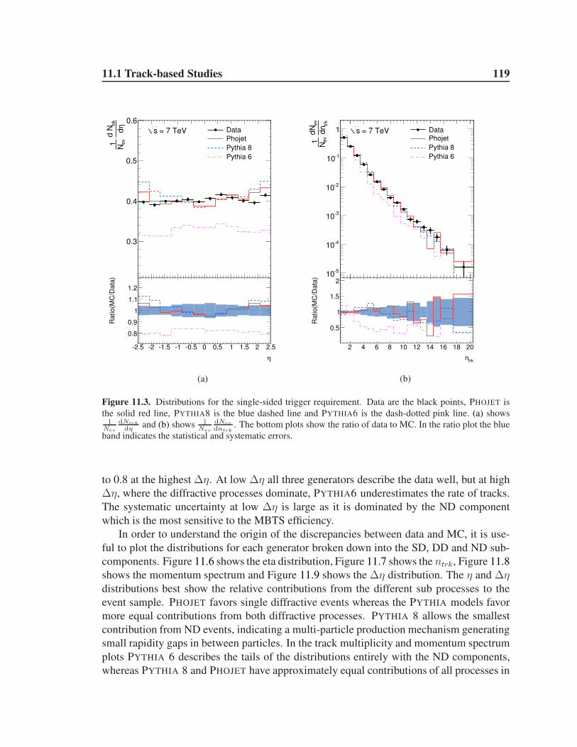
11.1 Track-based Studies 119
ηd
trk
d N
e
vN1
0.3
0.4
0.5
0.6Data
Phojet
Pythia 8
Pythia 6
= 7 TeVs
η
2.5 2 1.5 1 0.5 0 0.5 1 1.5 2 2.5
Ratio(M
C/D
ata
)
0.8
0.9
1
1.1
1.2
(a)
trk
dn
ev
dN
e
vN1
510
410
310
210
110
1 DataPhojet
Pythia 8
Pythia 6
= 7 TeVs
trkn
2 4 6 8 10 12 14 16 18 20
Ratio(M
C/D
ata
)
0.5
1
1.5
2
(b)
Figure 11.3. Distributions for the single-sided trigger requirement. Data are the black points, PHOJET is
the solid red line, PYTHIA8 is the blue dashed line and PYTHIA6 is the dash-dotted pink line. (a) shows1
Nev
dNtrk
dηand (b) shows 1
Nev
dNev
dntrk. The bottom plots show the ratio of data to MC. In the ratio plot the blue
band indicates the statistical and systematic errors.
to 0.8 at the highest ∆η. At low ∆η all three generators describe the data well, but at high
∆η, where the diffractive processes dominate, PYTHIA6 underestimates the rate of tracks.
The systematic uncertainty at low ∆η is large as it is dominated by the ND component
which is the most sensitive to the MBTS efficiency.
In order to understand the origin of the discrepancies between data and MC, it is use-
ful to plot the distributions for each generator broken down into the SD, DD and ND sub-
components. Figure 11.6 shows the eta distribution, Figure 11.7 shows the ntrk, Figure 11.8
shows the momentum spectrum and Figure 11.9 shows the ∆η distribution. The η and ∆ηdistributions best show the relative contributions from the different sub processes to the
event sample. PHOJET favors single diffractive events whereas the PYTHIA models favor
more equal contributions from both diffractive processes. PYTHIA 8 allows the smallest
contribution from ND events, indicating a multi-particle production mechanism generating
small rapidity gaps in between particles. In the track multiplicity and momentum spectrum
plots PYTHIA 6 describes the tails of the distributions entirely with the ND components,
whereas PYTHIA 8 and PHOJET have approximately equal contributions of all processes in

11.2 MBTS Multiplicity-based Studies 120
]2
[G
eV
T d
pη
dtr
k N
2d
T
pπ
2 1
ev
N1
610
510
410
310
210
110
1Data
Phojet
Pythia 8
Pythia 6
= 7 TeVs
[GeV]T
p
1 2 3 4 5 6
Ratio(M
C/D
ata
)
0.5
1
1.5
(a)
]2
[G
eV
T d
pη
dtr
k N
2d
T
pπ
2 1
ev
N1
0.1
0.2
0.3
0.4
0.5Data
Phojet
Pythia8
Pythia 6
= 7 TeVs
[GeV]T
p
0.5 0.55 0.6 0.65 0.7 0.75 0.8 0.85 0.9 0.95 1
Ratio(M
C/D
ata
)
0.6
0.8
1
1.2
1.4
(b)
Figure 11.4. 1Nev
12πpT
d2Ntrk
dηdpTfor the single sided trigger requirement. Data are the black points, PHOJET is
the solid red line, PYTHIA 6 is the dash-dotted pink line and PYTHIA 8 is the blue dashed line. Shown is both
the distribution as well as the ratio of data to MC. In the ratio plot the blue band indicates the statistical and
systematic errors.
those regions. This difference is unsurprising given the lack of a hard component to diffrac-
tion in PYTHIA 6. Both PYTHIA 8 and PHOJET would do slightly better in describing the
data if there was in increase in the ND component.
11.2 MBTS Multiplicity-based Studies
This section plots the MBTS multiplicity distribution,Ncounter, for counters with charge
above threshold and compares data to Monte Carlo simulation. The simulated events use
the modified thresholds determined in Section 8.3 and the data uses the standard 0.15 pC
threshold. The PYTHIA 6, PYTHIA 8 and PHOJET models are based on full simulation.
The histograms for the other models presented are created by weighting the PYTHIA 8
full simulation events by the diffractive mass distribution to match the relevant model. As
outlined in Chapter 3, the relative diffractive contribution, fD, is set for each model to a
value determined with the data. The details of this procedure are given in Chapter 12.2.2,

11.2 MBTS Multiplicity-based Studies 121
0 0.5 1 1.5 2 2.5 3 3.5 4 4.5
η∆
dtr
kN
d
e
vN1
0.1
0.2
0.3
0.4
0.5
0.6
0.7
0.8
0.9
Data
Phojet
Pythia8
Pythia6
= 7 TeVs
Not corrected for detector effects
PreliminaryATLAS
η∆
0 0.5 1 1.5 2 2.5 3 3.5 4 4.5
Ratio(M
C/D
ata
)
0.6
0.7
0.8
0.9
1
1.1
1.2
Figure 11.5. Distributions of 1/NevdNev/d∆η for the single sided trigger requirement. Data are the black
points, PHOJET is the solid red line and PYTHIA8 is the blue dashed line, and PYTHIA6 the dash-dotted pink
line. Shown is both the distribution as well as the ratio of MC to data. In the ratio plot the blue band indicates
the quadratic sum of the statistical and systematic uncertainty.
but for clarity, the results are summarized here: fD is 0.25 to 0.3, depending on the model.
The first comparison is of the inclusive counter distributions in Figure 11.10. The un-
certainty band includes the uncertainty on the MBTS efficiency as well as the material
as determined in Chapter 8.3. The efficiency uncertainty is determined by taking the dif-
ference between PYTHIA 8 with the tuned thresholds and the threshold which reproduces
the most discrepant counter efficiency in data. The A- (C-) side inner counter thresholds
were raised to 0.50 (0.60) pC. The A- (C-) side outer counter thresholds were changed to
0.18 (0.38) pC. The material uncertainty is taken as twice the difference in the distribu-
tions of PYTHIA 6 simulated with the nominal and extra material geometries. The factor of
two comes from assuming that the difference between PYTHIA 6 and the data in the fzero
distribution is entirely due to extra material.
The Donnachie and Landshoff models match the data the most accurately in the inclu-
sive samples. PHOJET shows the worst agreement. There are significant differences be-
tween PYTHIA 6 and PYTHIA 8 which are exclusively due to differences in fragmentation
model of the diffractive components and tuning and color connection between the initial
and final state in the ND component. No generator has high enough overall multiplicity,
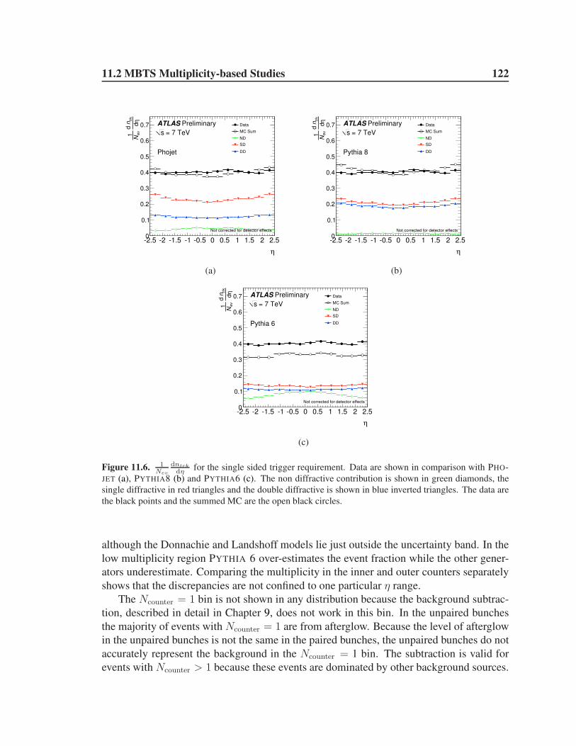
11.2 MBTS Multiplicity-based Studies 122
η
2.5 2 1.5 1 0.5 0 0.5 1 1.5 2 2.5
ηd
trk
nd
ev
N1
0
0.1
0.2
0.3
0.4
0.5
0.6
0.7
Phojet
= 7 TeVs
Not corrected for detector effects
PreliminaryATLAS Data
MC Sum
ND
SD
DD
(a)
η
2.5 2 1.5 1 0.5 0 0.5 1 1.5 2 2.5
ηd
trk
nd
ev
N1
0
0.1
0.2
0.3
0.4
0.5
0.6
0.7
Pythia 8
= 7 TeVs
Not corrected for detector effects
PreliminaryATLAS Data
MC Sum
ND
SD
DD
(b)
η
2.5 2 1.5 1 0.5 0 0.5 1 1.5 2 2.5
ηd
trk
nd
ev
N1
0
0.1
0.2
0.3
0.4
0.5
0.6
0.7
Pythia 6
= 7 TeVs
Not corrected for detector effects
PreliminaryATLAS Data
MC Sum
ND
SD
DD
(c)
Figure 11.6. 1Nev
dntrk
dηfor the single sided trigger requirement. Data are shown in comparison with PHO-
JET (a), PYTHIA8 (b) and PYTHIA6 (c). The non diffractive contribution is shown in green diamonds, the
single diffractive in red triangles and the double diffractive is shown in blue inverted triangles. The data are
the black points and the summed MC are the open black circles.
although the Donnachie and Landshoff models lie just outside the uncertainty band. In the
low multiplicity region PYTHIA 6 over-estimates the event fraction while the other gener-
ators underestimate. Comparing the multiplicity in the inner and outer counters separately
shows that the discrepancies are not confined to one particular η range.
The Ncounter = 1 bin is not shown in any distribution because the background subtrac-
tion, described in detail in Chapter 9, does not work in this bin. In the unpaired bunches
the majority of events with Ncounter = 1 are from afterglow. Because the level of afterglow
in the unpaired bunches is not the same in the paired bunches, the unpaired bunches do not
accurately represent the background in the Ncounter = 1 bin. The subtraction is valid for
events with Ncounter > 1 because these events are dominated by other background sources.
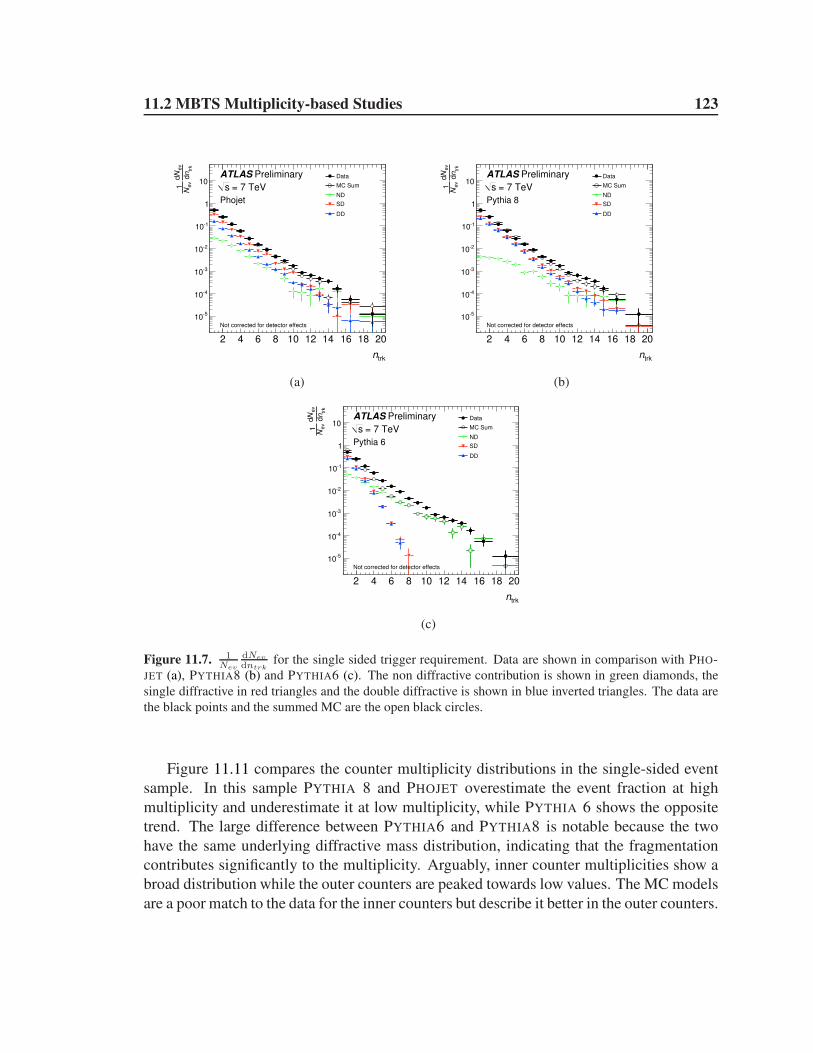
11.2 MBTS Multiplicity-based Studies 123
trkn
2 4 6 8 10 12 14 16 18 20
trk
nd
ev
Nd
ev
N1
510
410
310
210
110
1
10
Phojet
= 7 TeVs
Not corrected for detector effects
PreliminaryATLAS Data
MC Sum
ND
SD
DD
(a)
trkn
2 4 6 8 10 12 14 16 18 20
trk
nd
ev
Nd
ev
N1
510
410
310
210
110
1
10
Pythia 8
= 7 TeVs
Not corrected for detector effects
PreliminaryATLAS Data
MC Sum
ND
SD
DD
(b)
trkn
2 4 6 8 10 12 14 16 18 20
trk
nd
ev
Nd
ev
N1
510
410
310
210
110
1
10
Pythia 6
= 7 TeVs
Not corrected for detector effects
PreliminaryATLAS Data
MC Sum
ND
SD
DD
(c)
Figure 11.7. 1Nev
dNev
dntrkfor the single sided trigger requirement. Data are shown in comparison with PHO-
JET (a), PYTHIA8 (b) and PYTHIA6 (c). The non diffractive contribution is shown in green diamonds, the
single diffractive in red triangles and the double diffractive is shown in blue inverted triangles. The data are
the black points and the summed MC are the open black circles.
Figure 11.11 compares the counter multiplicity distributions in the single-sided event
sample. In this sample PYTHIA 8 and PHOJET overestimate the event fraction at high
multiplicity and underestimate it at low multiplicity, while PYTHIA 6 shows the opposite
trend. The large difference between PYTHIA6 and PYTHIA8 is notable because the two
have the same underlying diffractive mass distribution, indicating that the fragmentation
contributes significantly to the multiplicity. Arguably, inner counter multiplicities show a
broad distribution while the outer counters are peaked towards low values. The MC models
are a poor match to the data for the inner counters but describe it better in the outer counters.

11.3 Summary 124
[GeV]T
p
1 2 3 4 5 6
]2
[G
eV
Tp
d
ηd
trk
n 2
d
Tp
π2
1
ev
N1
610
510
410
310
210
110
1
10
Phojet
= 7 TeVs
Not corrected for detector effects
PreliminaryATLAS Data
MC Sum
ND
SD
DD
(a)
[GeV]T
p
1 2 3 4 5 6
]2
[G
eV
Tp
d
ηd
trk
n 2
d
Tp
π2
1
ev
N1
610
510
410
310
210
110
1
10
Pythia 8
= 7 TeVs
Not corrected for detector effects
PreliminaryATLAS Data
MC Sum
ND
SD
DD
(b)
[GeV]T
p
1 2 3 4 5 6
]2
[G
eV
Tp
d
ηd
trk
n 2
d
Tp
π2
1
ev
N1
610
510
410
310
210
110
1
10
Pythia 6
= 7 TeVs
Not corrected for detector effects
PreliminaryATLAS Data
MC Sum
ND
SD
DD
(c)
Figure 11.8. 1Nev
12πpT
d2ntrk
dηdpTfor the single sided trigger requirement. Data are shown in comparison with
PHOJET (a), PYTHIA8 (b) and PYTHIA6 (c). The non diffractive contribution is shown in green diamonds,
the single diffractive in red triangles and the double diffractive is shown in blue inverted triangles. The data
are the black points and the summed MC are the open black circles.
11.3 Summary
The measurements of the properties of tracks in the diffractive-enhanced sample show
the best agreement with the PHOJET Monte Carlo generator, which accurately reproduces
the charged particle properties and the event level multiplicities. The PYTHIA 8 Monte
Carlo generator reasonably reproduces the η-based distributions and the multiplicities but
does not describe the pT spectrum well. The MBTS multiplicity plots are best reproduced
by PYTHIA 8 with a Donnachie and Landsoff parametrization. However, differences be-
tween PYTHIA 6 and PYTHIA 8 with the Schuler-Sjostrand model show that the agreement
in these variables depends strongly on the fragmentation model. When these results are

11.3 Summary 125
η∆
0 0.5 1 1.5 2 2.5 3 3.5 4 4.5
η∆
dtr
kd
N
ev
N1
0
0.2
0.4
0.6
0.8
1
1.2
Phojet
= 7 TeVs
Not corrected for detector effects
PreliminaryATLAS Data
MC Sum
ND
SD
DD
(a)
η∆
0 0.5 1 1.5 2 2.5 3 3.5 4 4.5
η∆
dtr
kN
d
e
vN
1
0
0.2
0.4
0.6
0.8
1
1.2
Pythia 8
= 7 TeVs
Not corrected for detector effects
PreliminaryATLAS Data
MC Sum
ND
SD
DD
(b)
η∆
0 0.5 1 1.5 2 2.5 3 3.5 4 4.5
η∆
dtr
kN
d
e
vN
1
0
0.2
0.4
0.6
0.8
1
1.2
Pythia 6
= 7 TeVs
Not corrected for detector effects
PreliminaryATLAS Data
MC Sum
ND
SD
DD
(c)
Figure 11.9. 1Nev
dntrk
d∆ηfor the single sided trigger requirement. Data are shown in comparison with PHO-
JET (a), PYTHIA8 (b) and PYTHIA6 (c). The non diffractive contribution is shown in green diamonds, the
single diffractive in red triangles and the double diffractive is shown in blue inverted triangles. The data are
the black points and the summed MC are the open black circles.
taken with the results from minimum bias measurement [70], PYTHIA 8 with a Donnachie
and Landshoff model emerges at the best overall description of inelastic interactions.

11.3 Summary 126
MBTScounterN
5 10 15 20 25 30
MB
TS
counte
rd
N
ev
dN
ev
N1
0
0.02
0.04
0.06
0.08
0.1
0.12
0.14
0.16
0.18
0.2Data 2010
SchulerSjostrand Pythia 6
SchulerSjostrand Pythia 8
Bruni and Ingelman2
’ = 0.25 GeVα = 0.085,∈DL 2
’ = 0.25 GeVα = 0.06, ∈DL 2
’ = 0.25 GeVα = 0.10, ∈DL
Phojet
= 7 TeVs
Inclusive
ATLAS
(a)
MBTScounterN
2 4 6 8 10 12 14 16
MB
TS
co
un
ter
dN
ev
dN
e
vN1
0
0.05
0.1
0.15
0.2
0.25
0.3
0.35Data 2010
SchulerSjostrand Pythia 6
SchulerSjostrand Pythia 8
Bruni and Ingelman2
’ = 0.25 GeVα = 0.085,∈DL 2
’ = 0.25 GeVα = 0.06, ∈DL 2
’ = 0.25 GeVα = 0.10, ∈DL
Phojet
= 7 TeVs
Inclusive
Inner
(b)
MBTScounterN
2 4 6 8 10 12 14 16
MB
TS
co
un
ter
dN
ev
dN
e
vN1
0
0.02
0.04
0.06
0.08
0.1
0.12
0.14
0.16
0.18
0.2
0.22
0.24Data 2010
SchulerSjostrand Pythia 6
SchulerSjostrand Pythia 8
Bruni and Ingelman2
’ = 0.25 GeVα = 0.085,∈DL 2
’ = 0.25 GeVα = 0.06, ∈DL 2
’ = 0.25 GeVα = 0.10, ∈DL
Phojet
= 7 TeVs
Inclusive
Outer
(c)
Figure 11.10. MBTS multiplicity comparing data and MC. (a) shows the inclusive hit distribution, (b) shows
the inclusive inner counter hit multiplicities, and (c) shows the inclusive inner counter hit multiplicities . The
band indicates the systematic uncertainty due to the MBTS response and material.
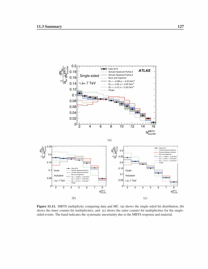
11.3 Summary 127
MBTScounterN
2 4 6 8 10 12 14 16
MB
TS
counte
rd
N
ev
dN
ev
N1
0
0.02
0.04
0.06
0.08
0.1
0.12
0.14
0.16
0.18
0.2Data 2010
SchulerSjostrand Pythia 6
SchulerSjostrand Pythia 8
Bruni and Ingelman2
’ = 0.25 GeVα = 0.085,∈DL 2
’ = 0.25 GeVα = 0.06, ∈DL 2
’ = 0.25 GeVα = 0.10, ∈DL
Phojet
= 7 TeVs
Singlesided
ATLAS
(a)
MBTScounterN
2 3 4 5 6 7 8
MB
TS
co
un
ter
dN
ev
dN
e
vN1
0
0.05
0.1
0.15
0.2
0.25
Data 2010
SchulerSjostrand Pythia 6
SchulerSjostrand Pythia 8
Bruni and Ingelman2
’ = 0.25 GeVα = 0.085,∈DL 2
’ = 0.25 GeVα = 0.06, ∈DL 2
’ = 0.25 GeVα = 0.10, ∈DL
Phojet
= 7 TeVs
Inclusive
Inner
(b)
MBTScounterN
2 3 4 5 6 7 8
MB
TS
co
un
ter
dN
ev
dN
e
vN1
0
0.05
0.1
0.15
0.2
0.25
0.3Data 2010
SchulerSjostrand Pythia 6
SchulerSjostrand Pythia 8
Bruni and Ingelman2
’ = 0.25 GeVα = 0.085,∈DL 2
’ = 0.25 GeVα = 0.06, ∈DL 2
’ = 0.25 GeVα = 0.10, ∈DL
Phojet
= 7 TeVs
Inclusive
Outer
(c)
Figure 11.11. MBTS multiplicity comparing data and MC. (a) shows the single-sided hit distribution, (b)
shows the inner counter hit multiplicities, and (c) shows the outer counter hit multiplicities for the single-
sided events. The band indicates the systematic uncertainty due to the MBTS response and material.

128
CHAPTER 12
Results
This chapter presents the results of the inelastic cross-section measurement using the
inclusive sample defined in Chapter 3. The formula used to calculate the cross-section is
given by Equation 3.12, reproduced here for convenience:
σ(ξ > 5 × 10⁻⁶) =(N −NBG)
ǫtrig × L × CMC. (12.1)
The measurement uses 1.2 million events, N , from run 152221, corresponding to an inte-
grated luminosity, L, of 20.25 µb. Chapter 7 describes the dataset in detail. The trigger
efficiency, ǫtrig , is measured to be 99.98+0.02−0.12%, as described in Chapter 8.2. While the
backgrounds and MBTS performance are described in Chapters 9 and 8, those sections do
not present the corresponding correction factors for the cross-section measurement. In the
following sections the remaining factors necessary to calculate the inelastic cross-section
are determined. In Section 12.1 the number of background events, NBG, is calculated. The
Monte Carlo simulation-based correction factor, CMC, is presented in Section 12.2, which
additionally details the determination of the relative contribution of diffractive events for
each model. Section 12.3 reviews the systematic uncertainties and Section 12.4 presents
the cross-section measurement.
12.1 Background Estimation
This measurement suffers from the primary backgrounds described in Chapter 9: beam-
related backgrounds such as beam-gas, beam-halo and afterglow, and non-beam-related
backgrounds such as noise and cosmic-rays. The measurement corrects for events which
are purely background as inelastic interaction with low activity to migrate into the event
sample because of additional hits supplied by afterglow.
Beam-gas and beam-halo events typically have multiple MBTS counters above thresh-
old, whereas noise and out-of-time afterglow generally produce only one counter above
threshold. These backgrounds are estimated as the sum of events passing the event selec-
tion in the unpaired bunches. In these runs, the same unprescaled trigger is used in the

12.1 Background Estimation 129
Intensity (109 p)
paired unpaired
Beam 1 9.13 9.61
Beam 2 8.77 8.38
Table 12.1. Beam intensities in
terms of protons per bunch for
the paired and unpaired bunches
in run 152221.
paired bunches and in the unpaired bunches. The out-of-time afterglow is overestimated
using this method because the afterglow is correlated with the main collision event in the
preceding paired bunches, as shown in Figure 9.2. Thus, the estimate of background from
unpaired bunches will tend to be an overestimate of the true background contamination.
In order to reduce the effect of afterglow and noise, the event sample is restricted to
events with at least two MBTS hits above threshold. This requirement cuts out the majority
of out-of-time afterglow events which typically have only done counter above threshold. In
principle, it also removes most of the noise-only events, but no events were found to have
a charge less than −0.15 pC. Because the noise is symmetric about 0 pC, it is assumed that
there are no events with noise hits greater than 0.15 pC in the event sample.
The background due to beam gas and beam-halo events is estimated from the unpaired
bunches. Since the afterglow contribution is smaller for BCID=1786 (beam 1) than for
BCID=892 (beam 2), only BCID 1786 is used for the background estimate. However, it
must be corrected for the difference in currents between it and the other bunches. The
correction proceeds as follows
NB1BG = NB1
unp ×IB1p
IB1unp
(12.2)
NB2BG = NB1
unp ×IB1p
IB1unp
×IB2p
IB1p
(12.3)
NBG = NB1unp +NB2
unp (12.4)
= NB1unp ×
IB1p
IB1unp
×(
1 +IB2p
IB1p
)
(12.5)
= 1.86 ×NB1unp (12.6)
Here NB1,2BG is the number of estimated background events in the paired bunches for
Beam 1 or 2, NB1unp is the measured number of events in the unpaired bunches for Beam 1
(BCID 1786), and IB1,2p,unp is the current of the paired or unpaired bunches for Beam 1 or 2.
The beam current values are taken from a database1 and the beam intensities, which are
derived from the currents, are listed in Table 12.1.
Table 12.2 shows the number of observed events in the paired bunches and the esti-
mated background for the single-sided and inclusive event samples with different minimum
MBTS counter requirements.
1The ATLAS conditions database folder /TDAQ/OLC/LHC/LBDATA in COOL.

12.1 Background Estimation 130
Process run 152221
Npaired NBG
Ncounter ≥ 1
single-sided 149518 23737 ± 210
inclusive 1247851 24889 ± 215
Ncounter ≥ 2
single-sided 122490 422 ± 28
inclusive 1220749 1574 ± 54
Table 12.2. Number of events in the paired bunches (Npaired) and estimated background (NBG) for the two
runs we consider for all L1 MBTS 1 triggered events with at least one offline cell above threshold and the
single − sided and the inclusive selection of at least two cells above threshold. The number of background
events is based on the number of events in BCID 1786 and corrected for the difference in currents between
Beam 1 and Beam 2 as defined in 12.2. The uncertainties are statistical only.
The inclusive sample contains 1.2 million events, 10% of which are single-sided. Frac-
tionally, the beam background contributes 0.34% to the single-sided bunches and 0.13% to
the full event sample. The single-sided events make up less than 30% of the background,
indicating that it is mostly from beam-halo events, which produce hits on both sides of the
detector. In contrast, when the event selection requirement is relaxed to only one counter
above threshold, the background is dominantly single-sided and makes up 2% of the in-
clusive sample and 16% of the single-sided sample. This large background is the reason
behind the requirement of at least 2 hits for the cross-section measurement.
Additionally, beam background events can overlap with collision events to increase the
MBTS cell multiplicity. The overlap is a problem for the single-sided sample because it
could cause a single-sided event to appear as a double-sided event. However, the luminosity
of this run was low enough that there were only 0.007 events per crossing. There are
roughly 2% as many events with Ncounter ≥ 1 in the unpaired bunches as in the paired
bunches, leading to a beam background event every 0.0001 crossings. Therefore, an overlap
occurs in 0.01% of the event sample, which is negligible.
Lastly, the contribution from in-time afterglow, which is not modeled in the Geant4
simulation, is estimated. Afterglow hits arising from collisions with less than 2 prompt
MBTS hits could cause the events migrate into the event sample. As described in Chap-
ter 9 the asymmetry of the time of the MBTS hits is used as an upper limit on the in-time
afterglow contribution.
Binomial statistics are used to find the fraction of events with two real hits, freal, as a
function of the number of observed counters over threshold:
freal(N) =
N∑
n=2
(
N
n
)
h.p.(N)n(1 − h.p.(N))N−n (12.7)
freal(2) = h.p.(2)2 (12.8)
freal(3) = h.p.(3)3 + 3h.p.(3)2(1 − h.p.(3)) (12.9)
where N = Ncounter, the number of counters over threshold.

12.2 Acceptance 131
The hit purity of the Ncounter = 2 and Ncounter = 3 events was found to be 0.83.
Therefore 67% of events with Ncounter = 2 have two real hits and 92% of the events with
Ncounter = 3 have at least two real hits. Ncounter = 2 and Ncounter = 3 each make up
approximately 1% of the event sample and therefore, 0.4% of events in the selected events
sample have less than two real hits. In the single-sided sample, the Ncounter = 2 and
Ncounter = 3 events each make up approximately 10% of the event sample. The afterglow
is at most 3.6% of this sample.
An uncertainty of 100% is assumed on both the in-time afterglow and other beam-
related background determinations. The resulting uncertainties are added in quadrature.
This conservative estimate is due to the fact that the afterglow contribution is not well-
understood but it is clear that it can only be overestimated using these methods. The un-
certainties from other sources, such as the beam-current ratios, are small compared to the
afterglow uncertainty.
12.2 Acceptance
This section discusses the acceptance of the event selection as determined with Monte
Carlo models. First, the MBTS detector acceptance is discussed for the diffractive and non-
diffractive sub-processes in Section 12.2.1. Then, the data are used to constrain the relative
diffractive cross-sections in Section 12.2.2. A determination of ǫsel and fξ<5×10⁻⁶ for the
measurement range follows in Section 12.2.3. Finally, the extrapolation to ξ > m2P/s is
discussed in Section 12.2.4.
12.2.1 MBTS Acceptance
The MBTS acceptance for the inclusive and the single-sided selections are given in
Table 12.3. The inclusive values are very high for the non-diffractive component for all
generators, while it is as low as 43% for some of the diffractive contributions. The single-
sided numbers show that the non-diffractive component is significantly suppressed for this
selection: less than 1% of the ND events are selected. For the diffractive components ǫselvaries between 27 and 41%. The effect of variations in the Monte Carlo tuning was investi-
gated using several different PYTHIA 6 tunes2. The differences between the tunings in the
acceptance were smaller than the differences between the MC models, and therefore the
tuning was not considered in further studies. This large variation in acceptance motivates
the restriction of the measurement to a well-defined ξ-range. It also motivates constraining
the relative diffractive contribution to the cross-section.
Figure 12.1 shows the efficiency of the MBTS selection (ǫSel) as a function of ξ and
ηmin3. The efficiency agrees between the different generators to within 5% as a function
2Perugia0 and DW were used for all three subprocesses, and there were serveral other variations of inital
and final state parameters for non-diffractive events only.3ηmin is defined in Chapter 3
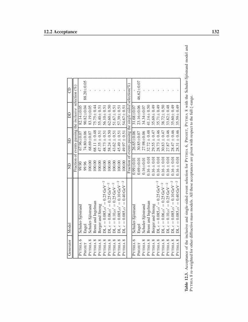
12.2 Acceptance 132
Gen
erat
or
Mo
del
ND
SD
DD
CD
Fra
ctio
no
fev
ents
pas
sin
gth
ein
clu
sive
sele
ctio
n(%
)
PY
TH
IA6
Sch
ule
r-S
jost
ran
d9
9.9
06
7.9
6±
0.0
78
2.1
4±
0.0
5-
PH
OJE
TE
ng
el9
9.9
67
4.8
0±
0.0
69
0.8
2±
0.0
48
8.2
0±
0.0
5
PY
TH
IA8
Sch
ule
r-S
jost
ran
d1
00
.00
68
.69±
0.0
78
3.1
9±
0.0
5-
PY
TH
IA8
Bru
ni
and
Ing
elm
an1
00
.00
68
.11±
0.4
87
5.7
5±
0.4
4-
PY
TH
IA8
Ber
ger
and
Str
eng
10
0.0
04
7.3
5±
0.5
15
5.4
0±
0.5
1-
PY
TH
IA8
DL
ǫ=
0.0
85
,α′=
0.2
5G
eV−
21
00
.00
48
.73±
0.5
15
6.1
0±
0.5
1-
PY
TH
IA8
DL
ǫ=
0.0
6,α
′=
0.2
5G
eV−
21
00
.00
58
.24±
0.5
06
2.6
0±
0.5
0-
PY
TH
IA8
DL
ǫ=
0.1
0,α
′=
0.2
5G
eV−
21
00
.00
43
.62±
0.5
15
1.6
7±
0.5
1-
PY
TH
IA8
DL
ǫ=
0.0
85
,α′=
0.1
0G
eV−
21
00
.00
45
.49±
0.5
15
7.3
9±
0.5
1-
PY
TH
IA8
DL
ǫ=
0.0
85
,α′=
0.4
0G
eV−
21
00
.00
49
.97±
0.5
15
4.6
7±
0.5
1-
Fra
ctio
no
fev
ents
pas
sin
gth
esi
ng
le-s
ided
sele
ctio
n(%
)
PY
TH
IA6
Sch
ule
r-S
jost
ran
d0
.99±
0.0
12
6.6
5±
0.0
63
1.6
8±
0.0
7-
PH
OJE
TE
ng
el0
.69±
0.0
13
0.8
5±
0.0
72
3.1
6±
0.0
64
6.6
2±
0.0
7
PY
TH
IA8
Sch
ule
r-S
jost
ran
d0
.16±
0.0
12
7.9
8±
0.0
63
4.3
4±
0.0
7-
PY
TH
IA8
Bru
ni
and
Ing
elm
an0
.16±
0.0
13
2.7
2±
0.4
84
1.1
4±
0.5
0-
PY
TH
IA8
Ber
ger
and
Str
eng
0.1
6±
0.0
12
9.5
5±
0.4
73
5.6
9±
0.4
9-
PY
TH
IA8
DL
ǫ=
0.0
85
,α′=
0.2
5G
eV−
20
.16±
0.0
12
8.7
3±
0.4
63
5.7
1±
0.4
9-
PY
TH
IA8
DL
ǫ=
0.0
6,α
′=
0.2
5G
eV−
20
.16±
0.0
13
0.8
3±
0.4
73
8.7
2±
0.5
0-
PY
TH
IA8
DL
ǫ=
0.1
0,α
′=
0.2
5G
eV−
20
.16±
0.0
12
7.8
7±
0.4
63
3.8
2±
0.4
8-
PY
TH
IA8
DL
ǫ=
0.0
85
,α′=
0.1
0G
eV−
20
.16±
0.0
12
8.4
7±
0.4
63
5.6
0±
0.4
9-
PY
TH
IA8
DL
ǫ=
0.0
85
,α′=
0.4
0G
eV−
20
.16±
0.0
12
8.3
1±
0.4
63
5.5
9±
0.4
9-
Ta
ble
12
.3.
Acc
epta
nce
of
the
incl
usi
ve
and
sin
gle
-sid
edev
ent
sele
ctio
nfo
rP
YT
HIA
6,
PH
OJE
T,
PY
TH
IA8
wit
hth
eS
chu
ler-
Sjo
stra
nd
mo
del
and
PY
TH
IA8
re-w
eig
hte
dfo
ro
ther
dif
frac
tive
mas
sm
od
els.
All
thes
eac
cep
tan
ces
are
giv
enw
ith
resp
ect
toth
efu
llξ-
ran
ge.

12.2 Acceptance 133
)ξ(10
log
8 7 6 5 4 3 2 1 0
Se
l∈
0
0.2
0.4
0.6
0.8
1SD
Pythia 8
Phojet
Pythia 6
(a)
)ξ(10
log
8 7 6 5 4 3 2 1 0
Se
l∈
0
0.2
0.4
0.6
0.8
1
Phojet DD
Phojet SD
(b)
)ξ(10
log
7 6 5 4 3 2 1 0
Sel
∈
0
0.2
0.4
0.6
0.8
1SD
Pythia 8
Phojet
Pythia 6
(c)
)ξ(10
log
7 6 5 4 3 2 1 0
Sel
∈
0
0.2
0.4
0.6
0.8
1DD
Pythia 8
Phojet
Pythia 6
(d)
Figure 12.1. Efficiency of the inclusive MBTS selection as a function of log10(ξ) for single-diffractive (a)
comparing PYTHIA 6, PYTHIA 8, and PHOJET. A comparison of the efficiency between single- and double-
dissociation (b) events for PHOJET. (c) and (d) show the same efficiency as a function of ηmin. In the case
of double-dissociation the higher mass system is plotted.
of ξ and ηMin for the SD processes, and to within 8% for the DD processes. The SD and
DD efficiencies agree to within 8% as a function of ξ and 10% as a function of ηMin. At
ξ = 5×10⁻⁶ the MBTS selection is 50% efficient. The large width of the efficiency turn on
in ηmin is due to the requirement of at least 2 MBTS hits over threshold, which effectively
requires a second particle to also be within the acceptance.
Figure 12.2 shows the efficiency of the single-sided selection for single- and double-
dissociation events as a function of the maximum diffractive mass in the event. While all
of the generators have the same turn-on and turn-off in efficiency with diffractive mass,
they achieve different plateau values. The higher multiplicity generators, PHOJET and
PYTHIA 8 have similar behavior for the single-dissociation events, but differ for the double-
dissociation events. The difference is likely due to the correlations between the two disso-
ciation systems in these events.

12.2 Acceptance 134
)max
ξ(10
log
8 7 6 5 4 3 2 1 0
SS
∈
0
0.2
0.4
0.6
0.8
1
SDPythia 8
Phojet
Pythia 6
(a)
)max
ξ(10
log
8 7 6 5 4 3 2 1 0
SS
∈
0
0.2
0.4
0.6
0.8
1
DDPythia 8
Phojet
Pythia 6
(b)
Figure 12.2. Efficiency of the single-sided MBTS selection as a function of log10(ξ) for single-diffractive (a)
and double-diffractive (b) events comparing PYTHIA 6 , PYTHIA 8 and PHOJET . In the case of double-
dissociation the higher mass system is plotted.
12.2.2 Fractional Contribution of Diffractive Processes
As seen in Table 12.3, the single-sided selection strongly suppresses non-diffractive
events. Consequently, the quantity fD can be determined experimentally from RSS, the
fraction of events in the inclusive sample that have hits on only one side of the MBTS
detector. The dependence of RSS on fD is outlined in Equation 3.10.
Table 12.4 lists the values obtained by the MC generators for RSS.
RSS = [10.02 ± 0.03(stat.)+0.07−0.36(sys.)]%
is measured for the inclusive sample in data. The systematic uncertainties on RSS include
the MBTS response, backgrounds, and the material effects, which are described in Chap-
ters 8, 9 and 8.4, respectively.
Assuming the acceptance values from Table 12.3, RSS is predicted as a function of
the relative diffractive contributions (fD and fSD). For the models without full simulation,
PYTHIA 8 events are re-weighted to match the ξ distribution described by each model. In
Fig. 12.3 fD is varied, keeping fSD fixed at the value predicted by the relevant generator
(see Table 2.1). It is seen that the preferred value for fD varies between 25% and 30%
depending on the model. Because the relative DD to SD contributions are also not well
known, σDD/σSD, is also varied. Figure 12.4 shows the predictions assuming σDD/σSD = 1and σDD/σSD = 0 as two extreme choices. 4.
The maximum and minimum allowed values of fD are determined from the measured
value of RSS by taking the intersection of the MC predictions with the systematic error
band of the data. The values are determined for each of the models separately and for the
4σDD/σSD = 1 is an extreme choice because for reasonable models of diffractive processes, the DD
component does not exceed the SD component until s >> 100 TeV [60].

12.2 Acceptance 135
Generator Model RSS (%)
PYTHIA 6 Schuler-Sjostrand 10.83 ± 0.01
PHOJET Engel 6.85 ± 0.01
PYTHIA 8 Schuler-Sjostrand 10.83 ± 0.01
PYTHIA 8 Bruni and Ingelman 12.94 ± 0.1
PYTHIA 8 Berger and Streng 12.39 ± 0.1
PYTHIA 8 DL ǫ = 0.085,α′ = 0.25 GeV−2 12.16 ± 0.1
PYTHIA 8 DL ǫ = 0.02,α′ = 0.25 GeV−2 12.56 ± 0.1
PYTHIA 8 DL ǫ = 0.15,α′ = 0.25 GeV−2 9.98 ± 0.1
PYTHIA 8 DL ǫ = 0.085,α′ = 0.10 GeV−2 12.15 ± 0.1
PYTHIA 8 DL ǫ = 0.085,α′ = 0.40 GeV−2 12.04 ± 0.1
Table 12.4. Predicted values for RSS at√
s = 7 TeV for PYTHIA 6, PHOJET, PYTHIA 8 with the Schuler-
Sjostrand model and PYTHIA 8 re-weighted for other diffractive mass models.
variations of σDD/σSD. The results are listed in Table 12.5. The fitted fD value is average
of fminD and fmax
D for the default σDD/σSD and the error is the spread in allowed fD values
for σDD
σSD= 1 and σDD
σSD= 0. The central values range from 25% to 30% and the error is
typically between 1% and 3%. It is interesting to note that although the exclusive particle
properties of the PYTHIA 8 and PYTHIA 6 are very different, they prefer a very similar
value of fD. This similarity suggests that the RSS measurement is primarily sensitive to the
differential diffractive mass distribution rather than the diffractive event modeling.
12.2.3 ǫsel and fξ<5×10⁻⁶
The kinematic range of the measurement is restricted by defining the acceptance with
respect to a limited diffractive mass range, as described in Section 3.
Table 12.6 lists the fraction of events with ξ > 5 × 10⁻⁶ that pass the event selection
(ǫsel) as well as fξ<5×10⁻⁶ , the fraction of events in the inclusive event sample that have
ξ < 5 × 10⁻⁶. ǫsel is greater than 90% for all processes, generators and diffractive mass
spectra. When the ND, SD, and DD components are combined with the value of fD in
Table 12.5 the inelastic efficiencies are between 98.5 and 99.5 %. fξ<5×10⁻⁶ varies more
significantly. It is as low as 1.2% and as high as 8.3% for the diffractive processes. It is
consistent with 0 for the ND process. The large variations in fξ<5×10⁻⁶ for the diffractive
processes are attributed to differences in the diffractive mass spectra at low ξ. The total
inelastic fξ<5×10⁻⁶ varies between 0.3 and 1%.
12.2.4 Extrapolating to ξ > m2p/s
In order to extrapolate from σ(ξ > 5× 10⁻⁶) to σinel, the fraction of the inelastic cross-
section within the kinematic range of the measurement (ξ > 5 × 10⁻⁶) is determined for
each model. Table 12.7 gives the fraction of events that fulfill the ξ > 5 × 10⁻⁶ cut for
the individual processes, i.e. σ(ξ > 5 × 10⁻⁶)/σinel. This fraction is nearly 100% for all

12.2 Acceptance 136
Gen
erat
or
Mo
del
def
ault
σD
D
σSD
σD
D
σSD
=0
σD
D
σSD
=1
fitt
edf D
fm
inD
fm
ax
Df
min
Df
max
Df
min
Df
max
D
PY
TH
IA6
Sch
ule
r-S
jost
ran
d2
8.6
29
.93
1.0
31
.42
8.3
29
.629.3
+2.1
−0.9
PH
OJE
TE
ng
el2
8.7
29
.92
6.7
27
.93
0.7
32
.029.3
+2.7
−2.6
PY
TH
IA8
Sch
ule
r-S
jost
ran
d2
9.0
30
.23
1.2
32
.42
8.6
29
.829.6
+2.8
−1.0
PY
TH
IA8
Bru
ni
and
Ing
elm
an2
4.5
25
.52
6.7
27
.82
4.1
25
.125.0
+2.8
−0.9
PY
TH
IA8
Ber
ger
and
Str
eng
26
.02
6.9
27
.62
8.6
25
.62
6.6
26.4
+2.2
−0.8
PY
TH
IA8
DL
ǫ=
0.0
85
,α′=
0.2
5G
eV−
22
6.4
27
.42
8.4
29
.42
5.9
26
.92
6.9
+2.5
−1.0
PY
TH
IA8
DL
ǫ=
0.0
6,α
′=
0.2
5G
eV−
22
5.3
26
.22
7.5
28
.52
4.8
25
.72
5.7
+2.8
−0.9
PY
TH
IA8
DL
ǫ=
0.1
0,α
′=
0.2
5G
eV−
22
7.1
28
.02
8.8
29
.72
6.7
27
.62
7.5
+2.2
−0.8
PY
TH
IA8
DL
ǫ=
0.0
85
,α′=
0.1
0G
eV−
22
6.4
27
.42
8.3
29
.42
6.0
27
.02
6.9
+2.5
−0.9
PY
TH
IA8
DL
ǫ=
0.0
85
,α′=
0.4
0G
eV−
22
6.6
27
.62
8.8
29
.92
6.1
27
.12
7.1
+2.8
−1.0
Ta
ble
12
.5.
Min
imu
man
dm
axim
um
f Dval
ues
allo
wed
by
the
RSS
mea
sure
men
tfo
rth
eM
Cm
od
els
for
dif
fere
nt
assu
mp
tio
ns
on
f SD
asd
eriv
edfr
om
the
incl
usi
ve
RSS
mea
sure
men
t.T
he
last
colu
mn
show
sth
efi
tted
val
ue
off D
for
each
gen
erat
or
and
the
un
cert
ain
tyd
eriv
edfr
om
the
var
iati
on
so
ff S
D.
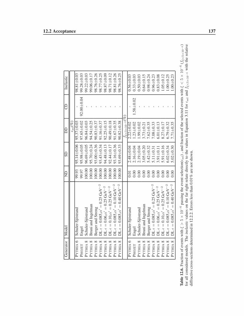
12.2 Acceptance 137
Gen
erat
or
Mo
del
ND
SD
DD
CD
Inel
asti
c
ǫ sel(
%)
PY
TH
IA6
Sch
ule
r-S
jost
ran
d9
9.9
39
5.1
4±
0.0
69
5.3
7±
0.0
3-
98
.81±
0.0
3
PH
OJE
TE
ng
el9
9.9
79
5.9
8±
0.0
59
7.6
5±
0.0
29
2.0
0±
0.0
49
9.2
8±
0.0
3
PY
TH
IA8
Sch
ule
r-S
jost
ran
d1
00
.00
96
.69±
0.0
59
6.8
4±
0.0
3-
99
.22±
0.0
3
PY
TH
IA8
Bru
ni
and
Ing
elm
an1
00
.00
95
.70±
0.2
49
4.5
4±
0.2
5-
99
.06±
0.1
7
PY
TH
IA8
Ber
ger
and
Str
eng
10
0.0
09
3.0
0±
0.3
69
0.8
3±
0.3
7-
98
.76±
0.2
6
PY
TH
IA8
DL
ǫ=
0.0
85
,α′=
0.2
5G
eV−
21
00
.00
93
.43±
0.3
49
1.1
6±
0.3
7-
98
.77±
0.2
5
PY
TH
IA8
DL
ǫ=
0.0
6,α
′=
0.2
5G
eV−
21
00
.00
94
.48±
0.1
39
2.2
5±
0.1
5-
98
.87±
0.0
9
PY
TH
IA8
DL
ǫ=
0.1
0,α
′=
0.2
5G
eV−
21
00
.00
92
.44±
0.1
79
0.4
9±
0.1
8-
98
.71±
0.1
2
PY
TH
IA8
DL
ǫ=
0.0
85
,α′=
0.1
0G
eV−
21
00
.00
93
.16±
0.3
69
1.6
7±
0.3
5-
98
.81±
0.2
6
PY
TH
IA8
DL
ǫ=
0.0
85
,α′=
0.4
0G
eV−
21
00
.00
93
.69±
0.3
39
0.8
2±
0.3
8-
98
.76±
0.2
5
f ξ<
5×
10−
6(%
)
PY
TH
IA6
Sch
ule
r-S
jost
ran
d0
.01
2.4
8±
0.0
42
.22±
0.0
2-
0.5
6±
0.0
3
PH
OJE
TE
ng
el0
.00
2.1
6±
0.0
41
.23±
0.0
21
.58±
0.0
20
.33±
0.0
3
PY
TH
IA8
Sch
ule
r-S
jost
ran
d0
.00
2.1
9±
0.0
41
.99±
0.0
2-
0.5
0±
0.0
3
PY
TH
IA8
Bru
ni
and
Ing
elm
an0
.00
3.0
5±
0.2
03
.73±
0.2
1-
0.6
4±
0.1
5
PY
TH
IA8
Ber
ger
and
Str
eng
0.0
05
.42±
0.3
27
.62±
0.3
5-
0.9
8±
0.2
4
PY
TH
IA8
DL
ǫ=
0.0
85
,α′=
0.2
5G
eV−
20
.00
5.1
1±
0.3
17
.08±
0.3
3-
0.9
6±
0.2
3
PY
TH
IA8
DL
ǫ=
0.0
6,α
′=
0.2
5G
eV−
20
.00
3.9
1±
0.1
16
.01±
0.1
3-
0.8
3±
0.0
8
PY
TH
IA8
DL
ǫ=
0.1
0,α
′=
0.2
5G
eV−
20
.00
5.9
1±
0.1
68
.27±
0.1
7-
1.0
5±
0.1
2
PY
TH
IA8
DL
ǫ=
0.0
85
,α′=
0.1
0G
eV−
20
.00
6.0
2±
0.3
46
.79±
0.3
2-
1.0
0±
0.2
5
PY
TH
IA8
DL
ǫ=
0.0
85
,α′=
0.4
0G
eV−
20
.00
5.0
2±
0.3
07
.71±
0.3
5-
1.0
0±
0.2
3
Ta
ble
12
.6.
Fra
ctio
no
fev
ents
wit
hξ
>5×
10−
6p
assi
ng
the
even
tse
lect
ion
(ǫse
l),
and
frac
tio
no
fth
ese
lect
edev
ents
wit
hξ
<5×
10−
6(f
ξ<
5×
10−
6)
for
all
con
sid
ered
mo
del
s.T
he
inel
ast
icval
ues
on
the
far
rig
ht
rela
ted
irec
tly
toth
eval
ues
inE
qu
atio
n3
.11
forǫ s
el
and
f ξ<
5×
10−
6w
ith
the
rela
tive
dif
frac
tive
cro
ss-s
ecti
on
sd
eter
min
edin
12
.2.2
.E
rro
rsle
ssth
an0
.01
%ar
en
ot
show
n.

12.3 Systematic Uncertainties 138
Df
0.1 0.15 0.2 0.25 0.3 0.35 0.4
ss
R
0.04
0.06
0.08
0.1
0.12
0.14
0.16
0.18 Data 2010
strand Pythia 6oSchulerSj
strand Pythia 8oSchulerSj
Bruni and Ingelman Pythia 8
= 0.085 Pythia 8εDL
= 0.06 Pythia 8εDL
= 0.10 Pythia 8εDL
Phojet
= 7 TeVs
ATLAS
Figure 12.3. RSS versus fD. The data are shown as the line with systematic uncertainties (grey band). Also
shown are the predictions as a function of fD for a variety of models. For each model th point indicates the
predicted value of RSS for the default value of fD. In this case the default value for fSD is assumed for each
sample, i.e. 59.6% for PYTHIA and additional models and 68.6% for PHOJET. For all models but PHOJET
the σCD is taken to be 0.
models of the ND processes, whereas it varies between 44% and 76% for the SD events
and between 53% and 92% for the DD events depending on the assumed ξ-dependence of
the diffractive cross section. Additionally, there are predictions from M. Ryskin based on
the work in [51] which predicts σ(ξ > 5 × 10⁻⁶)/σinel = 77 − 82%.
To perform the extrapolation of the cross-section measurement from the restricted ξ-
range to the full range, the model by Donnachie and Landshoff with ǫ = 0.085 and
α′ =0.25 GeV−2 is used because it gives the best description of the MBTS hit multiplicity
for the single-sided sample (see Fig. 11.11). It predicts 87.2% acceptance for the ξ cut.
The lowest acceptance value is obtained with the Ryskin model. The highest fraction is
given by the Engel model, which predicts 95% of the cross-section to have ξ > 5 × 10⁻⁶.
The full spread of the acceptance value is taken as a systematic uncertainty, leading to an
extrapolation factor of 1.145 ± 0.115.
12.3 Systematic Uncertainties
The systematic errors on the total cross section measurement are summarized in Ta-
ble 12.8. The following sources contribute to the total uncertainty:

12.3 Systematic Uncertainties 139
Gen
erat
or
Mo
del
ND
SD
DD
CD
Inel
asti
c
Fra
ctio
no
fev
ents
wit
hξ
>5×
10−
6(%
)
PY
TH
IA6
Sch
ule
r-S
jost
ran
d9
9.9
66
9.7
2±
0.1
08
4.2
2±
0.0
5-
92
.82±
0.0
4
PH
OJE
TE
ng
el9
9.9
87
6.1
0±
0.1
09
1.8
6±
0.0
49
4.3
5±
0.0
39
6.0
1±
0.0
3
PY
TH
IA8
Sch
ule
r-S
jost
ran
d1
00
.00
69
.58±
0.1
08
4.1
9±
0.0
5-
92
.74±
0.0
4
PY
TH
IA8
Bru
ni
and
Ing
elm
an1
00
.00
69
.02±
0.4
57
7.2
9±
0.4
1-
93
.06±
0.3
0
PY
TH
IA8
Ber
ger
and
Str
eng
10
0.0
04
8.1
7±
0.4
95
6.5
4±
0.4
8-
87
.21±
0.3
3
PY
TH
IA8
DL
ǫ=
0.0
85
,α′=
0.2
5G
eV−
21
00
.00
49
.51±
0.4
95
7.3
7±
0.4
8-
87
.27±
0.3
3
PY
TH
IA8
DL
ǫ=
0.0
6,α
′=
0.2
5G
eV−
21
00
.00
59
.25±
0.2
16
3.9
6±
0.2
1-
90
.02±
0.1
2
PY
TH
IA8
DL
ǫ=
0.1
0,α
′=
0.2
5G
eV−
21
00
.00
44
.41±
0.2
25
2.5
7±
0.2
2-
85
.62±
0.1
3
PY
TH
IA8
DL
ǫ=
0.0
85
,α′=
0.1
0G
eV−
21
00
.00
45
.91±
0.4
95
8.5
4±
0.4
8-
86
.82±
0.3
3
PY
TH
IA8
DL
ǫ=
0.0
85
,α′=
0.4
0G
eV−
21
00
.00
50
.67±
0.4
95
5.7
4±
0.4
8-
87
.19±
0.3
3
Ta
ble
12
.7.
Fra
ctio
no
fev
ents
wit
hξ
>5×
10−
6fo
ral
lco
nsi
der
edm
od
els.
Th
em
ost
rig
ht-
han
dco
lum
nca
nb
eu
nd
erst
oo
din
term
so
fE
qu
atio
ns
3.1
and
3.1
1as
σ(ξ
>5×
10−
6)/
σin
el.
Th
eval
ues
for
the
rela
tive
dif
frac
tive
cro
ss-s
ecti
on
det
erm
ined
in1
2.2
.2.
Wh
enth
eer
ror
isn
ot
show
nit
isle
ssth
an
0.0
1.

12.3 Systematic Uncertainties 140
Df
0.1 0.15 0.2 0.25 0.3 0.35 0.4
ss
R
0.04
0.06
0.08
0.1
0.12
0.14
0.16
0.18 Data 2010
strand Pythia 6oSchulerSj
strand Pythia 8oSchulerSj
Bruni and Ingelman Pythia 8
= 0.085 Pythia 8εDL
= 0.06 Pythia 8εDL
= 0.10 Pythia 8εDL
Phojet
= 7 TeVs
= 0SD
σDD
σ
(a)
Df
0.1 0.15 0.2 0.25 0.3 0.35 0.4
ss
R
0.04
0.06
0.08
0.1
0.12
0.14
0.16
0.18 Data 2010
strand Pythia 6oSchulerSj
strand Pythia 8oSchulerSj
Bruni and Ingelman Pythia 8
= 0.085 Pythia 8εDL
= 0.06 Pythia 8εDL
= 0.10 Pythia 8εDL
Phojet
= 7 TeVs
= 1SD
σDD
σ
(b)
Figure 12.4. RSS versus fD with σDD
σSD= 1 (a) and σDD
σSD= 0 (b). The data are shown as the line with
systematic uncertainties (grey band). Also shown are the predictions for a variety of models as function of an
assumed value of fD.
• MBTS trigger efficiency: The efficiency of the trigger requirement with respect to
the offline requirement of two MBTS hits is studied in data as described in Chap-
ter 8.2. The trigger efficiency is measured with randomly triggered events to be
99.98+0.02−0.12%. In order to set a systematic uncertainty, a trigger requiring at least one
hit in the LUCID detector (5.6 < |η| < 6.0) is used to independently determine the
efficiency. This method yields an efficiency of 99.91%. The difference between the
LUCID based and random trigger based methods is taken as the uncertainty. Both
methods agree within the statistical uncertainties and 0.07% is taken as the uncer-
tainty.
• MBTS response: Chapter 8 showed that the data and MC simulation disagree in the
shape of the signal charge distribution, leading to a lower average counter efficiency
in the data. This effect is emulated in the MC by increasing the threshold to 0.28 pC
(0.26 pC) on the A- (C-) side outer counters and 0.32 pC (0.38 pC) on the A- (C-
) side inner counters. The systematic uncertainty associated with tuning the MBTS
efficiency in the simulation is obtained by varying the MC thresholds until they match
the efficiency of the counter in data which is furthest from the mean counter efficiency
on each side and ring. The resulting thresholds are 0.50 (0.60) pC for the A- (C-) side
inner counters and 0.18 (0.38) pC for the A- (C-) side outer counters. Changing the
MC thresholds to these values results in a 0.09% variation on CMC for PYTHIA6 and
in smaller variations for the other models. Thus 0.1% is taken as the uncertainty due
to the MBTS response.
• Beam background determination: As described in Chapter 9 and Section 12.1,
the background contribution is estimated from the unpaired bunches and from the

12.4 The Cross-section Measurement 141
asymmetry of the MBTS counter time measurement. Conservatively, 100% error
is assumed on the beam background, leading to a 0.42% uncertainty on the cross
section measurement.
• Luminosity: The uncertainty on the luminosity was described in detail in Chapter 10.
The 3.4% uncertainty is dominated by the uncertainty on the measurement of the
beam currents.
• Acceptance: The acceptance correction uncertainty is divided into several parts:
– Relative diffractive cross-section: The value of fD preferred by the data and
its uncertainty is determined for each MC model as described in Section 12.2.2.
The difference in CMC obtained using the spread of the allowed fD values (Ta-
ble 12.5) is set as the systematic uncertainty. This variation leads to a symmetric
0.26% uncertainty on CMC determined with the Donnachie and Landshoff ǫ =0.085,α′ = 0.25 GeV−2 parametrization.
– MC Multiplicity: The dependence of the correction factor on the multiplicity
of the diffractive system was determined by the taking the difference between
CMC determined with PYTHIA 8 and PYTHIA 6. These two models have the
same cross-section model but quite different particle multiplicity distributions
for diffractive events. The difference leads to a 0.36% uncertainty on CMC.
– ξ-dependence : The dependence on the input diffractive mass distribution is
determined by comparing the value of CMC for all models. The maximum
difference between the Donnachie and Landshoff ǫ = 0.085, α′ = 0.25 GeV−2
model with all other models is taken as the uncertainty. The largest difference
comes from the PHOJET prediction and results in a 0.36% uncertainty on CMC.
• Material: An excess in material with respect to the model used for simulation in-
creases the MBTS multiplicity due to the increased rate of conversions as well as
increased scattering. The effect of material is evaluated by taking twice the differ-
ence in CMC of the PYTHIA 6 MC simulated with the nominal and extra material
geometries as described in Section 8.4. This contributes 0.20% to the uncertainty on
the cross-section measurement.
The CD process is only included in PHOJET. Including or not including this process in
PHOJET makes a 0.01% difference to CMC which is negligible compared to the systematic
uncertainties listed above. Therefore, there is no additional uncertainty due to the CD
contribution.
12.4 The Cross-section Measurement
The final result depends upon CMC: the combination of ǫSel and fξ<5×10⁻⁶ . Using the
calculated ǫSel and fξ<5×10⁻⁶ values in Table 12.6 and the relative diffractive contribution,
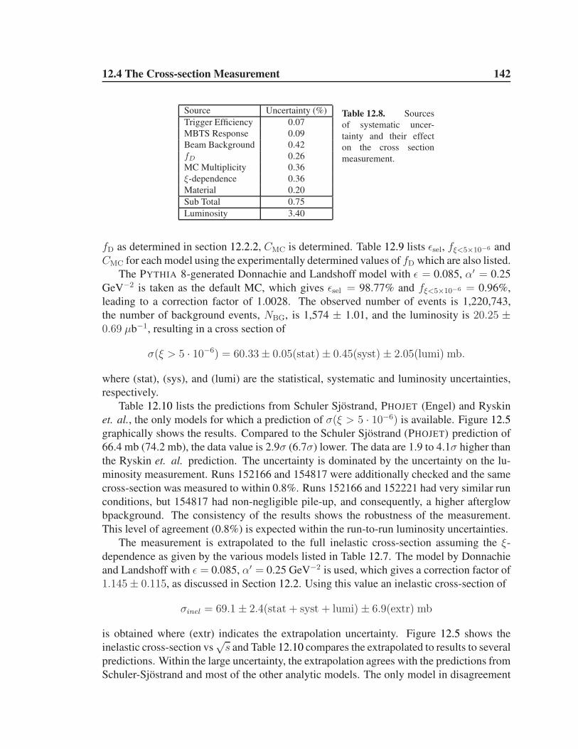
12.4 The Cross-section Measurement 142
Source Uncertainty (%)
Trigger Efficiency 0.07
MBTS Response 0.09
Beam Background 0.42
fD 0.26
MC Multiplicity 0.36
ξ-dependence 0.36
Material 0.20
Sub Total 0.75
Luminosity 3.40
Table 12.8. Sources
of systematic uncer-
tainty and their effect
on the cross section
measurement.
fD as determined in section 12.2.2, CMC is determined. Table 12.9 lists ǫsel, fξ<5×10⁻⁶ and
CMC for each model using the experimentally determined values of fD which are also listed.
The PYTHIA 8-generated Donnachie and Landshoff model with ǫ = 0.085, α′ = 0.25
GeV−2 is taken as the default MC, which gives ǫsel = 98.77% and fξ<5×10−6 = 0.96%,
leading to a correction factor of 1.0028. The observed number of events is 1,220,743,
the number of background events, NBG, is 1,574 ± 1.01, and the luminosity is 20.25 ±0.69 µb−1, resulting in a cross section of
σ(ξ > 5 · 10−6) = 60.33 ± 0.05(stat) ± 0.45(syst) ± 2.05(lumi) mb.
where (stat), (sys), and (lumi) are the statistical, systematic and luminosity uncertainties,
respectively.
Table 12.10 lists the predictions from Schuler Sjostrand, PHOJET (Engel) and Ryskin
et. al., the only models for which a prediction of σ(ξ > 5 · 10−6) is available. Figure 12.5
graphically shows the results. Compared to the Schuler Sjostrand (PHOJET) prediction of
66.4 mb (74.2 mb), the data value is 2.9σ (6.7σ) lower. The data are 1.9 to 4.1σ higher than
the Ryskin et. al. prediction. The uncertainty is dominated by the uncertainty on the lu-
minosity measurement. Runs 152166 and 154817 were additionally checked and the same
cross-section was measured to within 0.8%. Runs 152166 and 152221 had very similar run
conditions, but 154817 had non-negligible pile-up, and consequently, a higher afterglow
bpackground. The consistency of the results shows the robustness of the measurement.
This level of agreement (0.8%) is expected within the run-to-run luminosity uncertainties.
The measurement is extrapolated to the full inelastic cross-section assuming the ξ-
dependence as given by the various models listed in Table 12.7. The model by Donnachie
and Landshoff with ǫ = 0.085, α′ = 0.25 GeV−2 is used, which gives a correction factor of
1.145 ± 0.115, as discussed in Section 12.2. Using this value an inelastic cross-section of
σinel = 69.1 ± 2.4(stat + syst + lumi) ± 6.9(extr) mb
is obtained where (extr) indicates the extrapolation uncertainty. Figure 12.5 shows the
inelastic cross-section vs√s and Table 12.10 compares the extrapolated to results to several
predictions. Within the large uncertainty, the extrapolation agrees with the predictions from
Schuler-Sjostrand and most of the other analytic models. The only model in disagreement
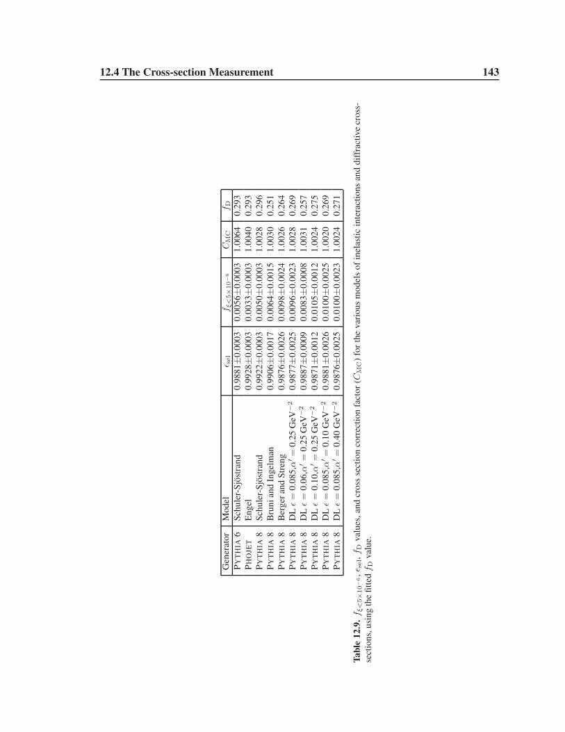
12.4 The Cross-section Measurement 143
Gen
erat
or
Mo
del
ǫ sel
f ξ<
5×
10−
6C
MC
f DP
YT
HIA
6S
chu
ler-
Sjo
stra
nd
0.9
88
1±
0.0
00
30
.00
56±
0.0
00
31
.00
64
0.2
93
PH
OJE
TE
ng
el0
.99
28±
0.0
00
30
.00
33±
0.0
00
31
.00
40
0.2
93
PY
TH
IA8
Sch
ule
r-S
jost
ran
d0
.99
22±
0.0
00
30
.00
50±
0.0
00
31
.00
28
0.2
96
PY
TH
IA8
Bru
ni
and
Ing
elm
an0
.99
06±
0.0
01
70
.00
64±
0.0
01
51
.00
30
0.2
51
PY
TH
IA8
Ber
ger
and
Str
eng
0.9
87
6±
0.0
02
60
.00
98±
0.0
02
41
.00
26
0.2
64
PY
TH
IA8
DL
ǫ=
0.0
85
,α′=
0.2
5G
eV−
20
.98
77±
0.0
02
50
.00
96±
0.0
02
31
.00
28
0.2
69
PY
TH
IA8
DL
ǫ=
0.0
6,α
′=
0.2
5G
eV−
20
.98
87±
0.0
00
90
.00
83±
0.0
00
81
.00
31
0.2
57
PY
TH
IA8
DL
ǫ=
0.1
0,α
′=
0.2
5G
eV−
20
.98
71±
0.0
01
20
.01
05±
0.0
01
21
.00
24
0.2
75
PY
TH
IA8
DL
ǫ=
0.0
85
,α′=
0.1
0G
eV−
20
.98
81±
0.0
02
60
.01
00±
0.0
02
51
.00
20
0.2
69
PY
TH
IA8
DL
ǫ=
0.0
85
,α′=
0.4
0G
eV−
20
.98
76±
0.0
02
50
.01
00±
0.0
02
31
.00
24
0.2
71
Ta
ble
12
.9.f ξ
<5×
10−
6,ǫ s
el,
f Dval
ues
,an
dcr
oss
sect
ion
corr
ecti
on
fact
or
(CM
C)
for
the
var
iou
sm
od
els
of
inel
asti
cin
tera
ctio
ns
and
dif
frac
tive
cro
ss-
sect
ion
s,u
sin
gth
efi
tted
f Dval
ue.

12.4 The Cross-section Measurement 144
σ(ξ > 5 × 10⁻⁶) [mb]
ATLAS Data 2010 60.33± 2.10(exp.)Schuler and Sjostrand 66.4PHOJET 74.2Ryskin et al. 51.8 − 56.2
σ(ξ > m2p/s) [mb]
ATLAS Data 2010 69.4 ± 2.4(exp.) ± 6.9(extr.)Schuler and Sjostrand 71.5PHOJET 77.3Block and Halzen 69 ± 1.3Ryskin et al. 65.2 − 67.1Gotsman et al. 68Achilli et al. 60 − 75
Table 12.10. Measurement and theoretical predictions of the inelastic cross-section for the restricted kine-
matic range, ξ > 5× 10⁻⁶, and for the full kinematic range, ξ > m2p/s. The experimental uncertainty (exp.)
includes the statistical, systematic and luminosity uncertainties. The extrapolation uncertainty (extr.) only
applies to the full kinematic range and is listed separately.
is the Engel-based PHOJET. The agreement between the result and the Schuler-Sjojstrand
prediction improves in the extrapolation because the DL model is used for the extrapolation
factor instead of the Schuler-Sjojstrand correction factor.
It should be noted that because the primary measurement is mostly independent of
the models, the extrapolation uncertainty can be reduced in the future when more data is
available on diffractive cross-sections at low ξ. For example, preliminary results of large
rapidity gap cross-sections up to |η| <4.9 reported in [125] indicate that PHOJET normal-
ized to a 30% relative diffractive contribution describes the data well. Future measurements
with forward proton-tagging detectors5 will greatly improve the knowledge of the single-
diffractive cross-section at low ξ [126, 127].
5The ALFA detector, a far forward proton tagging detector, is scheduled to take data in late 2011.

12.4 The Cross-section Measurement 145
[GeV]s
1 10 2103
10 410
[m
b]
ine
lσ
0
20
40
60
80
1006
> 5 x 10ξ = 7 TeV: sData 2010 6
> 5 x 10ξstrand: oSchuler and Sj6
> 5 x 10ξPHOJET (Engel et al.):
/s2
p > mξ = 7 TeV: extrap. to sData 2010
Uncertainty (incl. extrapolation)
strandoSchuler and SjBlock and Halzen 2011Achilli et al. (arXiv:1102.1949)
pp Data
Datapp
/s unless specified otherwise2
p > mξTheoretical predictions and data are shown for
ATLAS data extrapolated using Pythia implementation of DonnachieLandshoff model
ξ/dσ = 0.085 for dεwith
ATLAS
Figure 12.5. The inelastic cross-section versus√
s. The ATLAS measurement for ξ > 5 × 10⁻⁶ is shown
as the red filled circle and compared with the predictions of Schuler and Sjostrand and PHOJET for the same
phase space. Data (filled circles for pp data and unfilled circles for pp data) from several experiments are
compared with the predictions of the pp inelastic cross-section from Schuler and Sjostrand [60] (as used
by PYTHIA), by Block and Halzen [128] and by Achilli et al. [61]. An extrapolation from the measured
range of ξ > 5 × 10⁻⁶ to the full inelastic cross-section using the acceptance of 87 ± 10% is also shown
(blue filled triangle). The experimental uncertainty is indicated by the error bar while the total (including the
extrapolation uncertainty) is represented by the blue shaded area.

146
CHAPTER 13
Conclusion
In summary, this thesis details the first measurement of the proton-proton inelastic
cross-section at√s =7 TeV. The cross-section is obtained by selecting approximately 1.2
million events with at least two hits in forward scintillator counters. The luminosity of the
data sample was measured to be 20 µb−1 using a far-forward, Cherenkov light based, rela-
tive luminosity detector. The measurement is restricted to the acceptance of the scintillator
detectors, ξ > 5×10⁻⁶, where ξ = M2X/s, the invariant mass of the largest proton dissocia-
tion system in the event. This phase space fully contains non-diffractive events and accepts
over half of diffractive events. The details of the acceptance depend on the model of the
diffractive cross-section. The events are corrected for the event selection efficiency, ǫSel,
and for the fraction of events in the selected sample which have ξ < 5×10⁻⁶, fξ<5×10⁻⁶ . In
order to limit the model-dependence of the correction, the relative diffractive contribution
is measured in-situ for each of the 10 models used to generate a correction factor. The total
correction factor, including the ǫtrig, ǫsel and fξ<5×10⁻⁶ , which was derived from a model
with a single Pomeron pole with α(0) > 1,is 0.03%.
The cross-section is measured to be
σ(ξ > 5 × 10⁻⁶) = 60.33 ± 0.05(stat) ± 0.45(syst) ± 2.05(lumi) mb (13.1)
where (stat), (sys), and (lumi) are the statistical, systematic and luminosity uncertainties,
respectively. The systematic error of 0.75% is dominated by the model dependence of
ǫsel and fξ<5×10⁻⁶ . The dominant experimental uncertainty is due to the luminosity mea-
surement. It arises from the measurement of the beam currents during the van der Meer
scans which determined the luminosity calibration factor. Comparisons to the models used
by Monte Carlo generators show that the cross-section measured in the data is lower than
predicted.
In order to compare to analytic models, the measured value of the cross-section is
extrapolated to the total inelastic cross-section. The same model used to derive ǫSel and
fξ<5×10⁻⁶ is used to obtain the central value. The uncertainty on the extrapolation is as-
sessed using a variety of other models. The factor used to correct the observed cross-section

147
is 1.145±0.115, resulting in an inelastic cross-section of
σinel = 69.1 ± 2.4(stat + syst + lumi) ± 6.9(extr) mb. (13.2)
where (extr) is the uncertainty due to the extrapolation. This measurement agrees nicely
with most predictions for the cross-section at 7 TeV, but it should be noted that without a
better understanding of the differential diffractive cross-section at low ξ, the uncertainty on
the measurement is large.
The results presented here, the highest energy direct measurement of the proton-proton
inelastic cross-section, constitute a benchmark measurement for high-energy particle physics.
The measurement of the inelastic cross-section for ξ > 5 × 10⁻⁶ is well-defined with
small experimental errors and little model dependence. The extrapolation uncertainty is
at present large, but will benefit in the future from improved knowledge of the diffractive
cross-sections.

148
Bibliography
[1] Particle Data Group Collaboration, K. Nakamura et al. J. Phys. G 37 (2010)
385–401.
[2] CDF Collaboration Phys. Rev. D 50 no. 9, (Nov, 1994) 5550–5561.
[3] E710 Collaboration, N. Amos et al. Phys. Rev. Lett. 68 (1992) .
[4] E811 Collaboration, N. Amos et al. Phys. Lett. B 445 (1999) .
[5] R. J. Glauber and G. Matthiae Nucl. Phys. B 21 (1970) .
[6] T. K. Gaisser, U. P. Sukhatme, and G. B. Yodh, “Hadron cross sections at ultrahigh
energies and unitarity bounds on diffraction,” Phys. Rev. D 36 no. 5, (Sep, 1987)
1350–1357.
[7] ATLAS Collaboration, “Measurement of the Inelastic Proton-Proton Cross-Section
at√s =7 TeV with the ATLAS Detector,” arXiv:1104.0326 [hep-ex].
Submitted to Nature Communications.
[8] H. Yukawa, “On the interaction of elementary particles,” Proc. Phys. Math. Soc.
Jap. 17 (1935) 48–57.
[9] T. Regge Il Nuovo Cimento. 14 (1959) .
[10] I. Y. Pomeranchuk Soviet Physics: Journal of Experimental and Theoretical
Physics 7 (1958) .
[11] S. Donnachie, G. Dosch, P. Landshoff, and O. Nachtmann, Pomeron Physics and
QCD. Cambridge University Press, 2002.
[12] V. N. Gribov Soviet Physics: Journal of Experimental and Theoretical Physics 41
(1961) .
[13] H. B. Meyer and M. J. Teper, “Glueballs and the pomeron,” Nuclear Physics B -
Proceedings Supplements 129-130 (2004) 200 – 202. Lattice 2003.
[14] G. Jaroskiewicz and P. Landshoff Physical Review D10 (1985) .
BIBLIOGRAPHY 149
[15] E. Nagy et al. Nuclear Physics B150 (1979) .
[16] E710 Collaboration, N. Amos et al. Physics Letters B247 (1990) .
[17] J. R. Cudell, V. Ezhela, K. Kang, S. Lugovsky, and N. Tkachenko, “High-energy
forward scattering and the pomeron: Simple pole versus unitarized models,” Phys.
Rev. D 61 no. 3, (Jan, 2000) 034019.
[18] P.D.Collins and F. Gault Physical Review 73B (1978) .
[19] A. Donnachie and P. V. Landshoff, “Total cross sections,” Physics Letters B 296
no. 1-2, (1992) 227 – 232.
[20] M. Froissart, “Asymptotic behavior and subtractions in the Mandelstam
representation,” Phys. Rev. 123 (1961) 1053–1057.
[21] A. Martin Nuovo Cimento 42 (1966) .
[22] M. Gell-Mann, “The Eightfold Way: A Theory of Strong Interaction Symmetry,”
tech. rep., DOE Technical Report, 1961.
[23] G. Zweig, “An SU3 Model for Strong Interaction Symmtery and its Breaking,”
Tech. Rep. CERN Report-8419, 1964.
[24] M. Y. Han and Y. Nambu, “Three-triplet model with double su(3) symmetry,”
Phys. Rev. 139 no. 4B, (Aug, 1965) B1006–B1010.
[25] O. Greenberg, “Spin and unitary-spin independence in a paraquark model of
baryons and mesons,” Phys. Rev. Lett. 13 (1964) 598–602.
[26] R. P. Feynman, “Very high-energy collisions of hadrons,” Phys. Rev. Lett. 23 no. 24,
(1969) 1415–1417.
[27] J. D. Bjorken, “Asymptotic sum rules at infinite momentum,” Phys. Rev. 179 no. 5,
(Mar, 1969) 1547–1553.
[28] D. J. Gross and F. Wilczek, “Asymptotically free gauge theories.,” Phys. Rev. D 8
no. 10, (Nov, 1973) 3633–3652.
[29] H. D. Politzer, “Reliable perturbative results for strong interactions?,” Phys. Rev.
Lett. 30 no. 26, (Jun, 1973) 1346–1349.
[30] J. C. Collins, D. E. Soper, and G. Sterman, “Factorization for one-loop corrections
in the drell-yan process,” Nuclear Physics B 223 no. 2, (1983) 381 – 421.
[31] J. C. Collins and D. E. Soper, “Back-to-back jets in qcd,” Nuclear Physics B 193
no. 2, (1981) 381 – 443.

BIBLIOGRAPHY 150
[32] F. Low Phys. Rev. D12 (1975) .
[33] S. Nussinov Phys. Rev. Lett. 34 (1975) .
[34] J. Gunion and D. Soper Phys. Rev. D15 (1977) .
[35] A. Donnachie and P. Landshoff Phys. Lett. B296 (1992) .
[36] H1 Collaboration, “First measurement of the deep-inelastic structure of proton
diffraction,” Physics Letters B 348 no. 3-4, (1995) 681 – 696.
[37] H1 Collaboration, C. Adloff et al., “Inclusive measurement of diffractive deep
inelastic ep scattering,” Z. Phys. C76 (1997) 613–629,
arXiv:hep-ex/9708016.
[38] The Zeus Collaboration, Chekanov et al., “Measurement of the q and energy
dependence of diffractive interactions at hera,” The European Physical Journal C -
Particles and Fields 25 (2002) 169–187.
[39] J. C. Collins, “Proof of factorization for diffractive hard scattering,” Phys. Rev. D
57 no. 5, (Mar, 1998) 3051–3056.
[40] J. C. Collins, “Erratum: Proof of factorization for diffractive hard scattering [phys.
rev. d 57, 3051 (1998)],” Phys. Rev. D 61 no. 1, (Nov, 1999) 019902.
[41] G. Ingelman and P. E. Schlein, “Jet structure in high mass diffractive scattering,”
Physics Letters B 152 no. 3-4, (1985) 256 – 260.
[42] P. Newman and F. Schilling, “Hera diffractive structure function data and parton
distributions,” in Workshop on HERA and the LHC. 2004-2005.
arXiv:hep-ex/0511.032v1 [hep-ex].
[43] A. Donnachie and P. V. Landshoff, “Total cross-sections,” Phys. Lett. B296 (1992)
227–232, hep-ph/9209205.
[44] P. Desgrolard, M. Giffon, E. Martynov, and E. Predazzi, “The additive quark model
revisited: Hadron and photon induced cross-sections,” Eur. Phys. J. C9 (1999)
623–631, arXiv:hep-ph/9811393.
[45] R. Engel Z. Phys. C66 (1995) 203–214.
[46] R. Engel and J. Ranft Phys. Rev. D54 (1996) 4246–4262.
[47] A. Capella, U. Sukhatme, T. Tran, and C. Tan, “Dual parton model,” Physics
Reports 236 (1994) 225–329.

BIBLIOGRAPHY 151
[48] R. Engel, F. W. Bopp, D. Pertermann, and J. Ranft, “Extrapolation of hadron cross
sections to supercollider energies within the two-component dual parton model,”
Phys. Rev. D 46 no. 11, (Dec, 1992) 5192–5195.
[49] H. D. I. Abarbanel, J. D. Bronzan, R. L. Sugar, and A. R. White, “Reggeon field
theory: Formulation and use,” Physics Reports 21 no. 3, (1975) 119 – 182.
[50] F. W. Bopp, R. Engel, and J. Ranft, “Rapidity Gaps and the Phojet Monte Carlo,” in
LAFEX International School of High Energy Physics. 1998.
arXiv:hep-ph/9803437.
[51] M. G. Ryskin, A. D. Martin, and V. A. Khoze, “High-energy strong interactions:
from ‘hard’ to ‘soft’,” arXiv:1102.2844 [hep-ph].
[52] E. Kuraev, L. Lipatov, and V. Fadin Sov. Phys. JETP 45 (1977) .
[53] Y. Y. Balitsky and V. Fadin Sov. J. Nucl. Phys. 28 (1978) .
[54] M. Block, “Hadronic forward scattering: Predictions for the large hadron collider
and cosmic rays,” Physics Reports 436 no. 3-6, (2006) 71 – 215.
[55] M. M. Block and R. N. Cahn, “High-Energy p anti-p and p p Forward Elastic
Scattering and Total Cross-Sections,” Rev. Mod. Phys. 57 (1985) 563.
[56] CDF Collaboration, F. Abe et al. Phys. Rev. D 50 (1994) .
[57] A. Donnachie and P. V. Landshoff, “New data and the hard pomeron,” Phys. Lett.
B518 (2001) 63–71, arXiv:hep-ph/0105088.
[58] A. Donnachie and P. V. Landshoff, “Does the hard pomeron obey Regge
factorization?,” Phys. Lett. B595 (2004) 393–399, hep-ph/0402081.
[59] A. M. Mueller, “O(2, 1) analysis of single-particle spectra at high energy,” Phys.
Rev. D 2 no. 12, (Dec, 1970) 2963–2968.
[60] G. A. Schuler and T. Sjostrand, “Hadronic diffractive cross sections and the rise of
the total cross section,” Phys. Rev. D 49 no. 5, (Mar, 1994) 2257–2267.
[61] A. Achilli et al., “Total and inelastic cross-sections at LHC at CM energy of 7 TeV
and beyond,” arXiv:1102.1949 [hep-ph].
[62] E. Berger, , et al., “Diffractive hard scattering,” Nucl. Phys. B286 (1987) .
[63] K. Streng, “Hard QCD scatterings in diffractive reactions at HERA,” Tech. Rep.
CERN-TH-4949, CERN, 1988.

BIBLIOGRAPHY 152
[64] P. Bruni and G. Ingelman, “Diffractive W and Z production at colliders and the
pomeron parton content,” Phys. Lett. B311 (1993) .
[65] T. Sjostrand, S. Mrenna, and P. Skands, “Pythia 6.4 physics and manual,” JHEP 05
(2006) 026.
[66] T. Sjostrand, S. Mrenna, and P. Skands, “Pythia version 8.135,” Comput. Phys.
Commun. 178 (2008) 852–867.
[67] B. Andersson, G. Gustafson, G. Ingelman, and T. Sjostrand, “Parton fragmentation
and string dynamics,” Physics Reports 97 no. 2-3, (1983) 31 – 145.
[68] S. Navin, “Diffraction in Pythia.” 2010. arXiv:1004.0384 [hep-ph].
[69] V. Gribov, “A reggeon diagram techinque,” Sov. Phys. JETP 26 (1968) .
[70] ATLAS Collaboration, “Charged-particle multiplicities in pp interactions measured
with the ATLAS detector at the LHC,” New J. Phys. (2010) , arXiv:1012.5104
[hep-ex].
[71] ATLAS Collaboration, “ATLAS Monte Carlo Tunes for MC09.”.
ATLAS-PHYS-PUB-2010-002, http://cdsweb.cern.ch/record/1247375.
[72] P. Skands, “The Perugia Tunes.” 2009. arXiv:0905.3418 [hep-ph].
[73] R. D. Field, “Min-bias and the underlying event at the Tevatron and the LHC.”
2002. Talk presented at the Fermilab MC Tuning Workshop.
[74] S. van der Meer Tech. Rep. CERN-ISR-PO-68-31, CERN, 1968.
[75] ATLAS Collaboration, “Updated Luminosity Determination in pp Collisions at√s = 7 TeV using the ATLAS Detector.”. ATLAS-CONF-2011-011;
http://cdsweb.cern.ch/record/1334563.
[76] L. Evans, (ed.), P. Bryant, (ed.), “LHC Machine,” JINST 3 (2008) S08001.
[77] E. Eichten, I. Hinchliffe, K. Lane, and C. Quigg, “Supercollider physics,” Rev.
Mod. Phys. 56 no. 4, (Oct, 1984) 579–707.
[78] M. Bajko et al., “Report of the task force on the incident of 19th september 2008 at
the lhc.,” Tech. Rep. LHC-PROJECT-Report-1168.
CERN-LHC-PROJECT-Report-1168, CERN, 2009.
[79] “CERN-DI-0812015, http://cdsweb.cern.ch/record/1260465.”.
[80] J. Blewett, “200 TeV Intersecting Storage Accelerators,” in 8th Int. Conf. on High
Energy Accel. 1971.

BIBLIOGRAPHY 153
[81] S. Myers and F. Zimmermann, “Chamonix 2010 summary report,” in Proceedings
of Chamonix 2010 Workshop on LHC Performance. 2010.
[82] S. Myers and F. Zimmermann, “Chamonix 2011 summary report,” in Proceedings
of Chamonix 2011 Workshop on LHC Performance. 2011.
[83] ATLAS Collaboration, “The ATLAS Experiment at the CERN Large Hadron
Collider,” JINST 3 (2008) S08003.
[84] G. Aad et al., “ATLAS pixel detector electronics and sensors,” JINST 3 (2008) .
[85] A. Abdesselam et al., “The barrel modules of the ATLAS semiconductor tracker,”
Nuc. Inst. Meth. 568 (2006) .
[86] The ATLAS TRT Collaboration, “The atlas trt barrel detector,” Journal of
Instrumentation 3 no. 02, (2008) P02014.
[87] The ATLAS TRT Collaboration, “The atlas trt end-cap detectors,” Journal of
Instrumentation 3 no. 10, (2008) P10003.
[88] ATLAS Collaboration, “Liquid argon calorimeter technical design report.”.
CERN-LHCC-96-41.
[89] ATLAS Collaboration, “Readiness of the atlas liquid argon calorimeter for lhc
collisions,” The European Physical Journal C - Particles and Fields 70 (2010) .
[90] B. Aubert et al., “Development and construction of large size signal electrodes for
the atlas electromagnetic calorimeter,” Nuc. Inst. Meth. 539 (2005) .
[91] ATLAS Collaboration, “Expected Performance of the ATLAS Experiment -
Detector, Trigger and Physics,” arXiv:0901.0512 [hep-ex].
[92] The Tile Calorimeter Subsystem of the ATLAS Collaboration, “Design,
construction and installation of the atlas hadronic barrel scintillator-tile
calorimeter,” Tech. Rep. ATL-TILECAL-PUB-2008-001.
ATL-COM-TILECAL-2007-019, CERN, Geneva, Nov, 2007.
[93] K. Anderson et al., “Design of the front-end analog electronics for the atlas tile
calorimeter,” Nucl. Inst. Meth 551 (2005) .
[94] T. Cornelissen et al., “Concepts, Design and Implementation of the ATLAS New
Tracking (NEWT).” 2007.
[95] R. Fruhwirth et al., “Application of Kalman Filtering to Track and Vertex Fitting,”
Nucl. Instr. Meth. A262 (1987) .

BIBLIOGRAPHY 154
[96] D. Wicke, “New Algorithm for Solving Track Ambiguities,” Tech. Rep. DELPHI,
236:93-163, 1998.
[97] H. Gray, The Charged Particle Multiplicity at Center of Mass Energies from 900
GeV to 7 TeV measured with the ATLAS Experiment at the Large Hadron Collider.
PhD thesis, California Institute of Technology, 2010.
[98] R. Duda and P. Hart, “Use of the Hough Transformation to Detect Lines and Curves
in Pictures,” Comm. ACM 15 (1972) .
[99] ATLAS Collaboration, “Performance of primary vertex reconstruction in
proton-proton collisions at√s = 7 TeV in the ATLAS experiment.”.
ATLAS-CONF-2010-069, http://cdsweb.cern.ch/record/1281344.
[100] R. Fruhwirth et al., “Adaptive Vertex Fitting,” J. Phys. G34 (2007) .
[101] ATLAS Collaboration, “The atlas inner detector commissioning and calibration,”
Eur. Phys. J. C 70 no. arXiv:1004.5293. CERN-PH-EP-2010-043, (Jun, 2010)
787–821. 34 p.
[102] ATLAS Collaboration, “ATLAS Approved Inner detector Plots.”.
https://twiki.cern.ch/twiki/bin/view/AtlasPublic/ApprovedPlotsID.
[103] W. Cleland and E. Stern, “Signal processing considerations for liquid ionization
calorimeters in a high rate environment,” Nuclear Instruments and Methods 338
no. 2-3, (1994) .
[104] E. Fullana et al., “Digital signal reconstruction in the ATLAS hadronic tile
calorimeter,” in Real Time Conference, 2005. 14th IEEE-NPSS. 2005.
[105] ATLAS Collaboration, “Performance of the Minimum Bias Trigger in p-p
Collisions at√s = 7 TeV.” 2010. ATLAS-CONF-2010-068;
http://cdsweb.cern.ch/record/1281343.
[106] M. Tylmad et al., “Pulse Shapes for Signal Reconstruction in the ATLS Tile
Calorimeter,” in Real Time Conference, 2009. 16th IEEE-NPSS. May, 2009.
[107] ATLAS Collaboration, “The ATLAS Simulation Infrastructure,” Eur. Phys. J. C70
(2010) 823–874, arXiv:1005.4568 [physics.ins-det].
[108] GEANT4 Collaboration, S. Agostinelli et al., “GEANT4: A simulation toolkit,”
Nucl. Instrum. Meth. A506 (2003) 250–303.
[109] ATLAS Collaboration, “Charged particle multiplicities in pp interactions at√s = 7 TeV measured with the ATLAS detector at the LHC.”.
ATLAS-CONF-2010-024; http://cdsweb.cern.ch/record/1277656.

BIBLIOGRAPHY 155
[110] R. Veness et al., “The ATLAS Beam Vacuum System,” in Proceedings of PAC09.
2009.
[111] ATLAS Collaboration, “Luminosity Determination in pp Collisions at sqrt(s)=7
TeV Using the ATLAS Detector at the LHC,” Eur.Phys.J. C71 (2011) 1630,
arXiv:1101.2185 [hep-ex].
[112] W. Herr and B. Muratori, “Concept of Luminosity,” in Proceedings CAS2003,
CERN-2006-002, p. 361. 2006.
[113] H. Burkhardt and P. Grafstrom, “Absolute Luminosity From Machine Parameters,”
Tech. Rep. LHC-PROJECT-Report-1019, CERN, 2007.
[114] ATLAS Collaboration, “Luminosity Determination Using the ATLAS Detector.”.
ATLAS-CONF-2010-060, http://cdsweb.cern.ch/record/1281333.
[115] P.Darriulat and C. Rubbia Tech. Rep. CERN Internal Document 68/340/5 SIS/si.,
CERN, 1968.
[116] ATLAS Collaboration, “Charged particle multiplicities in pp interactions at√s = 7 TeV measured with the ATLAS detector at the LHC.”.
ATLAS-CONF-2010-024, http://cdsweb.cern.ch/record/1277665.
[117] G. D’Agostini, “A Multidimensional unfolding method based on Bayes’ theorem,”
Nucl. Instr. Meth. A362 (1995) 487–498.
[118] ATLAS Collaboration, “Charged-particle multiplicities in pp interactions at√s = 900 GeV measured with the ATLAS detector at the LHC,” Physics Letters B
688 (2010) 21–42.
[119] G. Anders et al., “LHC Bunch-Current Normalization for the April-May 2010
Luminosity-Calibration Measurements,” tech. rep., CERN, 2011.
[120] J. J. Gras and M. Ludwig and P. Odier, “The 2010 lhc dc bct measurement system
and its main sources of uncertainties,” Tech. Rep. LHC-Project-Note-432 ;
CERN-LHC-Project-Note-432, CERN, 2010.
[121] ATLAS Collaboration, “Studies of Diffractive Enhanced Minimum Bias Events in
ATLAS.” 2010. ATLAS-CONF-2010-048; http://cdsweb.cern.ch/record/1281302.
[122] CMS Collaboration, “Charged particle multiplicities in pp interactions at√s = 0.9,
2.36, and 7 tev. oai:cds.cern.ch:1309522,” J. High Energy Phys. 01
no. arXiv:1011.5531. CERN-PH-EP-2010-048. CMS-QCD-10-004, (Nov, 2010)
079. 36 p.

BIBLIOGRAPHY 156
[123] ALICE Collaboration, “First proton-proton collisions at the lhc as observed with
the alice detector: measurement of the charged particle pseudorapidity density at√s = 900 gev,” Eur. Phys. J. C 65 no. arXiv:0911.5430. 1, (Dec, 2009) 111. 15 p.
[124] ALICE Collaboration, “Charged-particle multiplicity measurement in
proton-proton collisions at√s = 7 tev with alice at lhc,” Eur. Phys. J. C 68
no. arXiv:1004.3514. 3-4, (Apr, 2010) 345–354. 11 p.
[125] ATLAS Collaboration, “Rapidity gap cross-sections in pp interactions√s = 7 TeV
.”. ATLAS-CONF-2011-059, http://cdsweb.cern.ch/record/1344487.
[126] ATLAS Collaboration, ATLAS Forward Detectors for Measurement of Elastic
Scattering and Luminosity. Technical Design Report. CERN, Geneva, 2008.
[127] TOTEM Collaboration, “The totem experiment at the cern large hadron collider,”
Journal of Instrumentation 3 no. 08, (2008) S08007.
[128] M. M. Block and F. Halzen, “Forward hadronic scattering at 7 tev: An update on
predictions for the lhc,” Phys. Rev. D 83 no. 7, (2011) 077901.
[129] “LHC-PHO-1999-172.”. http://cdsweb.cern.ch/record/842530.
[130] A. Martin Phys. Rev. D80 (2009) .
[131] E. Gotsman, E. Levin, U. Maor, and J. S. Miller Eur. Phys. J. C57 (2008) .
[132] E. Gotsman, E. Levin, and U. Maor arXiv:hep-ph/10105323.
[133] M. E. Peskin and D. V. Schroeder, An Introduction To Quantum Field Theory
(Frontiers in Physics). Westview Press, 1995.

157
APPENDIX A
Mandelstam Variables
The Mandelstam variables describe the kinematics of two-body scattering, as shown in
Figure A.1. The four-vectors of the particles involved are given by P1,..,4 and they can be
combined into several lorentz invarient quantities:
s = (P1 + P2)2 (A.1)
t = (P1 − P3)2 (A.2)
u = (P1 − P4)2 (A.3)
with the relation
s+ t+ u =
4∑
i=1
m2i . (A.4)
where mi is the invariant mass of particle i. Due to energy and momentum conservation,
only two out of the three mandelstam variables are independent. Most commonly s and tare used, with s corresponding the square of the center-of-mass-energy and t correspond-
ing to the square of the momentum transfer between P1 and P3. Often t and q2 are used
interchangeably, where q2 is the momentum transfer in a more complicated interaction than
2→2. In the case of hadron-hadron scattering s is the center-of-mass of the two particle,
or equivalently, the two beams of particles in the case of colliding beams. In calculating
partonic cross-sections s is used, where s is the center of mass in the parton scattering
frame.

158
1P
2P
3P
4P
Figure A.1. Two-to-two scattering process. Pi denotes the four-momentum of particle i.

159
APPENDIX B
The Optical Theorem
The optical theorem is a useful property of the scattering matrix which relates the for-
ward elastic scattering amplitude to the total cross-section. Let S be the scattering matrix,
i be the initial state, and f be the final state. The probability to be in f given i is given by
Pfi = |〈f |S|i〉|2 (B.1)
where f has the property∑
f
|f〉〈f | = 1 (B.2)
which is simply the statement that f covers all possible final states. Additionally, the
probability to end up is some final state must be unity, therefore
1 =∑
f
|〈f |S|i〉|2 (B.3)
=∑
f
〈i|S†|f〉〈f |S|i〉 (B.4)
= 〈i|S†S|i〉. (B.5)
which is to say that S is unitary. It follows that
δij = 〈j|S † S|i〉 (B.6)
=∑
f
〈j|S † |f〉〈f |S|i〉 (B.7)
for orthonormal states i and j. Let’s assume a two-body initial state i with particles with
four-momenta k1 and k2 and a final state f with an arbitrary number of particles, n. Then
we can define a transition matrix, T such that S = 1 + iT and it follows that
〈f |S|i〉 = 〈k′1k′2 · · · k′n|S|k1k2〉 (B.8)
= δif + i(2π)4δ4(P f − P i)〈f |T |i〉 (B.9)
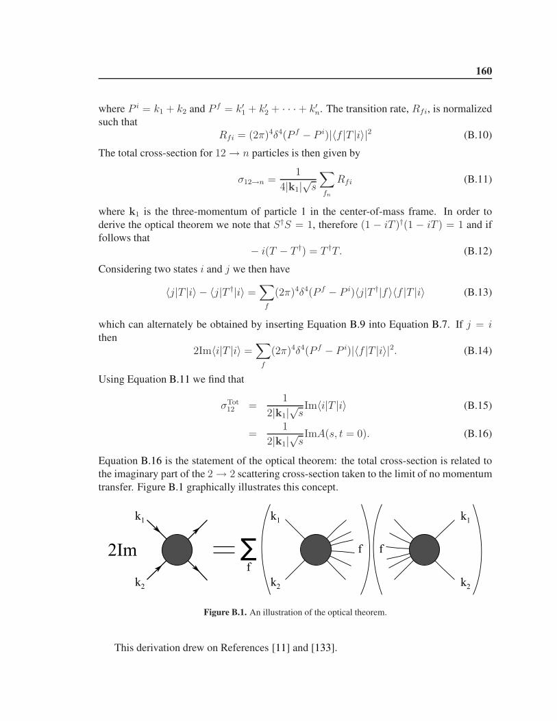
160
where P i = k1 + k2 and P f = k′1 + k′2 + · · · + k′n. The transition rate, Rfi, is normalized
such that
Rfi = (2π)4δ4(P f − P i)|〈f |T |i〉|2 (B.10)
The total cross-section for 12 → n particles is then given by
σ12→n =1
4|k1|√s
∑
fn
Rfi (B.11)
where k1 is the three-momentum of particle 1 in the center-of-mass frame. In order to
derive the optical theorem we note that S†S = 1, therefore (1 − iT )†(1 − iT ) = 1 and if
follows that
− i(T − T †) = T †T. (B.12)
Considering two states i and j we then have
〈j|T |i〉 − 〈j|T †|i〉 =∑
f
(2π)4δ4(P f − P i)〈j|T †|f〉〈f |T |i〉 (B.13)
which can alternately be obtained by inserting Equation B.9 into Equation B.7. If j = ithen
2Im〈i|T |i〉 =∑
f
(2π)4δ4(P f − P i)|〈f |T |i〉|2. (B.14)
Using Equation B.11 we find that
σTot12 =
1
2|k1|√sIm〈i|T |i〉 (B.15)
=1
2|k1|√sImA(s, t = 0). (B.16)
Equation B.16 is the statement of the optical theorem: the total cross-section is related to
the imaginary part of the 2 → 2 scattering cross-section taken to the limit of no momentum
transfer. Figure B.1 graphically illustrates this concept.
2Im ∑ f
f
k1
k2
k1
k1
k2
k2
f
Figure B.1. An illustration of the optical theorem.
This derivation drew on References [11] and [133].