a mathematical proof of the existence of trends in financial time series
TRANSCRIPT

arX
iv:0
901.
1945
v1 [
q-fin
.ST
] 14
Jan
200
9 A mathematical proof of the existence oftrends in financial time series
Michel FLIESS & Cedric JOIN
INRIA-ALIEN – LIX (CNRS, UMR 7161)Ecole polytechnique, 91128 Palaiseau, France
&
INRIA-ALIEN – CRAN (CNRS, UMR 7039)Nancy-Universite, BP 239, 54506 Vandœuvre-les-Nancy, France
Keywords: Financial time series, mathematical finance, technical analysis, trends,random walks, efficient markets, forecasting, volatility,heteroscedasticity, quicklyfluctuating functions, low-pass filters, nonstandard analysis, operational calculus.
Abstract
We are settling a longstanding quarrel in quantitative finance by proving theexistence of trends in financial time series thanks to a theorem due to P. Cartierand Y. Perrin, which is expressed in the language of nonstandard analysis (Inte-gration over finite sets, F. & M. Diener (Eds):Nonstandard Analysis in Practice,Springer, 1995, pp. 195–204). Those trends, which might coexist with some al-tered random walk paradigm and efficient market hypothesis,seem neverthelessdifficult to reconcile with the celebrated Black-Scholes model. They are esti-mated via recent techniques stemming from control and signal theory. Severalquite convincing computer simulations on the forecast of various financial quan-tities are depicted. We conclude by discussing the role of probability theory.

1 Introduction
Our aim is to settle a severe and longstanding quarrel between
1. the paradigm ofrandom walks1 and the relatedefficient market hypothesis[15]which are the bread and butter of modern financial mathematics,
2. the existence oftrendswhich is the key assumption intechnical analysis.2
There are many publications questioning the existence either of trends (see,e.g.,[15, 36, 47]), of random walks (see,e.g., [31, 55]), or of the market efficiency (see,e.g., [23, 51, 55]).3
A theorem due to Cartier and Perrin [9], which is stated in thelanguage ofnonstandardanalysis,4 yields the existence of trends for time series under a very weak integrabilityassumption. The time seriesf(t) may then be decomposed as a sum
f(t) = ftrend(t) + ffluctuation(t) (1)
where
• ftrend(t) is the trend,
• ffluctuation(t) is a “quickly fluctuating” function around0.
The very “nature” of those quick fluctuations is left unknownand nothing prevents usfrom assuming thatffluctuation(t) is random and/or fractal. It implies the followingconclusion which seems to be rather unexpected in the existing literature:
The two above alternatives are not necessarily contradictory and may coexistfor a given time series.5
We nevertheless show that it might be difficult to reconcile with our setting the cele-brated Black-Scholes model [8], which is in the heart of the approach to quantitativefinance via stochastic differential equations (see,e.g., [52] and the references therein).
Consider, as usual in signal, control, and in other engineering sciences,ffluctuation(t)in Eq. (1) as an additive corrupting noise. We attenuate it,i.e., we obtain an estimationof ftrend(t) by an appropriate filtering.6 These filters
1Random walks in finance go back to the work of Bachelier [3]. They became a mainstay in the academicworld sixty years ago (see,e.g., [7, 10, 40] and the references therein) and gave rise to a huge literature (see,e.g., [52] and the references therein).
2Technical analysis (see,e.g., [4, 29, 30, 43, 44] and the references therein), orcharting, is popularamong traders and financial professionals. The notion of trends here and in the usual time series literature(see,e.g., [22, 24]) do not coincide.
3An excellent book by Lowenstein [35] is giving flesh and bloodto those hot debates.4See Sect. 2.1.5One should then define random walks and/or market efficiency “around” trends.6Some technical analysts (see,e.g., [4]) are already advocating this standpoint.

• are deduced from our approach to noises via nonstandard analysis [16], which
– is strongly connected to this work,
– led recently to many successful results in signal and in control (see thereferences in [17]),
• yields excellent numerical differentiation [39], which ishere again of utmostimportance (see also [18, 20] and the references therein forapplications in con-trol and signal).
A mathematical definition of trends and effective means for estimating them, whichwere missing until now, bear important consequences on the study of financial timeseries, which were sketched in [19]:
• The forecast of the trend is possible on a “short” time interval under the as-sumption of a lack of abrupt changes, whereas the forecast ofthe “accurate”numerical value at a given time instant is meaningless and should be abandoned.
• The fluctuations of the numerical values around the trend lead to new ways forcomputing standard deviation, skewness, and kurtosis, which may be forecastedto some extent.
• The position of the numerical values above or under the trendmay be forecastedto some extent.
The quite convincing computer simulations reported in Sect. 4 show that we are
• offering for technical analysis a sound theoretical basis (see also [14, 32]),
• on the verge of producing on-line indicators for short time trading, which areeasily implementable on computers.7
Remark 1. We utilize as in [19] the differences between the actual prices and thetrend for computing quantities like standard deviation, skewness, kurtosis. This is amajor departure from today’s literature where those quantities are obtained via re-turns and/or logarithmic returns,8 and where trends do not play any role. It mightyield a new understanding of “volatility”, and therefore a new model-free risk man-agement.9
Our paper is organized as follows. Sect. 2 proves the existence of trends, whichseem to contradict the Black-Scholes model. Sect. 3 sketches the trend estimationby mimicking [20]. Several computer simulations are depicted in Sect. 4. Sect. 5concludes by examining probability theory in finance.
7The very same mathematical tools already provided successful computer programs in control and sig-nal.
8See Sect. 2.4.9The existing literature contains of course other attempts for introducing nonparametric risk manage-
ment (see,e.g., [1]).

2 Existence of trends
2.1 Nonstandard analysis
Nonstandard analysis was discovered in the early 60’s by Robinson [50]. It vindicatesLeibniz’s ideas on “infinitely small” and “infinitely large”numbers and is based ondeep concepts and results from mathematical logic. There exists another presentationdue to Nelson [45], where the logical background is less demanding (see,e.g., [12,13, 49] for excellent introductions). Nelson’s approach [46] of probability along thoselines had a lasting influence.10 As demonstrated by Harthong [25], Lobry [33], andseveral other authors, nonstandard analysis is also a marvelous tool for clarifying in amost intuitive way questions stemming from some applied sides of science. This workis another step in that direction, like [16, 17].
2.2 Sketch of the Cartier-Perrin theorem11
2.2.1 Discrete Lebesgue measure andS-integrability
Let I be an interval ofR, with extremitiesa andb. A sequenceT = {0 = t0 <
t1 < · · · < tν = 1} is called anapproximationof I, or anear interval, if ti+1 − tiis infinitesimalfor 0 ≤ i < ν. TheLebesgue measureonT is the functionm definedon T\{b} by m(ti) = ti+1 − ti. The measure of any interval[c, d[⊂ I, c ≤ d, is itslengthd − c. The integral over[c, d[ of the functionf : I → R is the sum
∫
[c,d[
fdm =∑
t∈[c,d[
f(t)m(t)
The functionf : T → R is said to beS-integrableif, and only if, for any interval[c, d[the integral
∫
[c,d[ |f |dm is limited and, ifd − c is infinitesimal, also infinitesimal.
2.2.2 Continuity and Lebesgue integrability
The functionf is said to beS-continuousat tι ∈ T if, and only if, f(tι) ≃ f(τ)whentι ≃ τ .12 The functionf is said to bealmost continuousif, and only if, it isS-continuous onT \R, whereR is arare subset.13 We say thatf is Lebesgue integrableif, and only if, it isS-integrable and almost continuous.
10The following quotation of D. Laugwitz, which is extracted from [27], summarizes the power of non-standard analysis:Mit ublicher Mathematik kann man zwar alles gerade so gut beweisen; mit der nicht-standard Mathematik kann man es aber verstehen.
11The reference [34] contains a well written elementary presentation. Note also that the Cartier-Perrintheorem is extending previous considerations in [26, 48].
12x ≃ y means thatx − y is infinitesimal.13The setR is said to be rare [5] if, for any standard real numberα > 0, there exists an internal set
B ⊃ A such thatm(B) ≤ α.

2.2.3 Quickly fluctuating functions
A functionh : T → R is said to bequickly fluctuating, or oscillating, if, and only if,it is S-integrable and
∫
Ahdm is infinitesimal for anyquadrablesubset.14
Theorem 2.1. Let f : T → R be anS-integrable function. Then the decomposition(1) holds where
• ftrend(t) is Lebesgue integrable,
• ffluctuation(t) is quickly fluctuating.
The decomposition(1) is unique up to an infinitesimal.
ftrend(t) andffluctuation(t) are respectively called thetrendand thequick fluctuationsof f . They are unique up to an infinitesimal.
2.3 The Black-Scholes model
The well known Black-Scholes model [8], which describes theprice evolution of somestock options, is the Ito stochastic differential equation
dSt = µSt + σStdWt (2)
where
• Wt is a standard Wiener process,
• thevolatility σ and thedrift, or trend, µ are assumed to be constant.
This model and its numerous generalizations are playing a major role in financialmathematics since more than thirty years although Eq. (2) isoften severely criticized(see,e.g., [38, 54] and the references therein).The solution of Eq. (2) is thegeometric Brownian motionwhich reads
St = S0 exp
(
(µ −σ2
2)t + σWt
)
whereS0 is the initial condition. It seems most natural to consider the meanS0eµt
of St as the trend ofSt. This choice unfortunately does not agree with the followingfact: Ft = St − S0e
µt is almost surely not a quickly fluctuating function around0,i.e., the probability that|
∫ T
0 Fτdτ | > ǫ > 0, T > 0, is not “small”, when
• ǫ is “small”,
• T is neither “small” nor “large”.
14A set is quadrable [9] if its boundary is rare.

Remark 2. A rigorous treatment, which would agree with nonstandard analysis (see,e.g., [2, 6]), may be deduced from some infinitesimal time-sampling of Eq. (2), likethe Cox-Ross-Rubinstein one [11].
Remark 3. Many assumptions concerning Eq.(2) are relaxed in the literature (see,e.g., [52] and the references therein):
• µ andσ are no more constant and may be time-dependent and/orSt-dependent.
• Eq. (2) is no more driven by a Wiener process but by more complex randomprocesses which might exhibit jumps in order to deal with “extreme events”.
The conclusion reached before should not be modified,i.e., the price is not oscillatingaround its trend.
2.4 Returns
Assume that the functionf : I → R gives the prices of some financial asset. It impliesthat the values off are positive. What is usually studied in quantitative finance are thereturn
r(ti) =f(ti) − f(ti−1)
f(ti−1)(3)
and thelogarithmic return, or log-return,
r(ti) = log(f(ti)) − log(f(ti−1)) = log
(
f(ti)
f(ti−1)
)
= log (1 + r(ti)) (4)
which are defined forti ∈ T\{a}. There is a huge literature investigating the statisticalproperties of the two above returns,i.e., of the time series (3) and (4).
Remark 4. Returns and log-returns are less interesting for us since the trends of theoriginal time series are difficult to detect on them. Note moreover that the returns andlog-returns which are associated to the Black-Scholes equation (2) via some infinites-imal time-sampling [2, 6] are notS-integrable: Theorem 2.1 does not hold for thecorresponding time series(3) and (4).
Assume that the trendftrend : I → R is S-continuous att = ti. Then Eq. (1) yields
f(ti) − f(ti−1) ≃ ffluctuation(ti) − ffluctuation(ti−1)
Thus
r(ti) ≃ffluctuation(ti) − ffluctuation(ti−1)
f(ti−1)
It yields the following crucial conclusion:
The existence of trends does not preclude, but does not implyeither, the possi-bility of a fractal and/or random behavior for the returns (3) and (4) where thefast oscillating function ffluctuation(t) would be fractal and/or random.

3 Trend estimation
Consider the real-valued polynomial functionxN (t) =∑N
ν=0 x(ν)(0) tν
ν! ∈ R[t], t ≥0, of degreeN . Rewrite it in the well known notations of operational calculus (see,e.g., [56]):
XN (s) =
N∑
ν=0
x(ν)(0)
sν+1
Introduce dds
, which is sometimes called thealgebraic derivative[41, 42], and whichcorresponds in the time domain to the multiplication by−t. Multiply both sides bydα
dsα sN+1, α = 0, 1, . . . , N . The quantitiesx(ν)(0), ν = 0, 1, . . . , N , which are givenby the triangular system of linear equations, are said to belinearly identifiable(see,e.g., [17]):
dαsN+1XN
dsα=
dα
dsα
(
N∑
ν=0
x(ν)(0)sN−ν
)
(5)
The time derivatives,i.e., sµ dιXN
dsι , µ = 1, . . . , N , 0 ≤ ι ≤ N , are removed bymultiplying both sides of Eq. (5) bys−N , N > N , which are expressed in the timedomain by iterated time integrals.Consider now a real-valued analytic time function defined bythe convergent powerseriesx(t) =
∑
∞
ν=0 x(ν)(0) tν
ν! , 0 ≤ t < ρ. Approximatingx(t) by its truncated
Taylor expansionxN (t) =∑N
ν=0 x(ν)(0) tν
ν! yields as above derivatives estimates.
Remark 5. The iterated time integrals are low-pass filters which attenuate the noiseswhen viewed as in [16] as quickly fluctuating phenomena.15 See [39] for fundamentalcomputational developments, which give as a byproduct mostefficient estimations.
Remark 6. See [21] for other studies on filters and estimation in economics andfinance.
Remark 7. See [55] for another viewpoint on a model-based trend estimation.
4 Some illustrative computer simulations
Consider the Arcelor-Mittal daily stock prices from 7 July 1997 until 27 October2008.16
4.1 1 day forecast
Figures 1 and 2 present
15See [34] for an introductory presentation.16Those data are borrowed fromhttp://finance.yahoo.com/.

0 500 1000 1500 2000 2500 30000
20
40
60
80
100
120
Samples
Figure 1: 1 day forecast – Prices (red –), filtered signal (blue –), forecasted signal(black - -)
300 400 500 600 700 800 9000
2
4
6
8
10
12
14
16
18
20
Samples
Figure 2: 1 day forecast – Zoom of figure 1

• the estimation of the trend thanks to the methods of Sect. 3, with N = 2;
• a1 day forecast of the trend by employing a2nd-order Taylor expansion. It ne-cessitates the estimation of the first two trend derivativeswhich is also achievedvia the methods of Sect. 3.17
We now look at some properties of the quick fluctuationsffluctuation(t) around thetrendftrend(t) of the pricef(t) (see Eq. (1)) by computing moving averages whichcorrespond to various moments
MAk,M (t) =
∑Mτ=0(ffluctuation(τ − M) − ffluctuation)
k
M + 1
where
• k ≥ 2,
• ffluctuation is the mean offfluctuation over theM + 1 samples,18
• M = 100 samples.
The standard deviation and its1 day forecast are displayed in Figure 3. Its het-eroscedasticity is obvious.The kurtosis MA4,100(t)
MA2,100(t)2 , the skewness MA3,100(t)
MA2,100(t)3/2, and their1 day forecasts are
respectively depicted in Figures 4 and 5. They show quite clearly that the prices do notexhibit Gaussian properties19 especially when they are close to some abrupt change.
4.2 5 days forecast
A slight degradation with a5 days forecast is visible on the Figures 6 to 10.
4.3 Above or under the trend?
Estimating the first two derivatives yields a forecast of theprice position above orunder the trend. The results reported in Figures 11-12 show for 1 day (resp.5 days)ahead75.69% (resp.68.55%) for an exact prediction,3.54% (resp.3.69%) withoutany decision,20.77% (resp.27.76%) for a wrong prediction.
17Here, as in [19], forecasting is achieved without specifying a model (see also [18]).18According to Sect. 2.2ffluctuation is “small”.19Lack of spaces prevents us to look at returns and log-returns.

0 500 1000 1500 2000 2500 30000
2
4
6
8
10
12
Samples
Figure 3:1 day forecast – Standard deviation w.r.t. trend (blue –), predicted standarddeviation (black - -)
0 500 1000 1500 2000 2500 30000
5
10
15
Samples
Figure 4:1 day forecast – Kurtosis w.r.t. trend (blue –), predicted kurtosis (black - -)

0 500 1000 1500 2000 2500 3000−4
−3
−2
−1
0
1
2
3
4
Samples
Figure 5:1 day forecast – Skewness w.r.t. trend (blue –), predicted skewness (black --)
5 Conclusion: probability in quantitative finance
The following question may arise at the end of this preliminary study on trends infinancial time series:
Is it possible to improve the forecasts given here and in [19]by taking advantageof a precise probability law for the fluctuations around the trend?
Although Mandelbrot [37] has shown in a most convincing way more than forty yearsago that the Gaussian character of the price variations should be at least questioned, itdoes not seem that the numerous investigations which have been carried on since thenfor finding other probability laws with jumps and/or with “fat tails” have been able toproduce clear-cut results,i.e., results which are exploitable in practice (see,e.g., theenlightening discussions in [28, 38, 53] and the referencestherein). This shortcomingmay be due to an “ontological mistake” on uncertainty:
Let us base our argument on new advances inmodel-free control[18]. Engineersknow that obtaining the differential equations governing aconcrete plant is always amost challenging task: it is quite difficult to incorporate in those equations frictions,20
20Those frictions have nothing to do with what are calledfrictions in market theory!

0 500 1000 1500 2000 2500 30000
20
40
60
80
100
120
Samples
Figure 6: 5 days forecast – Prices (red –), filtered signal (blue –), forecasted signal(black - -)
300 400 500 600 700 800 9000
2
4
6
8
10
12
14
16
18
20
Samples
Figure 7:5 days forecast – Zoom of figure 6

0 500 1000 1500 2000 2500 30000
2
4
6
8
10
12
Samples
Figure 8:5 days forecast – Standard deviation w.r.t. trend (blue –), predicted standarddeviation (black - -)
0 500 1000 1500 2000 2500 30000
5
10
15
Samples
Figure 9:5 days forecast – Kurtosis w.r.t. trend (blue –), predicted kurtosis (black - -)

0 500 1000 1500 2000 2500 3000−4
−3
−2
−1
0
1
2
3
4
Samples
(a) Skewness of error trend (blue –), predicted skewness of error trend (black - -) (5 day ahead)
Figure 10:5 days forecast – Skewness w.r.t. trend (blue –), predicted skewness (black- -)
heating effects, ageing, etc, which might have a huge influence on the plant’s behav-ior. The tools proposed in [18] for bypassing those equations21 got already in spiteof their youth a few impressive industrial applications. This is an important gap be-tween engineering’s practice and theoretical physics where the basic principles lead toequations describing “stylized” facts. The probability laws stemming from statisticaland quantum physics can only be written down for “idealized”situations. Is it nottherefore quite naıve to wish to exhibit well defined probability laws in quantitative fi-nance, in economics and management, and in other social and psychological sciences,where the environmental world is much more involved than in any physical system?In other wordsa mathematical theory of uncertain sequences of events should notnecessarily be confused with probability theory.22 To ask if the uncertainty of a“complex” system is of probabilistic nature23 is an undecidable metaphysical ques-tion which cannot be properly answered via experimental means. It should thereforebe ignored.
21The effects of the unknown part of the plant are estimated in the model-free approach and not neglectedas in the traditional setting ofrobust control(see,e.g., [57] and the references therein).
22It does not imply of course that statistical tools should be abandoned (remember that we computed herestandard deviations, skewness, kurtosis).
23We understand by “probabilistic nature” a precise probabilistic description which satisfies some set ofaxioms like Kolmogorov’s ones.

0 500 1000 1500 2000 2500 30000
20
40
60
80
100
120
Samples
Figure 11:1 day forecast – Prices (red –), predicted trend (blue - -), predicted confi-dence interval (95%) (black –), price’s forecast higher than the predicted trend (green△) , price’s forecast lower than the predicted trend (blue▽)
Remark 8. One should not misunderstand the authors. They fully recognize the math-ematical beauty of probability theory and its numerous and exciting connections withphysics. The authors are only expressing doubts about any modeling at large in quan-titative finance, with or without probabilities.
The Cartier-Perrin theorem [9] which is decomposing a time series as a sum of a trendand a quickly fluctuating function might be
• a possible alternative to the probabilistic viewpoint,
• a useful tool for analyzing
– different time scales,
– complex behaviors, including abrupt changes,i.e., “rare” extreme eventslike financial crashes or booms, without having recourse to amodel viadifferential or difference equations.
We hope to be able to show in a near future what are the benefits not only in quanti-tative finance but also for a new approach to time series in general (see [19] for a firstdraft).

300 400 500 600 700 800 9000
2
4
6
8
10
12
14
16
18
20
Samples
Figure 12:1 day forecast – Zoom of figure 11
References
[1] Aıt-Sahalia Y., Lo A.W.Nonparametric risk management and implied risk aver-sion. J. Econometrics,9, (2000) 9–51.
[2] Albeverio S., Fenstad J.E., Hoegh-Krøhn R., Lindstrøm T. Nonstandard Methodsin Stochastic Analysis and Mathematical Physics. Academic Press, 1986.
[3] Bachelier L.Theorie de la speculation. Ann. Sci.Ecole Normale Sup. Ser. 3,17,(1900) 21–86.
[4] Bechu T., Bertrand E., Nebenzahl J.L’analyse technique(6e ed.). Economica,2008.
[5] Benoıt E.Diffusions discretes et mecanique stochastique. Prepubli. Lab. Math.J. Dieudonne, Universite de Nice, 1989.
[6] Benoıt E.Random walks and stochastic differential equations. F. & M. Diener(Eds):Nonstandard Analysis in Practice. Springer, 1995, pp. 71–90.
[7] Bernstein P.L.Capital Ideas: The Improbable Origins of Modern Wall Street.Free Press, 1992.
[8] Black F., Scholes M.The pricing of options and corporate liabilities. J. Polit.Econ.,81, (1973) 637–654.

0 500 1000 1500 2000 2500 30000
20
40
60
80
100
120
Samples
Figure 13:5 days forecast – Prices (red –), predicted trend (blue - -), predicted confi-dence interval (95%) (black –), price’s forecast higher than the predicted trend (green△) , value is forecasted as lower than predicted trend (blue▽)
[9] Cartier P., Perrin Y.Integration over finite sets. F. & M. Diener (Eds):Nonstan-dard Analysis in Practice. Springer, 1995, pp. 195–204.
[10] Cootner P.H.The Random Characters of Stock Market Prices. MIT Press, 1964.
[11] Cox J., Ross S., Rubinstein M.Option pricing: a simplified approach. J. Finan-cial Econ.,7, (1979) 229–263.
[12] Diener F., Diener M.Tutorial. F. & M. Diener (Eds):Nonstandard Analysis inPractice. Springer, 1995, pp. 1–21.
[13] Diener F., Reeb G.,Analyse non standard. Hermann, 1989.
[14] Dacorogna M.M., Gencay R., Muller U., Olsen R.B., Pictet O.V.An Introductionto High Frequency Finance. Academic Press, 2001.
[15] Fama E.F.Foundations of Finance: Portfolio Decisions and Securities Prices.Basic Books, 1976.
[16] Fliess M.Analyse non standard du bruit. C.R. Acad. Sci. Paris Ser. I,342, (2006)797–802.
300 400 500 600 700 800 9000
2
4
6
8
10
12
14
16
18
20
Samples
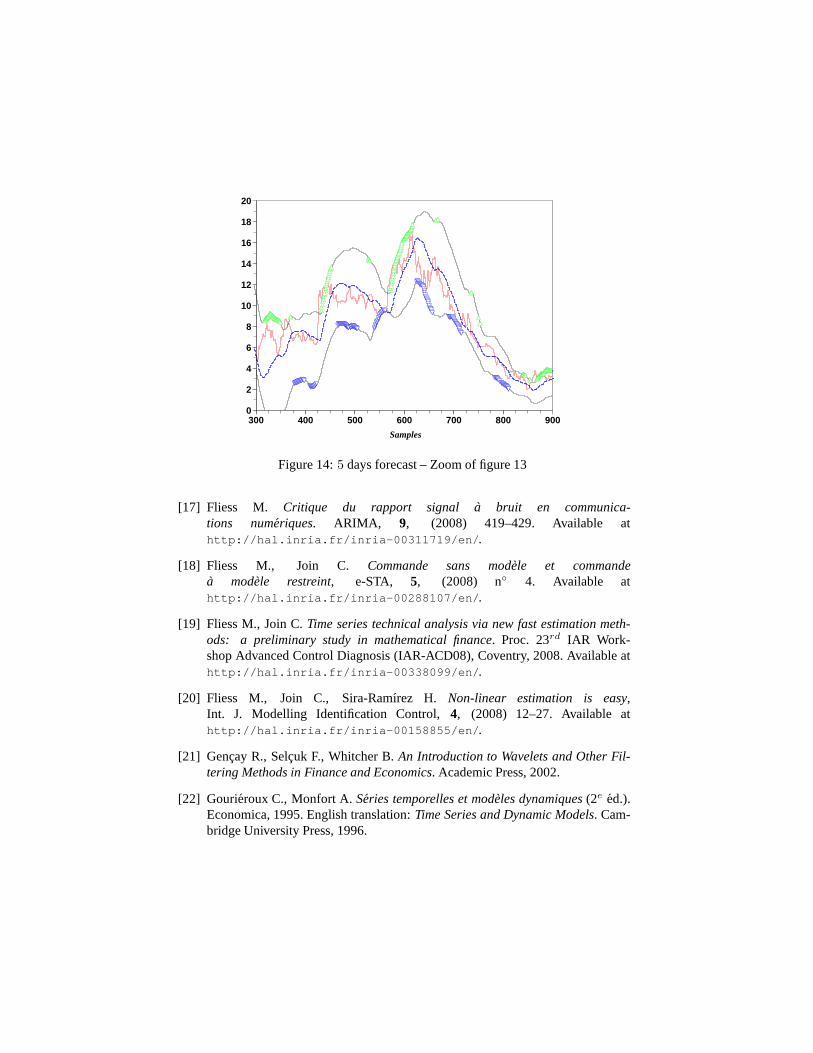
Figure 14:5 days forecast – Zoom of figure 13
[17] Fliess M. Critique du rapport signal a bruit en communica-tions numeriques. ARIMA, 9, (2008) 419–429. Available athttp://hal.inria.fr/inria-00311719/en/.
[18] Fliess M., Join C. Commande sans modele et commandea modele restreint, e-STA, 5, (2008) n◦ 4. Available athttp://hal.inria.fr/inria-00288107/en/.
[19] Fliess M., Join C.Time series technical analysis via new fast estimation meth-ods: a preliminary study in mathematical finance. Proc. 23rd IAR Work-shop Advanced Control Diagnosis (IAR-ACD08), Coventry, 2008. Available athttp://hal.inria.fr/inria-00338099/en/.
[20] Fliess M., Join C., Sira-Ramırez H.Non-linear estimation is easy,Int. J. Modelling Identification Control,4, (2008) 12–27. Available athttp://hal.inria.fr/inria-00158855/en/.
[21] Gencay R., Selcuk F., Whitcher B.An Introduction to Wavelets and Other Fil-tering Methods in Finance and Economics. Academic Press, 2002.
[22] Gourieroux C., Monfort A.Series temporelles et modeles dynamiques(2e ed.).Economica, 1995. English translation:Time Series and Dynamic Models. Cam-bridge University Press, 1996.

[23] Grossman S., Stiglitz J.On the impossibility of informationally efficient markets.Amer. Economic Rev.,70, (1980) 393–405.
[24] Hamilton J.D.Time Series Analysis. Princeton University Press, 1994.
[25] Harthong J.Le moire. Adv. Appl. Math.,2, (1981) 21–75.
[26] Harthong J.La methode de la moyennisation. M. Diener & C. Lobry (Eds):Anal-yse non standard et representation du reel. OPU & CNRS, 1985, pp. 301–308.
[27] Harthong J.Comment j’ai connu et compris Georges Reeb. L’ouvert (1994).Available athttp://moire4.u-strasbg.fr/souv/Reeb.htm.
[28] Jondeau E., Poon S.-H., Rockinger M.Financial Modeling Under Non-GaussianDistributions. Springer, 2007.
[29] Kaufman P.J.New Trading Systems and Methods(4th ed.). Wiley, 2005.
[30] Kirkpatrick C.D., Dahlquist J.R.Technical Analysis: The Complete Resource forFinancial Market Technicians. FT Press, 2006.
[31] Lo A.W., MacKinley A.C. A Non-Random Walk Down Wall Street. PrincetonUniversity Press, 2001.
[32] Lo A.W., Mamaysky H., Wang J. (2000).Foundations of technical analysis:computational algorithms, statistical inference, and empirical implementation.J. Finance,55, (2000) 1705–1765.
[33] Lobry C.La methode deselucidations successives. ARIMA, 9, (2008) 171–193.
[34] Lobry C., Sari T.Nonstandard analysis and representation of reality. Int. J. Con-trol, 81, (2008) 517–534.
[35] Lowenstein R.When Genius Failed: The Rise and Fall of Long-Term CapitalManagement. Random House, 2000.
[36] Malkiel B.G. A Random Walk Down Wall Street(revised and updated ed.). Nor-ton, 2003.
[37] Mandelbrot B.The variation of certain speculative prices. J. Business,36,(1963) 394–419.
[38] Mandelbrot B.B., Hudson R.L.The (Mis)Behavior of Markets. Basic Books,2004.
[39] Mboup M., Join C., Fliess M. Numerical differentiation with an-nihilators in noisy environment. Numer. Algorithm., (2009) DOI:10.1007/s11075-008-9236-1.

[40] Merton R.C.Continuous-Time Finance(revised ed.). Blackwell, 1992.
[41] Mikusinski J.Operational Calculus(2nd ed.), Vol. 1. PWN & Pergamon, 1983.
[42] Mikusinski J., Boehme T.Operational Calculus(2nd ed.), Vol. 2. PWN & Perg-amon, 1987.
[43] Muller T., Lindner W.Das grosse Buch der Technischen Indikatoren. AllesuberOszillatoren, Trendfolger, Zyklentechnik(9. Auflage). TM Borsenverlag AG,2007.
[44] Murphy J.J.Technical Analysis of the Financial Markets(3rd rev. ed.). New YorkInstitute of Finance, 1999.
[45] Nelson E.Internal set theory. Bull. Amer. Math. Soc.,83, (1977) 1165–1198.
[46] Nelson E.Radically Elementary Probability Theory. Princeton University Press,1987.
[47] Paulos J.A.A Mathematician Plays the Stock Market. Basic Books, 2003.
[48] Reder C.Observation macroscopique de phenomenes microscopiques. M. Di-ener & C. Lobry (Eds):Analyse non standard et representation du reel. OPU &CNRS, 1985, pp. 195–244.
[49] Robert A.Analyse non standard. Presses polytechniques romandes, 1985. En-glish translation:Nonstandard Analysis. Wiley, 1988.
[50] Robinson A.Non-standard Analysis(revised ed.). Princeton University Press,1996.
[51] Rosenberg B., Reid K., Lanstein R. (1985).Persuasive evidence of market inef-ficiency. J. Portfolio Management,13, (1985) pp. 9–17.
[52] Shreve S.J.Stochastic Calculus for Finance, I & II. Springer, 2005 & 2004.
[53] Sornette D.Why Stock Markets Crash: Critical Events in Complex FinancialSystems. Princeton University Press, 2003.
[54] Taleb N.N.Fooled by Randomness: The Hidden Role of Chance in Life and inthe Markets. Random House, 2004.
[55] Taylor S.J.Modelling Financial Time Series(2nd ed.). World Scientific, 2008.
[56] Yosida, K.Operational Calculus: A Theory of Hyperfunctions(translated fromthe Japanese). Springer, 1984.
[57] Zhou K., Doyle J.C., Glover K.Robust and Optimal Control. Prentice-Hall,1996.