J. Math. Biol.DOI 10.1007/s00285-008-0219-6 Mathematical Biology

A mathematical model for brain tumor responseto radiation therapy

R. Rockne · E. C. Alvord Jr. · J. K. Rockhill ·K. R. Swanson

Received: 12 June 2007 / Revised: 8 February 2008© Springer-Verlag 2008

Abstract Gliomas are highly invasive primary brain tumors, accounting for nearly50% of all brain tumors (Alvord and Shaw in The pathology of the aging humannervous system. Lea & Febiger, Philadelphia, pp 210–281, 1991). Their aggressivegrowth leads to short life expectancies, as well as a fairly algorithmic approach totreatment: diagnostic magnetic resonance image (MRI) followed by biopsy or surgicalresection with accompanying second MRI, external beam radiation therapy concurrentwith and followed by chemotherapy, with MRIs conducted at various times duringtreatment as prescribed by the physician. Swanson et al. (Harpold et al. in J NeuropatholExp Neurol 66:1–9, 2007) have shown that the defining and essential characteristics ofgliomas in terms of net rates of proliferation (ρ) and invasion (D) can be determinedfrom serial MRIs of individual patients. We present an extension to Swanson’s reaction-diffusion model to include the effects of radiation therapy using the classic linear-quadratic radiobiological model (Hall in Radiobiology for the radiologist. Lippincott,Philadelphia, pp 478–480, 1994) for radiation efficacy, along with an investigationof response to various therapy schedules and dose distributions on a virtual tumor(Swanson et al. in AACR annual meeting, Los Angeles, 2007).

Keywords Modeling · Radiation therapy · Glioma · Linear-quadratic ·Tumor response · Treatment fractionation

Mathematics Subject Classification (2000) 92B05

R. Rockne · E. C. Alvord Jr. · J. K. Rockhill · K. R. Swanson (B)Department of Pathology, University of Washington, Washington, USAe-mail: swanson@amath.washington.edu

123

R. Rockne et al.

1 Introduction

Gliomas are highly invasive brain tumors that spread diffusely through the brain,producing life expectancies from 6 to 12 months [1,5] for the most aggressive gradeof gliomas known as glioblastoma multiforme (GBM). In practice, an algorithmicapproach to glioma treatment includes a diagnostic magnetic resonance image (MRI)[6] followed by biopsy or surgical resection of varying extent and accompanyingsecond MRI, external beam radiation therapy (XRT) concurrent with and followed bychemotherapy, with MRIs conducted at various times during treatment as prescribedby the physician.

Radiation therapy is used as a treatment for gliomas because of the precision withwhich it targets the tumor region, and its ability to increase survival as much as twofold [7,8]. Assessing response to therapy in gliomas has historically focused on visiblechanges in gross tumor volume (GTV) as measured on MRI. Using the classic linear-quadratic model [3] for radiation efficacy, we extend Swanson’s existing glioma modelto include delivery and effect of radiation therapy. The advantage of a mathematicalmodel in this case lies in the ability to observe tumor response at any point duringtherapy, and to virtually alter the treatment schedule and dose delivery, options nototherwise available in vivo.

We present Swanson’s reaction-diffusion model [2,9–11] which describes the dif-fusion and proliferation of tumor cells in addition to the effects of precisely deliveredradiation therapy. Our model, although deterministic, is derived from stochastic firstprinciples [32]. The diffuse nature of cell motility has an implicit basis in stochastics,since we can regard the random motion and migration of cells as Brownian motion,which gives rise to the diffusion equation [12]. Additionally, radiation therapy is aninherently stochastic process since its essential mechanisms are on the atomic level:particle collision, cell death, injury and random repair can all be seen as stochasticprocesses, and are essential to the derivation of the linear-quadratic radiobiologicalmodel, [3,13–17] and therefore to the quantification of radiation therapy efficacy.Equally important is the deterministic modeling of the inherently stochastic spatialdistribution of administered radiation dose in the tumor region.

Using in vivo radiation dose distributions as reference, we investigate the spatio-temporal delivery of radiation dose, treatment response, sensitivity and recovery timefor various dose distributions and treatment fractionation schemes on a virtualtumor.

2 Model

2.1 Swanson’s glioma model

Let c = c(x, t) represent the concentration of tumor cells per mm3 at a location x attime t where the domain B (brain) is closed and bounded. What we will call Swanson’sfundamental model is a reaction-diffusion partial differential equation which describesboth the net diffusion and proliferation of tumor cells as follows:

123

A mathematical model for brain tumor response to radiation therapy

rate of changeof glioma cellconcentration

︷︸︸︷

∂c

∂t=

net dispersalof glioma cells︷ ︸︸ ︷

∇ · (D(x)∇c) +

net proliferationof glioma cells

︷︸︸︷

ρc

x ∈ B, t ≥ 0, c(x, 0) = c0, n · ∇c = 0 on ∂B (1)

where D is the spatially resolved diffusion coefficient [18,19] with units mm2/year, ρis the net rate of proliferation per year, c0 is the initial distribution of tumor cells, anda zero flux boundary condition n · ∇c = 0 which prevents cells from leaving the braindomain, B, at its boundary ∂B. Although Swanson’s model allows the diffusion coef-ficient to be a tensor to account for the complex geometry and preferential directionsfor cell migration in the brain [2], we consider here a one-dimensional, sphericallysymmetric and isotropic tissue environment where the diffusion is held constant at D.

An essential characteristic of this model is the formation of a tumor cell wave-front [20] which, in 3 dimensional spherical symmetry, asymptotically approaches aconstant velocity, v = √

2Dρ , Fisher’s approximation [12]. Although c could representany tumor population, this simple reaction-diffusion equation is an appropriate modelfor gliomas in particular for several reasons:

1. Unlike tumors in other regions of the body, the highly diffuse nature and recurrencepatterns [21] of gliomas agrees with essential properties of the model. Specifically,in as few as 7 days after tumor induction in a rat brain, glioma cells can be identifiedthroughout the central nervous system [18], analogous to the instantaneous non-zero solution of the diffusion equation on any finite domain [22]. Additionally,recurrence of glioma growth at the boundary of resection mirrors the perpetualproliferation and dispersal of any non-zero tumor cell concentration at any timepoint [23].

2. In vivo evidence suggests the observably advancing tumor front travels radially atapproximately a constant rate [24–27], and, barring treatment or physical barriersof brain anatomy, grows with spherical symmetry, aligning with Fisher’s approxi-mation [2]. Moreover, the constant velocity of untreated growth suggests that Dand ρ are characteristics intrinsic to the tumor [6,28,29].

3. The parameters D and ρ can be calculated for an individual tumor from as few astwo pre-treatment MRI’s [2], eliminating the estimation and exploration of largeparameter domains, and providing an immediately applicable metric for gliomagrowth and invasion for any given tumor in vivo.

2.2 Parameter ranges and estimation

Parameters D and ρ from Swanson’s fundamental glioma model can be computed fromas few as two pre-treatment MRI observations [2,6]. Current data from 29 tumors showa range of 6–324 mm2/year for D and 1–32 /year for ρ [2].

Despite the clinical relevance of Swanson’s fundamental model, it is only sufficientin describing untreated glioma growth. An extension of the model to include the effects

123

R. Rockne et al.

of resection and chemotherapy has been investigated [9–11,30]. However, in light ofthe pervasiveness of radiation therapy as a treatment to these tumors, an extension ofthe model to include the effects of such therapy is a natural and logical progression.

2.3 Extension to include radiation therapy

We introduce an extension to Swanson’s model of the form

rate of changeof glioma cellconcentration

︷︸︸︷

∂c

∂t=

net dispersalof glioma cells︷ ︸︸ ︷

∇ · (D(x)∇c) +

net proliferationof glioma cells

︷︸︸︷

ρc −

loss dueto therapy︷ ︸︸ ︷

R(x, t)c , (2)

where R(x, t) represents the effect of XRT at location x and time t [4]. We utilize thewidely known and accepted linear-quadratic radiobiological model [3,31,32] for thisextension, the motivation for which lies in our ability to communicate our modelingin a language familiar to our colleagues and collaborators in the medical community,as well as our belief in the relevance, versatility and robustness of the model.

Although XRT may be delivered in a variety of ways, the fundamental mechanismfor cell death is linear energy transfer, or LET [31,32]. Highly energized particlesare emitted from a radioactive source that ionizes the atoms which make up the DNA,causing lesions which can be thought of as injuries to the cell’s DNA. Cellular damageis manifested as double strand breaks (DSB) to the DNA structure. The DNA injurymakes the cell unable to reproduce itself during the next mitotic phase since transcrip-tion will be impossible.

Since LET relies on a collision between an energized radiation particle and theDNA strand of a cell, there is an inherent stochasticity in measuring the effect ofradiation, which we presume to be cell death. This manifests itself as a Poisson statis-tic [14] and provides the basis for the classic linear-quadratic (L-Q) model for radiationefficacy. The L-Q model can be derived in several ways, potentially utilizing dispa-rate assumptions about cellular response, repopulation of cells and duration of dosedelivery [13,33]. Although all have been shown to be equivalent, we prefer the deri-vation presented by Sachs et al [14], who showed that for a clonogenic cell populationN the surviving fraction N/N0 can be expressed as a sum of linear and quadraticcontributions to the log of the surviving fraction as

ln

(

N

N0

)

= −α D̃ − β D̃2 (3)

where D̃ is the total dose administered, N0 and N are cell populations before and aftertherapy, respectively, and α and β are parameters to be measured. This allows us toexpress the surviving fraction S of cells post radiotherapy as

S = exp(

−α D̃ − β D̃2)

. (4)

123

A mathematical model for brain tumor response to radiation therapy

In addition, it can be shown that cell population susceptibility based on increasedradio-sensitivity in the G2 and mitosis phases of the cell cycle can be incorporatedinto the model derivation without formal change. Therefore our implementation ofthe L-Q model need not explicitly account for cell cycle dynamics, although that is apossible avenue for further investigation.

The L-Q model by definition relates the physical dose in units of Gray (Gy) whichis the absorption of one joule (J) of radiation energy by one kilogram (kg) of matter,1Gy = J

kg to an effective dose (unitless) by the following relationship:

effective dose = α D̃ + β D̃2. (5)

In order to avoid toxic effects to normal tissue, the total dose is given in smallfractions: where n is the number of fractions, and d is the fractionated dose which isimplicitly spatially and temporally defined, so d = d(x, t) throughout. In practice,the ratio α/β is held constant at 10 Gy [3,14,16,34–37], and motivates the definitionof the following quantities, derived from the effective dose(5) :

BED = nd

(

1 + d

α/β

)

, relative effectiveness =(

1 + d

α/β

)

(6)

where BED stands for the biologically effective dose, and is a convenient measureof efficacy: total dose times its relative effectiveness [3]. The definition of BED alsoleads to the following convenient expression of survival probability,

S(α, d(x, t)) = e−αB E D . (7)

With α/β fixed, and n and d determined by the treatment schedule, the strongdependence on the single parameter α (Gy−1) is made clear. Large α implies highsusceptibility to therapy, whereas small α implies low susceptibility: we thereforeregard α as our radiation sensitivity parameter.

It should be stated that several of the well known variations on the L-Q model[13,16,38] including cellular repopulation or loss rate and effective doubling time,are included in the net growth rate ρ in Swanson’s model (1).

Now that we have established the survival probability, S, as a function of the radia-tion sensitivity parameter α and the dose distribution d = d(x, t) per fraction, (1− S)

represents the probability of cell death, and we can incorporate the effects of anyradiation treatment protocol into Swanson’s fundamental model as follows:

∂c

∂t= ∇ · (D(x)∇c) + ρc − R (α, d(x, t), t) c (8)

where

R(α, d(x, t)) ={

0, for t /∈ therapy

1 − S(α, d(x, t)), for t ∈ therapy.

123

R. Rockne et al.

with space and time domains, as well as boundary and initial conditions as statedin (1).

3 Methods

3.1 Model assumptions

For the purposes of initial exploration of the extended model, the following assump-tions are made: in addition to the central assumption of isotropic spherical symmetryD(x) = D, our model assumes no effect of central or peripheral necrosis (cell deathnot already included in the net proliferation rate ρ) on available space in the domainfor growing tumor cells, or the direct induction or deceleration of cell diffusion orproliferation due to XRT. All effects of radiation on tumor cell concentration are ins-tantaneous and deterministic, all cells are equally susceptible and likely to be killedby radiation as prescribed by the cell kill (1 − S) (7), and no delayed or otherwisetoxic effects of radiation are considered.

3.2 Non-dimensionalization and numerical algorithm

The model (8) is non-dimensionalized in one-dimension for computational conve-nience in the following way: introduce the non-dimensional quantities x = x/L ,t = ρt , c = (

cL3)

/c0 where L is the dimensional length of the computational domain,and c0 represents the initial number of tumor cells, which has no net effect on the sca-ling and is therefore arbitrary. This yields the following

ct = D∗∇2c − R∗ (

α, d( x, t ), t)

c

where, R∗ (

α, d(x, t), t) ≡

{

1, for t /∈ therapy

ζ(α, d( x, t ), t ), for t ∈ therapy.(9)

D∗ = D/(ρL2) and ζ(α, d(x, t), t) = (1 − S(α, d(x, t)))/ρ with scaled domains,initial and boundary conditions as previously stated and as in (1). All dimensionalunits are in the context of mm and years.

Model solutions are obtained using the one-dimensional discretization method ofSkeel and Berzins [39] implemented in MATLAB. The algorithm utilizes a variationon a finite-element method which is second order accurate in both space and time,resulting in spatial resolution comparable with the most highly resolved MRIs, at 1mm3. Clearly then, our measurement of tumor growth and response to therapy dependon the resolution of our spatial mesh, which need be no larger than what is measurableon MRI, therefore we take L = 200 mm, �x = 10−3 mm, and �t = 1 day. Moreover,we take n = 1 in the formulation of the BED in order to consider the dose deliveryand effect as a single, instantaneous event.

123

A mathematical model for brain tumor response to radiation therapy

Fig. 1 T1Gd and T2-weighted MRI images of a patient diagnosed with glioblastoma multiforme (GBM)

3.3 Initial condition

The extended, non-dimensional model (9) assumes an initial tumor concentrationnormally distributed as follows:

c ( x, 0) = L3e−100x2(10)

where L is the length of the dimensional computational domain. The virtual tumoris allowed to grow until it reaches a specific size, corresponding to a radius between10–20 mm, at which point radiation therapy is simulated. After the simulated therapyis completed, the tumor continues to grow for 100 additional days, at which point thesimulation is completed.

3.4 MRI thresholds of detection

Clinical observation of glioma growth and progression relies primarily on MRI [6].Swanson’s model and analysis currently utilize gadolinium enhanced T1-weighted(T1Gd) and T2-weighted MRI imaging modalities. T1Gd images abnormally leakyvasculature within the tumor, outlining the bulk of the lesion. T2-weighted MRI cap-tures edema as well as isolated tumor cells at a much lower threshold. Roughly spea-king, the T1Gd MRI reveals the tumor mass, and the T2 the tumor’s spread andassociated swelling (edema), or clinically observable boundary (Fig. 1). Although theT1Gd abnormality outlines the neovasculature, and is thought to represent the bulktumor mass, it is also potentially a poor indicator of response, as XRT damage may notcause rapid shrinkage of the abnormality. All clinical imaging modalities are limitedby thresholds of detection, though it is well known that glioma cells infiltrate throu-ghout the central nervous system well beyond any imaging abnormality [8]. Swanson’s

123

R. Rockne et al.

model is able to act as an idealized imaging technique, allowing visualization of gliomacell concentration beyond what is visible on MRI.

3.5 Radiation dose delivery and distribution

Although our model allows for any imaginable treatment schedule or dose distribution,we define the standard treatment to be the current University of Washington MedicalCenter radiation protocol: 7 weeks of treatment, using a 5 days on, 2 days off schedule(to allow for weekends) delivering 1.8 Gy to the T2 enhancing region plus a 25 mmmargin for 28 days, followed by 1.8 Gy to the T1Gd enhancing tumor region plus a20 mm margin for the remaining 6 days, yielding 61.2 Gy total max dose to the tumorbed. The region and duration of the final 6 days is considered the boost time (BT) andboost region (BR), respectively. For simplicity, all treatment simulations are assumedto begin on a Monday so that 5 consecutive days of therapy can be applied beforethe 2 day rest period is implemented. The addition of the BT and BR make our dosedistribution a function of time as well as space, so that d = d(x, t).

Days in therapy (DIT) is defined to be the duration of the therapy regimen, whereasdays of treatment (DOT) is defined to be the number of days in which XRT was actuallyadministered. For example, DIT = 35 days implies DOT = 25. In the case whereDIT is not divisible by 7, the DOT is rounded to the next integer [40]. We considerDIT as individual, independent and instantaneous events each occurring on the dayof treatment. In reality, treatment lasts several minutes each day. This assumption isconsistent with the many derivations of the L-Q model, and poses no unnecessary orextraordinary abstraction from the mechanisms modeled.

In clinical practice, radiation dose is designed and delivered in a full 3-dimensionalenvironment. Using 2-dimensional cross-sections of actual 3-dimensional dose distrib-ution maps, with additional guidance from radiation oncologist Jason Rockhill, one-dimensional dose distributions were created for use in simulations using nine fixedreference points (Fig. 2) as follows: the target dose is fixed at the tumor center, withfive points of random variation not to exceed 5% of the target dose between theorigin and enhancement boundary, with 5% of the maximum dose fixed 15 mm beyondthe enhancement boundary with margin, which determines the gradient of the doseboundary. To maintain a realistic, non-zero dose throughout the brain, we fix the doseto be zero only at the far boundary of the one dimensional domain. These points arethen interpolated with a spline interpolation algorithm, guaranteeing the smoothnessand differentiability of the dose function d(x, t).

3.6 Radiation dose fractionation

Clinically, radiation dose is delivered with the intent of maximizing (tumor) effectwhile at the same time minimizing (normal tissue) toxicity. This often leads to dailydosages of between 1 and 2.5 Gy. Hyper- and hypo-fractionation of the standard doseinvolve decreasing the incremental dose amount with an increase in frequency or viceversa, respectively [41,42]. Although thresholds for radiation toxicity and radiation-induced necrosis exist in clinical practice [43], we investigate the effects of accelerated

123

A mathematical model for brain tumor response to radiation therapy

Fig. 2 a Two-dimensional crosssection of actual dosedistribution for a patient with aGBM. Enhancement margin isnonuniform in order to avoidhigh doses of radiation to thebrain stem. b One-dimensionaldose distribution created with aspline interpolation of ninereference points. c Cumulativedose distribution showingenhancement region plus marginfor initial and boost phases ofdose delivery for the standardtreatment scheme

0 2 4 6 8 100

0.2

0.4

0.6

0.8

1

1.2

1.4

1.6

1.8

2

Radius (cm)

Dos

e (G

y)

Interpolated DoseFixed points

0 2 4 6 8 100

10

20

30

40

50

60

70

Radial Distance (cm)

Cum

ulat

ive

Dos

e (G

y)

Total Dose (Gy)T2+2.5cm (28 days)T1Gd+2cm (6 days)

T2 + 2.5cm

Boost

T1Gd + 2cm

a

b

c

or decelerated treatment on a virtual tumor, ignoring the thresholds of toxicity. Thisassumption is not grossly negligent, as current treatment practices such as gamma-knife [44] deliver a whole course (>50 Gy) of radiation treatment in a single dose with

123

R. Rockne et al.

the conscious trade off of cell kill for tangential toxicity-albeit the dose distributionfor gamma-knife is tailored much more closely to the enhancing region with a 50%decrease in dose magnitude over 2 mm typically attained, unlike the above, for whicha 50% decrease in dose magnitude spans as much as 10 mm.

4 Results

We simulate the growth and treatment of a virtual tumor under a variety of treatmentschedules and dose distributions as well as investigate the differences in responseusing different metrics. We characterize the virtual tumor with parameter values asfollows: D = 1.43 cm2/year, ρ = 16.25 /year, which serve as representative meansof published ranges [2].

4.1 Estimating radiation sensitivity

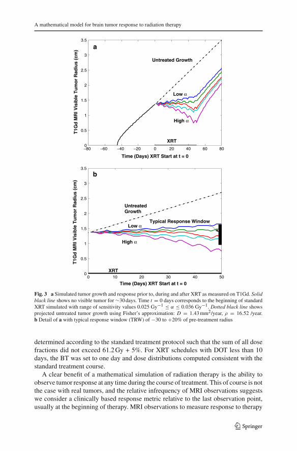
The National Cancer Institute determines tumor response to treatment using the Res-ponse Evaluation Criteria in Solid Tumors (RECIST) [45] as follows: disappearanceof all target lesions, complete response (CR), 30% decrease in pre-treatment diame-ter, partial response (PR), 20% increase in pre-treatment diameter progressive disease(PD) and small changes that do not meet the above criteria stable disease (SD). Thesymmetry of our simulations allow us to consider the RECIST criteria in the contextof radial progression of the tumor rather than diameter. Due to their significant resis-tance to radiotherapy and aggressive growth, glioma radiation response is generallyclassified as PD to PR, with response measured on T1Gd; accordingly, we define thetypical response window (TRW) as 30% decrease to 20% increase in pre-treatmentradius immediately after therapy. Given this rather coarse but nevertheless contem-porary and pragmatic view of treatment response, we can establish a realistic rangefor our radiation sensitivity parameter, α, for the virtual tumor. Using an iterativeapproach with a fixed incremental change in α, we simulated a standard courseof XRT on the virtual tumor for a large set of α values. The TRW restricts therange of reasonable radiation sensitivities to 0.025 Gy−1 ≤ α ≤ 0.033 Gy−1,well within published ranges calculated for gliomas [37,46] (Fig. 3). Although thefigure may suggest a linear relationship between α and T1Gd radius at the endof therapy, additional simulations reveal a highly non-linear pattern for changes inα, D or ρ.

The following simulations were performed with α = 0.0305 Gy−1, resulting in ∼25% decrease in pre-treatment radius for the standard XRT schedule, an optimisticand above average response to treatment.

4.2 Treatment schedule and fractionation

Several dose fractionation schemes were simulated based on the number of fractionsper day (FPD) and total DOT in intervals of 1–4 FPD and 1, 5, 10, 15, 40 DOT(Table 1) and 1, 5, 15–45 DOT (Fig. 4), respectively [41,42,47,48]. The maximumregional total dose was held constant at 61.2 Gy, with per fraction dose distributions

123

A mathematical model for brain tumor response to radiation therapy

−80 −60 −40 −20 0 20 40 60 800

0.5

1

1.5

2

2.5

3

3.5

Time (Days) XRT Start at t = 0

T1G

d M

RI V

isib

le T

um

or

Rad

ius

(cm

)

Low α

High α

XRT

Untreated Growth

0 10 20 30 40 500

0.5

1

1.5

2

2.5

3

3.5

Time (Days) XRT Start at t = 0

T1G

d M

RI V

isib

le T

um

or

Rad

ius

(cm

)

UntreatedGrowth

High α

Low αTypical Response Window

XRT

a

b

Fig. 3 a Simulated tumor growth and response prior to, during and after XRT as measured on T1Gd. Solidblack line shows no visible tumor for ∼30 days. Time t = 0 days corresponds to the beginning of standardXRT simulated with range of sensitivity values 0.025 Gy−1 ≤ α ≤ 0.036 Gy−1. Dotted black line showsprojected untreated tumor growth using Fisher’s approximation: D = 1.43 mm2/year, ρ = 16.52 /year.b Detail of a with typical response window (TRW) of −30 to +20% of pre-treatment radius

determined according to the standard treatment protocol such that the sum of all dosefractions did not exceed 61.2 Gy + 5%. For XRT schedules with DOT less than 10days, the BT was set to one day and dose distributions computed consistent with thestandard treatment course.

A clear benefit of a mathematical simulation of radiation therapy is the ability toobserve tumor response at any time during the course of treatment. This of course is notthe case with real tumors, and the relative infrequency of MRI observations suggestswe consider a clinically based response metric relative to the last observation point,usually at the beginning of therapy. MRI observations to measure response to therapy

123

R. Rockne et al.

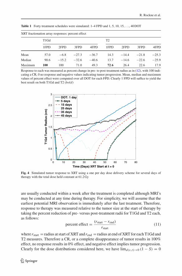
Table 1 Forty treatment schedules were simulated: 1–4 FPD and 1, 5, 10, 15, . . ., 40 DOT

XRT fractionation array responses: percent effect

T1Gd T2

1FPD 2FPD 3FPD 4FPD 1FPD 2FPD 3FPD 4FPD

Mean 57.0 −6.8 −27.3 −36.7 14.3 −14.4 −21.8 −25.3

Median 90.6 −15.2 −32.6 −40.6 13.7 −14.6 −22.6 −25.9

Maximum 100 100 71.0 49.3 72.6 26.4 22.6 17.9

Response to each was measured as percent change in pre- to post-treatment radius as in (12), with 100 indi-cating a CR, 0 no response and negative values indicating tumor progression. Mean, median and maximumvalues of percent effect were computed over all DOT for each FPD. Clearly 1 FPD will suffice to yield thebest result on both T1Gd and T2 (bold)

0 10 20 30 40 50 60 70 800

0.5

1

1.5

2

2.5

3

Time (Days) XRT Start at t = 0

T1G

d T

um

or

Rad

ius

(cm

)

DOT: 1 day5 days15 days25 days35 days45 days

Fig. 4 Simulated tumor response to XRT using a one per day dose delivery scheme for several days oftherapy with the total dose held constant at 61.2 Gy

are usually conducted within a week after the treatment is completed although MRI’smay be conducted at any time during therapy. For simplicity, we will assume that theearliest potential MRI observation is immediately after the last treatment. Therefore,response to therapy was measured relative to the tumor size at the start of therapy bytaking the percent reduction of pre- versus post-treatment radii for T1Gd and T2 each,as follows:

percent effect = (rstart − rend)

rstart(11)

where rstart = radius at start of XRT and rend = radius at end of XRT for each T1Gd andT2 measures. Therefore a CR, or a complete disappearance of tumor results in 100%effect, no response results in 0% effect, and negative effect implies tumor progression.Clearly for the dose distributions considered here, we have limd(x,t)→0 (1 − S) = 0

123

A mathematical model for brain tumor response to radiation therapy

Table 2 Forty treatment schedules were simulated using two different dose distribution techniques: 1–4FPD and 1, 5, 10, 15, . . ., 40 DOT, equal fractions and boost, respectively

XRT dose distribution responses:Net effect = percent effectequal fractions − percent effectboost

T1Gd T2

1FPD 2FPD 3FPD 4FPD 1FPD 2FPD 3FPD 4FPD

Mean 0.1 0.1 −0.1 0.1 0.4 −0.4 −0.3 −0.4

Median 0 0 0 0 0 −0.5 0 0

Maximum 13.0 2.9 2.9 1.5 3.8 0.9 0 0

Minimum −10.1 −1.5 −2.9 −1.5 −1.9 −0.9 −0.9 −0.9

Net effect quantifies the difference in effect between responses and the dose distribution techniques for eachtreatment. Mean, median, maximum and minimum values were computed over all DOT for each FPD. Thewidest range of values comes from the 1 FPD regimen, although comparisons across mean and medianssuggest very little difference between boost and equal fractions efficacy in general

for any fixed x and t , so we expect the response to hyper-fractionation to go to zeroas the number of fractions increase, leading to decreased response per fraction andtherefore a decrease in overall response. Conversely, as dose increases, (1 − S) → 1,we expect a large per fraction response and, therefore, an increase in overall response.Figure 4 reveals a wide range of responses even within the conventional single doseper day regimen, with 12.2 Gy daily for 5 days giving the best result in this simulation,and results of simulations involving all 40 treatment schedules confirm the expectationin general (Table 1).

Investigation of treatment response to schedules in the array reveals a dramaticallyincreased response on T1Gd for treatment schedules involving 1 FPD (Tables 1, 2),compared to 2, 3 or 4 FPD. T2 showed much less response across all schedules thanT1Gd, by at least 40%, consistent with the dose decreasing radially from the T1Gdabnormality for a typical dose at the T2 radius + 20 mm. The 5 DOT, 1 FPD regimenyielded the best response of 100 and 72% reduction in tumor radius on T1Gd and T2(Table 1), respectively. Only 11 of the 40 treatment schedules yielded responses withinthe TRW which included the standard therapy. The single fraction per day treatmentprovided the best response on both T1Gd and T2 by at least 23% compared to theother fractionations, excluding the near equivalence of all fractionations for treatmentdelivered on a single day, which borders on fatal radiation toxicity [3].

4.3 Radiation dose delivery

Additionally, for each treatment schedule discussed above, simulations were conduc-ted using dose distributions determined in each of two ways: equal fractions per treat-ment, and adjusted fractions based on the standard BT and BR as follows:

– Equal Fractions: a single dose distribution is formed as a sum of initial andboost phase distributions as determined by the pre-treatment tumor concentration,divided by two, such that the total dose distribution is the product of DOT andFPD and the per fraction dose distribution not to exceed 61.2 Gy + 5%. The BR is

123

R. Rockne et al.

0 10 20 30 40−100

−50

0

50

100

Days of Treatment

T1Gd XRT Effect w/ Boost

0 10 20 30 40−100

−50

0

50

100

Days of Treatment

T2 XRT Effect w/ Boost

0 10 20 30 40−100

−50

0

50

100

Days of Treatment

Per

cen

t R

edu

ctio

n in

Pre

−Tre

atm

ent

Rad

ius

T1Gd XRT Effect Equal Fractions

0 10 20 30 40−100

−50

0

50

100

Days of Treatment

T2 XRT Effect Equal Fractions

FPD: 1 2 3 4

Fig. 5 Response to therapy as measured by percent reduction in pre-treatment radius at the end of therapyas visible on T1Gd and T2 MRI for 1, 5, 10, 15,. . ., 40 DOT at each of 1–4 dose fractions per day usingtwo different dose distribution schemes: equal fractions and boost. Total dose held constant at 61.2 Gy

determined prior to therapy instead of at the beginning of the BT, and is incorporatedinto the per fraction dose distribution which does not change shape or geometry atall during treatment.

– Boost: for XRT schedules with DOT less than 10 days, the BT was set to one dayand dose distributions are computed consistent with the standard treatment course.For schedules involving 15 or more DOT, the boost time and BR were determinedat the 6th day before the end of therapy, with the total dose distribution not toexceed 61.2 Gy + 5%.

Figure 5 illustrates no qualitative difference between dose distribution schemes. Thisis significant and surprising in light of the specificity with which the boost dose dis-tribution targets the T2 region for the majority of treatment. Quantitative differencesbetween the two dose distribution schemes were taken to be the difference in percenteffect as

net effect = percent effectequal fractions − percent effectboost (12)

across all treatment schedules.

123

A mathematical model for brain tumor response to radiation therapy

0 10 20 30 400

10

20

30

40

50

60

70

80

Days of Treatment

Rec

ove

ry T

ime

(Day

s)

Equal Fractions

0 10 20 30 400

10

20

30

40

50

60

70

80

Days of Treatment

Rec

ove

ry T

ime

(Day

s)

Boost

FPD: 1234

Fig. 6 Recovery time, measured as the minimum time for which the tumor attains its pre-treatment radiusfor each of four fractions per day and 1, 5, 10, 15, . . ., 40 DOT. Recovery time was set to one day fortreatments that yielded no response

The net effect was between ±5% for all but two cases. The largest net effects inmagnitude equaled 13 and−10% for the 1 FPD regimen at 30 and 25 DOT, respectively,as measured on T1Gd. As shown in Table 2, the mean net effect for T1Gd favoredequal fractions for 3 out of 4 fractionation schemes, however, 3 out of the 4 schemesfor T2 favor boost. The median net effect is zero for all but 2 FPD on T2. This suggeststhat the differences between the dose distributions are negligible for a large majorityof the treatment schedules simulated.

4.4 Recovery time

We define recovery time (RT) to be the minimum amount of time between the start oftherapy and the time at which the tumor re-attains its pre-treatment radius as measuredon T1Gd. For treatments which yield no response, the recovery time is defined as oneday.

Recovery time was measured for all 40 treatment schedules and for both dosedistribution schemes. The recovery time falls outside of the DIT and thus a clinicallyobservable response for only 42% of the total simulated treatment schedules andfractionations in the array, including the standard treatment. Therefore in 58% of thecases, the benefit of therapy was either not clinically observable or was not beneficialat any point.

Interestingly, Fig. 6 reveals a sharp decrease in recovery time from the standardtreatment and the next DOT increment, suggesting that, although not optimal, theconventional course of therapy does avoid a drastic reduction in efficacy by only a fewtenths of a Gy in dose per treatment. Additionally, the difference in recovery time for

123

R. Rockne et al.

equal fractions versus boost dose distributions have a mean and median of zero, withmax increase of 7 days for the least effective fractionation, 4 FPD at 10 DOT.

The recovery time analysis suggests that conventional high dose hypo-fractionationtherapy, similar to gamma-knife procedures, yields the highest recovery time and, the-refore, delays progression of the tumor the most. Moreover, the conventional, dailyfractionation is vastly more effective at prolonging recovery time than multiple frac-tions per day.

5 Discussion

Although highly idealized, this simple extension of Swanson’s fundamental modelfor glioma growth and invasion [4] sheds light on the potential to incorporate existingquantifications of radiation efficacy, medical and radiological imaging into in vivotumor modeling. Investigations into fractionation schedules, dose distribution andradiation sensitivity ranges reveal the highly individualized nature of dose deliveryand non-linear response to radiation therapy. The results suggest that the conventionalcourse of treatment, involving radiation dose administered on a per day basis, is muchmore effective than several treatments per day, and that an optimal response is producedby a low frequency, high dose scheme similar to radio-surgical procedures like gamma-knife. Simulated responses to conventional treatment mirror responses expected forgliomas within published ranges, and suggest that the model and radiation sensitivityparameter α qualitatively reflect this phenomenon.

Results of simulations of the XRT schedule and fractionation array show surprisin-gly little difference between the boost and equal fraction dose distributions, particularlywith respect to T2 response. This is surprising because of the specificity with whichthe XRT dose distribution targets the T2 region during the initial phase of conventionalXRT treatment. This suggests that the BT and BR have little net effect on either theT1Gd or T2 visible portions of the tumor, consistent with recurrence patterns and theinvasive, treatment-resistant nature of gliomas. Although the T1Gd abnormality onlyindirectly represents the bulk tumor mass through its leaky neovasculature and maynot shrink to reflect the instantaneous effect of XRT on the tumor, we have used itas representative of the concentration of viable cells in that area, to remain consistentwith Swanson’s previous work [2].

A significant advantage of our model over others [15,48–50] is the relatively smallnumber of parameters and input data necessary to run the model (D, ρ and 2 pre-treatment MRIs). Our ability to calculate simulation parameters based solely on clinicalobservations yields a highly individualized and clinically relevant model which is ableto capture macroscopic tumor characteristics and which does not ignorantly simplify orovercomplicate the mechanisms modeled. Although other models [15,48–50] attempta more complicated and mechanistic approach to modeling XRT and response, noneof them can be tailored to an individual via the only clinically available metric formonitoring disease progression, namely MRI and PET imaging.

Avenues for further investigation include higher dimensional simulations withoutthe assumption of spherical symmetry, inclusion of chemo and resection therapies,quantification and minimization of radiation toxicity, incorporation of cell cycledynamics as they relate to increased radiation susceptibility, and development of a

123

A mathematical model for brain tumor response to radiation therapy

more representative measure of the number of glioma cells remaining after XRT,as well as the incorporation of PET imaging to identify molecular level resistancemechanisms such as hypoxia.

Acknowledgments The authors gratefully acknowledge the support of the McDonnell Foundation, theShaw Professorship and the Academic Pathology Fund.

References

1. Alvord EC Jr, Shaw CM (1991) Neoplasms affecting the nervous system in the elderly. In: Ducket S(ed) The pathology of the aging human nervous system. Lea & Febiger, Philadelphia, pp 210–281

2. Harpold HL, Alvord EC Jr, Swanson KR (2007) The evolution of mathematical modeling of gliomaproliferation and invasion. J Neuropathol Exp Neurol 66:1–9

3. Hall E (1994) Radiobiology for the radiologist. Lippincott, Philadelphia, pp 478–4804. Swanson KR, Rockne R, Rockhill JK, Alvord EC Jr (2007) Mathematical modeling of radiotherapy in

individual glioma patients: quantifying and predicting response to radiation therapy. In: AACR annualmeeting, Los Angeles

5. Alvord EC Jr (1995) Patterns of growth of gliomas. Am J Neuroradiol 16:1013–10176. Nelson SJ, Cha S (2003) Imaging glioblastoma multiforme. J Cancer 9:134–1457. Bloor R, Templeton AW, Quick RS (1962) Radiation therapy in the treatment of intracranial tumors.

Am J Roentgenol Radium Ther Nucl Med 87:463–4728. Chicoine M, Silbergeld D (1995) Assessment of brain tumour cell motility in vivo and in vitro.

J Neurosurg 82:615–6229. Swanson KR (1999) Mathematical modeling of the growth and control of tumors, PhD Thesis, Uni-

versity of Washington10. Woodward DE, Cook J, Tracqui P, Cruywagen GC, Murray JD, Alvord EC Jr (1996) A mathematical

model of glioma growth: the effect of extent of surgical resection. Cell Prolif 29:269–28811. Tracqui P, Cruywagen GC, Woodward DE, Bartoo GT, Murray JD, Alvord EC Jr (1995) A mathe-

matical model of glioma growth: the effect of chemotherapy on spatio-temporal growth. Cell Prolif28:17–31

12. Murray JD (2002) Mathematical biology I. An introduction, 3rd edn. Springer, New York, pp 437–46013. Carlone M, Wilkins D, Raaphorst P (2005) The modified linear-quadratic model of Guerrero and Li

can be derived from a mechanistic basis and exhibits linear-quadratic-linear behaviour. Phys Med Biol50:L9–L13 (author reply L13–L15)

14. Sachs RK, Hlatky LR, Hahnfeldt P (2001) Simple ODE models of tumor growth and anti-angiogenicor radiation treatment. Math Comp Model 33:1297–1305

15. Cunningh JR, Niederer J (1972) Mathematical-model for cellular response to radiation. Phys Med Biol17:685

16. Jones B, Dale RG (1995) Cell loss factors and the linear-quadratic model. Radiother Oncol 37:136–13917. Taylor H, Karlin S (1984) An introduction to stochastic modeling. Academic Press, Chestnut Hill18. Swanson KR, Alvord EC Jr, Murray JD (2000) A quantitative model for differential motility of gliomas

in grey and white matter. Cell Prolif 33:317–32919. Burgess PK, Kulesa PM, Murray JD, Alvord EC Jr (1997) The interaction of growth rates and diffusion

coefficients in a three-dimensional mathematical model of gliomas. J Neuropathol Exp Neurol 56:704–713

20. Swanson KR, Alvord EC Jr (2002) The concept of gliomas as a “traveling wave”: the application of amathematical model to high- and low-grade gliomas. Can J Neurol Sci 29:395

21. Alvord EC Jr (1991) Simple model of recurrent gliomas. J Neurosurg 75:337–33822. Guenther R, Lee J (1988) Partial differential equations of mathematical physics and integral equations.

Prentice Hall, Englewood Cliffs, pp 144–18723. Swanson KR, Alvord EC Jr, Murray JD (2002) Virtual brain tumours (gliomas) enhance the reality of

medical imaging and highlight inadequacies of current therapy. Brit J Cancer 86:14–1824. Capelle L, Mandonnet E, Broet P, Swanson KR, Carpentier A, Duffau H, Delattre JY (2002) Linear

growth of mean tumor diameter in WHO grade II gliomas. Neurology 58:A1325. Swanson KR, Alvord EC Jr (2002) A biomathematical and pathological analysis of an untreated

glioblastoma. In: Internatioal congress on neuropathology, Helsinki

123

R. Rockne et al.

26. Mandonnet E, Delattre JY, Tanguy ML, Swanson KR, Carpentier AF, Duffau H, Cornu P, Van Effen-terre R, Alvord EC Jr, Capelle L (2003) Continuous growth of mean tumor diameter in a subset ofgrade II gliomas. Ann Neurol 53:524–528

27. Mandonnet E, Broët P, Swanson KR, Carpentier AF, Delattre JY, Capelle L (2002) Linear growth ofmean tumor diameter in low grade gliomas. Neurology 58(Suppl 13):A13

28. Swanson KR, Rostomily RC, Alvord EC Jr (2003) Confirmation of a theoretical model describing therelative contributions of net growth and dispersal in individual infiltrating gliomas. Can J Neurol Sci30:407–434

29. Swanson KR, Alvord EC Jr (2001) A 3D quantitative model for brain tumor growth and invasion:correlation between the model and clinical behavior. Neuro Oncol 3:323

30. Swanson KR, Alvord EC Jr, Murray JD (2003) Virtual resection of gliomas: effects of location andextent of resection on recurrence. Math Comp Model 37:1177–1190

31. Tilly N, Brahme A, Carlsson J, Glimelius B (1999) Comparison of cell survival models for mixed LETradiation. Int J Radiat Biol 75:233–243

32. Sachs RK, Hahnfeld P, Brenner DJ (1997) The link between low-LET dose-response relations and theunderlying kinetics of damage production/repair/misrepair. Int J Radiat Biol 72:351–374

33. Wheldon TE, O’Donoghue JA (1990) The radiobiology of targeted radiotherapy. Int J Radiat Biol58:1–21

34. Enderling H, Anderson AR, Chaplain MA, Munro AJ, Vaidya JS (2006) Mathematical modelling ofradiotherapy strategies for early breast cancer. J Theor Biol 241:158–171

35. Jones B, Dale RG (1999) Mathematical models of tumour and normal tissue response. Acta Oncol38:883–893

36. Lee SP, Leu MY, Smathers JB, McBride WH, Parker RG, Withers HR (1995) Biologically effectivedose distribution based on the linear quadratic model and its clinical relevance. Int J Rad Oncol BiolPhys 33:375–389

37. Garcia LM, Leblanc J, Wilkins D, Raaphorst GP (2006) Fitting the linear-quadratic model to detaileddata sets for different dose ranges. Phys Med Biol 51:2813–2823

38. McAneney H, O’Rourke SF (2007) Investigation of various growth mechanisms of solid tumour growthwithin the linear-quadratic model for radiotherapy. Phys Med Biol 52:1039–1054

39. Skeel R, Berzins M (1990) A method for the spatial descretization of parabolic equations in one spacevariable. SIAM J Sci Stat Comput 11:1–32

40. Hendry JH, Bentzen SM, Dale RG, Fowler JF, Wheldon TE, Jones B, Munro AJ, Slevin NJ, RobertsonAG (1996) A modelled comparison of the effects of using different ways to compensate for missedtreatment days in radiotherapy. Clin Oncol (R Coll Radiol) 8:297–307

41. O’Donoghue JA (1997) The response of tumours with gompertzian growth characteristics to fractio-nated radiotherpay. Int J Radiat Biol 72:325–339

42. Wheldon TE, Berry I, O’Donoghue JA, Gregor A, Hann IM, Livingstone A, Russell J, Wilson L (1987)The effect on human neuroblastoma spheroids of fractionated radiation regimes calculated to be equi-valent for damage to late responding normal tissues. Eur J Cancer Clin Oncol 23:855–860

43. Abou-Jaoude W, Dale R (2004) A theoretical radiobiological assessment of the influence of radionu-clide half-life on tumor response in targeted radiotherapy when a constant kidney toxicity is maintained.Cancer Biother Radiopharm 19:308–321

44. Gerosa M, Nicolato A, Foroni R (2003) The role of gamma knife radiosurgery in the treatment ofprimary and metastatic brain tumors. Curr Opin Oncol 15:188–196

45. Padhani AR, Ollivier L (2001) The RECIST (response evaluation criteria in solid tumors) criteria:implications for diagnostic radiologists. Br J Radiol 74:983–986

46. Qi XS, Schultz CJ, Li XA (2006) An estimation of radiobiologic parameters from clinical outcomesfor radiation treatment planning of brain tumor. Int J Radiat Oncol Biol Phys 64:1570–1580

47. Wheldon TE, Deehan C, Wheldon EG, Barrett A (1998) The linear-quadratic transformation of dose-volume histograms in fractionated radiotherapy. Radiother Oncol 46:285–295

48. Ribba B, Colin T, Schnell S (2006) A multiscale mathematical model of cancer, and its use in analyzingirradiation therapies. Theor Biol Med Model 3

49. Stamatakos GS, Antipas VP, Uzunoglu NK, Dale RG (2006) A four-dimensional computer simulationmodel of the in vivo response to radiotherapy of glioblastoma multiforme: studies on the effect ofclonogenic cell density. Br J Radiol 79:389–400

50. Enderling H, Chaplain MA, Anderson AR, Vaidya JS (2007) A mathematical model of breast cancerdevelopment, local treatment and recurrence. J Theor Biol 246:245–259

123