Turkish J. Eng. Env. Sci.32 (2008) , 85 – 100.c© TUBITAK

A Mathematical Framework for Simulation of Thermal Processingof Materials: Application to Steel Quenching

Caner SIMSIRStiftung Institut fur Werkstofftechnik Badgasteiner Str. 3

28359 Bremen-GERMANYe-mail: simsir@iwt-bremen.de

Cemil Hakan GURMiddle East Technical University, Department of Metallurgical and Materials Engineering

Ankara-TURKEY

Received 03.09.2007

Abstract

During thermal processing, parts are usually subjected to continuous heating and cooling cycles duringwhich microstructural and mechanical evolutions occur simultaneously at different length and time scales.Modeling of these processes necessitates dealing with inherent complexities such as large material propertyvariations, complex couplings and domains, combined heat and mass transfer mechanisms, phase transfor-mations, and complex boundary conditions. In this study, a finite element method based mathematicalframework capable of predicting temperature history, evolution of phases and internal stresses during ther-mal processing of materials was developed. The model was integrated into the commercial FE softwareMSC.Marc r© by user subroutines. The accuracy of the model was verified by simulating the quenching ofhollow steel cylinders. Simulation results were compared with SEM observations and XRD residual stressmeasurements. According to the results, the model can effectively predict the trends in the distribution ofmicrostructure and residual stresses with remarkable accuracy.

Key words: Thermal Processing, Modeling, Simulation, Quenching, Steel

Introduction

Thermal processing of materials refers to manufac-turing and material fabrication techniques that arestrongly dependent on the thermal transport mech-anisms. With the substantial growth in new andadvanced materials like composites, ceramics, differ-ent types of polymers and glass, coatings, special-ized alloys, and semiconductor materials, thermalprocessing has become particularly important sincethe properties and characteristics of the product, aswell as the operation of the system, are largely deter-mined by heat transfer mechanisms (Jaluria, 2003).

A few important materials processing techniquesin which heat transfer plays a very important roleare listed in Table 1. The list contains both tradi-

tional processes and new or emerging methods. Inthe former category, welding, metal forming, poly-mer extrusion, casting, heat treatment, and dryingcan be included. The rest may be included in thelatter category.

The dependence of the properties of the finalproduct on the physics of the process must be clearlyunderstood so that analysis or experimentation canbe used to design processes to achieve optimum qual-ity at desired production rates. Modeling is one ofthe most crucial elements in the design and optimiza-tion of thermal materials processing systems.

Mathematical and numerical modeling of ther-mal processing of materials is a challenging task. Amodel must deal with at least one or several of thefollowing difficulties:

85

SIMSIR, GUR

Table 1. Examples of thermal processing of materials.

Process Category ExamplesSolidification Casting, continuous casting, crystal growingHeat Treatment Annealing, hardening, tempering, surface treatments, curing, bak-

ingForming Hot rolling, wire drawing, metal forming, extrusion, forging, press

forming, injection molding, thermoforming, glass blowingBonding Soldering, welding, chemical-diffusion bondingCoating Thermal spray coating, polymer coatingPowder Processing Powder metallurgy, ceramic processing, sintering, sputteringOther Composite materials processing, microgravity materials process-

ing, rapid prototyping

• The model may require dealing with highlynonlinear material properties since materialproperties usually have a pronounced variationwith temperature, stress, and concentration.

• The model may require including couplingsbetween different physical events such asheat/mass transfer, mechanical interactions,phase transformations, and chemical reactions.

• The model may require handling of multiscalecouplings due to mechanisms operating at dif-ferent length and time scales.

• The model may necessitate handling of com-plex geometries and domains since engineeringsystems for thermal processing usually involvecomplex geometries with multiple domains.

• The model may require dealing with complexboundary conditions such as highly nonlinearand moving boundary conditions.

• The model may necessitate handling of differ-ent energy sources ranging from conventionalheating to laser, induction, gas, fluid jet heat-ing/cooling.

In this study, a flexible mathematical framework forsimulation of thermal processing of materials, capa-ble of dealing with most of the above difficulties, isdeveloped and integrated into commercial finite ele-ment analysis software MSC.Marc r© by user subrou-tines. The framework has a modular structure andallows coupling of different simulation and numeri-cal solution techniques with FEM. As a case study,the model is verified by simulating the quenching ofhollow C60 steel cylinders from 830 ◦C into 20 ◦Cwater. Simulation results were compared with SEMinspection and residual stress measurements.

Mathematical Framework

Thermal processing of materials is a complex mul-tiscale and multiphysics problem. During the ther-mal processing of materials, parts are usually sub-jected to continuous heating and cooling cycles dur-ing which microstructural and mechanical evolutionsoccur simultaneously at different length scales. Eachphysical field is described by governing equations andan appropriate set of initial and boundary condi-tions. Most of those equations have a nonlinear na-ture. In addition, physical fields interact with eachother either by sharing of state variables or by cou-pling interactions. Figure 1 is a brief representationof physical fields and couplings during the thermalprocessing of materials.

Analytical solution of coupled nonlinear equa-tions is usually not possible. The rigorous treat-ment of the problem requires a coupled total thermo-mechano-microstructural theory. However, a com-monly accepted incorporation of the kinetics and ir-reversible thermodynamics of the phase transforma-tions in such a coupled theory has not been done sofar. As a remedy, a “staggered numerical solution”of the problem is suggested in this study.

The currently developed framework consists of amodular system, in which each module deals witha certain physical field and related couplings. Thesolution may involve the application of numericalmethods such as the finite difference method (FDM),finite volume method (FVM), and finite elementmethod (FEM). In this study, FEM is used for nu-merical solution of most of the physical fields suchas thermal and mechanical fields because of its widespectrum of applicability and ease of use. FDMis used for the solution of anisothermal kinetics ofphase transformations.

86

SIMSIR, GUR

PHASETRANSFORMATIONS

(METALLURGICAL FIELD)

STRDESS/STRAINEVOLUTION

(MECHANICAL FIELD)

Transformation Strains

Phase Fraction Dependent Mechanical Properties

Stress/Strain Affected Transformations

CHEMICALCOMPOSITION

HEAT TRANSFER

(THERMAL FIELD)

THERMOPHYSICALEVENTS

(Ex: Leidenfrost Effect)

FLUID FLOW

(FLUID DYNAMICS FIELD)

Ther

mal

Driv

ing

Fo

rceTherm

al StrainsPh

ase

Frac

tion

Dep

ende

nt Thermal Temperature Depentent M

echanical

Late

ntH

eat

Heat Induced byD

eformation

Figure 1. A general representation of physical fields and interactions during thermal processing of materials.

The simplest case of thermal processing of ma-terials involves coupled calculation of heat transferand microstructural evolution. This type of couplingmay be sufficient if the phase transformations are nothighly affected by stress/strain and the calculationof mechanical interactions (stresses/strains) is notimportant. However, in most industrial cases, thisassumption is not valid at all. A much more real-istic case involves the calculation of heat transfer,and microstructural and mechanical evolution. Thiscase covers many thermal treatments applied to en-gineering materials. Formulation of the mechanicalfield may involve elastic stress/strain analysis, e.g.,thermal processing of ceramics, an elastoplastic anal-ysis, e.g., heat treatment of metals and alloys, orviscoelastoplastic analysis, e.g., thermal processingof polymers, processes involving slow cooling rates.Due to its flexible and modular design, all of thesecouplings and variations may be incorporated intothe current framework with minor revisions.

Another advantage of the current framework liesin its ability to deal with multiscale treatment ofcertain phenomena such as phase transformationsand transformation plasticity since the phase trans-formation module runs on an integration point ba-sis. Lower scale simulations (mesoscopic or atom-istic) can be performed using a representative vol-ume elements (RVE) and proper scale shifting meth-ods. In addition, the current framework allows thecoupling of the heat transfer field with other phys-ical fields controlling heat transfer. For example,heat transfer from the surface is controlled by fluidflow around the component in many cases. Con-vective cooling rates are highly dependent on thefluid flow velocity, the viscosity, and the heat ca-pacity of the process medium. Computational fluiddynamics (CFD) calculations may be coupled to de-termine actual surface heat flux. A weak coupling offluid flow field with thermo-mechano-microstructuralanalysis may be created by importing the mass flow

87

SIMSIR, GUR

rate of the fluid calculated in a CFD program such asFLUENT r© and CFX r© as a function of position andtime and applying this information as the thermalboundary condition. Another example of a physicalevent controlling the heat transfer may be illustratedin induction heating of ferrous alloys, during whichmagneto-electrical heating drives the heat transfer.This kind of simulation may allow engineers to opti-mize the system to optimize the distortion, residualstress, and microstructure distribution.

Chemical composition (diffusion) field is also an-other important physical field that should be takeninto account for simulation of thermal processes dur-ing which the chemical composition is not macro-scopically homogeneous. This field involves the so-lution to Fick’s diffusion equation. This field isnot currently incorporated into the developed frame-work. Its incorporation may allow the simulation ofthermo-chemical surface treatments such as carbur-izing and nitriding of steel components.

Physical fields and coupling interactions

Heat transfer is the major driving event triggeringthe other events. Heat transfer from the surface ishighly dependent on the transfer mechanisms (con-duction, convection, and radiation), fluid flow, andthermo-physical and thermo-chemical processes oc-curring at the interface. Other important physicalevents of the thermal processing of materials arephase transformations and the generation of an in-ternal stress field due to thermal gradients and phasetransformations.

Thermal stresses are generated in the thermallyprocessed material due to large temperature gra-dients and the variation in mechanical propertieswith temperature. Varying heating/cooling ratesat different points lead to varying thermal expan-sions/contractions, which must be balanced by an in-ternal stress state. Those stresses may cause nonuni-form plastic flow when their magnitude at any pointexceeds local yield strength. On the other hand,plastic deformation causes heat generation due to in-ternal friction. However, heat induced by deforma-tion is usually negligible since plastic deformationsare relatively small (2%-3%) during thermal treat-ments.

Variation in temperature at any point in ther-mally processed material is the major driving forcefor phase transformations. Upon treatment, thethermodynamic stability of the parent phase is al-tered, which results in decomposition of the parent

phase into transformation products. The transfor-mation rate basically depends on the temperatureand the cooling/heating rate. On the other hand,there exists a heat interaction with the surround-ings during phase transformations. Phase transfor-mations that occur during quenching are exothermicand they alter the thermal field by releasing latentheat of transformation. It has been shown that ne-glecting this effect has a strong side effect on the ac-curacy of the determination of the temperature field(Denis et al., 1992).

Typically, a material undergoing a heat treat-ment is subjected to a fluctuating triaxial stressstate and small plastic strains (up to 2%-3%)due to thermal stresses and phase transformations.These strains may be due to density change, elas-tic coherency, or transformation induced plasticity(TRIP). TRIP is the significantly increased plastic-ity during a phase change. Even for an externallyapplied load for which the corresponding equivalentstress is small compared to the normal yield stress ofthe material, plastic deformation occurs. This phe-nomenon is explained by the existence of an irre-versible strain resulting from phase transformationunder stress. TRIP is currently explained by thecompetition of 2 mechanisms depending on thermo-mechanical loading conditions (Cherkaoui, 2002):

• Plastic Accommodation (Greenwood-Johnson)Mechanism: During phase transformations un-der a stress field, the interaction of the loadstress and the geometrically necessary stress toaccommodate the transformation eigenstrainresults in an irreversible strain. This pioneer-ing explanation of TRIP was given by Green-wood and Johnson (1965). This mechanismis operational for both displacive (martensitic)and reconstructive (diffusional) phase transfor-mations.

• Variant Selection (Magee) Mechanism:Martensitic transformation from FCC to BCC(and BCT) crystal structure occurs with 24possible variants, each characterized by a dis-tinct lattice orientation relationship. At themesoscopic scale, each variant is defined by atransformation strain involving a dilatational(δ) component perpendicular to the habitplane and a shear component (γ) on the habitplane. In general, only the preferred variantsare nucleated upon thermo-mechanical loadingdepending on the stress state. The earliest ob-servation of this mechanism based on variant

88

SIMSIR, GUR

selection was in the works by Patel and Cohen(1953). Later, this mechanism was called the“Magee” mechanism due to his famous studyon the importance of formation of preferredvariants in iron based alloys (Magee, 1966).

Phase transformations that occur under stressand with prior or concomitant plasticity can be con-sidered examples of ‘materials systems under drivingforces’ in which both the driving forces for transi-tion and the kinetics of the process can be alteredby mechanical interactions. The interaction of me-chanical driving forces and phase transformations de-pends both on the material and loading conditions.For example, the thermodynamics of phase trans-formations, i.e. transformation temperatures, andchemical composition of parent and product phases,is modified by the change in free energies of parentand product phases. Similarly, kinetics of transfor-mation, i.e. transformation rates, path of transfor-mation, may also be altered because of the changein the mobility of atoms due to elastic and plasticstrains. Elastic strains affect the kinetics of transfor-mation by changing the mobility of atoms by chang-ing the free volume. Plasticity alters the transportprocesses by changing the point defect concentration,providing shortcuts for diffusion via dislocation coresor by providing a nondiffusive transport mechanismwhere the atoms are convected by moving disloca-tions either geometrically or via the drag effect due todislocation/solute interaction (Embury et al., 2003).

First observations and modeling studies in thefield are focused on the effect of stress and plasticdeformation on martensitic transformations. It hasbeen observed that a uniaxial stress leads to an in-crease in Ms, whereas hydrostatic pressure and plas-tic deformation results in a decrease. However, aplastic strain of 1%-3%, which is common in ther-mal processing of metals and alloys, only causes achange of a few degrees but a stress close to theyield strength of the parent phase leads to a changeof 30-50 ◦C. Thus, for the purpose of simulation ofthermal processing, during which large stresses andsmall plastic strains are characteristic, the effect ofplastic strain on Ms may be neglected.

Formulation of thermal field

Accurate prediction of thermal history is vital forsimulation purposes and accurate results can onlybe obtained by deep understanding of the heattransfer phenomenon. The accuracy of the ther-

mal history prediction influences directly the accu-racy of phase transformation kinetics, and thermaland phase transformation stress calculations. A poorheat transfer model or inaccurate heat transfer datawill eventually result in considerable errors in thepredicted microstructure and stresses even thoughthe phase transformation and mechanical modulesare functioning perfectly.

The transient heat transfer within the materialduring thermal processing can be described mathe-matically by an appropriate form of Fourier’s heatconduction equation. Considering that the thermalfield is altered by latent heat of phase transforma-tions, the equation can be expressed in its most gen-eral form as

ρc∂T

∂t= div(λ∇T ) + Q (2.1)

where ρ, cp, and λ are the density, specific heat, andthermal conductivity of the phase mixture given as afunction of temperature, respectively. Q is the inter-nal heat source/sink term due to latent heat releasedper unit mass, which is a function of transformationrate and temperature as

Q = Lk ξk (2.2)

where L is the latent heat of transformation.Thermal properties of the phase mixture may be

approximated by a linear rule of mixture

P (T, ξk) =N∑1

Pkξk (2.3)

where P represents an average thermal property ofthe mixture, and Pk is a thermal property of the kth

constituent of the phase mixture. ξk is the volumefraction of the kth constituent.

The energy change (i.e. the temperature drop)due to adiabatic expansion and the energy due toplastic flow are also neglected. Simple estimatesshow that their contribution to heat generation rateterms is less than 1% for nearly incompressible solids(Sjostrom, 1984).

Finally, initial and boundary conditions must beset to complete the definition of the thermal prob-lem. A surface temperature dependent convectiveheat transfer boundary condition can be defined as

Φ(Ts, T∞) = h(Ts)(Ts − T∞) (2.4)

where Φ is the heat flux from the surface, which isa function of surface and the quenchant tempera-ture. h(Ts) is the surface temperature dependent

89

SIMSIR, GUR

heat transfer coefficient. Use of a surface tempera-ture dependent heat transfer coefficient permits usto incorporate the effect of different cooling rates atdifferent stages of heat treatment. Similarly, a radi-ation boundary condition can be defined as

Φ(Ts, T∞) = kBζ(T 4s − T 4

∞) (2.5)

where ζ is the emissivity of the surface and kB is theStephan-Boltzmann constant.

An insulated boundary can be specified by set-ting the heat flux to 0 by

Φ = −λ∂T

∂n= 0 (2.6)

where ∂T/∂n is the directional derivative of the tem-perature in the outer normal (n) direction.

Formulation of microstructural field

Several mathematical models have been proposed formathematical description of the isothermal transfor-mation kinetics of solid state transformations, mostof which are based on the same principles with mi-nor modifications. In these models, the transformedfraction is expressed by

ξk=

⎧⎪⎪⎪⎨⎪⎪⎪⎩

1 − exp (−bktnk) ; r = 1 (Avrami)1− (1 + bktnk)−1 ; r = 2 (Austin-

Rickett)

1− (1+ (rk−1) bkt)�

rk−1nk

�; r �= 1

(2.7)where b, n, and r are temperature dependent timecoefficient, time exponent, and saturation parame-ter, respectively. n depends on the ratio of nucleationand growth rates, whereas b depends on the absolutevalues of nucleation and growth rate. r depends onthe growth mode and the temperature, and differentchoices result in different kinetic equations. For ex-ample, the equation obtained is the Avrami equationwhen r = 1 and the Austin-Rickett equation when r= 2 (Avrami, 1939).

The Johnson-Mehl-Avrami-Kolmogorov (JMAK)equation may be corrected to account for phasetransformations that start from a phase mixture anddo not saturate to 100% as

ξk = ξok + (ξeq

k − ξok) (1 − exp (bktnk)) (2.8)

where ξo and ξeq are the initial and the equilibriumconcentrations.

Equation (2.8) can be further improved to dealwith anisothermal kinetics of phase transformations

by Scheil’s additivity principle, which was later ex-tended to solid state phase transformation by Cahn(1956) and generalized by Christian (1975). Ac-cording to Scheil’s additivity rule, if τ (ξk,T) is theisothermal time required to reach a certain trans-formed amount ξk, the same transformation amountwill be reached under anisothermal conditions whenthe following Scheil’s sum (S) equals unity (Scheil,1935):

S =

t∫0

dt

τ (ξk, T )= 1 (2.9)

This rule can be exploited in the calculation of boththe incubation times and the anisothermal kineticsof transformations. The calculation of incubationtime, as summarized in Figure 2, is straightforward;replacing τ (ξk, Ti)with isothermal incubation time(τs(Ti)) results in

S =n∑

i=1

Δtiτs(Ti)

≈ 1 (2.10)

The incubation is considered complete when S equalsunity.

After the completion of incubation, growth ki-netics is calculated, which is illustrated in Figure7. Considering the Avrami kinetic equation, a fic-titious time τ , which is dependent on the fractiontransformed up to the end of the previous time step,is calculated by

τ =(− ln (1 − ξk(t))

bk

) 1nk

(2.11)

Next, the fictitious time is incremented by time stepsize (Δt) in order to calculate a new fictitious trans-formed fraction. Using the fictitious transformedfraction, actual transformed amount is calculated by

ξt+Δtk = ξmax

k

(ξtγ − ξt

k

)(1 − exp (bk (τ + Δt)nk))

(2.12)where ξmax

k is the maximum fraction of the productphase. In the case of transformations that do notsaturate to 100% completion ξmax

p can be calculatedusing the lever rule in the equilibrium phase diagram.

90

SIMSIR, GUR

TE

MPE

RA

TU

RE

TIME

ISOTHERMALTRANSFORMATION

START CURVECOOLINGCURVE

τj+1 τj τj-1

Δτj+1

Δτj

Δτj-1

Figure 2. Schematic representation of calculation ofanisothermal incubation time from TTT dia-gram using Scheil’s additivity principle.

TE

MPE

RA

TU

RE

TIME

Tj+1

tj

Δτj+1

τj

Δτj+1

t+τ

Tjl l

TIME

ξkj

ξkj+1

Δτj+1

tj tj+1

VO

L. F

RA

CT

ION

Figure 3. Schematic representation of calculation ofanisothermal growth kinetics from isothermalkinetics by Scheil’s additivity principle.

This expression may be further improved to takeinto account the effect of stress on diffusional phasetransformations. For example, Hsu (2005) proposeda modified JMAK equation in which both the coef-ficient (b) and the exponent (n) of kinetic equationare functions of effective stress as

ξp = ξγ .(1 − exp

(−b(σ)tn(σ)

))(2.13)

b(σ) = b(0)(1 + AσB) (2.14)

n(σ) = n(0) (2.15)

where parameters A and B can only be determinedby regression of experimental data and are depen-dent on the material and phase transformation type.b(0) and n(0) can be calculated from TTT data.

Modeling the martensitic (displacive) transfor-mations Martensite is generally considered to formby a time independent transformation below Ms tem-perature. Therefore, its kinetics is essentially not in-fluenced by the cooling rate and cannot be describedby Avrami type of kinetic equations. The amount ofmartensite formed is often calculated as a function oftemperature using the law established by Koistinenand Marburger (1959),

ξm = ξγ (1 − exp (−Ω (Ms − T ))) (2.16)

where Ω is a material constant, whose value is 0.011for many steels regardless of chemical composition.

It should also be noted that Ms temperature isalso dependent on the stress state, prior to plasticdeformation. Various models have been developedfor quantitative description of the effect of stresson martensitic transformations (Inoue and Wang,1982; Loshkarev, 1986; Denis et al., 1987). Mostof them are based on modification critical tempera-tures and the Koistinen-Marburger law. Inoue (In-oue and Wang, 1985) proposed a model in which thechange in Ms (ΔMs) is a function of mean stress(σm) and the second invariant of deviatoric stresstensor (J2). According to his model, the change inMs is described as

ΔMs = Aσm + BJ1/22 (2.17)

where A and B material are dependent constantsthat can be determined experimentally.

Formulation of mechanical field

Material models that have been proposed for simu-lation of thermal processing of materials can be clas-sified into elastoplastic, elasto-viscoplastic, and uni-fied plasticity constitutive models. Almost all of theformulation of constitutive equations is based on theadditive decomposition of strain tensor. Rate inde-pendent elastoplastic models are the most frequently

91

SIMSIR, GUR

used in the simulation of thermal treatments involv-ing relatively high cooling/heating rates. In the lit-erature, there exist several viscoplastic models forsimulation of heat treatments (Rammerstorfer et al.,1983; Colonna et al., 1992). However, those modelsare proposed especially for heat treatments involvingslow cooling rates or materials that have pronouncedviscoplastic behavior at the treatment temperaturerange (such as polymers and glass). To describe theelastic-plastic mechanical behavior of the materialduring a thermal process involving phase transfor-mations, a yield functional (Ψ) using temperature,Cauchy stress (σij), volume fraction of phases (ξk),and plastic history of the phases (κk) as state vari-ables is defined.

Ψ = Ψ(T, σij , ξk, κk) (2.18)

To determine the transition from elastic to plasticregime, a von Mises type effective stress (σ) is de-fined as

σ =

√23

(Sij − αij) (Sij − αij) (2.19)

where Sij and αij are stress deviator and kinematichardening (backstress) tensor, respectively.

Then, the von Mises associated flow rule is usedby setting the plastic potential functional equal toyield functional (Ψ).

The hardening behavior of a material hasisotropic and kinematic components. In com-bined hardening, both effects are observed. Linearisotropic and kinematic hardening rules can be ex-pressed respectively by

σf = σ0 + H.εp (2.20)

αij = Cεpij (2.21)

where σo, H, and C are material parameters depend-ing on the temperature and the fraction of phases.

In the literature, purely isotropic hardening rulesare commonly used for simulation of heat treatments.However, the presence of kinematic hardening mayhave a considerable impact on simulation results dueto the loading, unloading, and reverse loading cycle,which is common during thermal processing. Thereexist several studies reporting that the kinematichardening rule produces better results in the caseof surface treatments such as induction and laserhardening or quenching after thermo-chemical treat-ments such as carburizing and nitriding during whichphase transformations occur only in a part of the

component while a large proportion of the compo-nent remains unaffected (Rammerstorfer et al., 1981;Sjostrom, 1982; Zandona et al., 1993; Denis et al.,1994).

In this study, a special linear isotropic hardeningrule considering the effect of phase transformations issuggested since the plastic deformation accumulatedin the parent phase will be lost totally or partiallyduring phase transformations. Thus, it is not con-venient to use effective plastic strain (εp) as a strainhardening parameter. Thus, a new strain hardeningparameter (κk) that tracks the history of the plasticdeformation for each phase is defined as follows

κk(τ + Δτ ) =

τ∫τ=0

(˙εp − ξk

ξkκk(τ )

).dτ (2.22)

where κkis the related strain hardening parameterfor the kth constituent and ˙εpis the equivalent strainrate. It should be noted that κa is equal toεpsincethe parent phase exists from the beginning until theend of transformations. For the other phases, thevalue of κkis calculated using Eq. (2.22). Then anew variable flow stress for the phase mixture is de-fined using κ as follows:

σf =N∑

k=1

ξk.(σ0)k+N∑

k=1

ξk.Hk.κk = σ0+N∑

k=1

ξk.Hk.κk

(2.23)After the definition of yield functional, flow rule, andhardening rule, a constitutive law is set in the formof strain rates by summing up the strains caused bydifferent physical sources,

εij = εeij + εp

ij + εthij + εpt

ij + εtpij (2.24)

whereεij , εeij, εp

ij , εthij , εpt

ij , εtpij are total, elastic, plas-

tic, thermal, volumetric phase transformation, andtransformation plasticity strain rate tensors, whichare defined as

εeij =

1 + ν

Eσij −

ν

Eδijσm (2.25)

εpij = dλ.

∂Ψ∂σij

(2.26)

εthij = α.δij.T (2.27)

εptij =

13Δkδij ξk (2.28)

εtpij =

32Kk(1 − ξk)ξkSij (2.29)

92

SIMSIR, GUR

where υ, E, dλ, α, Δ, K, and Sij are Poisson’s ratio,elastic modulus, plastic multiplier, thermal expan-sion coefficient, structural dilatation due to phasetransformation, TRIP constant, and deviatoric partof the Cauchy stress tensor, respectively.

Implementation and Solution Procedure

Simulation of the thermal processing of materialsusing Msc.Marc involves modification of a coupledthermo-mechanical analysis by incorporation of mi-crostructural evolution effects. Figure 4 illustratesthe basic algorithm for incorporation of phase trans-formation effects and couplings into Msc.Marc.

At the beginning of the analysis, all the materialand process data such as thermo-mechanical mate-rial properties of each phase and isothermal phasetransformation kinetic data are stored in a com-mon block via USDATA subroutine. The temper-ature distribution in the component is calculated byMsc.Marc at each time step. During the thermalanalysis ANKOND and USPCHT subroutines are in-voked to incorporate the effect of variation of thermalproperties and latent heat due to phase transforma-tions. After the thermal pass, microstructural evo-lution is calculated in UBGITR subroutine betweenthe thermal and mechanical calculations. In thissubroutine, the fraction of each phase is determinedusing isothermal kinetic data and Scheil’s additiv-ity principle. The fraction of each phase is storedin the common blocks and post file using PLOTVsubroutine. Thus, transformation strains and la-tent heat can be calculated and incorporated in themodel by the use of constitutive subroutines. Finally,the control is given back to Msc.Marc for mechani-cal calculations. During the mechanical pass AN-EXP, HOOKLW, and WKSLP subroutines are in-voked to create thermo-metallo-mechanic couplings.This procedure is repeated at each time step.

Thermal analysis procedure The FEM formula-tion of the governing equation for a nonlinear tran-sient heat transfer problem with internal heat sourceis written in the form

[H ]{

T}

+ [C] {T} = {Q} (3.1)

where [H] and [K] are temperature dependent heatcapacity and thermal conductivity matrices,{T} isthe nodal temperature vector,

{T

}is the nodal cool-

ing rate vector, and {Q} is the heat flux vector.The dynamically changing thermal conductivity

of the phase mixture is incorporated via ANKOND

subroutine. Internal heat generation due to latentheat is simulated by defining a modified specific heatin USPCHT subroutine such that

c∗ = c +ξk

TLk (3.2)

In heat transfer analysis, it is usually necessary to in-clude nonuniform film coefficients and sink temper-atures for the calculation of convection or radiationboundary conditions. The surface temperature de-pendent convective heat transfer coefficient and sinktemperature can be specified using subroutine FILM.

START

INC<1USDATA

Read Input Data

ANKOND

Conductivity of PhaseMixture

USPCHT

Specific and LatentHeat

FILM

Conductive HeatTransfer B.C.

UBGITR

Phase TransformationKinetics

ANEXP

Thermal andTransformation Strains

HOOKLW

Elastic Properties ofPhase Mixture

WKSLP

Flow Stress andHardening Rule

THERMALPASS

MICROSTRUCTURAL

PASS

MECHANICAL

PASS

End of Process?

END

Y

N

Figure 4. Basic flowchart and subroutines used for im-plementation of the model.

Microstructural evolution analysis It is conve-nient to perform phase transformation calculationsbetween the thermal and mechanical analysis. Thus,

93

SIMSIR, GUR

the temperature history calculated in the thermalpass can be used in microstructural evolution calcu-lations. Then the microstructural constitution canbe used to calculate coupling terms and update ma-terial properties for subsequent thermal and mechan-ical passes. The UBGITR user subroutine is em-ployed for this purpose.

A basic flow chart for UBGITR subroutine is il-lustrated in Figure 5. First of all, the possibilityof a martensitic transformation is controlled in eachincrement by comparing nodal temperature withmartensite start temperature. If martensitic trans-formation occurs the fraction of martensite is cal-culated using the Koistinen-Marburger equation. Ifthere is no martensitic transformation, the possibil-ity of a diffusional transformation is checked usingthe Scheil’s sum. If the incubation is complete (S= 1), then transformed amounts are calculated us-ing the JMAK equation and the principle of additiv-ity. Calculated phase fractions are stored in commonblocks and written in the post file.

Mechanical Analysis Procedure The mechanicalpass is immediately performed after the microstruc-tural analysis. Coupling terms are created us-ing thermal and microstructural analysis results.The governing equations for finite element thermo-mechanical analysis can be written in the form of

[M ] {u} + [D] {u} + [K] {u} = {F } (3.3)

[H ]{

T}

+ [C] {T} = {Q}+{QI

}+

{QF

}(3.4)

where [M],[D], and [K] are the mass, dumping, andstiffness matrices, respectively. {QI} is the vector ofheat generation due to deformation and {QF } is theheat generated due to friction, which can be safelyneglected for the simulation of quenching. All thematrices are temperature dependent except [M].

For the simulation of thermal processing of mate-rials, a commonly used constitutive model for strainincrement decomposition is

dεij = dεeij + dεp

ij + dεthij + dεpt

ij + dεtpij

= dεthermalij + dεmechanical

ij

(3.5)

in which the total strain increment is divided intothermal and mechanical strain increments. The ther-mal strain increment consists of thermal and phasetransformation strain increments and is defined inuser subroutine ANEXP. On the other hand, the me-chanical strain increment is composed of elastic andplastic strain increments, which can be calculated

using HOOKLW and WKSLP subroutines, respec-tively.

Application to Steel Quenching

Quench hardening is a common manufacturing pro-cess to produce steel components with reliable ser-vice properties. A wide spectrum of mechanicalproperties can be achieved in components via ma-nipulation of the cooling rate. Beside the conven-tional through-hardening process, most of the sur-face and thermo-chemical heat treatment processessuch as carburizing and nitriding involve a quench-ing stage. Moreover, thermal surface treatment pro-cesses such as induction, flame, or laser hardeningalso involve a direct quenching stage via a quenchantor indirect quenching via heat conduction throughthe specimen. Although quench hardening is a vi-tal part of production based on steel, it is also one ofthe major causes of rejected components, productionlosses, and components that need to be reworked.Distortion, cracking, achievement of desired distri-bution of microstructure, and residual stresses arethe most important problems during quenching ofsteels. All these reasons render the prediction andcontrol of the as-quenched state of the component avital step, in order to reduce production losses andachieve production goals. Based on those facts, theheat treatment industry needs computer simulationof the quenching for the control and optimization ofthe process parameters.

Experimental procedure

First, C60 steel (0.6% C, 0.25% Si, 0.75% Mn) barsof 30 mm diameter are cut down into cylinders of60-mm length. Then holes of various diameters aredrilled in those specimens. The specimens are la-beled as shown in Table 2. Holes in the specimensare closed before heat treatment in order to avoidcontact between the quenchant and the inner sur-face. This will minimize the heat loss from the innersurface and those surfaces are assumed to be insu-lated for the purpose of the simulation.

During heat treatment, in order to minimize thedanger of distortion and cracking, all specimens arepreheated at 200 ◦C for 20 min. Then they aresoaked for 30 min at heat treating temperature in asalt bath to prevent decarburization and to ensureuniformity of the temperature and microstructurethroughout the entire volume. After the austeniza-tion stage, the specimens are immediately quenched

94

SIMSIR, GUR

in water at 20 ◦C. It should be noted that decarbur-ization may drastically alter the residual stress stateon the surface (Todinov, 1998). Avoidance of de-carburized layer on the surface is essential since theverification of the simulation is based on comparisonof surface residual stresses.

X-ray measurements are carried out on a Ψdiffractometer using Cr-Kα radiation on a set ofcrystallographic planes. Since the peak shift due tolattice strains at high diffraction angles is consider-ably higher, a peak having high indices and intensityis preferred for measurements. The intensity andangular position data for analysis are provided byscintillation detector and scaler. Counting is under-taken for a fixed time of 2 s at 2θ angles between152◦ to 160◦ by 0.1◦ steps. The parabola method

is used for the determination of the peak maximumand position. Then corresponding values for inter-planar spacing and strains are calculated. Finally,the stress is determined by linear regression analysisby determining the slope of the regression line of lat-tice strain versus sin2ψ plot and multiplying it by theelastic modulus of the material. The elastic modulusused in the calculations is the one obtained by me-chanical tests. To minimize the instrumental error,adjustment of the measurement system and the ef-fect of specimen curvature on the results are checkedby several tests measuring the residual stress on ironpowder. To control the reliability and reproducibilityof the results, residual stresses are measured repeat-edly.

START

N

N N

N

Y

Y

Mech. Pass?IPASS=1

MartensiticTransformation.?

Tj<Ms?

Calculate %Mj usingKoistinen-Marburger

Equation. Calculate %P, %Busing JMAK Equationand Addivity Principle

Update Scheil’s SumS=S+1/τjMj<Mj-1?

Store %Phases inCommon Blocks

END

ForceIrreversibility%Mi=%Mi-1

IncubationTime

Complete?

Figure 5. Basic flowchart for microstructural evolution subroutine.

Table 2. Set of specimens used.

Φ = 30 mm , L = 60 mm S1 S2 S3 S4Hole Diameter 6 mm 9 mm 12 mm 15 mm

95

SIMSIR, GUR

Simulation procedure

Figure 6 illustrates the FE mesh and boundary con-ditions used in simulations. Using the symmetries,only the required part of the specimen is modeled toimprove the efficiency and the stability of the solu-tion. To create the FE mesh 3600 (60 in axial, 60in radial direction) axisymmetric quadrilateral ele-ments are used. Mesh is refined near the outer sur-face in order to improve the accuracy of the solution.Due to very large temperature gradients and earlyphase transformations, those regions are critical forsolution accuracy and convergence.

Initially, the temperature is set to 830 ◦C for allnodes and all of the elements are assumed to consistof 100% homogeneous austenite. A nonlinear con-vective heat transfer boundary condition is imposedon the outer surface, which is in contact with thequenchant, beside the thermal and mechanical sym-metry boundary conditions on the symmetry plane.The surface of the hole is assumed to be insulated.Convective heat transfer coefficient data as a func-tion of surface temperature are presented in Table3.

Convective Heat Transfer

Insluated

The

rmal

+ M

echa

nica

l Sym

met

ry B

.C.

Convective H

eat Transfer

Axis of Rotational Symmetry

Figure 6. Finite element mesh and boundary conditionsused in simulations.

The selection of an appropriate time walk pro-cedure is essential for solution of this highly nonlin-ear system of equations. A convergence analysis iscarried out to ensure convergence at minimum cost.Constant 0.01 s time steps are used in the analysisaccording to convergence analysis results. The anal-ysis is terminated when all the nodal temperaturesare equal to the quenchant temperature (20 ◦C).Thermo-mechanical data for C60 steel are shown inTable 4.

Table 3. Variation in heat transfer coefficient with temperature (Gur and Tekkaya, 2001).

Temperature (◦C) 0 200 400 430 500 560 600 700 800h (J/m2s◦C) 4350 8207 11962 13492 12500 10206 7793 2507 437

Table 4. Thermo-mechanical material data for C60 steel (Gur and Tekkaya, 2001).

AusteniteT (◦C) E (GPa) ν σY (MPa) H (MPa) α (μ/◦C) λ (J/ms◦C) Cρ (MJ/m3◦C)

0 200 0.29 220 1000

21.7

15.0 4.15300 175 0.31 130 16000 18.0 4.40600 150 0.33 35 10000 21.7 4.67900 124 0.35 35 500 25.1 4.90

Ferrite, Pearlite, Bainite0 210 0.28 450 1000

15.3

49.0 3.78300 193 0.30 230 16000 41.7 4.46600 165 0.31 140 10000 34.3 5.09900 120 0.33 30 500 27.0 5.74

Martensite0 200 0.28 1750 1000

13.0

43.1 3.76300 185 0.30 1550 16000 36.7 4.45600 168 0.31 1350 10000 30.1 5900 124 0.35 35 500 25.1 4.90

96

SIMSIR, GUR

Results and discussion

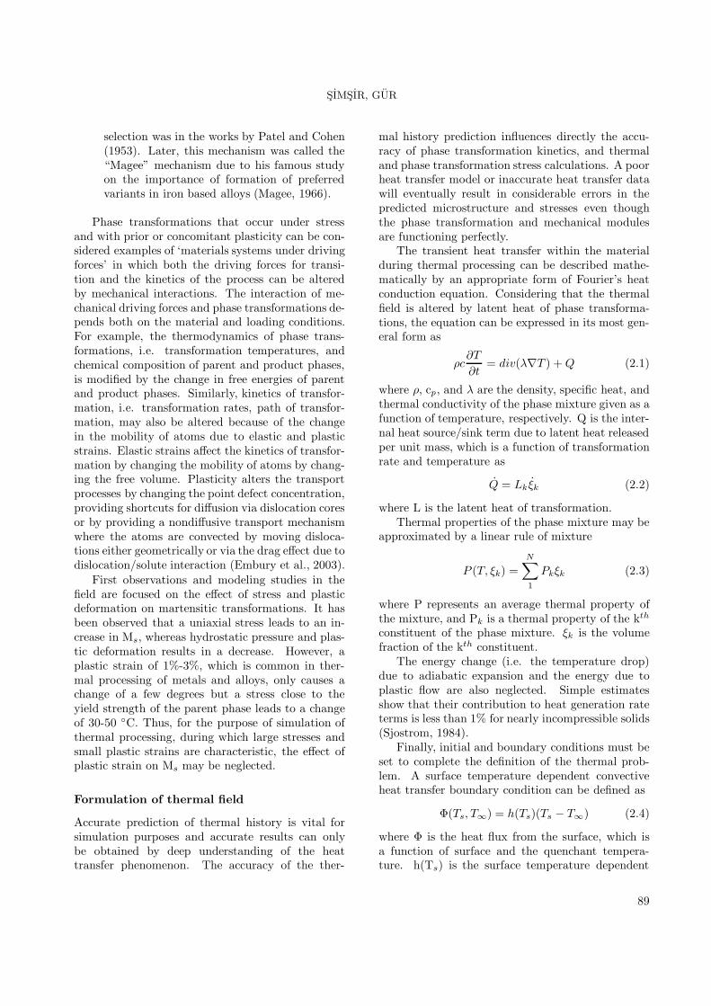
Figure 7 illustrates the comparison of XRD tangen-tial residual stress measurements with the ones pre-dicted by FE simulation. First of all, it can be seenthat the predicted surface residual stresses are ingood agreement with the experimental ones. An-other observation that can be made is that all of thespecimens except S1 have tensile type of tangentialstresses on the surface. The tangential stress stateon the surface is highly dependent on the hole di-ameter and has an increasing trend with increasinghole diameters. The critical hole diameter, at whichthe transition from compression to tension occurs, isa function of the hardenability of the steel and thequenching conditions.

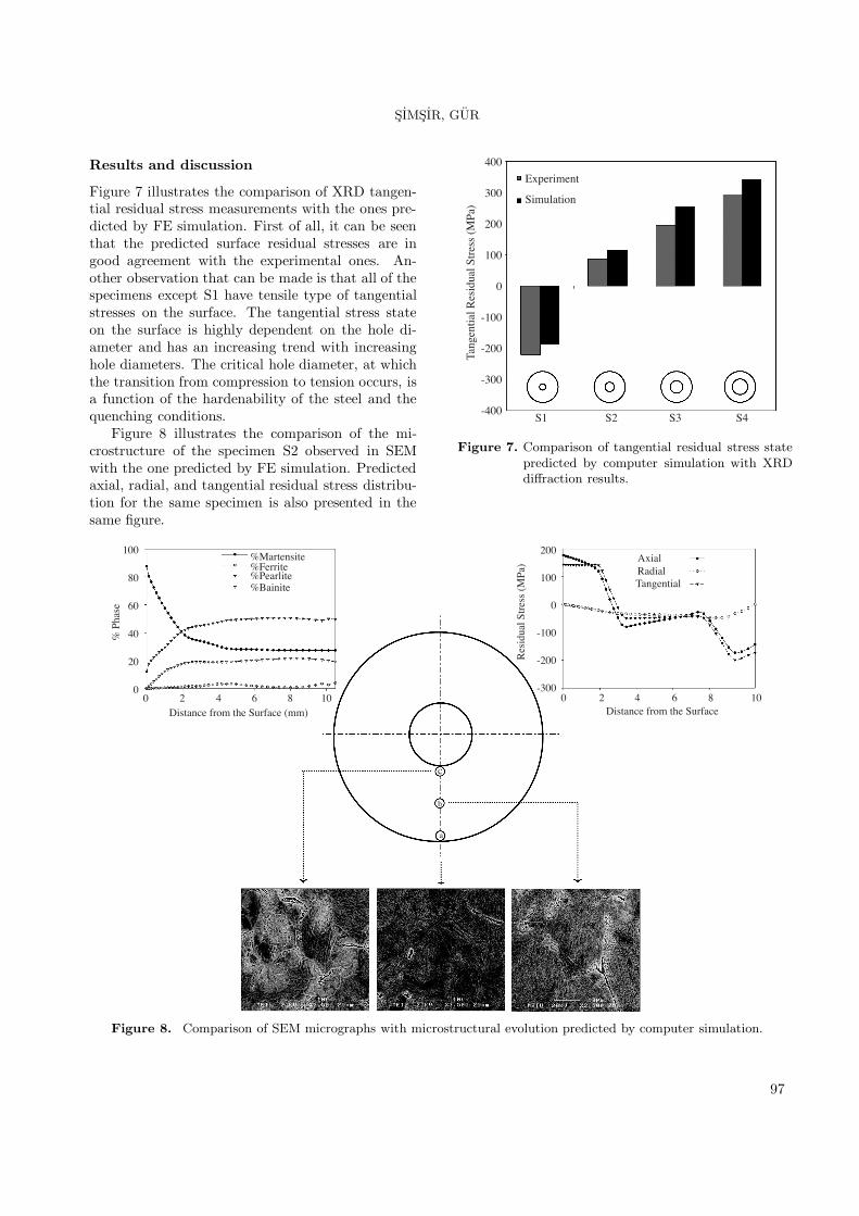
Figure 8 illustrates the comparison of the mi-crostructure of the specimen S2 observed in SEMwith the one predicted by FE simulation. Predictedaxial, radial, and tangential residual stress distribu-tion for the same specimen is also presented in thesame figure.

Experiment

Simulation

400

300

200

100

0

-100

-200

-300

-400

Tang

entia

l Res

idua

l Str

ess

(MPa

)

S1 S2 S3 S4

Figure 7. Comparison of tangential residual stress statepredicted by computer simulation with XRDdiffraction results.

200

100

0

-100

-200

-300

% P

hase

0 2 4 6 8 10Distance from the Surface (mm)

%Martensite%Ferrite%Pearlite%Bainite

AxialRadialTangential

0 2 4 6 8 10Distance from the Surface

100

80

60

40

20

0

Res

idua

l Str

ess

(MPa

)

c

b

a

Figure 8. Comparison of SEM micrographs with microstructural evolution predicted by computer simulation.

97

SIMSIR, GUR

From the micrograph it can be observed thatthe outer surface (a) consists of mostly marten-site, little bainite/pearlite, and trace amount of fer-rite. Simulation results reports 85% martensite, 10%pearlite, and 5% bainite for the same region. Sim-ilarly, the mid section (b) is made up of mostlypearlite/martensite mixture, some bainite, and asmall amount of ferrite. A composition of 50%pearlite, 33% martensite, 10% bainite, and 2% ferriteis predicted for the same region by computer simu-lation. Finally, the inner surface (c) has a pearliticmicrostructure with some martensite/bainite and anincreased amount of ferrite, whereas computer sim-ulation results indicate nearly 55% pearlite, 27%martensite, 14% bainite, and 4% ferrite. All of theseresults indicate a good match between the calculatedand observed microstructures.

Conclusion

Modeling is one of the most crucial elements in thedesign and optimization of thermal materials pro-cessing systems since it provides considerable ver-satility in obtaining quantitative results, which areneeded as inputs for an optimum design cycle. Inthis study, a mathematical framework capable ofpredicting temperature history, evolution of phases,and internal stresses during the thermal processingof materials was established. The model was inte-grated into commercial FEA software Msc.Marc byuser subroutines. The accuracy of the model wasverified by simulating the quenching of hollow steelcylinders. Simulation results were compared withSEM observations and XRD residual stress measure-ments. According to the results, it can be concludedthat

• The model can effectively predict the trendsin the distribution of the microstructure andresidual stresses. The accuracy of prediction isalso remarkable.

• The model has a modular design that allowssimulation of many thermal material process-ing techniques with minor revisions.

• Determination of final properties of the prod-uct after thermal material processing is an in-volving and challenging task. For example,even the effect of minor geometrical modifi-cations results in large variations in the mi-crostructure and residual stress distribution,

which cannot be expressed by a simple rule ofthumb.

Nomenclature

Indices

eq equilibrium valuemax maximum valueo represents an initial valuek property related to kth microstructural con-

stituent, any property without subscript kstands for the overall property of the phasemixture.

Operators

. scalar product

. time derivative

.. second time derivativeΔ increment operator∇ gradient operatordiv divergence operator

Vectors and Tensors

αij kinematic hardening (backstress) tensorδij Kronecker’s deltaεij total strain tensorεij total strain rate tensorεeij elastic strain rate tensor

εpij plastic strain rate tensor

εthij thermal strain rate tensor

εptij phase transformation dilatational strain rate

tensorεtpij transformation plasticity (TRIP) rate tensor

σij Cauchy stress tensorSij stress deviator

Matrices and Vectors

[B] matrix of spatial derivatives of shape func-tions

[C] conductivity matrix[D] damping matrix[H] heat capacity matrix[K] stiffness matrix[M] mass matrix{F} force vector

98

SIMSIR, GUR

{Q} nodal heat flux vector{QI} nodal heat flux vector due to deformation{QF } nodal heat flux vector due to friction{T} nodal temperature vector{

T}

nodal cooling rate vector{u} nodal displacement vector{u} nodal velocity vector{u} nodal acceleration vector

Latin Letters

b time coefficient for JMAK equationc specific heat capacityc∗ fictitious (modified) specific heatdλ plastic multiplierh convective heat transfer coefficientkB Stephan-Boltzmann constantn time exponent for JMAK equationr saturation parametert timeC kinematic hardening modulusE elastic modulusH plastic hardening modulusJ2 second invariant of stress deviatorK TRIP constantL latent heat of transformationMs martensite start temperature

N number of microstructural constituentsQtr internal heat source/sink termS Scheil’s sumT temperatureTs surface temperatureT∞ ambient temperature

Greek Letters

α linear thermal expansion coefficientεp equivalent plastic strainκ hardening parameterλ thermal conductivityν Poisson’s ratioρ densityσo yield strengthσf flow stressσm mean stressτ fictitious isothermal timeτs transformation start timeζ emissivityξ fraction of a microstructural constituentΔ structural dilatation due to phase transforma-

tionΦ heat fluxΩ Koistinen-Marburger constantΨ yield functional

References

Avrami, M., “Kinetics of Phase Change. I. General The-ory”, J. Chem. Phys., 7, 1103-1112, 1939.

Cahn, J.W., “Transformation Kinetics During Contin-uous Cooling”, Acta Metallurgica, 4, 572-575, 1956.

Cherkaoui, M., “Transformation Induced Plasticity:Mechanisms and Modeling”, Journal of EngineeringMaterials and Technology-Transactions of the ASME,124, 55-61, 2002.

Christian, J.W., The Theory of Transformations inMetals and Alloys, Pergamon Press, Oxford, 1975.

Colonna, F., Massoni, E., Denis, S., Chenot, J.L., Wen-denbaum, J. and Gauthier, E., “On Thermo-Elastic-Viscoplastic Analysis of Cooling Processes IncludingPhases Changes”, Journal of Materials Processing Tech-nology, 34, 525-532, 1992.

Denis, S., Boufoussi, M., Chevrier, J.C. and Simon, A.,“Analysis of the Development of Residual Stresses forSurface Hardening of Steels by Numerical Simulation:Effect of Process Parameters.”, International Confer-ence on Residual Stresses (ICRS4), 513-519, 1994.

Denis, S., Farias, D. and Simon, A., “Mathematical-Model Coupling Phase-Transformations and Tempera-ture Evolutions in Steels”, ISIJ International, 32, 316-325, 1992.

Denis, S., Gautier, E., Sjostrom, S. and Simon, A., “In-fluence of Stresses on the Kinetics of Pearlitic Transfor-mation during Continuous Cooling”, Acta Metallurgica,35, 1621-1632, 1987.

Embury, J.D., Deschamps, A. and Brechet, Y., “TheInteraction of Plasticity and Diffusion Controlled Pre-cipitation Reactions”, Scripta Materialia, 49, 927-932,2003.

Greenwood, G.W. and Johnson, R.H., “The Deforma-tion of Metals under Small Stresses during Phase Trans-formations”, Proc. Roy. Soc., 283, 403-422, 1965.

Gur, C.H. and Tekkaya, A.E., “Numerical Investigationof Non-Homogeneous Plastic Deformation in Quench-ing Process”, Materials Science and Engineering A, 319,164-169, 2001.

99

SIMSIR, GUR

Hsu, T.Y., “Additivity Hypothesis and Effects of Stresson Phase Transformations in Steel”, Current Opinionin Solid State & Materials Science, 9, 256-268, 2005.

Inoue, T. and Wang, Z.G., “Finite Element Analysis ofCoupled Thermoinelastic Problem with Phase Transfor-mation”, Int. Conf. Num. Meth. in Industrial FormingProcesses, 1982.

Inoue, T. and Wang, Z.G., “Coupling between Stress,Temperature, and Metallic Structures During ProcessesInvolving Phase-Transformations”, Materials Scienceand Technology, 1, 845-850, 1985.

Jaluria, Y., “Thermal Processing of Materials: FromBasic Research to Engineering”, Journal of HeatTransfer-Transactions of the ASME, 125, 957-979, 2003.

Koistinen, D.P. and Marburger, R.E., “A GeneralEquation Prescribing the Extent of the Austenite-Martensite Transformation in Pure Iron-Carbon Alloysand Plain Carbon Steels”, Acta Metallurgica, 7, 59-60,1959.

Loshkarev, V.E., “Mathematical Modeling of the Hard-ening Process with Allowance for the Effect of Stresseson Structural Transformations in Steel”, Metal Scienceand Heat Treatment, 28, 3-9, 1986.

Magee, C.L., “Transformation Kinetics, Micro-Plasticity and Ageing of Martensite in Fe-31ni”, PhD.Thesis, Carnegie Inst. of Tech., Pittsburgh , USA,1966.

Patel, J.R. and Cohen, M., “Criterion for the Actionof Applied Stress in the Martensitic Transformation”,Acta Metallurgica, 1, 531-538, 1953.

Rammerstorfer, F.G., Fischer, D.F., Mitter, W., Bathe,K.J. and Snyder, M.D., “On Thermo-Elastic-PlasticAnalysis of Heat-Treatment Processes Including Creepand Phase Changes”, Computers and Structures, 13,771-779, 1981.

Rammerstorfer, F.G., Fischer, F.D., Till, E. ., Mitter,W. and Grundler, O., The Influence of Creep and Trans-formation Plasticity in the Analysis of Stresses Due toHeat Treatment. Numerical Methods in Heat Transfer,447-460, 1983.

Scheil, E., “Anlaufzeit Der Austenitumwandlung”,Arch. Eisenhuttenwes, 8, 565-567, 1935.

Sjostrom, S., “Calculation of Quench Stresses in Steel”,PhD Thesis, University of Linkoping, Linkoping, Swe-den, 1982.

Sjostrom, S., “Interactions and Constitutive Models forCalculating Quench Stresses in Steel”, Materials Sci-ence and Technology, 1, 823-829, 1984.

Todinov, M.T., “Mechanism for Formation of the Resid-ual Stresses from Quenching”, Modelling and Simula-tion in Materials Science and Engineering, 6, 273-291,1998.

Zandona, M., Mey, A., Boufoussi, M., Denis, S. and Si-mon, A., Calculation of Internal Stresses during SurfaceHeat Treatment of Steels. Residual Stresses, 1011-1020,1993.

100