A Markov-Switching Multi-FractalInter-Trade Duration Model,

with Application to U.S. Equities

Fei Chen (HUST)Francis X. Diebold (UPenn)Frank Schorfheide (UPenn)

December 14, 20121 / 39

“Big Data”

Are big data informative for trends? No

Are big data informative for volatilities? Yes: realized volatility.

For durations? Yes: both trivially and subtly.

– Trivially: trade-by-trade data needed for inter-trade durations

– Subtly: time deformation links volatilities to durations.So big data inform us about vols which inform us about durations.

2 / 39

Why More Focus on Durations Now?

I We need better understanding of information arrival, tradearrival, liquidity, volume, market participant interactions, linksto volatility, etc.

I Financial market roots of the Great RecessionI Purely financial-market events like the Flash Crash

I The duration point process is the ultimate process of interest.It determines everything else, yet it remains incompletelyunderstood.

I Long memory is clearly present in calendar-time volatility andis presumably inherited from conditional intensity of arrivals intransactions time, yet there is little long-memory durationliterature.

3 / 39

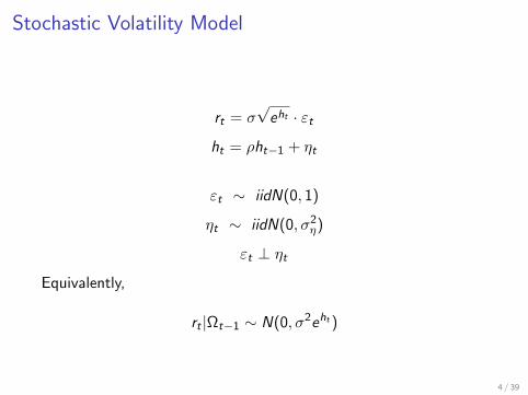
Stochastic Volatility Model

rt = σ√eht · εt

ht = ρht−1 + ηt

εt ∼ iidN(0, 1)

ηt ∼ iidN(0, σ2η)

εt ⊥ ηtEquivalently,

rt |Ωt−1 ∼ N(0, σ2eht )

4 / 39

From Where Does Stochastic Volatility Come?

Time-deformation modelof calendar time (e.g., “daily”) returns:

rt =eht∑i=1

ri

ht = ρht−1 + ηt

(trade-by-trade returns ri ∼ iidN(0, σ2), daily volume eht )

=⇒ rt |Ωt−1 ∼ N(0, σ2eht )

– Volume/duration dynamics produce volatility dynamics– Volatility properties inherited from duration properties

5 / 39

What Are the Key Properties of Volatility?

In general:

I Volatility dynamics fatten unconditional distributional tailse.g., rt |Ωt−1 ∼ N(0, σ2eht ) =⇒ rt ∼ “fat-tailed”

I Volatility dynamics are persistent

I Volatility dynamics are long memory

Elegant modeling framework that captures all properties:

Calvet and Fischer (2008),Multifractal Volatility:Theory, Forecasting, and Pricing,

Elsevier

6 / 39

Roadmap

I Empirical regularities in durations

I The MSMD model

I Preliminary empirics

7 / 39

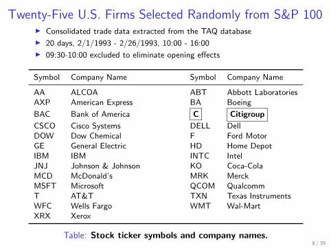
Twenty-Five U.S. Firms Selected Randomly from S&P 100I Consolidated trade data extracted from the TAQ database

I 20 days, 2/1/1993 - 2/26/1993, 10:00 - 16:00

I 09:30-10:00 excluded to eliminate opening effects

Symbol Company Name Symbol Company Name

AA ALCOA ABT Abbott LaboratoriesAXP American Express BA Boeing

BAC Bank of America C Citigroup

CSCO Cisco Systems DELL DellDOW Dow Chemical F Ford MotorGE General Electric HD Home DepotIBM IBM INTC IntelJNJ Johnson & Johnson KO Coca-ColaMCD McDonald’s MRK MerckMSFT Microsoft QCOM QualcommT AT&T TXN Texas InstrumentsWFC Wells Fargo WMT Wal-MartXRX Xerox

Table: Stock ticker symbols and company names.8 / 39

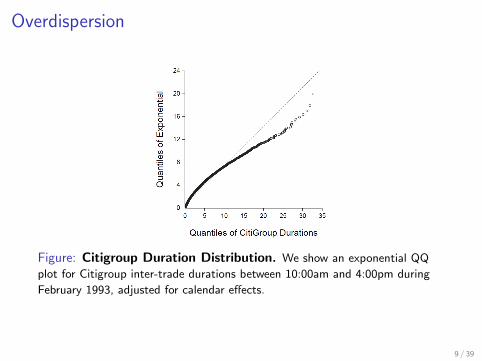
Overdispersion

Figure: Citigroup Duration Distribution. We show an exponential QQ

plot for Citigroup inter-trade durations between 10:00am and 4:00pm during

February 1993, adjusted for calendar effects.

9 / 39

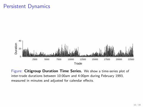
Persistent Dynamics

0

20

40

2500 5000 7500 10000 12500 15000 17500 20000 22500

Trade

Dur

atio

n

Figure: Citigroup Duration Time Series. We show a time-series plot of

inter-trade durations between 10:00am and 4:00pm during February 1993,

measured in minutes and adjusted for calendar effects.

10 / 39

Long Memory

.0

.1

.2

.3

25 50 75 100 125 150 175 200

Displacement (Trades)

Aut

ocor

rela

tion

Figure: Citigroup Duration Autocorrelations. We show the sample

autocorrelation function of Citigroup inter-trade durations between 10:00am

and 4:00pm during February 1993, adjusted for calendar effects.

11 / 39

Roadmap

I Empirical regularities in inter-trade durations!

I The MSMD model

I Empirics

12 / 39

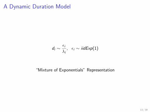
A Dynamic Duration Model

di ∼εiλi, εi ∼ iidExp(1)

“Mixture of Exponentials” Representation

13 / 39

Point Process Foundations

Ti (ω) > 0i∈1,2,... on (Ω,F ,P) s.t. 0 < T1(ω) < T2(ω) < · · ·

N(t, ω) =∑i≥1

1(Ti (ω) ≤ t)

λ(t) = lim∆t↓0

(1

∆tP[N(t + ∆t)− N(t) = 1 | Ft−]

)P(t1, . . . , tn|λ(·)) =

n∏i=1

(λ(ti ) exp

[−∫ ti

ti−1

λ(t)dt

])

If λ(t) = λi on [ti−1, ti ), then:

P(t1, . . . , tn|λ(·)) =n∏

i=1

(λi exp [−λidi ])

di ∼εiλi, εi ∼ iidExp(1)

How to parameterize the conditional intensity λi?14 / 39

Markov Switching Multifractal Durations (MSMD)

λi = λ

k∏k=1

Mk,i

λ > 0, Mk,i > 0, ∀k

Independent intensity components Mk,i

are Markov renewal processes:

Mk,i =

draw from f (M) w.p. γkMk,i−1 w.p. 1− γk

f (M) is identical ∀ k , with M > 0 and E (M) = 1

15 / 39

Modeling Choices

Simple binomial renewal distribution f (M):

M =

m0 w.p. 1/22−m0 w.p. 1/2,

where m0 ∈ (0, 2]

Simple renewal probability γk :

γk = 1− (1− γk)bk−k

γk ∈ (0, 1) and b ∈ (1,∞)

16 / 39

Renewal Probabilities

k

Ren

ewal

Pro

babi

lity,

γk

3 4 5 6 7

0.00

0.05

0.10

0.15

0.20

Figure: MSMD Intensity Component Renewal Probabilities. We

show the renewal probabilities (γk = 1 − (1 − γk)bk−k

) associated with the

latent intensity components (Mk), k = 3, ..., 7. We calibrate the MSMD model

with k = 7, and with remaining parameters that match our

subsequently-reported estimates for Citigroup.

17 / 39

All Together Now

di =εiλi

λi = λ

k∏k=1

Mk,i

Mk,i =

M w.p. 1− (1− γk)b

k−k

Mk,i−1 w.p. (1− γk)bk−k

M =

m0 w.p. 1/22−m0 w.p. 1/2

εi ∼ iid exp(1), k ∈ N, λ > 0, γk ∈ (0, 1), b ∈ (1,∞), m0 ∈ (0, 2]

parameters θk = (λ, γk , b,m0)′

k-dimensional state vector Mi = (M1,i ,M2,i , . . .Mk,i )

2k states18 / 39

MSMD Overdispersion

Figure: QQ Plot, Simulated Durations. N = 22, 988; parameters

calibrated to match Citigroup estimates.

19 / 39

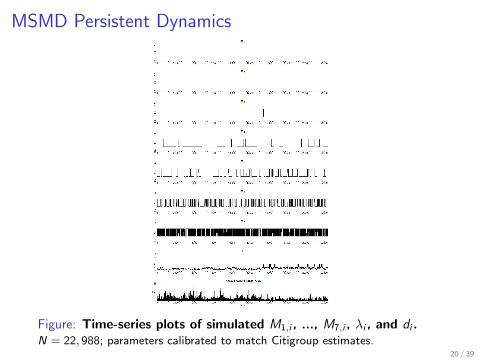
MSMD Persistent Dynamics

Figure: Time-series plots of simulated M1,i , ..., M7,i , λi , and di .N = 22, 988; parameters calibrated to match Citigroup estimates.

20 / 39

MSMD Long Memory

Displacement (Trades)

Aut

ocor

rela

tion

0 25 50 75 100 125 150 175 200

0.0

0.1

0.2

0.3

Figure: Sample Autocorrelation Function, Simulated Durations.N = 22, 988; parameters calibrated to match Citigroup estimates.

21 / 39

MSMD Long Memory

The MSMD autocorrelation function satisfies

supτ∈Ik

∣∣∣∣ ln ρ(τ)

ln τ−δ− 1

∣∣∣∣→ 0 as k →∞

δ = logb E (M2)− logb[E (M)]2

M =

2m−1

0

m−10 +(2−m0)−1

w.p. 12

2(2−m0)−1

m−10 +(2−m0)−1

w.p. 12

22 / 39

Literature I:Mean Duration vs. Mean Intensity

Mean Duration:

di = ϕiεi , εi ∼ iid(1, σ2)

– ACD: Engle and Russell (1998), ...– MEM: Engle (2002), ...

Mean Intensity:

di ∼εiλi, εi ∼ iidExp(1)

– MSMD– Bauwens and Hautsch (2006)

– Bowsher (2006)

23 / 39

Literature II:Observation- vs. Parameter-Driven Models

Observation-Driven:

Ωt−1 observed (like GARCH)

– ACD– MEM as typically implemented

– GAS

Parameter-Driven:

Ωt−1 latent (like SV)

– MSMD– SCD: Bauwens and Veredas (2004)

24 / 39

Literature III:Short Memory vs. Long Memory

Short Memory:

Quick (exponential) duration autocorrelation decay

– ACD as typically implemented– MEM as typically implemented

Long-Memory:

Slow (hyperbolic) duration autocorrelation decay

– MSMD– FI-ACD: Jasiak (1999)

– FI-SCD: Deo, Hsieh and Hurvich (2010)

25 / 39

Literature IV:Reduced-Form vs. Structural Long Memory

Reduced Form:

(1− L)dyt = vt , vt ∼ short memory

– FI-ACD– FI-SCD

Structural:

yt = v1t + ...+ vNt , vit ∼ short memory

– MSMD

26 / 39

Roadmap

I Empirical regularities in inter-trade durations!

I The MSMD model!

I Empirics

27 / 39

Twenty-Five U.S. Firms Selected Randomly from S&P 100I Consolidated trade data extracted from the TAQ database

I 20 days, 2/1/1993 - 2/26/1993, 10:00 - 16:00

I 09:30-10:00 excluded to eliminate opening effects

Symbol Company Name Symbol Company Name

AA ALCOA ABT Abbott LaboratoriesAXP American Express BA BoeingBAC Bank of America C CitigroupCSCO Cisco Systems DELL DellDOW Dow Chemical F Ford MotorGE General Electric HD Home DepotIBM IBM INTC IntelJNJ Johnson & Johnson KO Coca-ColaMCD McDonald’s MRK MerckMSFT Microsoft QCOM QualcommT AT&T TXN Texas InstrumentsWFC Wells Fargo WMT Wal-MartXRX Xerox

Table: Stock ticker symbols and company names.28 / 39

Coefficient of Variation

Cou

nt

1.0 1.2 1.4 1.6 1.8 2.0 2.2

02

46

8

Figure: Distribution of Duration Coefficients of Variation AcrossFirms. We show a histogram of coefficients of variation (the standard

deviation relative to the mean), as a measure of overdispersion relative to the

exponential. For reference we indicate Citigroup.

29 / 39

Displacement (Trades)

Aut

ocor

rela

tion

0 25 50 75 100 125 150 175 200

0.0

0.1

0.2

0.3

0.4

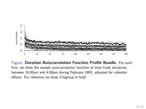
Figure: Duration Autocorrelation Function Profile Bundle. For each

firm, we show the sample autocorrelation function of inter-trade durations

between 10:00am and 4:00pm during February 1993, adjusted for calendar

effects. For reference we show Citigroup in bold.

30 / 39

MSMD Likelihood Evaluation (Using k = 2 for Illustration)

Each Mk , k = 1, 2 is a two-state Markov switching process:

P(γk) =

[1− γk/2 γk/2γk/2 1− γk/2

]Hence λi is a four-state Markov-switching process:

λi ∈ λs1s1, λs1s2, λs2s1, λs2s2

Pλ = P(γ1)⊗ P(γ2) (by independence of the Mk,i )

Likelihood function:

p(d1:n|θk) = p(d1|θk)n∏

i=2

p(di |d1:i−1, θk)

Conditional on λi , the duration di is Exp(λi ):

p(di |λi ) = λie−λidi

Weight by state probabilities obtained by the Hamilton filter.

31 / 39

k

Log−

Like

lihoo

d D

iffer

entia

l

3 4 5 6 7

−10

0−

80−

60−

40−

200

20

Figure: Maximized Log Likelihood Profile Bundle. We show likelihood

profiles for all firms as a function of k, in deviations from the value for k = 7,

which is therefore identically equal to 0. For reference we show Citigroup in

bold.

32 / 39

m0

Cou

nt

1.2 1.3 1.4 1.5

02

46

810

12

b

Cou

nt0 5 10 15 20 25 30

02

46

810

12λ

Cou

nt

1 2 3 4

02

46

810

γk

Cou

nt

0.0 0.2 0.4 0.6 0.8 1.0

02

46

810

1214

Figure: Distributions of MSMD Parameter Estimates Across Firms,k = 7. We show histograms of maximum likelihood parameter estimates

across firms, obtained using k = 7. For reference we indicate Citigroup.

33 / 39

k

Ren

ewal

Pro

babi

lity,

γk

3 4 5 6 7

0.0

0.2

0.4

0.6

0.8

1.0

Figure: Estimated Intensity Component Renewal Probability ProfileBundle, k = 7. For reference we show Citigroup in bold.

34 / 39

0.0

0.2

0.4

0.6

0.8

1.0

0.0 0.2 0.4 0.6 0.8 1.0

CD

F

P-Value

Citi

Figure: Empirical CDF of White Statistic p-Value, k = 7. For

reference we indicate Citigroup.

35 / 39

D = BICMSMD − BICACD

Cou

nt

0 100 200 300 400 500 600

02

46

8

Figure: Distribution of Differences in BIC Values Across Firms. We

use −BIC/2 = ln L− k ln(n)/2, and we compute differences as MSMD(7) -

ACD(1,1). We show a histogram. For reference we indicate Citigroup.

36 / 39

1−Step RMSE Difference

Cou

nt

−1.0 −0.5 0.0

05

1015

5−Step RMSE DifferenceC

ount

−4.5 −4.0 −3.5 −3.0 −2.5 −2.0 −1.5 −1.0

02

46

810

1220−Step RMSE Difference

Cou

nt

−4 −3 −2 −1 0

02

46

8

Figure: Distribution of Differences in Forecast RMSE Across Firms.We compute differences MSMD(7) - ACD(1,1). For reference we indicate

Citigroup.

37 / 39

Roadmap

I Empirical regularities in inter-trade durations!

I The MSMD model!

I Empirics!

38 / 39

Future Directions

I Additional model assessment

I Current data (using ultra-accurate time stamps)

I Panel of trading months.

Structural change?

39 / 39