a markov method for ranking college football conferences - math
TRANSCRIPT
A Markov Method for Ranking
College Football Conferences
R. Bruce Mattingly and Amber J. MurphySUNY Cortland
1 Introduction
The use of mathematical methods to develop rankings of sports teams iscertainly not a new idea. See for instance, Ford [7]. Ranking methods areparticularly important in Division I college football, because unlike nearlyany other sport, the champion is not determined through a playoff system.Instead, the Bowl Championship Series (BCS) Standings are used to selectthe two teams that will compete for the national championship. The BCSStandings are determined through a combination of two human polls andsix computer ranking methods [2]. These methods take a variety of factorsinto account, including a team’s individual win-loss record, its strength ofschedule, and so on. Most college teams are affiliated with conferences, andthe reputations of the various conferences can have a large influence on theteam rankings, particularly in the human polls. Jeff Sagarin’s NCAA footballratings published in USA Today [20] include conference rankings as well asrankings of individual teams. There is a great deal of interest in rankingmethods for college football. Kenneth Massey maintains an extensive web site[14] that provides information on an astonishing number of ranking methodsin addition to his own. For instance, in the 2008 season, Massey comparedthe rankings produced by 113 different methods [13].
A natural approach to developing a mathematical ranking method is tocreate a matrix whose entries are determined in some way by the results ofgames played between teams. Keener [8] discussed a method in which theranking of teams is derived from the computation of the dominant eigenvectorof a non-negative matrix. Massey [10] took an approach that involves thesolution of a least squares problem. Colley [4] developed a method that alsoinvolves the solution of a linear system of equations. The Massey and Colleymethods are both used by the BCS, as is Sagarin’s method. Matrix methodsbased on Markov Chains have been proposed by Redmond [17] and Govanet al. [5]. The latter method is a generalization of the Google PageRankalgorithm developed by Page et al. [16].
1
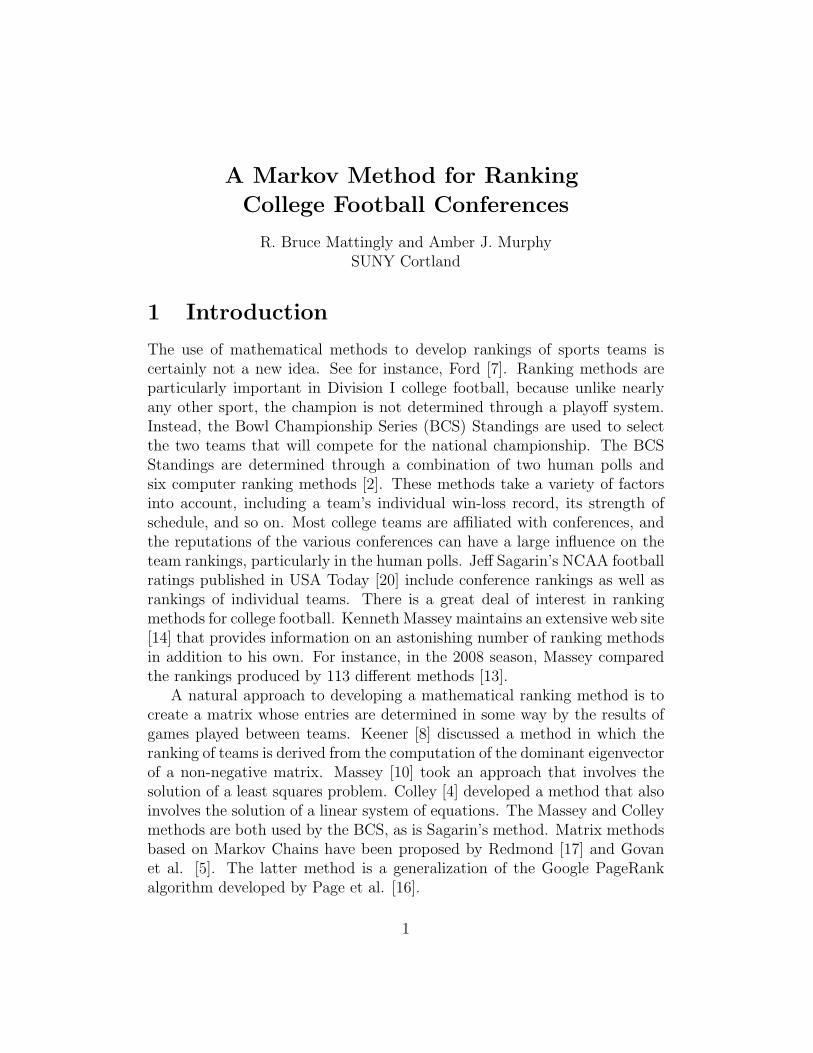
In this paper we propose a Markov method that is also similar to thePageRank idea. Our method takes advantage of the block structure that isparticularly evident in college football due to the low number of games played(relative to other sports such as basketball) and the fact that most teams areaffiliated with conferences. For the most part, teams within conferences allplay each other (some larger conferences are further divided into two divi-sions), and there are comparatively fewer interconference games. Because ofthis, a matrix whose entries are determined by the outcomes of games canbe partitioned very nicely into a block structure in which the dense diag-onal blocks represent conference games, and the sparse off-diagonal blockscorrespond to inter-conference matchups. Figure 1 shows the structure ofthe adjacency matrix that corresponds to the 2006 Division I college footballseason, where each nonzero entry represents a game between two teams.
Figure 1: Adjacency Matrix for 2006 Season
To exploit this natural block structure, we propose the use of the methodof stochastic complementation developed by Meyer [15]. This method pro-
2

vides a natural way to subdivide the original Markov chain into severalsmaller chains, each of which would represent a single conference. The sta-tionary distribution vector (or steady state vector) of each smaller chain canbe computed independently. These vectors can then be combined to producethe stationary distribution vector of the original Markov chain. This processinvolves the computation of a coupling matrix that represents yet anotherMarkov chain in which all of the teams in a particular conference are ag-gregated into a single state. A benefit of this approach is that, in additionto ranking the individual teams, the stationary distribution vector of thecoupling matrix provides a natural way to rank the conferences.
2 Overview of the method
The basic idea of our Markov chain approach to team ranking is straight-forward. Each state in the Markov chain corresponds to one football team,and transitions are only allowed between teams that have played each other.Our ranking method can be thought of as an iterative procedure that occursat the end of the season. Suppose that we have a large number of collegefootball fans who (as improbable as this sounds) have no preference for whichteam they support. Initially we distribute the fans equally among all avail-able teams. At each iteration of our method, a fan can choose to eitherremain with the same team or change to another team. The probability thata fan remains with a given team should be higher for a winning team than itis for a losing team. If a fan does not remain with the same team, it mightseem logical to assign the fan (with equal probability) to any of the teamsto whom the current team lost. Markov chain theory guarantees that if thetransition matrix is irreducible and aperiodic, then the iterative process willalways converge to a unique steady state vector [3, p. 222]. The percentageof fans assigned to each team would therefore represent that team’s rating.We sort the rating vector in decreasing order, and then each team’s positionin the sorted vector represents its ranking.
A potential problem with this approach is that if there are undefeatedteams, they would represent absorbing states in our Markov chain. In thecase where we had only one undefeated team, all of the fans would end upassigned to that single team. Our ranking vector would not be particularlyuseful, because the undefeated team would be ranked first, with everyoneelse tied for second. We therefore make the following adjustment: we allow
3

transitions between teams who played each other in both directions.The guiding principles that we used in developing our ranking method
are easy to describe qualitatively: the probability of a fan remaining witha team should be higher for a winning team than for a losing team, and ifa fan changes teams, transitions to teams that defeated the current teamshould occur with higher probability than transitions to teams who lost tothe current team. Determining the specific probabilities that should be usedbecame the central focus of our research.
Algorithm 1 describes our method for constructing the transition matrix.
Input: List of results of all games between a set of teamsOutput: A stochastic matrix with transition probabilities based on
game resultsLet N = maximum number of games played by any team;Let p = a value in the interval (0.5, 1.0);foreach Game k do
Let i = index of team that won game k;Let j = index of team that lost game k;aji = p;aij = 1− p;
endforeach Team i do
aii = N −∑j 6=i aij;
endA = A/N;
Algorithm 1: Construction of transition matrix
Algorithm 1 assumes that the same two teams never play more thanonce. In college football, exceptions to this can occur, particularly in largeconferences that have a conference championship game between the winnersof the two divisions after the regular season games, but before the bowlgames. Rematches could also occur in bowl games, but our interest was indetermining rankings before the bowl games began so that we could compareour results to the official BCS standings that were used to select the top twoteams. In both 2006 and 2008, one conference championship game was arematch, and in 2007 there were 3 rematches. We dealt with rematches inthe following way: if two teams played each other twice with the same winnereach time, we made no adjustment to our transition matrix. If the teams
4
split the two games, then we reasoned that transitions between the two teamsshould be equally likely in either direction, so we set aij = aji = 0.5 regardlessof the value of p that we were using.
3 Illustrative Examples
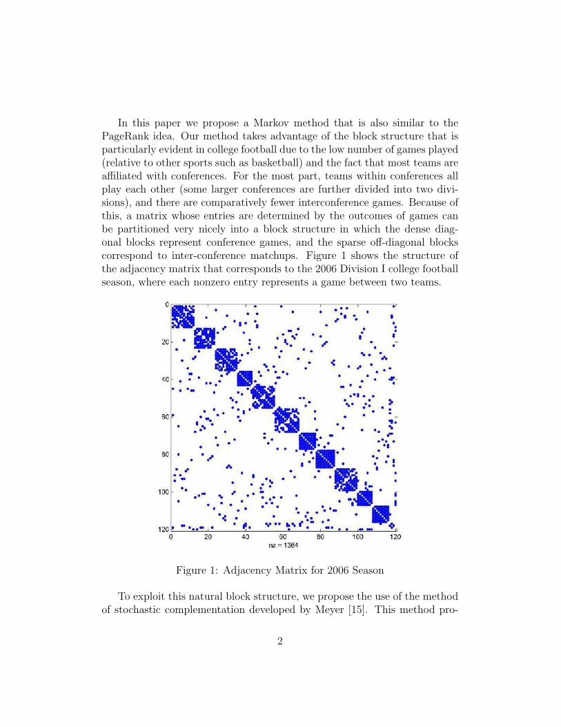
Example 1. Our first example demonstrates the construction of the transi-tion matrix. It involves only six teams, so we do not deal with partitioningthe Markov chain into smaller chains. We assume that each team plays only 3games, and the hypothetical results of these games are summarized in Table1.
Team Wins Losses1 4, 5, 6 none2 3 4, 53 4,6 24 2 1, 35 2, 6 16 none 1, 3, 5
Table 1: Game Results for Example 1
To construct the transition matrix, we follow the steps below. For pur-poses of this example we chose p = 0.8.
• Step 1: If i beats j, set aji = 0.8 and set aij = 0.2, producing thefollowing matrix:
0 0 0 0.2 0.2 0.20 0 0.2 0.8 0.8 00 0.8 0 0.2 0 0.2
0.8 0.2 0.8 0 0 00.8 0.2 0 0 0 0.20.8 0 0.8 0 0.8 0
• Step 2. In this step we adjust the diagonal entries so that all rowsums in the matrix are constant. While teams never play themselves,the diagonal entry represents the probability that a fan will stay with
5

the current team rather than changing to a new one. We accomplishthis as follows. For each row of the matrix, set aii = N − ∑
i 6=j aij,where N is the total number of games played by each team. In thisexample, N = 3. In the event that each team does not play the samenumber of games, this value just needs to be large enough to ensurethat the diagonal entry is non-negative. In our experiments on actualdata, we used N = 13 since teams normally play 12 regular seasongames, and a few teams also play a conference championship game.After this adjustment, all rows sums are the same. We then divide theentire matrix by N (3 in this example) to create a stochastic matrix.Our matrix now looks like this:
0.8000 0 0 0.0667 0.0667 0.06670 0.4000 0.0667 0.2667 0.2667 00 0.2667 0.6000 0.0667 0 0.0667
0.2667 0.0667 0.2667 0.4000 0 00.2667 0.0667 0 0 0.6000 0.06670.2667 0 0.2667 0 0.2667 0.2000
Note: In the methods described by Keener, if i defeats j, then aij is close
to 1, and aji is close to zero. Here, we have those two entries transposed.Since our method uses Markov chains, it bears some resemblance to themethods used for Google’s PageRank algorithm as described in Langvilleand Meyer [9, pp. 31–34]. In that work, aij is set to some nonzero valuewhenever there is a link from page i to page j. In other words, page i isrecommending page j as an “authority” by virtue of its link. The analogyhere is that team j “recommends” team i if j was defeated by i.
The steady state vector for this Markov chain is given below:
( 0.4515 0.0858 0.1240 0.1021 0.1741 0.0625 )
According to these values, the teams should be ranked in the followingorder: 1, 5, 3, 4, 2, 6. This is consistent with the teams’ win-loss records.Team 1 was undefeated and Team 6 was winless. Teams 5 and 3 both wontwo games, but Team 5 lost only to Team 1. Teams 4 and 2 each had onlyone win, but Team 4 defeated Team 2. Note that Team 2 actually defeateda higher-ranked team (Team 3). We adopt the terminology used by Ali etal. [1] and refer to this situation as a “violation.” It is virtually impossibleto develop a ranking system that avoids violations. Although we can define
6
a relation on a set of teams according to who defeated whom, such a relationis clearly not transitive. In this example, 3 beat 4, 4 beat 2, but 2 beat3. Next, we present a series of examples that demonstrate how the methodof stochastic complementation can be used to rank conferences, as well asteams.
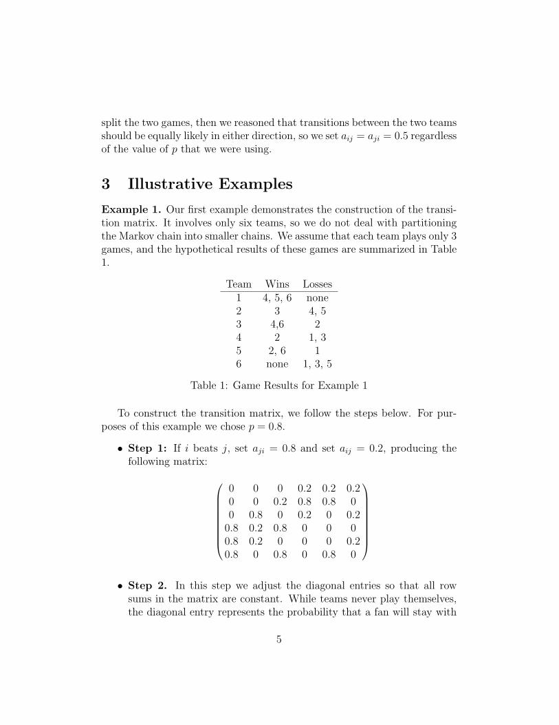
Example 2. We assume that we have 10 teams divided into two 5-member conferences. Each team plays every other team in their own confer-ence, but only one team from the other conference, for a total of 5 games.Our hypothetical results are given in Table 2.
West Conference Non-conference East Conference Non-conferenceWins Wins Wins Wins
1 2, 3, 4, 5 6 6 7, 8, 9, 10 none2 3, 4, 5 7 7 8, 9, 10 none3 4, 5 none 8 9, 10 34 5 9 9 10 none5 none 10 10 none none
Table 2: Game Results for Example 2
We deliberately constructed this example so that within each conference,there is a clear ordering (1 > 2 > 3 > 4 > 5) and (6 > 7 > 8 > 9 > 10)so that we can focus our attention on comparing the two conferences. UsingAlgorithm 1 with p = 0.80 we obtain the following transition matrix:
A =
0.80 0.04 0.04 0.04 0.04 0.04 0 0 0 00.16 0.68 0.04 0.04 0.04 0 0.04 0 0 00.16 0.16 0.44 0.04 0.04 0 0 0.16 0 00.16 0.16 0.16 0.44 0.04 0 0 0 0.04 00.16 0.16 0.16 0.16 0.32 0 0 0 0 0.040.16 0 0 0 0 0.68 0.04 0.04 0.04 0.04
0 0.16 0 0 0 0.16 0.56 0.04 0.04 0.040 0 0.04 0 0 0.16 0.16 0.56 0.04 0.040 0 0 0.16 0 0.16 0.16 0.16 0.32 0.040 0 0 0 0.16 0.16 0.16 0.16 0.16 0.20
To exploit the natural block structure induced by the conference schedul-
ing, we partition A as follows:
7

A =(A11 A12
A21 A22
)where each submatrix in this example is 5× 5. In general, only the diagonalblocks need to be square, with the size of each conforming to the size of thatparticular conference.
The stochastic complements are computed according to the formulas be-low (see Meyer for further details):
S11 = A11 + A12(I − A22)−1A21
S22 = A22 + A21(I − A11)−1A12
For this example, the matrices turn out to be:
S11 =
0.8279 0.0461 0.0412 0.0428 0.04210.1745 0.6994 0.0412 0.0428 0.04210.2327 0.2036 0.4594 0.0539 0.05040.1752 0.1691 0.1618 0.4518 0.04220.1752 0.1691 0.1618 0.1642 0.3298
and
S22 =
0.7533 0.0633 0.0867 0.0497 0.04690.2156 0.6011 0.0867 0.0497 0.04690.1711 0.1656 0.5800 0.0419 0.04140.2133 0.1867 0.2133 0.3400 0.04670.2133 0.1867 0.2133 0.1711 0.2156
For each stochastic complement, we can compute the unique station-
ary distribution vectors which satisfy v1S11 = v1, v1e = 1 and v2S22 =v2, v2e = 1, where e is a column vector of all 1’s. In this case, our resultsare as follows:
v1 = ( 0.5208 0.2310 0.1013 0.0866 0.0603 )
and
v2 = ( 0.4461 0.2175 0.2041 0.0772 0.0551 )
Note that in each vector, the entries appear in decreasing order, consistentwith the ordering that was determined by the results of the conference games.
8

Our primary interest here is in finding the coupling matrix C, whose entriesare given by cij = viAije. In our example, the coupling matrix is:
C =(
0.9478 0.05220.1355 0.8645
)and its stationary distribution vector is
w = ( 0.7221 0.2779 )
In this simple example, the Western conference has a higher rating (0.7221)than the Eastern conference (0.2779), which seems reasonable, given that inhead to head competition, Western conference teams won 4 of 5 games. Inthe next couple of examples, we will leave the conference results unchanged,but adjust the inter-conference results to see the effect upon the stationaryvector of the coupling matrix.
Example 3. In this example, the results of the conference games areunchanged, but this time, teams from the Western Conference win 3 of the5 inter-conference games as shown in Table 3.
West Conference Non-conference East Conference Non-conferenceWins Wins Wins Wins
1 2, 3, 4, 5 6 6 7, 8, 9, 10 none2 3, 4, 5 none 7 8, 9, 10 23 4, 5 8 8 9, 10 none4 5 none 9 10 45 none 10 10 none none
Table 3: Game Results for Example 3
In the interest of space we do not display the 10 × 10 stochastic matrixor the stochastic complements. Adjusting the off-diagonal blocks as notedabove leads to the following new coupling matrix:
C =(
0.9314 0.06860.1087 0.8913
)whose stationary distribution vector is given by
w = ( 0.6132 0.3868 )
9

Note that the Western conference still receives a higher rating than theEastern conference (0.6132 vs. 0.3868), but the difference is less pronouncedthan we saw in Example 2.
Example 4. In this final example, we again only change the inter-conference results as shown in Table 4.
West Conference Non-conference East Conference Non-conferenceWins Wins Wins Wins
1 2, 3, 4, 5 none 6 7, 8, 9, 10 12 3, 4, 5 none 7 8, 9, 10 23 4, 5 8 8 9, 10 none4 5 9 9 10 none5 none 10 10 none none
Table 4: Game Results for Example 4
Adjusting the off-diagonal blocks as noted above leads to the followingcoupling matrix:
C =(
0.8850 0.11500.0657 0.9343
)The new stationary distribution vector is given by
w = ( 0.3636 0.6364 )
Note that in this case, the Eastern conference receives the higher ratingand is therefore ranked first. Although they only won 2 of the 5 games, their2 wins came at the expense of the strongest teams in the Western conference.So this method gives more weight to 2 wins against strong teams, as opposedto 3 wins against weaker teams. We hesitate to over-analyze these examples,whose primary purpose is to illustrate how the method works. In the nextsection, we discuss our experiences in applying this method to actual data.
4 Experimental Results
We tested our ranking method using the complete game results for all 120college teams in the Division I Football Bowl Subdivision (FBS) from the2006, 2007 and 2008 seasons. (Note: in 2006, there were only 119 FBSteams, as Western Kentucky did not join this subdivision until 2007.)
10

Teams in the FBS occasionally play teams from lower divisions. We didnot have ready access to complete game data for the teams from the lowerdivisions, and made the decision to discard game results involving non-FBSteams. In most cases, the FBS teams won these games as expected, withsome notable exceptions. For instance, traditional power Michigan lost toAppalachian State in 2007. We recognize that in a few cases, teams who lostto non-FBS teams would benefit with a higher ranking than they would havereceived had we considered these results. However, we felt that discardingthese games would have a minimal effect on our results, since for the mostpart they affected only lower-ranked teams. Table 5 shows for each yearthe number of games played by FBS teams against non-FBS opponents, thenumber of losses to such teams, and the highest BCS rank of a team fromthe FBS that had such a loss.
Year Games Losses Rank2006 78 7 632007 80 9 292008 86 2 108
Table 5: Games involving non-FBS teams
Data for this study was obtained from an Internet site maintained byJames Howell [6]. We wrote C++ code to extract the information that weneeded from the raw data and to create the transition matrix. Matlab wasused for all of the matrix computations. The main focus of our effort was toexperiment with the values of the transition probabilities that we assignedfor wins and losses. In the examples above, we used p = 0.80. In ourexperiments, we tested values of p between 0.55 and 0.95 in increments of0.05. Note: a value of p = 0.50 would not be useful, because it would meanthat transitions between teams would occur in either direction with equallikelihood. The resulting steady state vector would therefore be the vector ofall ones (normalized by the number of teams.) In other words, all 120 teamswould be ranked equally.
Google’s PageRank algorithm inspired one other variation that we tested.In the PageRank algorithm, transitions between states (web pages) occurprimarily due to explicit links between pages. It is recognized, however, thatsurfers sometimes do not follow links, but have the ability to jump to anyother web page simply by typing in a new URL. We wanted to incorporatethis idea into our ranking method in accordance with the old adage that
11

“on any given day” any team is capable of defeating any other team. Toimplement this, transition matrix A is constructed according to Algorithm1. A second matrix G is created, with each entry equal to 1/N where N isthe number of teams. In matrix G, a transition from any team to any otherteam is equally likely. The final transition matrix is the weighted sum
αA+ (1− α)G.
Langville and Meyer [9, p. 41] report that in the case of ranking web pages,Google gets the best results using α = 0.85. In our tests, the values of α thatwe used ranged from 0.80 to 1.00 in increments of 0.05. For values of α < 1,we could use p = 1 in the construction of matrix A since the incorporationof the G matrix would prevent absorbing states.
Our rankings were based on the results of games played through the end ofthe regular season, including conference championships for those conferencesthat have them, but not the bowl games. We then counted the number ofviolations, that is, the number of regular season games in which a game waswon by a lower-ranked team. Our assumption is that, given a choice betweentwo ranking methods, the one that produces the lower number of violationsis preferred.
The graphs shown in Figures 2, 3 and 4 summarize the performance ofthe ranking methods that we tested on actual data from the 2006, 2007 and2008 seasons. The horizontal axis in each graph shows the values of p thatwe tested (before the rows of the matrix were normalized.) The verticalaxis shows the number of violations. Each graph includes 5 sets of data,corresponding to the values of α that we tested.
We make two observations about our results from these three seasons.First of all, the method generally produced fewer violations when lower valuesof p were used. In each of the three years, the fewest violations were producedusing either p = 0.55 or p = 0.60. Secondly, it appears that using the Gmatrix to allow transitions between all teams generally increased the numberof violations, although in 2006, the combination of p = 0.55 and α = 0.95produced the best results.
Table 6 compares the performance of our best method for each yearagainst the final BCS standings as reported on Massey’s web site at theend of the regular season but before the bowl games [11, 12, 13]. We reportthe number of violations in the rankings produced by each method. We werealso interested in how accurately each method could “predict” the winners
12

Figure 2: Test results from 2006 season
Figure 3: Test results from 2007 Season
13

Figure 4: Test results from 2008 Season
Year Method Number Violations Number Bowlof Games of Bowls Upsets
2006 p = 0.55, α = 0.95 682 107 32 11BCS 107 11
2007 p = 0.55, α = 1.0 686 132 32 10BCS 128 14
2008 p = 0.60, α = 1.0 683 120 34 17BCS 125 19
Table 6: Performance Comparison for Ranking Methods
of the bowl games that are played after the regular season games. If a teamwins a bowl game against a higher-ranked opponent, we refer to this as an“upset.” It might appear that an upset is just another name for a violation,but there is one difference – the results of the bowl games were not consideredwhen the rankings were calculated.
It appears that generally, our method produces comparable results tothe BCS rankings, but there is no clear pattern. Not surprisingly, bothmethods did a better job on the regular season games than on the bowlgames. The number of violations was consistently in the range of 16–19%.By contrast, the number of bowl upsets ranged from 31% to 56%. In 2006,the two methods had the same number of violations and failed to predict11 bowl games correctly (out of 32.) In 2007, our best method produced
14

more violations than the BCS rankings, but we had fewer bowl upsets. In2008, our best method produced fewer violations than the BCS rankings. Inthat year, neither method did a particularly good job of predicting the bowlgame results, although we did slightly better than the BCS, predicting 50%correctly (17 out of 34.)
We were also curious to compare the teams that would have been selectedto play in the BCS championship game based on our results. Tables 7, 8 and9 list the top 5 teams as ranked by our best method, and also shows howthose teams fared in the official BCS rankings published at the end of theregular season.
Team Our rank BCS rankFlorida 1 2Ohio State 2 1Southern California 3 4Michigan 4 3Louisville 5 6
Table 7: 2006 Team Rankings
Team Our rank BCS rankMissouri 1 6Virginia Tech 2 3Georgia 3 5Louisiana State 4 2Ohio State 5 1
Table 8: 2007 Team Rankings
Team Our rank BCS rankOklahoma 1 1Florida 2 2Texas 3 3Texas Tech 4 7Utah 5 6
Table 9: 2008 Team Rankings
15
In 2006, our method would have selected the same two teams (Floridaand Ohio State) for the BCS championship game, although we had the toptwo teams reversed, and as it turns out, Florida won the game. In 2008, thecorrelation was even stronger – our method agreed with the BCS rankings onthe top three teams. In 2007, the results were quite different. Our top twoteams (Missouri and Virginia Tech) were ranked 6th and 3rd, respectively,by the BCS. It is worth noting, however, that Missouri lost to Oklahoma intheir conference championship game. Prior to that loss, Missouri had beenranked first in the BCS. Missouri’s only other loss was also to Oklahoma,earlier in the season. In that light, the results of our ranking method aremore understandable – Missouri’s loss in the conference championship gameprovided no new information.
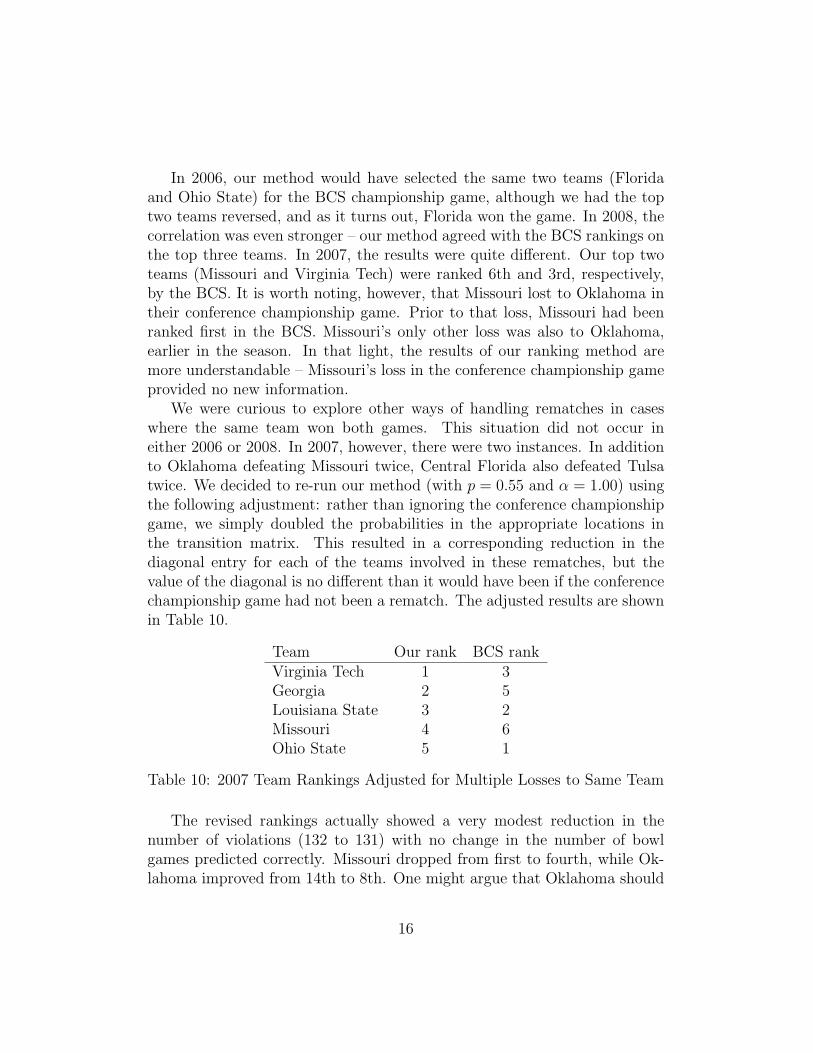
We were curious to explore other ways of handling rematches in caseswhere the same team won both games. This situation did not occur ineither 2006 or 2008. In 2007, however, there were two instances. In additionto Oklahoma defeating Missouri twice, Central Florida also defeated Tulsatwice. We decided to re-run our method (with p = 0.55 and α = 1.00) usingthe following adjustment: rather than ignoring the conference championshipgame, we simply doubled the probabilities in the appropriate locations inthe transition matrix. This resulted in a corresponding reduction in thediagonal entry for each of the teams involved in these rematches, but thevalue of the diagonal is no different than it would have been if the conferencechampionship game had not been a rematch. The adjusted results are shownin Table 10.
Team Our rank BCS rankVirginia Tech 1 3Georgia 2 5Louisiana State 3 2Missouri 4 6Ohio State 5 1
Table 10: 2007 Team Rankings Adjusted for Multiple Losses to Same Team
The revised rankings actually showed a very modest reduction in thenumber of violations (132 to 131) with no change in the number of bowlgames predicted correctly. Missouri dropped from first to fourth, while Ok-lahoma improved from 14th to 8th. One might argue that Oklahoma should
16
be ranked ahead of Missouri by virtue of their two wins, but it is worth con-sidering that Oklahoma lost two games in 2007 to Colorado and Texas Tech,and that Missouri defeated both of these teams.
The final variation that we considered was to construct the transitionmatrix using variable probabilities based on the final score of each game.Our method for computing transition probabilities is similar to an approachdescribed by Keener. Assuming that Team i loses to Team j by a score of sj
to si, the general formula is given by
pij =sj + A
si + sj + 2A
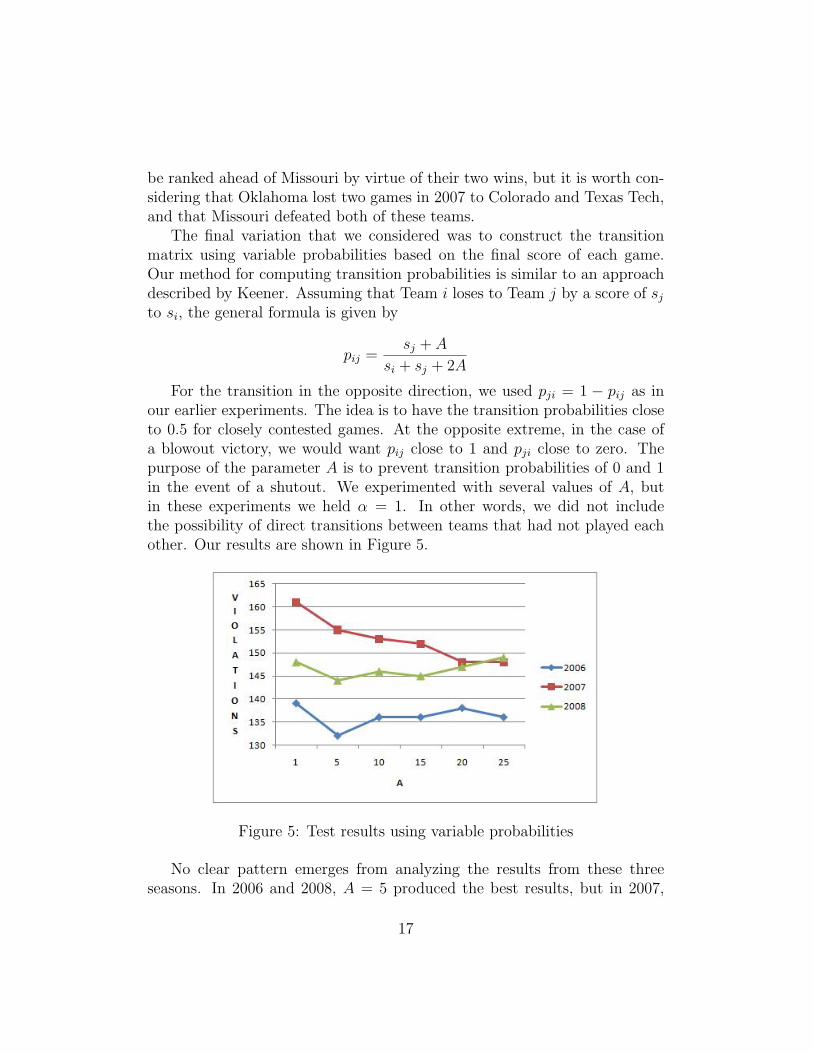
For the transition in the opposite direction, we used pji = 1 − pij as inour earlier experiments. The idea is to have the transition probabilities closeto 0.5 for closely contested games. At the opposite extreme, in the case ofa blowout victory, we would want pij close to 1 and pji close to zero. Thepurpose of the parameter A is to prevent transition probabilities of 0 and 1in the event of a shutout. We experimented with several values of A, butin these experiments we held α = 1. In other words, we did not includethe possibility of direct transitions between teams that had not played eachother. Our results are shown in Figure 5.
Figure 5: Test results using variable probabilities
No clear pattern emerges from analyzing the results from these threeseasons. In 2006 and 2008, A = 5 produced the best results, but in 2007,
17
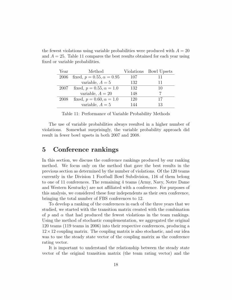
the fewest violations using variable probabilities were produced with A = 20and A = 25. Table 11 compares the best results obtained for each year usingfixed or variable probabilities.
Year Method Violations Bowl Upsets2006 fixed, p = 0.55, α = 0.95 107 11
variable, A = 5 132 112007 fixed, p = 0.55, α = 1.0 132 10
variable, A = 20 148 72008 fixed, p = 0.60, α = 1.0 120 17
variable, A = 5 144 13
Table 11: Performance of Variable Probability Methods
The use of variable probabilities always resulted in a higher number ofviolations. Somewhat surprisingly, the variable probability approach didresult in fewer bowl upsets in both 2007 and 2008.
5 Conference rankings
In this section, we discuss the conference rankings produced by our rankingmethod. We focus only on the method that gave the best results in theprevious section as determined by the number of violations. Of the 120 teamscurrently in the Division 1 Football Bowl Subdivision, 116 of them belongto one of 11 conferences. The remaining 4 teams (Army, Navy, Notre Dameand Western Kentucky) are not affiliated with a conference. For purposes ofthis analysis, we considered these four independents as their own conference,bringing the total number of FBS conferences to 12.
To develop a ranking of the conferences in each of the three years that westudied, we started with the transition matrix created with the combinationof p and α that had produced the fewest violations in the team rankings.Using the method of stochastic complementation, we aggregated the original120 teams (119 teams in 2006) into their respective conferences, producing a12×12 coupling matrix. The coupling matrix is also stochastic, and our ideawas to use the steady state vector of the coupling matrix as the conferencerating vector.
It is important to understand the relationship between the steady statevector of the original transition matrix (the team rating vector) and the
18
steady state vector of the coupling matrix. Suppose that π is the teamrating vector, and that it is partitioned as follows:
π = (π1 π2 . . . π11 π12 )
In this vector, π1 is the subvector that contains the individual ratingsof the 12 teams in the Atlantic Coast Conference (ACC), π2 contains theratings of the 11 teams in the Big Ten Conference, and so on. The subvectorπ11 corresponds to the 9 teams in the Western Athletic Conference (WAC),while π12 corresponds to the independent teams (3 in 2006, 4 in 2007 and2008). Let ξ be the steady state vector of the coupling matrix. There is avery simple relationship between ξ and π, as described in Meyer. The entryξj, which is a single number corresponding to the j-th aggregated state, issimply the sum of the elements in πj! Theoretically, it would be possible toperform the necessary computations without explicitly forming the stochasticcomplements as we demonstrated in Example 2. The steady state vector forthe 120-state Markov chain could be computed and then partitioned to findthe steady state vector for the aggregated 12-state chain.
In practice, we found that the steady state vector for the coupling ma-trix, on its own, did not provide satisfactory conference ratings. Since therating of each conference is the sum of the individual ratings of its teams,this method would favor conferences with a large number of teams, such asthe Mid-American Conference (MAC) which has 13 teams, while penalizingsmaller conferences. The Big East and Sun Belt Conferences have only eightmembers each. The solution to this problem was simple. We simply dividedeach entry in the steady state vector by the number of teams in the corre-sponding conference, so that the result could be thought of as the rating ofan average team from each conference. This produced much better results.For instance, in 2008, we found that before normalization, the MAC wasranked fifth, despite the fact that MAC teams had only won 14 of 44 gamesagainst teams from other FBS conferences. After normalization, the MACwas ranked tenth, although it was still ahead of Conference USA and theSun Belt Conference, both of which had even lower non-conference winningpercentages.
In Tables 12, 13 and 14, we report our conference rankings for 2006, 2007and 2008. To provide some context, we included the non-conference win-loss record for each of the conferences, although we only included games inwhich both teams were from the FBS. The non-conference winning percent-
19
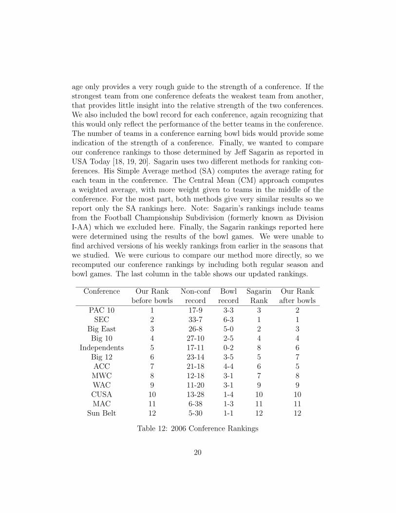
age only provides a very rough guide to the strength of a conference. If thestrongest team from one conference defeats the weakest team from another,that provides little insight into the relative strength of the two conferences.We also included the bowl record for each conference, again recognizing thatthis would only reflect the performance of the better teams in the conference.The number of teams in a conference earning bowl bids would provide someindication of the strength of a conference. Finally, we wanted to compareour conference rankings to those determined by Jeff Sagarin as reported inUSA Today [18, 19, 20]. Sagarin uses two different methods for ranking con-ferences. His Simple Average method (SA) computes the average rating foreach team in the conference. The Central Mean (CM) approach computesa weighted average, with more weight given to teams in the middle of theconference. For the most part, both methods give very similar results so wereport only the SA rankings here. Note: Sagarin’s rankings include teamsfrom the Football Championship Subdivision (formerly known as DivisionI-AA) which we excluded here. Finally, the Sagarin rankings reported herewere determined using the results of the bowl games. We were unable tofind archived versions of his weekly rankings from earlier in the seasons thatwe studied. We were curious to compare our method more directly, so werecomputed our conference rankings by including both regular season andbowl games. The last column in the table shows our updated rankings.
Conference Our Rank Non-conf Bowl Sagarin Our Rankbefore bowls record record Rank after bowls
PAC 10 1 17-9 3-3 3 2SEC 2 33-7 6-3 1 1
Big East 3 26-8 5-0 2 3Big 10 4 27-10 2-5 4 4
Independents 5 17-11 0-2 8 6Big 12 6 23-14 3-5 5 7ACC 7 21-18 4-4 6 5MWC 8 12-18 3-1 7 8WAC 9 11-20 3-1 9 9CUSA 10 13-28 1-4 10 10MAC 11 6-38 1-3 11 11
Sun Belt 12 5-30 1-1 12 12
Table 12: 2006 Conference Rankings
20
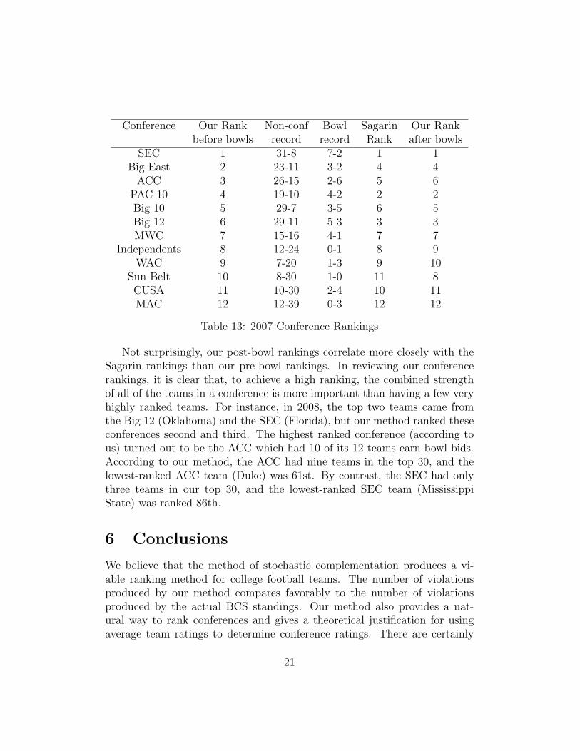
Conference Our Rank Non-conf Bowl Sagarin Our Rankbefore bowls record record Rank after bowls
SEC 1 31-8 7-2 1 1Big East 2 23-11 3-2 4 4
ACC 3 26-15 2-6 5 6PAC 10 4 19-10 4-2 2 2Big 10 5 29-7 3-5 6 5Big 12 6 29-11 5-3 3 3MWC 7 15-16 4-1 7 7
Independents 8 12-24 0-1 8 9WAC 9 7-20 1-3 9 10
Sun Belt 10 8-30 1-0 11 8CUSA 11 10-30 2-4 10 11MAC 12 12-39 0-3 12 12
Table 13: 2007 Conference Rankings
Not surprisingly, our post-bowl rankings correlate more closely with theSagarin rankings than our pre-bowl rankings. In reviewing our conferencerankings, it is clear that, to achieve a high ranking, the combined strengthof all of the teams in a conference is more important than having a few veryhighly ranked teams. For instance, in 2008, the top two teams came fromthe Big 12 (Oklahoma) and the SEC (Florida), but our method ranked theseconferences second and third. The highest ranked conference (according tous) turned out to be the ACC which had 10 of its 12 teams earn bowl bids.According to our method, the ACC had nine teams in the top 30, and thelowest-ranked ACC team (Duke) was 61st. By contrast, the SEC had onlythree teams in our top 30, and the lowest-ranked SEC team (MississippiState) was ranked 86th.
6 Conclusions
We believe that the method of stochastic complementation produces a vi-able ranking method for college football teams. The number of violationsproduced by our method compares favorably to the number of violationsproduced by the actual BCS standings. Our method also provides a nat-ural way to rank conferences and gives a theoretical justification for usingaverage team ratings to determine conference ratings. There are certainly
21

Conference Our Rank Non-conf Bowl Sagarin Our Rankbefore bowls record record Rank after bowls
ACC 1 23-11 4-6 3 1Big 12 2 28-10 4-3 2 3SEC 3 28-11 6-2 1 2
Big East 4 22-12 4-2 5 5Big 10 5 23-12 1-6 6 7MWC 6 19-10 3-2 7 6
PAC 10 7 12-17 5-0 4 4WAC 8 11-19 1-4 9 8
Independents 9 14-26 1-1 10 10MAC 10 14-30 0-5 11 11CUSA 11 11-30 4-2 7 9
Sun Belt 12 10-27 1-1 12 12
Table 14: 2008 Conference Rankings
additional questions that could be investigated. Our experiments involvedthree different parameters: the value of the fixed transition probability p,the value of the weighting factor α for the random transition matrix G, andthe parameter A used in our computation of variable probabilities. Othercombinations of these parameters could easily produce variations on the ba-sic method presented here that might lead to even better performance. Inparticular, it would be of interest to develop other methods of computingvariable transition probabilities that account for factors such as margin ofvictory and home field advantage.
7 Acknowledgements
The authors would like to thank Anjela Govan and Carl Meyer for theircomments and encouragement. Kenneth Massey provided helpful informa-tion about his own ranking method and about the BCS rankings. We arealso appreciative of the data sets provided by James Howell. Finally, wewould like to thank the SUNY Cortland Undergraduate Research Councilfor providing a 2008 Summer Research Fellowship that supported the workof the second author.
22
References
[1] Iqbal Ali, Wade D. Cook, and Moshe Kress. On the minimum violationsranking of a tournament. Management Science, 32(6):660–672, 1996.
[2] BCS standings. http://www.bcsfootball.org/bcsfb/standings.
[3] Abraham Berman and Robert J. Plemmons. Nonnegative Matrices inthe Mathematical Sciences, volume 9 of Classics in Applied Mathematics.Society for Industrial and Applied Mathematics, Philadelphia, PA, 1994.
[4] W. N. Colley. Colley’s bias free college football ranking method: TheColley matrix explained. http://www.colleyrankings.com/matrate.pdf,2002.
[5] A. Govan, C. D. Meyer, and R. Albright. Generalizing Google’s PageR-ank to rank National Football League teams. In Proceedings of the SASGlobal Forum 2008, 2008.
[6] James Howell. James Howell’s College Football Scores.http://homepages.cae.wisc.edu/ dwilson/rsfc/history/howell/.
[7] L. R. Ford Jr. Solution of a ranking problem from binary comparisons.American Mathematical Monthly, 64(8):28–33, 1957.
[8] James P. Keener. The Perron-Frobenius theorem and the ranking offootball teams. SIAM Review, 35(1):80–93, 1993.
[9] Amy N. Langville and Carl D. Meyer. Google’s PageRank and Beyond:The Science of Search Engine Rankings. Princeton University Press,Princeton, NJ, 2006.
[10] Kenneth Massey. Statistical models applied to the ratingof sports teams. Master’s thesis, Bluefield College, 1997.http://www.masseyratings.com/theory/massey97.pdf.
[11] Kenneth Massey. College Football Ranking Comparison.http://www.masseyratings.com/cf/arch/compare2006-14.htm, 2006.
[12] Kenneth Massey. College Football Ranking Comparison.http://www.masseyratings.com/cf/arch/compare2007-14.htm, 2007.
23

[13] Kenneth Massey. College Football Ranking Comparison.http://www.masseyratings.com/cf/arch/compare2008-15.htm, 2008.
[14] Kenneth Massey. College Football Ranking Summary.http://www.masseyratings.com/cf/compsum.htm, 2009.
[15] Carl D. Meyer. Stochastic complementation, uncoupling Markov chainsand the theory of nearly reducible systems. SIAM Review, 31(2):240–272, 1989.
[16] L. Page, S. Brin, R. Motwani, and T. Winograd. The PageRank citationranking: bringing order to the web. Technical report, Department ofComputer Science, Stanford University, 1998.
[17] C. Redmond. A natural generalization of the win-loss rating system.Mathematics Magazine, 76(2):119–126, 2003.
[18] Jeff Sagarin. Jeff Sagarin NCAA Football Ratings.http://www.usatoday.com/sports/sagarin/fbc06.htm, 2007.
[19] Jeff Sagarin. Jeff Sagarin NCAA Football Ratings.http://www.usatoday.com/sports/sagarin/fbc07.htm, 2008.
[20] Jeff Sagarin. Jeff Sagarin NCAA Football Ratings.http://www.usatoday.com/sports/sagarin/fbc08.htm, 2009.
24