a manual for the maps software package · 2019-03-18 · a manual for the maps software package...
TRANSCRIPT
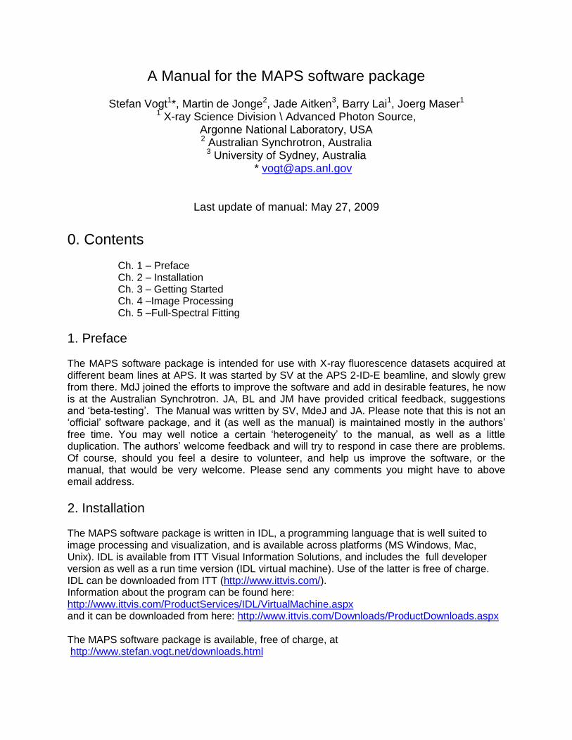
A Manual for the MAPS software package
Stefan Vogt1*, Martin de Jonge2, Jade Aitken3, Barry Lai1, Joerg Maser1 1 X-ray Science Division \ Advanced Photon Source,
Argonne National Laboratory, USA 2 Australian Synchrotron, Australia
3 University of Sydney, Australia * [email protected]
Last update of manual: May 27, 2009
0. Contents
Ch. 1 – Preface Ch. 2 – Installation Ch. 3 – Getting Started Ch. 4 –Image Processing Ch. 5 –Full-Spectral Fitting
1. Preface The MAPS software package is intended for use with X-ray fluorescence datasets acquired at different beam lines at APS. It was started by SV at the APS 2-ID-E beamline, and slowly grew from there. MdJ joined the efforts to improve the software and add in desirable features, he now is at the Australian Synchrotron. JA, BL and JM have provided critical feedback, suggestions and ‘beta-testing’. The Manual was written by SV, MdeJ and JA. Please note that this is not an ‘official’ software package, and it (as well as the manual) is maintained mostly in the authors’ free time. You may well notice a certain ‘heterogeneity’ to the manual, as well as a little duplication. The authors’ welcome feedback and will try to respond in case there are problems. Of course, should you feel a desire to volunteer, and help us improve the software, or the manual, that would be very welcome. Please send any comments you might have to above email address.
2. Installation The MAPS software package is written in IDL, a programming language that is well suited to image processing and visualization, and is available across platforms (MS Windows, Mac, Unix). IDL is available from ITT Visual Information Solutions, and includes the full developer version as well as a run time version (IDL virtual machine). Use of the latter is free of charge. IDL can be downloaded from ITT (http://www.ittvis.com/). Information about the program can be found here: http://www.ittvis.com/ProductServices/IDL/VirtualMachine.aspx and it can be downloaded from here: http://www.ittvis.com/Downloads/ProductDownloads.aspx The MAPS software package is available, free of charge, at http://www.stefan.vogt.net/downloads.html

After installing IDL, place the library files (xrf_library.csv, henke.xdr, compound.dat) into the IDL library path, which should point to something like (on a windows machine) C:\Program Files\ITT\IDL70\lib Please note, it is CRITICALLY important that your data all resides in directories that do NOT contain any white space or wild card characters (such as *, etc). This means, it is NOT a good idea to place the data files into directories like ‘C:\Documents and Settings’.
3. Getting started: On windows, MAPS is typically started by double clicking the file called maps.sav, alternatively, you can start the IDL virtual machine, and then open the maps.sav file. After starting MAPS, two windows will pop up. In Fig. 1 the initialization window is shown.
Fig.1: Initialization window of MAPS. The initialization window can be used to change the main (parent) directory to where the data resides. It is strongly recommended that the following directory/file structure is followed: define as a parent directory the directory above the mda directory. Within this directory, typically the img.dat, rois, output subdirectories reside. The mda directory contains typically the ‘raw’ acquired data. The img.dat directory contains the processed data files, the rois directory is the best place where to save spatial rois the user of this software can define to extract average

spectra from specific areas of the acquired data sets. Output is the directory where MAPS will place most automatically generated output. An image with such a typical directory structure is shown in Fig. 2.
Fig.2: Typical suggested directory structure.
In this example here one would use the ‘press to change directory’ button to change into the Your_Experiment_Name directory, and then press the O.K. button. Please note, that there is a built in help for most of the buttons of the user interface. When hovering with the mouse over a button, text messages will appear on the main MAPS screen.
The Main MAPS window / interface: The Main MAPS window is the place to load scans, and open up specific tools to visualize or work with your data. A Picture of the layout can be seen in Fig. 3.
Fig.3: The main MAPS window. The first pull down menu (displayed here with the text ROI sum) allows you to choose (where applicable) the processing that was done to map elemental content. Typical choices include ROI sum, background subtracted, fitted, etc. The second pull down menu (displayed here with DS-IC) allows one to choose quantification & normalization with the down stream ion-chamber (DS-IC, after the sample), the upstream ion-chamber (US-IC, in front of the sample), current (synchrotron current), or ‘1’, which will display the elemental content in counts/s in the multi element window. The third pull down menu (empty in this Fig), will display the currently loaded file(s), you can switch from one to another by pulling the menu down, and choosing a new file, or by using the ‘<’ and ‘>’ buttons to browse through the files. On the right hand side (right of the ‘scan info’ place holder) text will appear to provide some additional information on buttons over which the mouse is hovering. Under the File menu data files can be loaded into MAPS. Open XRF image will allow you to read one, or several (select using the left mouse button keeping ctrl pressed to select specifics, or use mouse click while pressing shift to select all between the two clicks, or use ctrl+A to select all) img.dat files. As indicated above, these files contain processed data generated from the original mda files. It is suggested that these should

usually be used (when available) to visualize the data, as this provides the largest functionality of the software. These files do NOT contain the full spectra, those remain within the mda files. To operate on full spectra, one usually defines area of interestest using the img.dat files, and then MAPS will search for the correct mda file to extract the spectra from. Open mda file will allow one to read in a raw mda file directly. The functionality of MAPS is somewhat limited using this option, but it can be useful, e.g., to read in a file immediately after (or even during) the scan acquisition, when there is no time to convert mda files to img.dat. Open fly scans (all dets) will open a ‘fly scan’ such that differential phase contrast is already calculated, etc. As opposed to the DPC only version, all detectors are read in, which significantly increases memory requirements, but allows one to also view the single channel analyzers, for X-ray fluorescence overviews. Please note, this is still experimental. Open fly scans (DPC only) will open a ‘fly scan’ such that differential phase contrast is already calculated, etc. Only a small subset of the acquired detectors is shown. Please note, this is still experimental. Under the viewing menu, tools can be chosen to visualize the data from the files that have been loaded. The Multi element view tool allows you to display an arbitrary number of detectors or elemental maps. The tool is updating, so that it will automatically update when a new file is loaded, display choice are changed, etc, with the exception of when a new color scale is chosen. In that case, one has to manually press the update button. The first pull down menu of the main MAPS window (see Fig. 3), allows you to choose (where applicable) the processing that was done to map elemental content. Typical choices include ROI sum, background subtracted, fitted, etc. If the data has been fitted on a per pixel basis, fitted is the recommended option.
4. Processing Images with MAPS

Loading Data 1. Open the latest version of maps
2. Navigate to the parent directory where your files are stored (see above picture)
3. Click okay (see above picture)
4. Go to File, Open XRF File, select the first map file from the XRF directory and click
okay
5. Select File, Update List of Current Files from Directory
a. This will load all XRF Files
6. These files will be loaded into the area circled
7. If your data has not been fitted the option on the left will not include fitted data
a. NO results should be analysed closely on data that has not been fitted – that is on
only ROI Sum data
b. If the data has been fitted choose Fitted

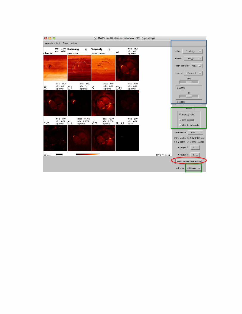
Viewing Data Select View, Multi element view (XS)
Change the Colour o Option, Load Colourtable and select colourtable of interest and select done
o Click update
Change the elements o Once the data has been fitted you will be able to select the elements of interest
o Click Select elements/detectors and select those elements of interest. You can
change the number of elements displayed by varying the “#images x “and “#
images y”
Edit the pictures o To individual pictures:
Select picture by selecting the active picture – this can also be used to
change element
Change the colour scale by adjusting the drag bars which by default are at
100 & 0. Adjusting the bar that is at 100 will change xxx adjusting the bar
that is at 0 will change
Math operations can be performed on individual pictures – eg by dividing
by another element/scatter
o All pictures
Autoscale the pictures on the „full image‟, „centre 1/3 of the image‟ or
„centre 2/3 of the image‟. This will set the maximum and the minimum
for the colour scale based on the region selected
Select XRF log scale or Filter for Autoscale; these will either put a log
scale on the colour scale spreading the colour range; Filter for Autoscale
will remove points of high intensity from the top of the colour range

Printing Pictures In the multi-element window under „Generate Output‟ there are a number of options to export
pictures.
o To export a picture as shown in the image on the screen - Export Auto sized
Image. For all scans – Export Auto Sized Image Series
o To Export individual files for each element – Export Separate Image (8bit gif).
For all scans - Export Image Series 8 bit – gif)
o To Export the full spectra per pixel – export full spectra per pix
Regions of Interest Once the data has been fitted (or even before if you‟re organised enough) you can draw ROIs so
that you can get quantitative results (not yet from the AS) from specific areas of the scan.
Naming
Protocol These can
be done a
number of different ways as outlined below but the most important thing for the person fitting
your data is that the file be called the same as the data filename.roi. If you have more than one
roi per filename that is fine simply name as shown. If the data filename is 2idd_0001.mda then
the roi needs to be called 2idd_0001.roi or for more than one roi 2idd_0001_nucleus.roi
To make the ROIS select the scan of interest then go to Tools, ROI Analysis
To Save o File Save as
o Follow naming convention as above
ROIs can be drawn by hand o Click Draw ROI
o Left click to place a cross to form an outline and Right click to finish.
o Do not click outside the edge of the picture or this will cause a weird ROI to be
formed
o You can clear the selected ROI by completing the ROI (right click) and clicking
clear ROI
o The ROI drawn can be inverted by selecting Invert ROI
o Individual data points can be added by clicking „Start Add Pixels‟
Multiple ROIs o Multiple ROIs for the same scan can be created in a two ways – either by saving
individual files as above or by saving multiple ROIs to the one file

o To save multiple ROIs to the one file:
Simply drag the active ROI bar to the next number and draw a second
ROI.
These ROIs can be copied between ROI number with various
permutations as shown in the copy option (replace existing, AND, OR,
XOR, NOT)
ROIS by cluster analysis o ROIs can be selected by cluster analysis
o Select the number of clusters using the drag bar
o Select the type of cluster analysis:
There are currently several different types of cluster analysis (CA) available to be
used. Generally speaking, we assume a data space spanned by the elements of
interest you choose below. In k-means CA, we take a kartesian coordinate system,
and find cluster centers (up to the number of clusters you chose above) such that
the collective kartesian distance of the data points to „their‟ cluster centers are
minimized. Practically speaking, it attempts to classify the dataset according to
both its elemental composition, as well as its thickness. There a 3 options we have
implemented to use the k-means CA, that differ only in their respective
normalization. Equal weights normalizes each element to reach from 0 to 1,
therefore each picked element has the same weight in the CA. „Weighted by
range‟ normalizes the elements by their range, ie, the difference between
maximum and minimum, whereas „weighted by stddev‟ normalizes the elements
by the standard deviation of their distribution. K-means angular, uses a radial
coordinate system for the cluster analysis. The intent is to avoid classification by
differences in specimen thickness, but instead purely classify by elemental
composition (e.g., do CA based on the relative ratios of Fe, Cu, Zn, irrespective of
the specimen thickness at each point). Only for the angular CA does the factor
pull down menu have significance. The larger its value, the larger an offset will be
applied for a „background‟ region corresponding to „no sample‟, just statistical
noise.
o The elements of interest
o Start cluster analysis
Printing ROIs o To print out a copy of the ROIs to an image file in the multi-element view show
the elements of interest, with the first element of interest selected twice (see above
how to change the elements in an active window)
o Unclick show ROI in all windows so it is only displayed in the first window (for
the element which is shown in the second window as well)
o Output Series – make ROI image series


Quantified Data For data to be quantified the default will be 10keV and with the below list of elements. If your
data was not collected at this energy and/or you are interested in other elements please indicate
so when you supply the data to be fitted as appropriate.
Elements
Si Cr
P Co
S Mn
Cl Fe
Ar Ni
Ca Cu
K Zn
V S_a (scatter)
5. Data Analysis: Full-Spectral Fitting with MAPS
At a fundamental level, MAPS takes as input full-spectrum-per-pixel x-ray fluorescence data,
and enables the user to determine quantitative maps of elemental distribution. After this
processing step (and sometimes beforehand, but please be wary of drawing conclusions from
unfitted data) an ever-increasing number of features / analytical routines can be invoked to
further interrogate the data.
A „simple‟ recipe for MAPS analysis Outline of steps:
1. - Configure MAPS directory structure
- Obtain an ‘appropriate’ version of the file ‘maps_fit_parameters_override.txt’
2. Convert data from .mda format into MAPS custom format (.img.dat)
3. Refine fit parameters (energy calibration, peak shaping, etc) by fitting to a representative
integrated spectrum.
4. Batch process all scans using these parameters.
Detailed steps: 1. The ‘standard’ configuration for maps directories is to have a directory for the experiment, and
within this a directory that contains the .mda files. Prior to running any MAPS analysis this will
look something like (note that /tif, /mca and the logbook file are not related to MAPS

operation):
2. To convert data from .mda to .img.dat:
a. start MAPS by double-clicking the maps.sav file (you will need to download a runtime
version of IDL; see Stefan’s homepage at http://www.stefan.vogt.net/downloads.html)
b. change the parent directory via the front panel so that it points to your data (see below
for example); and then hit ‘O.K. and go to configuration’
c. hit the ‘start processing’ button; this will process all files in the /mda directory. (If your
files are in a different location, or you do not want to process all files, then hit ‘select
NOTE: to view either .mda or .img.dat files you will need either:
(1) to have the maps_fit_parameters_override.txt file in the appropriate location OR
(2) to change the „normalisation‟ field on the MAPS main window to „1‟ (default is „DS-IC‟)

mda files (and directory)’ to choose which files are processed).
d. this will create a directory tree within your parent directory, which will now look
something like:
3. Extract and fit integrated spectrum from a large (and representative) map.
a. Open .img.dat file (also known as ‘XRF image’)
> File > Open XRF image > img.dat directory > (dialogue to select image)
I usually pick a big-ish image, middle to late in the experiment (when experimental
details have settled down!))
b. Confirm image (to ensure that it is a well-behaved scan, worthy of using for calibration)
> viewing > multi element view (M)
if you do not see anything, try playing with ‘select elements / detectors’ to display the
information in your scan.
You may close this window after viewing the data if you wish
c. View integrated spectrum
> viewing > plot integral spectrum

d. Save integrated spectrum
[MAPS: spec tool] > generate output > export raw integrated spectra series (long)
(no confirmation is given)
You probably should close this window after exporting the data
e. Load the data
[MAPS v 1.6.4.3] > Tools > spectrum tool
[MAPS: spec tool] > File > load spectrum > /output > intspec********.img.dat.txt
f. Fit the data
[MAPS: spec tool] > analysis > fit spectrum
[MAPS: spec fit] – change ‘no of iters’ to 50+
[MAPS: spec fit] – hit ‘w/free E, FWHM, tails’
The fit may take some time. Judicious choice of max / min energy may help to speed
this up.
g. IF YOUR FIT LOOKS GOOD – close [MAPS: spec fit] and [MAPS: spec tool] windows and
move to step i.
h. IF YOUR FIT DOES NOT LOOK GOOD – try to identify the cause of the problem;
Are elemental peaks missing?
Is the energy scale a long way off (do the MAPS-designated peak locations line up with
the observed peaks)?
You can test the initial fit parameters by setting the ‘no of iters’ to 0 and doing a fit; are
they approximately correct?
All fit parameters are set in ‘maps_fit_parameters_override.txt’ (be careful to preserve
the formatting within this file! Perhaps take a backup (with suffix .OLD or .ORIGINAL) to
enable easy recovery from mistakes!). If you have trouble with this step (it takes some
experience, so do not hesitate) then see the ‘Further assistance’ section, below.
i. Rename the override files: change the names FROM – TO as indicated below
FROM: maps_fit_parameters_override.txt TO:
maps_fit_parameters_override_input.txt
FROM: average_resulting_maps_fit_parameters_override.txt TO:
maps_fit_parameters_override.txt
when you have done this, the newly calibrated override file will be used to set the
parameters for your per-pixel fits.
4. Commence per-pixel fitting of all spectra
[MAPS v 1.6.4.3] > config + generate maps > general configuration and generate maps
[call maps and general configuration] – check the ‘use fitting’ box
[call maps and general configuration] – start processing (a progress bar will appear)
The fitted results are updated into the .img.dat files for further use.
NOTE: this step will take some time – perhaps around a day – depending on the size and
number of maps being fitted.
Further assistance

The MAPS package is written and maintained by Stefan Vogt of the APS beamline 2-ID-E
([email protected]). If you have any questions that extend beyond the terms of reference of
these notes, please contact your beamline scientist as a first resource, and Stefan only after
exhausting that avenue. Created: 13 Mar 2009 - MdJ
Modified: Mar 2009 - MdJ, SV