a machine learning system for glaucoma detection using
TRANSCRIPT

West Chester University West Chester University
Digital Commons @ West Chester University Digital Commons @ West Chester University
West Chester University Master’s Theses Masters Theses and Doctoral Projects
Summer 2020
A Machine Learning System for Glaucoma Detection using A Machine Learning System for Glaucoma Detection using
Inexpensive Machine Learning Inexpensive Machine Learning
Jon Kilgannon [email protected]
Follow this and additional works at: https://digitalcommons.wcupa.edu/all_theses
Part of the Artificial Intelligence and Robotics Commons
Recommended Citation Recommended Citation Kilgannon, Jon, "A Machine Learning System for Glaucoma Detection using Inexpensive Machine Learning" (2020). West Chester University Master’s Theses. 172. https://digitalcommons.wcupa.edu/all_theses/172
This Thesis is brought to you for free and open access by the Masters Theses and Doctoral Projects at Digital Commons @ West Chester University. It has been accepted for inclusion in West Chester University Master’s Theses by an authorized administrator of Digital Commons @ West Chester University. For more information, please contact [email protected].

A Machine Learning System for Glaucoma Detection using Inexpensive Computation
A Thesis
Presented to the Faculty of the
Department of Computer Science
West Chester University
West Chester, Pennsylvania
In Partial Fulfillment of the Requirements for
the Degree of
Master of Science in Computer Science
By
Jon C. Kilgannon
August 2020
© Copyright 2020

Acknowledgements
I would like to thank my wife, Ivy, for her infinite (and much appreciated) patience
throughout my work on this project. Without her support, this would not have been
possible.
I would also like to thank my advisor, Dr. Richard Burns, for his equal patience
and invaluable advice.

Abstract
This thesis presents a neural network system which segments images of the retina to
calculate the cup-to-disc ratio, one of the diagnostic indicators of the presence or continuing
development of glaucoma, a disease of the eye which causes blindness. The neural network
is designed to run on commodity hardware and to be run with minimal skill required from the
user by packaging the software required to run the network into a Singularity image. The
RIGA dataset used to train the network provides images of the retina which have been
annotated with the location of the optic cup and disc by six ophthalmologists, and six
separate models have been trained, one for each ophthalmologist. Previous work with this
dataset has combined the annotations into a consensus annotation, or taken all annotations
together as a group to create a model, as opposed to creating individual models by annotator.
The interannotator disagreements in the data are large and the method implemented in this
thesis captures their differences rather than combining them together. The mean error of the
pixel label predictions across the six models is 10.8%; the precision and recall for the
predictions of the cup-to-disc ratio across the six models are 0.920 and 0.946, respectively.

Table of Contents
List of Tables ............................................................................................................................. i
List of Figures ........................................................................................................................... ii
Chapter 1: Introduction ..............................................................................................................1
1.1. Overview ..........................................................................................................................1
1.2. Glaucoma Detection via the Cup-to-Disc Ratio ..............................................................3
1.3. Outline..............................................................................................................................4
Chapter 2: Related Work ...........................................................................................................6
2.1. Overview .........................................................................................................................6
2.2. Non-Machine Methods of Glaucoma Detection .............................................................6
2.3. Related Machine Learning Work ....................................................................................7
2.3.1. Optical Coherence Tomography ................................................................................10
2.4. Inexpensive Medical Computing ..................................................................................12
2.5. Other Research Uses of the Dataset ..............................................................................14
Chapter 3: Data ........................................................................................................................18
3.1. Cup-to-Disc Ratio .........................................................................................................18
3.2. Extracting Annotations .................................................................................................21
Chapter 4: Neural Network Architecture .................................................................................26
4.1. Image Segmentation......................................................................................................26
4.2. A Brief Primer on Neural Networks .............................................................................27
4.3. Convolutional Neural Networks ...................................................................................31
4.4. U-Net.............................................................................................................................34
4.4.1. U-Net Comparison .....................................................................................................37

4.5. Class Imbalance ............................................................................................................38
4.6. Image Preprocessing .....................................................................................................39
4.7. Hyperparameters ...........................................................................................................42
4.7.1. Network-Scale Hyperparameters ...............................................................................42
4.7.2. Layer-Scale Hyperparameters ....................................................................................45
4.8. Software ........................................................................................................................49
Chapter 5: Results ....................................................................................................................51
5.1. Training .........................................................................................................................51
5.2. Correctness Metrics ......................................................................................................55
5.2.1. Pixelwise Percent Incorrect, Precision, Recall, and F Measure .................................55
5.2.2. Pixelwise Dice Similarity ..........................................................................................60
5.2.3. Pixelwise Jaccard Metrics ..........................................................................................61
5.2.4. C/D Ratio Percent Incorrect, Precision, Recall, and F Measure ................................61
Chapter 6: Ease and Economy of Use......................................................................................64
6.1. Containerization via Singularity ...................................................................................64
6.2. Feasibility of Inexpensive Hardware ............................................................................67
Chapter 7: Conclusion and Further Work ................................................................................70
Works Cited………………………………………………………………………………….73

List of Tables
1. Absolute value of Performance Error for the GlauNet models ....................................... 9
2. Failed and removed annotation captures by annotator out of 163 images .................... 24
3. Number of pixels across Annotator 3’s images, for full-sized images ......................... 40
4. Number of pixels across Annotator 3’s images, for localized images .......................... 42
5. Hyperparameters ........................................................................................................... 49
6. Number of Images per Training and Validation Set by Model .................................... 52
7. Number of Images Tested ............................................................................................. 55
8. Pixelwise Evaluation Metrics by Model ....................................................................... 56
9. Percentage of Pixels Predicted Incorrectly for Single-Class Predictions ..................... 57
10. Mean and median pixelwise Dice similarity coefficients for GlauNet models ............ 60
11. Mean and median pixelwise Jaccard metrics for GlauNet models ............................... 61
12. Definitions of TP, TN, FP, and FN for C/D ratio ......................................................... 62
13. Precision, recall, and F-measure for the cup-to-disc ratio by annotator ....................... 62
14. Number of epochs of training per model ...................................................................... 63
15. Test Machine Specifications ......................................................................................... 67
List of Figures
1. Features of the human eye important to this project ....................................................... 3
2. Example using RIGA image number 333 ..................................................................... 15
3. RIGA fundus image of retina ........................................................................................ 19
4. RIGA annotated image ................................................................................................. 20
5. RIGA fundus image and annotations of the same image by three annotators .............. 21
6. Captured annotation mask............................................................................................. 23
7. Conceptual design of a neural network neuron ............................................................. 27
8. Fully connected neural network design ........................................................................ 27
9. Sample input data: region of interest captured from RIGA MESSIDOR image 193 ... 28
10. Example neural network ............................................................................................... 28
11. CNN convolutional layer .............................................................................................. 32
12. A 3 x 3 pooling operation with a stride of 3 ................................................................. 33
13. GlauNet’s U-Net architecture implementation ............................................................. 35
14. Architecture of GlauNet’s downward blocks ............................................................... 36
15. Architecture of GlauNet’s upward blocks .................................................................... 36
16. Three annotations overlaid to demonstrate interannotator disagreement ..................... 39
17. Graph of Aggregate Correctness by -log10(Learning Rate) & Epoch to 70 Epochs .... 47
18. Graph of Aggregate Correctness by -log10(Learning Rate) & Epoch to 250 Epochs .. 48
19. Idealized region of interest in a fundus image .............................................................. 51
20. Training Performance of Each Model........................................................................... 53
21. Optic Disc Predicted by Model C at Progressive States of Learning ........................... 54
22. Ground Truth Optic Disc Annotation by Annotator 3 .................................................. 54

23. Cup and disc delineated on an idealized fundus image ................................................ 56
24. Annotations, Predictions, Ground Truth, and Differences ........................................... 59
25. Flowchart of GlauNet usage ......................................................................................... 66
26. Mean Time to Process One Image in a Multi-Image Batch.......................................... 68
1
1: Introduction
1.1. Overview
Glaucoma is a disease which causes vision loss due to “damage to the optic nerve head”
(Foster 2002). It is the “second most common cause of blindness and the most common cause of
irreversible blindness worldwide” (Budenz 2013). While the ultimate causes of glaucoma are
not certain, the disease can be detected and its progression can be tracked, among other factors,
by ongoing loss of vision in the patient’s visual field and by observable damage to a portion of
the retina in the rear of the eye called the optic disc (Martus 2005; Tsai 2003).
The focus of this thesis is the detection of changes in structures in the back of the human
eye which can be indicative of the presence of glaucoma. Human specialists can measure these
structures using either hand-tools or dedicated imaging machinery, but it requires
ophthalmological training to discern the location of the structures and to measure them properly.
The system implemented in this thesis, called GlauNet, is a neural network which has been
trained to emulate the retina measurements which would be taken by six different
ophthalmologists.
Negative changes in the visual field of glaucoma patients are observed in 76% of
untreated patients versus 59% of treated patients, so detection and treatment are vital
to maintaining vision (Forchheimer 2011). In the later stages of the disease, the changes to the
eye caused by the progression of glaucoma are permanent and cannot be corrected by medical
intervention (Kessing 2007). Measurement solely of intraocular pressure, a standard measure for
the risk of glaucoma, can fail to detect asymptomatic glaucoma in the earlier stages of the
disease, so it is a net positive if other methods of testing can be used as well (Kessing 2007; Tsai
2005).

2
A method of detecting glaucoma without requiring the presence of a trained medical
professional is vital to discover potential patients in vulnerable or underserved populations. In a
study of 5,603 adult, urban West Africans performed between 2006 and 2008, 6.8% of those
tested were diagnosed with glaucoma, and 2.5% were already blind. Only 3.3% of those who
had been tested had known they had glaucoma before the diagnosis (Budenz 2013). Primary
open-angle glaucoma is six times more common among African Americans than among white
Americans, and the onset of the disease is a decade earlier. Ophthalmological services are
underutilized even in American urban settings, where health professionals can be found within
close proximity to a prospective patient (Sommer 1991).
An inexpensive method which detects the risk of glaucoma, and which also requires little
or no training, would significantly increase the opportunity for persons in underserved
communities to have potential glaucoma detected and treated. Therefore, one primary design
factor is for GlauNet to run in a timely manner on inexpensive hardware with minimal software
installation required, so all the software which is required to run the network has been packaged
in a container which runs under Singularity, an open-source operating system virtualization
program. Further, the use of mechanical methods of measurement will create uniformity
between measurements, which allows for more precise tracking of the change in measurements
of the eye over time and will thereby lead to better outcomes (Fanelli 2013).
If a disease "has a long preclinical phase with insidious onset, symptomless progression,"
and has many methods of useful treatment, then it is an excellent candidate for frequent and
widespread screening. Glaucoma meets these conditions for screening desirability (Mohammadi
2013), and if a method of screening can be automated, this would make it possible to make
screening more common.

3
1.2. Glaucoma Detection via the Cup-to-Disc Ratio
The optic nerve carries signals
from the retina to the brain. The
portion of the head of the optic nerve
which can be observed on the surface
of the retina is called the optic disc.
The portion of the retina containing
the optic disc can be captured by a
fundus camera to form a fundus
image. The optic disc "contains a
central depression" called the
physiologic cup or optic cup, which is visible on a fundus image as an oval spot, interior to the
optic disc, which is lighter in color than the main body of the disc. Atrophy of the optic nerve
can be observed on the surface of the retina in the form of changes to the shape and relative sizes
of the optic cup and disc, the latter of which can be detected by measurement of the ratio of the
area of the cup to the area of the disc (hereafter the cup-to-disc ratio or C/D ratio) (Tsai 2003;
Foster 2002).
The cup-to-disc ratio was proposed in 1967 as a diagnostic tool for evaluation of the optic
nerve and for communicating its properties (Armaly 1967; Danesh-Meyer 2006). A number of
studies since its proposal have found that the cup-to-disc ratio is among the best predictive
performers among measures of the risk of glaucoma, with an area under the ROC curve of "close
to 0.90," where 1.0 means that a model's predictions are 100% correct (Edward, 2013; Google
Figure 1: Features of the human eye important to this project
Unannotated image by Jordi March i Nogué, made available
under Creative Commons v 3.0

4
2020). The cup-to-disc ratio is among the morphometric variables of the eye which can be used
to diagnose glaucoma, together with the condition of the sectors of the rim area around the optic
cup and parapapillary atrophy (defined as "abnormalities in...the region adjacent to the optic disc
border") (Martus 2005; Wang 2013). Morphometric variables – the shape of formations within
the eye – are often tractable to machine learning procedures.
1.3. Outline
This thesis proceeds as follows:
• In Section 2, an overview of related work is presented. The human-mediated
methods of detecting glaucoma are briefly examined, then previous work in
detecting glaucoma with machine learning is considered. Other work which has
used the same data set as this thesis is also noted. Finally, other inexpensive
medical computing systems are briefly discussed.
• The image data that are used in this project are presented in Section 3. The data
itself are presented, with discussion of the methods that were used by the creators
of the data corpus in annotating the images. The methods used to capture the
annotations from the data corpus’s images are described.
• The architecture of the neural network is described in Section 4. A brief primer of
neural networks is given. U-Net, the specific architecture used in this project, is
explained. Then a severe imbalance among the classes in the annotations is
presented, the reason why this imbalance is an issue for the network is discussed,
and the method used to ameliorate the imbalance is described. Lastly, the process
of deciding what values to use for the network’s hyperparameters is given.

5
• Data on the performance of the neural networks are presented in Section 5. The
process of training the networks and their correctness are described.
• Section 6 describes the design of the Singularity container used to make the
system easier for the user to install and use, and then presents the time required to
run the six networks in Singularity on a cloud instance which duplicates the
specifications of inexpensive hardware.
• The conclusion in Section 7 describes further work which is possible with this
project, and briefly sums up the system’s correctness.

6
2. Related Work
2.1. Overview
A number of machine learning techniques for calculating the cup-to-disc ratio (C/D ratio)
exist; the primary ones focus on either segmentation of a fundus image, or segmentation of an
image captured by Optical Coherence Tomography (OCT), a more complex technology which
captures slices of the retina. The GlauNet project considers fundus images. In machine learning
projects, both fundus and OCT images are segmented either by numerical analysis of the pixels
in the image, or by neural networks analyzing the image in a more complex manner.
This section considers other projects which use the RIGA dataset used to train this
project, and then briefly discusses other projects which utilize or describe inexpensive medical
computing.
2.2. Non-Machine Methods of Glaucoma Detection
Until recently, all tests for the detection of glaucoma were – of necessity – performed by
humans with specialist training. Some methods of glaucoma detection such as gonioscopy,
observation of the point where the cornea and iris meet, have been described as “very much an
acquired art” (Kessing 2007). Several other methods of glaucoma detection require training or
equipment which is not found in the general population, or have inherent uncertainties due to
their methods of operation. Applanation tonometry requires using a small device, after an
anesthetic is applied, to flatten part of the cornea. The device must be kept sterile to prevent the
transfer of infections, and it must be calibrated on an ongoing basis. Pneumatonometry uses a
different small tool, and requires trained skill to read its measurement from a waveform
graph. Stereoscopic optic nerve photography requires the operator to outline the optic disc

7
margin and “center the optic nerve in the image.” The slow scanning speed of Optical
Coherence Tomography, which as mentioned above is a popular source of data for machine
learning work, leads to “motion-induced artifacts” that can make it imprecise. Digital palpitation
requires no equipment, but it requires professional experience as the eye is touched by the
ophthalmologist and the pressure is estimated (Edward, 2013). An automated process would be
valuable, allowing the creation of diagnostic information without the need for specialist
interpretation.
2.3. Related Machine Learning Work
GlauNet captures the cup-to-disc ratio using a U-Net neural network to segment the
fundus image, but other methods for determining the ratio are possible. In 2009, Liu et al
proposed the ARGALI system to automatically calculate the cup-to-disc ratio from a fundus
image. This early system segments the optic disc using eight separate methods. First the disc is
segmented using a level set function, a form of numerical analysis, to separate the image by
analysis of the red channel of the color space. Then an ellipse is fitted around the irregular
region discovered by the level set for half of the disc segmentations. The cup is segmented both
by a level set with thresholding, and by considering the color intensity of the pixels. Half of
these segmentations have ellipses fitted around them as well. The authors state that segmenting
the optic cup is “more challenging than the optic disc segmentation” due to the cup boundary
being less visible than the disc boundary. Eight separate combinations of these methods of
segmentation are fed into a neural network, which creates a prediction based on the eight
segmentations that were fed to it. The predictions made by the neural network are compared
with segmentations made by several ophthalmologists, and those predictions which are within a

8
threshold value of the intra-observer differences are considered to be “within limits” and are
therefore considered a successful segmentation of the image. Ninety percent of the
segmentations were within limits (Liu 2009).
The mean error for GlauNet’s predictions is 10.3%, and the mean correctness of its
predictions 89.7% (see Section 5.2.1). However, this thesis does not define a threshold value as
Liu did; the correctness definition used in this thesis directly compares the predicted class mask
to the ground truth of each individual annotator, and the correctness is the percentage of correctly
labeled pixels in a predicted class mask, or is the proper classification of a C/D ratio as a positive
or negative diagnosis.
In 2015, Nathiya and Venkatesewaran compared several contemporary methods of
segmenting the fundus image to calculate the C/D ratio: Otsu’s image thresholding method,
removal of the blood vessels from the images followed by region growing, hill climbing to find
the seed point for K-means clustering, and fuzzy C-means clustering on the red component of the
color space. They found that the Otsu method, with 11.04% performance error, performed
worst, while fuzzy C-mean clustering was the best with 9.82% performance error (Nathiya
2015). Nathiya defines the performance error percentage in terms of the Experimental C/D ratio
Value (ECV) and the Clinical C/D ratio Value (CCV)1 as:
Performance error (%) = 100 x (ECV – CCV) / CCV
1 ECV, the experimental C/D ratio value, is the value predicted by the model. CCV, the clinical C/D ratio value, is
the value captured from the human annotator’s annotation.

9
The C/D ratio predictions made by the six models in GlauNet were compared to the C/D
ratios captured from the annotations made by their respective six annotators, and the
performance error percentage data has been detailed in Table 1. The mean performance error of
GlauNet is higher than the median performance error due to outliers that pull the mean error
upward. The full ensemble of GlauNet’s models compare roughly well to the methods that
Nathiya surveys, coming in slightly above the Otsu method. However, two of GlauNet’s models
– A and D – perform much better than the others, and in fact perform better than any of the
methods which Nathiya’s team considered.
Similarly to one of the methods Nathiya looked into, Aquino, et al, propose a method for
segmenting the optic disc within a fundus image using Prewett and Otsu edge-detection
techniques on the red and green channel of the color space individually. A Circular Hough
Transform is used to approximate the edges of the optic disc, and then the system chooses the
more successful of the red or green approximations. The authors note that automated
segmentation of the optic disc can be made difficult by the presence of organic irregularities such
as the obscuration of the disc’s rim by blood vessels, or by a small movement of the patient’s eye
creating blurring of the fundus image which is sufficient to cause problems for automated
systems but which human annotators can disregard (Aquino 2010). A Circular Hough Transform
Model Annotator
Mean of
Performance
Error
Median of
Performance
Error
A 1 8.82% 7.01%
B 2 11.18% 9.50%
C 3 14.47% 11.28%
D 4 7.47% 5.36%
E 5 13.96% 7.20%
F 6 14.25% 11.27%
All All 11.89% 8.74%
Table 1: Absolute value of Performance Error
for the GlauNet models

10
was used in a similar fashion by Yin et al, and displayed an average error in area of 10.8%
(Almazroa 2017). GlauNet, in comparison, displays a mean error in area of 10.3% (see section
5.2.1).
2.3.1. Optical Coherence Tomography
A more modern and complex method of detecting the features of the retina than fundus
imaging is Optical Coherence Tomography (OCT), a noninvasive technology which captures
image slices of the retina and allows viewing of the optic disc and cup roughly perpendicular to
the plane of a fundus image and gives a three-dimensional view of the retina (Nathiya 2015,
Khalil 2018). Research into automatically detecting glaucoma from an OCT image has been
limited by the lack of a standard dataset (Khalil 2018). However, attempts have been made with
relatively small OCT image sets. Wu, et al, proposed a method using OCT imaging to segment
the retina into cup, disc, and other. The method de-noises the noisy OCT image, finds a curve
representing the margin between layers of the retina in a 3D image slice, selects points of
maximum curvature on the curve, and defines a ring above those points as the edges of the neural
canal opening in the optic cup; the optic disc is similarly defined. The algorithm ran on “a 3.30
GHz…PC with 16 GB memory” and required 103 seconds to run, while GlauNet was tested on a
2.2 GHz single-core cloud instance with 4 GB of memory and required 60 seconds to run. The
correctness of Wu’s process was measured using the Dice similarity coefficient to be 0.919 ±
0.034 for the measurement of the area of the disc, and 0.928 ± 0.116 for the measurement of the
area of the cup (Wu 2015).
The Dice similarity coefficient was measured for predictions made by each model in
GlauNet (see Section 5.2.2). The mean Dice similarity across all six models for measuring the

11
area of the disc was 0.886, and the model which performs the best on this metric, Model E, has a
mean Dice similarity of 0.907. As a higher Dice metric is better, GlauNet performs slightly
worse than Wu’s process. However, Wu’s method processes OCT images rather than the fundus
images which GlauNet takes as an input, and OCT machines are more expensive than fundus
cameras, which goes against the goals of this project of creating an inexpensive system.
A separate method for determining the cup-to-disc ratio from an OCT image was
described by Ganesh Babu, et al, in 2012. This method detects vertical and horizontal edges in
an OCT image slice via a Haar wavelet transform, then uses this information to find the edge
between the retina and vitreous humor, and the edges of the choroid layer in the retina, which
together help delineate the edges of the optic cup and disc. The authors state the method is
“memory efficient,” but do not quantify the memory used (Ganesh Babu 2012).
In 2015, Ganesh Babu et al discussed a method for segmenting a fundus image, noted
that thresholding techniques alone are not sufficient to segment the optic cup and disc due to
“large [color] intensity variations in the cup region,” and also that the methods they used require
the blood vessels to be removed from the image of the optic cup region by K-means clustering.
Their method, similar to the algorithm of Nathiya and Venkatesewaran referenced above, uses
fuzzy C-mean clustering (FCM), but differs from Nathiya’s method by choosing a form of FCM
which accounts for spatial data to capture information in the relationship between pixels. The
optic disc is approximately located by finding the “brightest point in the green (G) plane of the
fundus image.” The margins of the optic disc and cup are captured by using elliptical fitting
around the rough-shaped clusters discovered by FCM, counting on the fact that the disc and cup
are of a generally elliptical shape. The authors state that the advantages of their method are a

12
smaller mean error than k-Mean or standard FCM, and that the method segments both the optic
disc and cup “in one stage.”
Ganesh Babu’s team also used a back propagation neural network for glaucoma
detection, but instead of using the neural network to segment the fundus, the network is used as a
classifier which is fed the cup-to-disc ratio and two parameters regarding the position of the
blood vessels and the width of the optic disc in the four quadrants of the disc, and outputs a
prediction regarding the patient’s glaucoma status. The neural network classifier was stated to
be 90.7% accurate when its source of data was the information from a fundus image, and 89.27%
accurate when its source of data was an OCT image (Ganesh Babu 2015). To compare, the mean
accuracy for GlauNet, which uses fundus images and bases its diagnosis on a prediction of the
cup-to-disc ratio, is 87.0% (see section 5.2.2).
2.4. Inexpensive Medical Computing
A core intent of this project is to create a system which can be installed and operated
easily by users in economically depressed areas using inexpensive, commodity hardware. Rather
than focusing on lowering the costs to a small-scale end user, much recent research into this field
appears to have been focused on the use of cloud computing to lower the costs of large-scale
medical research, e.g. the cloud computing system for genome sequencing proposed by
Shringarpure et al (Shringarpure 2015). Other research looks to assist patients in remote areas by
proposing telemedicine projects, such as the remote electrocardiogram designed by Hsieh et al,
which allows the gathering of cardiac data remotely (Hsieh 2012). Still further research focuses
on developing ubiquitous medical hardware and software for a first world environment, such as
the smart mirror described and partially implemented by Miotto et al (Miotto 2018). Such

13
systems might be inexpensive in comparison to a full medical suite but are not inexpensive under
the definition intended in this document, which is commodity hardware with 4 GB of memory
installed. We should, however, not focus on these individual projects, which are used for
purposes of illustration, but instead consider the broader issue of affordability in medical
computation.
Presumably, many specialized medical software systems will use cloud computing’s
Platform as a Service and Infrastructure as a Service, rather than Software as a Service, as
medical systems for the most part are not standardized commercial software packages that would
be preinstalled on a cloud system. However, PaaS and IaaS require in-house specialists who can
properly design and implement the cloud system, raising up-front costs (Blanford 2018). And
the cloud time itself can be a significant ongoing expense. Take as an example time purchased
on AWS, the cloud computing infrastructure owned by Amazon. We will consider the least
expensive option, a bare Linux server. The least expensive tier of Linux server which provides
32 GB of memory on AWS costs US$0.301 per hour (Amazon 2020). This is $12.04 each forty-
hour workweek the system is in use. It is, however, unrealistic to expect that a cloud system will
not require extra time to start and to shut down each day, adding to the hours which must be paid
for (Blanford 2018). GlauNet has no continuing costs, as its software is free and open source.
While cloud computing has a relatively small initial cost and a perpetual ongoing cost,
telemedicine has both a significant initial setup cost and an ongoing cost. Training to use a
telemedicine system is required for computer and medical personnel, and can cost between $200
and $2000. Specialized mobile medical devices cost $5,000 to $10,000. The equipment to
support the hardware in the medical office costs $20,000 to $30,000. Telecommunications
software costs between $7,000 and $10,000 per patient to be treated in parallel, and the software

14
costs $1,000 to $1,500 per patient (Escobar 2020). Some telemedicine systems do not feature
cost savings to doctors in their sales pitches, but instead promote the systems as “increasing
productivity and generating new revenue” - patients who can't get to the doctor's office during
normal hours and who would have gone to an alternate medical provider such as an urgent care
clinic will instead contact the doctor via the telemedicine system (Medici 2020). Further,
telemedicine is not a direct replacement for medical professionals, but is instead a force
multiplier. “It is not the intention of telemedicine to reduce the presence of the most valuable
medical resources (physicians and specialists),” writes Aurelian Moraru, “but, on contrary, to use
these scarce and expensive resources in an intelligent manner and time-saving manner” (Moraru
2017).
Lastly, we will consider ubiquitous medical hardware such as the smart mirror proposed
by Miotto. The costs of such systems are difficult or even impossible to discover, as they rely on
hardware which does not yet exist outside of computer labs and which are therefore beyond the
reach of any doctor or patient. GlauNet, in contrast, is designed to run on 15-year-old hardware
using free software.
2.5. Other Research Uses of the Dataset
The Retina Images for Glaucoma Analysis (RIGA) dataset, a collection of fundus images
taken from both male and female patients, was made available in 2018. Most medical data
corpuses are small, or else are not publicly available. The fundus images in the RIGA dataset
were each annotated by six different professional ophthalmologists, marking the locations of the
optic disc and cup. The annotations were made with a stylus on a tablet computer, and saved as

15
images. The RIGA dataset was made available via the University of Michigan’s Deep Blue
system (Almazroa 2018). The dataset is considered in more detail in Section 3.
Almazroa et al extracted the region of interest around the optic disc from RIGA images
and then processed them using a level set function. Almazroa reported that the blood vessels
made the level set calculations “inaccurate,” so the blood vessels were removed from the image
and the image was then “inpaint[ed] using a diffusion process” to infill missing pixels by making
them similar to the surrounding, unremoved pixels. After the image was segmented using the
level set function, the boundaries of the segmentation were “optimized” to create a smoother
contour to the edge. Missing segments of the boundary were then repaired to create a full
segmentation. The images were divided into a set used to validate the model, and a set which
was not used. If standard deviation for the area of the disc annotation for an image was greater
than the mean standard deviation for the areas of all disc annotations, the image was considered
an outlier and was not used for training or validation. Segmentations predicted by the model
were compared to the disc area and centroid, and those that fell outside a given threshold were
marked as incorrect segmentations. The threshold for the MESSIDOR subset of the RIGA
Figure 2: Example using RIGA image number 333
Left: Unannotated image Right: Same image annotated by Annotator 4

16
dataset was 1500 incorrect pixels in area or 3 pixels offset for the centroid. The trained model
was determined to be 86.6% accurate in calculating the disc area on average across all six
annotators (Almazroa 2017). GlauNet is 89.7% accurate on the same measure (see Section
5.2.1).
In 2019 the team of Yu et al used the RIGA dataset as part of the data used to train a U-
Net, the same architecture used for this project. As was done in this project and in the network
trained by Almazroa, a region of interest was selected surrounding the optic disc and used as the
training data. However, Yu’s team chose to use a ResNet34 model with pre-trained weights as
an encoder instead of starting de novo with a fully untrained network as was done in GlauNet.
The authors note that their network, using a pre-trained ResNet encoder, trains in two hours
versus the ten hours required to train a network from scratch. ResNet is often used to handle the
vanishing gradient problem (Dwivedi 2019). The Yu neural network also used 7x7
convolutional layers rather than the smaller 3x3 layers used in GlauNet which capture smaller
features.
After being trained, Yu’s network outputs “blobs” which were then considered as the
segmentation of the image into the cup and disc. This is in contrast to the work I will present in
Section 4 showcasing the network design of GlauNet, which generates a complete or nearly-
complete segmentation of the fundus image and can capture the C/D ratio without further
processing. Further, while GlauNet created six separate models, one for each annotator, Yu’s
team presumed that a pixel was labeled as “disc” or “cup” only if three of the six annotators
labeled it so, and then created a combined network using this majority-rule technique. Yu
considered the segmentation task “as a pixel-level classification problem” and therefore “use[d]
binary cross entropy logistic loss as the loss function.” My network, in contrast, considers the

17
segmentation task as a problem of classifying two disjoint sets, and therefore uses the Jaccard
Distance as its loss function.
Yu’s model was trained for 30 epochs, while the six models that make up the trained
networks in GlauNet were trained for between 847 and 1444 epochs. Yu’s team reported an
average Jaccard Index2 of 94.80% for segmentation of the disc and 79.40% for segmentation of
the cup (Yu 2019). The Jaccard indices for the segmentations by GlauNet’s models were
calculated, as well as the index for the networks as an aggregate (see Section 5.2.3).
The best GlauNet model overall, Model A, has a mean Jaccard Index of 91.20% for the
area of the optic disc and 81.26% for the area of the cup. This is roughly equivalent to Yu’s
method, which is slightly better at this metric for the area of the disc and slightly worse of the
area of the cup. The overall GlauNet model has a mean Jaccard Index of 90.59% for the area of
the disc and 75.85% for the cup. This is noticeably worse than Yu’s method. However, as
noted, Yu’s team created aggregate segmentations and trained against them, which artificially
changes the problem.
The next section discusses the RIGA dataset and the work done to prepare it to use in
training a neural network.
2 The Jaccard Index measures how closely two sets intersect, and is detailed further in section 4.7.1.

18
3. Data
3.1. Cup-to-Disc Ratio
The normal optic disc is approximately 1.5 mm in diameter (Fanelli 2013) and the disc
can vary in area from 1.25 to 4.0 square millimeters in area, with the mode being between 2.0
and 2.25 square millimeters (Hayamizu 2013). The ratio of the diameters of the cup and the disc
is a valuable parameter for diagnosis of glaucoma in both the early and the late stage of the
disease, because the cup-to-disc ratio in glaucomatous eyes is significantly larger than is found in
non-glaucomatous eyes. Furthermore, the cup-to-disc ratio is larger in eyes that present with late
stage glaucoma than in eyes with early stage glaucoma, which allows for tracking the process of
the disease over time (Okimoto 2015).
As previously stated, the cup-to-disc ratio is among several morphometric variables of
the eye which can be used to diagnose glaucoma, and these morphometric variables are
difficult for even trained specialists to determine with precision. Almazroa at al considered six
trained ophthalmologists who annotated the optic cup and disc on identical sets of fundus
images, with agreement of the area of the optic disc, the centroid of the optic disc, and the C/D
ratio considered “by comparing the analysis of each observer with the median result of the other
five,” and with annotations which were beyond the mean standard deviation discarded as
outliers. Almazroa found agreement among the six annotators’ measurements, which had
already been chosen for similarity by removing outliers, was at best 63.4% (Almazroa 2017). An
untrained annotator would be expected to perform even worse than this, which leads to an
obvious issue in areas of the world which are underserved by medical professionals.
To measure the cup-to-disc ratio, one must first detect the cup and the disc, which entails
segmenting the retina in the back of the eye into three classes: the cup, the disc, and what we will

19
call the background - all other features in the retina. The cup-to-disc ratio can then be calculated
using these features.
Automating this
process requires a corpus of
images which have been
manually annotated by
specialists. Such a manual
annotation is possible using
fundus images, which are
images of the retina in the
back of the eye, captured
with the eye either dilated or undilated. Figure 3 shows an example of such a fundus image. The
optic disc is within the pale region, center-right, and the optic cup is inside the optic disc but is
not easily separated by an untrained person; Figure 3 shows the separation by a trained
ophthalmologist.
Fortunately, such a corpus of annotated fundus images exists, the Retinal fundus Images
for Glaucoma Analysis (RIGA) dataset (Almazroa 2018). The dataset consists of 750 images of
varying dimensions ranging from 1440x960 to 2743x1936 pixels. The images are in three sets,
based on which medical center the images were sourced from. The smallest set, from the
Magrabia medical center, was not used as its images are cropped from the full fundus image.
The second-smallest set, from the Bin Rushed medical center, were in lossy jpeg format and
were unsuited to the method used to capture the annotations. The largest set, consisting of
lossless tiff images sourced from the Messidor center, was used. The Messidor images which
Figure 3: RIGA fundus image of retina

20
were 1440x960 were chosen, giving 163 fundus images and 978 annotated images, each 9.8 MB
in size.
The RIGA dataset consists of sets of seven images: one "base" fundus image which
captures the unannotated retina, and six annotated images, one for each ophthalmologist. The
annotations take the form of thin lines which outline the edge of the cup and the disc as
determined by the annotator. The cup and the disc are both marked on the same image, making
it necessary to differentiate them before segmentation could proceed.
Each image in the
RIGA dataset has been
manually annotated by “six
experienced
ophthalmologists
individually using a tablet
[computer] and a precise
pen.” An example of an
annotated image is shown
in Figure 4. The six annotators were not in agreement with one another as to the extent or
location of the cup or the disc. This interannotator disagreement is, however, not at all unusual;
two ophthalmologists can disagree regarding these parameters since the positions of the edges of
the cup and the disc are subjective measures which can be interpreted differently between
annotators (Fanelli 2013). Figure 5 presents the region of interest around the optic cup and disc
Figure 4: RIGA annotated image

21
in RIGA MESSIDOR image 200, and the annotations by three of the ophthalmologists, to
illustrate the disagreement among them.
Almazroa, et al, considered the accuracy of the six annotators in the RIGA dataset. They
defined accuracy to be an annotation whose standard deviation falls within the mean standard
deviation among the all annotated images the authors surveyed. They found that, in the RIGA
dataset, the best accuracy by any of the six annotators was 88.7%, and the lowest accuracy was
75.7%. Annotation of the optic disc by the six annotators was notably better than their
annotation of the cup, “due to the clarity of the disc boundaries” (Almazroa, 2016).
3.2. Extracting Annotations
RIGA is encoded as TIFF images. A TIFF image consists of a three-dimensional array in
which two dimensions of the array are the X and Y coordinate plane of pixels in the image itself
and the third dimension is a set of three integers which represent the coordinate of a pixel's color
in RGB space, with zero being the absence of a given color and with [0,0,0] therefore being
black.
The virtual pens used by the annotators were not all the same color, so it was not possible
to simply search for pixels containing the vector for the annotation color and separate them out to
Figure 5: RIGA fundus image and annotations of the same image by three annotators

22
discover the annotations. Instead, to separate the annotations for the cup and the disc, a program
was written in Python which opens an annotated image and an unannotated base image, converts
them to NumPy arrays using the Pillow image-processing library, and then subtracts the
unannotated base image from the annotated image element-wise. This leaves the annotations as
the difference, and all other pixels as black. Because both the base and annotated images are
lossless TIFFs, there is no artifacting left behind to confuse the process. The algorithm is
presented in Algorithm 1:
for each fundus image:
for each annotator:
img_fundus open fundus image
img_annotation open related annotated image
fundus convert img_fundus into NumPy array
annotation convert img_annotation into NumPy array
diff_tmp pixelwise subtract annotation from fundus
diff sum color space in each pixel of diff_temp
outer_top index of first row with non-zero data
outer_bottom index of last row with non-zero data
outer_left index of first column with non-zero data
outer_right index of last column with non-zero data
center_pt ([outer_left+outer_right]/2 ,
[outer_top+outer_bottom]/2)
append these outer points to outer_list
rotate image around center_pt
discover new outer points, append to outer_list
set elements within n of each point in outer_list to 0
inner_top index of first row with non-zero data
inner_bottom index of last row with non-zero data
inner_left index of first column with non-zero data
inner_right index of last column with non-zero data
append these inner points to inner_list

23
center_pt ([inner_left+inner_right]/2 ,
[inner_top+inner_bottom]/2)
rotate image around center_pt
discover new inner points, append to inner_list
export inner_list and outer_list to R to create bitmap
encoding the captured annotations
Algorithm 1: Capturing annotations from human-annotated images
Due to TIFF using a vector of three integers to define a location in its color space, and
black being [0,0,0], it is possible to add together the three integers of the RGB vector into a
single integer, after which we will find that a black pixel will be represented by zero and all non-
black colors will be represented by positive integers. This allows simple logical processing to
find the edges of the annotations - we find columns and rows which contain non-zero integers,
then find the minima and maxima for the row and column coordinates. A row minimum is the
top of a given annotation's bounding box, while a row maximum is the bottom of the bounding
box. Similarly, column minima and maxima locate the left and right edges of the bounding box,
respectively.
The center of the
annotation is located using
the averages of the row and
column minima and
maxima, then the entire
image is iteratively rotated
around this center. The
row and column maxima
and minima are found
Figure 6: Captured annotation mask
Black: background; Red: optic disc; Green: optic cup
24
along the row and column of the center point at each rotation, which allows us to find points
along the annotation that define it as a polygon of similar shape to the original manual
annotation. After the program captured the annotation marking the greatest extent of the optic
disc, the annotation for the optic disc was removed from the in-memory copy of the annotation
image and the process was repeated to locate a polygon contiguous with the annotation of the
extent of the optic cup.
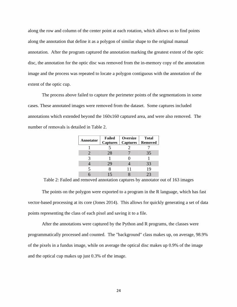
The process above failed to capture the perimeter points of the segmentations in some
cases. These annotated images were removed from the dataset. Some captures included
annotations which extended beyond the 160x160 captured area, and were also removed. The
number of removals is detailed in Table 2.
The points on the polygon were exported to a program in the R language, which has fast
vector-based processing at its core (Jones 2014). This allows for quickly generating a set of data
points representing the class of each pixel and saving it to a file.
After the annotations were captured by the Python and R programs, the classes were
programmatically processed and counted. The "background" class makes up, on average, 98.9%
of the pixels in a fundus image, while on average the optical disc makes up 0.9% of the image
and the optical cup makes up just 0.3% of the image.
Annotator Failed
Captures
Oversize
Captures
Total
Removed
1 5 2 7
2 28 7 35
3 1 0 1
4 29 4 33
5 8 11 19
6 15 8 23
Table 2: Failed and removed annotation captures by annotator out of 163 images

25
The next section introduces neural networks, and presents a system that automatically
learns how to identify a cup and disc, when given data from this section as input. Overall, 860
images will be passed to this next module.

26
4. Neural Network Architecture
In this section, I present an introduction to image segmentation, conventional neural
networks, convolutional neural networks, and U-Net. I describe an issue with class imbalance in
the dataset and how it was corrected by capturing a region of interest in the images around the
optic cup and disc.
4.1. Image Segmentation
To make decisions or judgements regarding medical images, one often must first separate
the areas of interest from the background and from each other, a process called image
segmentation (Bankman 2009). In image segmentation, a process - carried out either by humans
or machines - splits an image up into “meaningful but non-overlapping regions” (He 2018).
Image segmentation can be manual, semiautomatic, or automatic, in a spectrum from a
workflow which requires human work at every step to a workflow in which a computer system
takes in unsegmented data and outputs segmented data. Segmentation can also be divided into
region segmentation and edge-based segmentation; in region segmentation, the system searches
for regions which match “a given homogeneity criterion,” whereas edge-based segmentation
discovers edges between regions where the regions have sufficiently different attributes
(Bankman 2009). The method discussed in this work is semiautomatic and regional.
27
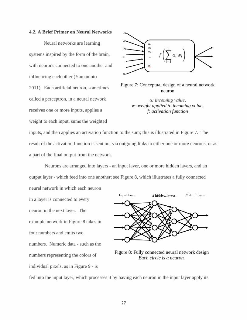
4.2. A Brief Primer on Neural Networks
Neural networks are learning
systems inspired by the form of the brain,
with neurons connected to one another and
influencing each other (Yamamoto
2011). Each artificial neuron, sometimes
called a perceptron, in a neural network
receives one or more inputs, applies a
weight to each input, sums the weighted
inputs, and then applies an activation function to the sum; this is illustrated in Figure 7. The
result of the activation function is sent out via outgoing links to either one or more neurons, or as
a part of the final output from the network.
Neurons are arranged into layers - an input layer, one or more hidden layers, and an
output layer - which feed into one another; see Figure 8, which illustrates a fully connected
neural network in which each neuron
in a layer is connected to every
neuron in the next layer. The
example network in Figure 8 takes in
four numbers and emits two
numbers. Numeric data - such as the
numbers representing the colors of
individual pixels, as in Figure 9 - is
fed into the input layer, which processes it by having each neuron in the input layer apply its
Figure 7: Conceptual design of a neural network
neuron
α: incoming value,
w: weight applied to incoming value,
f: activation function
Figure 8: Fully connected neural network design
Each circle is a neuron.

28
weights and activation function. The output of each neuron in the input layer is fed to one or
more neurons in the first hidden layer. The neurons in the first hidden layer apply their weights
and activation functions to the inputs from the input layer,
and feed their outputs to the second hidden layer. The
second hidden layer processes the inputs from the first
hidden layer in the same way, then passes it to the output
layer, which processes it. The neurons in the output layer
deliver their outputs out to the outside world as the
prediction from the neural network.
A neural network of more than one layer can represent “any continuous function, and
even discontinuous functions” (Russel 2010). Such networks can discover useful features in an
image by creating feature maps within each hidden layer (Cernazanu-Glavan 2013).
Putting data into the network's input layer and then running the data through the layers of
artificial neurons, leading to an output at the output layer, perhaps a binary classification or a
matrix representing an image segmentation, is called the feed-forward process. For the simple
network illustrated in Figure 10, the inputs are denoted as αn and the outputs are denoted as βn,
Figure 9: Sample input data:
region of interest captured from
RIGA MESSIDOR image 193
Figure 10: Example neural network

29
where n is the number of the neuron taking the input or delivering the output. If the activation
function of neuron n is fn(), and wx,y is the weight given by node x to the input from node y, the
output of each neuron at the output layer can be derived:
β1 = 𝑓1(𝑤1,0𝛼1)
β2 = 𝑓2(𝑤2,0𝛼2)
β3 = 𝑓3(𝑤3,0𝛼3)
The outputs of the input layer are then clearly:
βn = 𝑓𝑛(𝑤𝑛,0𝛼𝑛)
These three outputs act as inputs to the hidden layer. The outputs of neurons 4 and
5 are:
β4 = 𝑓4(𝑤4,1𝛽1 + 𝑤4,2𝛽2 + 𝑤4,3𝛽3 )
= 𝑓4 (∑ 𝑤4,𝑛𝛽𝑛
3
𝑛=1
)
= 𝑓4 (∑[𝑤4,𝑛𝑓𝑛(𝑤4,𝑛𝛼𝑛)]
3
𝑛=1
)
Similarly,
β5 = 𝑓5 (∑[𝑤5,𝑛𝑓𝑛(𝑤5,𝑛𝛼𝑛)]
3
𝑛=1
)
The output from neuron 6 is then:
β6 = 𝑓6(𝑤6,4𝛽4 + 𝑤6,5𝛽5 )
= 𝑓6 ( ∑ 𝑤6,𝑚𝛽𝑚
5
𝑚=4
)

30
= 𝑓6 ( ∑ 𝑤6,𝑚𝑓𝑚 (∑[𝑤𝑚,𝑛𝑓𝑛(𝑤𝑚,𝑛𝛼𝑛)]
3
𝑛=1
)
5
𝑚=4
)
The general formula for the three output neurons in the output layer is:
β𝑟 = 𝑓𝑟 ( ∑ 𝑤𝑟,𝑚𝑓𝑚 (∑[𝑤𝑚,𝑛𝑓𝑛(𝑤𝑚,𝑛𝛼𝑛)]
3
𝑛=1
)
5
𝑚=4
)
The output of the neural network is a vector of all three outputs from the neurons
in the output layer.
Training a neural network is the process of discovering the weights which best
approximate a solution to the problem at hand. After feed-forward, the network can read its
output layer, calculate a loss, and perform back-propagation to correct its weights. In back-
propagation, the network will update the weights on its neurons in an attempt to decrease its loss
and come closer to a correct, generalizable network. To back propagate, the network will run the
feed-forward process; determine the error of its output by comparing the calculated and expected
outputs using a loss function; and perform the feed forward operations backward, during which it
will slightly correct each of the weights. Each update via back-propagation is intended to make
the network's model more correct with respect to the measured loss, although this can fail in the
event of overfitting. When the loss falls below some defined point, or when a given amount of
work has been put into the process of training, the network finishes training and saves off its last
(or, in the case of certain sufficiently advanced training methods, its most correct) network
weights.
The method of backpropagation used today was proposed by Rumelhart, Hinton, and
Williams (Rumelhart 1986). It begins by noting that for a “fixed, finite set of input-output
cases,” which exists for any reasonable machine learning training, the error can be calculated by
comparing the model’s prediction and the ground truth as vectors. For the index of input-output

31
pairs, or cases, c; the index of output units j; the predicted state of output y; and the ground truth
or “desired state” d; they give the error, E, as:
𝐸 = 1
2∑ ∑(𝑦𝑗,𝑐 − 𝑑𝑗,𝑐)
2
𝑗𝑐
In backpropagation we calculate the partial derivative ∂E/∂y for each output unit, giving:
∂E
∂𝑦𝑗= 𝑦𝑗 − 𝑑𝑗
Modern systems supporting neural networks, such as TensorFlow, automate the process
of backpropagation and the correction of weights.
When one attempts to use a neural network to work with image data, the number of
weights rapidly increases; for a 200x200 image with color information stored as red, green, and
blue intensities, a single fully-connected neuron will have 120,000 weights (Li 2020). To solve
this issue, Convolutional Neural Networks were proposed.
4.3. Convolutional Neural Networks
The project at hand involves discovering features in images, which is not a strength of
traditional neural networks. Convolutional neural networks (CNNs), which were developed
from traditional neural networks by LeCun and Simnard and were inspired by the configuration
of an animal's visual cortex, retain the relationships among pixels in 2D or 3D space. This
allows a CNN to discover features within an image (Cernazanu-Glavan 2013, Rezaul 2018)
while decreasing the memory footprint of the network by reducing the number of weights in the
network using weight sharing among kernel filters (Hao 2020).

32
The heart of a CNN is the
convolutional layer. A convolutional layer
uses the outputs from neurons that are
connected to a receptive field – a small,
(usually) square region of the input from
the previous layer. The convolutional layer
calculates a dot product between the
weights of these neurons and the receptive
field. A convolutional layer has three-
dimensional volume; if 64 filters are
chosen for a layer with an n x m spatial
size, the layer will be n x m x 64 (Li 2020).
The convolutional layer consists conceptually of a set of feature maps, each of which is
generated by a kernel filter. The kernel filter is moved across the image stepwise, in effect
"looking" at each segment of the image within its receptive field in turn to search for its given
feature. Each feature map learns to capture an element of an image, such as an edge or a
gradient of color. These feature maps will feed into later layers in the network, allowing the
network to aggregate and capture more and more complex features deeper into itself; the model
thereby discovers low-level features in earlier layers and builds them into high-level features in
later layers. Because feature maps are not fixed to a given point in the input data, they can be
used to recognize a pattern anywhere within an image; in contrast, a traditional neural network
which learns a feature will only detect it in a static position within an image. This allows CNNs
to generalize more correctly than traditional neural networks do (Rezaul 2018)
Figure 11: CNN convolutional layer
Images from Github repository of Stanford CS class CS231n,
made available under the free MIT License.

33
Working between the convolutional layers are pooling layers. These layers decrease the
size of their inputs in the height and width dimensions. A pooling layer does not decrease the
size of its input in the depth dimension. Because the pooling layer outputs less data than it
receives, it lowers the amount of calculation required for the network, and also decreases
overfitting. A pooling layer typically will view a set of pixels and take the maximum value from
among them (Li 2020), as Figure 12 demonstrates.
Figure 12: A 3 x 3 pooling operation with a stride of 3
A version of CNN called U-Net was proposed in 2015 by Ronneberger, Fischer, and
Brox, with the intention that the network would work well for image segmentation tasks
(Ronneberger 2015). A U-Net architecture was used in GlauNet. We will discuss its specific
architecture in the next subsection.
0 0 0 0 1 1 1 0 0
0 0 1 1 3 4 2 1 0
0 2 4 5 6 6 4 2 1
1 3 5 6 7 6 5 3 2
1 2 3 5 4 5 4 4 3
0 2 1 1 2 1 2 3 2
0 1 0 0 0 0 1 2 0
0 0 0 0 0 0 0 0 0
0 0 0 0 0 0 0 0 0
4 6 4
5 7 5
1 0 2
34
4.4. U-Net
The task of segmenting fundus images to capture the locations of the cup and disc
requires precision and speed, and also requires the ability to capture a generalizable model
without the use of immense data corpuses which are not available for this project. Fortunately, a
machine learning architecture which matches these requirements exists: U-Net. The U-Net
design is known to have "high capability for high spatial resolution prediction task[s]" (Chen
2018). The U-Net architecture also allows for training with fewer image samples, as the network
transfers features from the lower levels of the network to higher levels, allowing the use of both
fine detail at the lower levels and semantic features at the higher levels; this helps to overcome a
paucity of training data (Zhang 2017).
At its simplest, a U-Net can be thought of as shrinking the image while capturing fine
shape, color, or position detail, then growing or upsampling the image while capturing semantic
information using the fine detail. A U-Net is formed of successive sets of convolutional layers
and pooling layers which shrink the width and height of the data but increase its depth as we
move deeper into the network. Once the full depth of the network is reached, the network
switches to upsampling and grows the width and height of the network while shrinking its depth,
until the output is the same shape as the original input had been. Data from earlier in the
network are copied forward into later layers, so that features discovered earlier in the process,
when fine details are still available, are not lost to the model (Ronneberger 2015). Thus, location
within the image and semantic context are both captured, which is advantageous for image
segmentation (Alom 2019).

35
We will illustrate a U-Net while describing its implementation in GlauNet. The network
is conceptually made of blocks of convolutional, pooling, upsampling, and dropout layers.3 A
dropout layer randomly sets inputs to zero during training. Inputs which are not changed are
“scaled up…so that the sum over inputs is not changed” (TensorFlow 2020). Dropout was added
to the network to prevent overfitting.
Figure 13: GlauNet’s U-Net architecture implementation
The architecture of GlauNet is pictured in Figure 13. As connections in the network go
“down,” the downsampling makes the data being processed smaller in the x and y directions, and
more filters are added to look for more features. A “skip” connection takes the output from a
3 This base U-Net architecture is by Zhixu Hao (Hao 2018).

36
convolutional layer in each down block is sent over to an up block at the same “level,” where the
down block’s output is concatenated with the up blocks input after upsampling, and the
concatenated data is fed into the up block for processing. This skip connection makes certain
that some fine details are not lost by the downsampling process, as the detail is replicated over to
the up blocks. The “bottom” of the network is two convolutional layers and a 50% dropout
layer. The heaviest dropout is at the bottom, as fine detail has been entirely lost at this level.
The abstracted details from Figure 13 are shown in Figures 14 and 15, below. Figure 14
displays a downward block within GlauNet’s architecture, and Figure 15 shows an upward
block.
Figure 14: Architecture of GlauNet’s
downward blocks
Figure 15: Architecture of GlauNet’s
upward blocks
The downward block takes in an input from a previous block, runs it through a
convolutional layer, then through another convolutional layer. The output of the second layer is
sent both to a “skip” connection to one of the up blocks, and down to a pooling layer. The

37
pooling layer contracts the spatial dimensions (x and y) of its inputs by half. This is fed into a
dropout layer which inactivates 25% of the inputs, and feeds to an output to the next block.
The upward block, shown in Figure 15, takes input and upsamples it. It is possible to use
a simple upsample, such as expanding a single pixel into an identical set of four pixels to double
the size of an image. However, GlauNet uses Keras’s convolutional upsampling layer, which
both upsizes the incoming data and has weights which can be corrected (unlike simple
upsampling, which is non-correctable).
The upsampled data then are concatenated with data from the skip connection to the
down block on the same layer as this up block. This concatenated data is fed through a dropout
layer which inactivates 25% of inputs to the first convolutional layer. The two convolutional
layers process the data, and feed it out to the next block.
The last “block” is the output layer, which presents a 160x160 bitmap predicting where
the optic disc is to be found in the input.
4.4.1. U-Net Comparison
U-Net has disadvantages when compared with other neural networks. It is a quite large
and deep network, leading to an extremely large memory footprint. The saved weights file for
one GlauNet model is 355 MB, and GlauNet uses six such models. Making a prediction with a
U-Net is relatively fast; I demonstrate in Section 6.2 that making predicted segmentations for
each of the six models with the U-Net within GlauNet takes a mean of seven seconds. However,
loading the models into memory so that these predictions can be made takes nearly a minute.
Further, U-Nets can have problems when the segmentable area of a class is small in
comparison to the full size of the image, and for medical image segmentation, tissues which are
38
similar to their surroundings can cause issues for U-Nets (Song 2019).4 The segmentable area
being small in comparison to the full size of the input is a problem of class imbalance, and the
next subsection discusses the actions undertaken to handle this issue.
4.5. Class Imbalance
There is, one must note, a significant imbalance in the number of instances of each class
within a fundus image. The full retina of the adult human eye is 1094 square millimeters in area,
although a fundus camera does not capture an image of the entire retina (Kolb 2017), and as
stated earlier in this section, the optic disc – which is larger than the cup – averages between 2.0
and 2.25 square millimeters in area. This difference in sizes between the physiological regions
leads to a class imbalance in the annotated image.
In a full-sized image, the “background” class makes up, on average, 98.9% of the pixels
in a fundus image, while on average the optical disc makes up 0.9% of the image and the optical
cup makes up just 0.3% of the image. We can see that the number of pixels in the cup class and
the number of pixels in the disc class are very roughly equivalent - within a factor of three - but
the number of pixels in the background class is larger than the number in the cup or disc by
several orders of magnitude. An imbalance between classes negatively impacts the training and
generalization of convolutional neural networks. One method for correcting this imbalance is to
preprocess the data to remove the imbalance by removing instances of the majority class, a
process called undersampling (Buda 2018).
To achieve undersampling and thereby roughly balance the number of pixel instances
belonging to each of the three classes, a localized section of the image was captured, as described
4 In the initial design phase of this project, artificially created random “tricolor flags” were made as an input to a U-
Net, to see how rapidly a U-Net would train and to give a first impression of what learning rate would be required.
39
in Section 4.6. Using the known locations of the annotations, a 160 by 160 pixel section of each
base image and each captured annotation, containing the annotated area, was clipped from the
full TIFF images and annotation files.
This left the number of pixels in each image of each class roughly in balance. The
localized sections of the captured annotations were processed and counted, and the background
accounted for on average 38.7% of the pixels (minimum 16.1%, maximum 57.4%), the optic disc
accounted on average for 46.0% of the pixels (minimum 31.9%, maximum 65.1%), and the optic
cup accounted for 15.3% of the pixels (minimum 4.2%, maximum 28.4%).
The localized images and annotation masks were used to train and validate the network.
4.6. Image Preprocessing
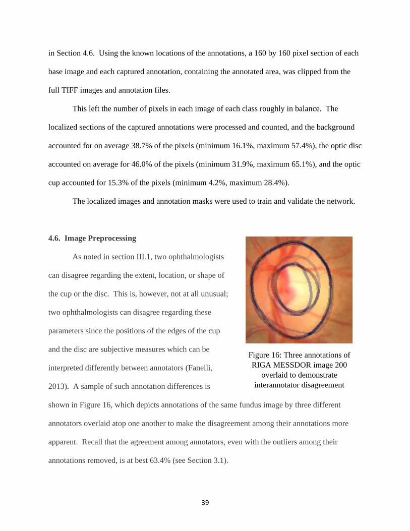
As noted in section III.1, two ophthalmologists
can disagree regarding the extent, location, or shape of
the cup or the disc. This is, however, not at all unusual;
two ophthalmologists can disagree regarding these
parameters since the positions of the edges of the cup
and the disc are subjective measures which can be
interpreted differently between annotators (Fanelli,
2013). A sample of such annotation differences is
shown in Figure 16, which depicts annotations of the same fundus image by three different
annotators overlaid atop one another to make the disagreement among their annotations more
apparent. Recall that the agreement among annotators, even with the outliers among their
annotations removed, is at best 63.4% (see Section 3.1).
Figure 16: Three annotations of
RIGA MESSDOR image 200
overlaid to demonstrate
interannotator disagreement

40
To handle these inter-annotator discrepancies, it was decided to consider the six RIGA
annotators separately, rather than to attempt to build a network which would segment an image
using all the annotators' segmentations as a group corpus, as the use of a group corpus would
lead to a trained network which would not align with any of the annotators.
After the annotations were captured by the Python and R programs, the classes were
programmatically processed and the pixels belonging to each class were counted. Table 3 details
the average number of pixels in each class per image in fundus images annotated by Annotator 3,
and the percentage of the total in each class.
The "background" class makes up, on average, 98.8% of the pixels in a fundus image,
while on average the optical disc makes up 0.9% of the image and the optical cup makes up just
0.3% of the image. We can see that the number of pixels in the cup class and the number of
pixels in the disc class are very roughly equivalent - within a factor of three - but the number of
pixels in the background class is larger than the number in the cup or disc by several orders of
magnitude. An imbalance between classes negatively impacts the training and generalization of
convolutional neural networks. One method for correcting this imbalance is to preprocess the
data to remove the imbalance by removing instances of the majority class, a process called
undersampling (Buda, 2018).
Avg. Pixels
per Image
Minimum
Class
Frequency (%)
Avg. Class Frequency
(%)
Maximum
Class
Frequency (%)
Background 1,366,539.3 98.3 98.8 99.2
Optical Disc 11,948.3 0.5 0.9 1.3
Optical Cup 3,912.4 0.1 0.3 0.5
Table 3: Number of pixels across Annotator 3’s images, for full-
sized images
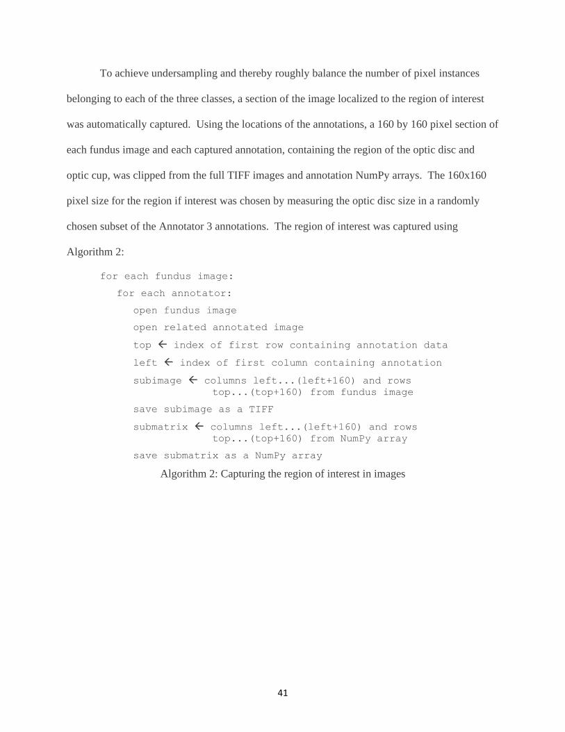
41
To achieve undersampling and thereby roughly balance the number of pixel instances
belonging to each of the three classes, a section of the image localized to the region of interest
was automatically captured. Using the locations of the annotations, a 160 by 160 pixel section of
each fundus image and each captured annotation, containing the region of the optic disc and
optic cup, was clipped from the full TIFF images and annotation NumPy arrays. The 160x160
pixel size for the region if interest was chosen by measuring the optic disc size in a randomly
chosen subset of the Annotator 3 annotations. The region of interest was captured using
Algorithm 2:
for each fundus image:
for each annotator:
open fundus image
open related annotated image
top index of first row containing annotation data
left index of first column containing annotation
subimage columns left...(left+160) and rows
top...(top+160) from fundus image
save subimage as a TIFF
submatrix columns left...(left+160) and rows
top...(top+160) from NumPy array
save submatrix as a NumPy array
Algorithm 2: Capturing the region of interest in images

42
Some regions of interest were more than 160x160 pixels in size, and were removed
during visual checking of the output. Capturing the region of interest around the optic disc left
the number of pixels in each region roughly in balance in each region of interest image. The
number of pixels was counted in those localized images which had been annotated by Annotator
3, and the number of pixels in each class was calculated. The background accounted for on
average 38.3% of the pixels (minimum 12.9%, maximum 57.4%), the optic disc accounted on
average for 46.4% of the pixels (minimum 31.9%, maximum 65.1%), and the optic cup
accounted for 15.3% of the pixels (minimum 4.2%, maximum 23.4%). This is summarized in
Table 4.
The localized images and annotation masks were used to train and validate the network.
4.7. Hyperparameters
4.7.1. Network-Scale Hyperparameters
An untrained neural network is characterized by its parameters and its hyperparameters,
which work together to define how the network will learn, and whether it will learn at all. The
parameters are the settings which are calculated during the learning process, such as weights
within the neuron, while the hyperparameters are those settings chosen by the network’s creator
Avg. Pixels
per Image
Minimum Class
Frequency
(%)
Avg. Class
Frequency (%)
Maximum Class
Frequency
(%)
Background 9,796.9 12.9 38.3 57.4
Optical Disc 11,886.8 31.9 46.4 65.1
Optical Cup 3,916.2 4.2 15.3 28.4
Table 4: Number of pixels across Annotator 3’s images, for
localized images

43
(Alto 2019). A network’s hyperparameters of importance are its activation function, its
initializer, its loss function, its optimizer, and its batch size.
A neuron’s activation function converts the summed weighted inputs of the node into its
output. GlauNet uses the rectified linear unit (ReLU) activation function:
ReLU(x) = {𝑥 𝑖𝑓 𝑥 > 00 𝑖𝑓 𝑥 ≤ 0
GlauNet uses the ReLU activation function both because it has been found empirically to
function well as the activation function for neural networks, and because it is simple and
therefore fast to calculate, which facilitates faster learning (Lu 2019, Arnekvist 2020).
A neural network must be initialized with weights before it begins training. An
incorrectly chosen initializer can cause a network to train more slowly, or entirely fail to train. It
is possible – and was in the past popular – to initialize a neural network with data drawn from
Gaussian distributions with a fixed standard deviation, but this method cannot be used when one
is training a deep network (He 2015). An improperly initialized layer will either diminish or
overamplify the signal fed into it, leading to an incorrectly identified gradient and an incorrect
output (Mishkin 2016). In 2015 He, et al, recommended initializing the weights in a deep neural
network’s neuron by drawing from Gaussian distributions using a standard deviation which
relates to the number of inputs rather than being fixed (He 2005). To make it more likely that the
network will train properly, GlauNet uses this He normal initializer, which is built into
TensorFlow. Note that in TensorFlow it is possible to define an initializer for each layer rather
than for the entire network, but He normalization was used for the entire network for this project
as it is the correct initializer in this application.
Perhaps the most important choice in a neural network is which loss function to use. A
loss function describes how closely a model’s output relates to ground truth, and training a neural
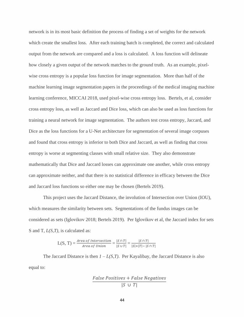
44
network is in its most basic definition the process of finding a set of weights for the network
which create the smallest loss. After each training batch is completed, the correct and calculated
output from the network are compared and a loss is calculated. A loss function will delineate
how closely a given output of the network matches to the ground truth. As an example, pixel-
wise cross entropy is a popular loss function for image segmentation. More than half of the
machine learning image segmentation papers in the proceedings of the medical imaging machine
learning conference, MICCAI 2018, used pixel-wise cross entropy loss. Bertels, et al, consider
cross entropy loss, as well as Jaccard and Dice loss, which can also be used as loss functions for
training a neural network for image segmentation. The authors test cross entropy, Jaccard, and
Dice as the loss functions for a U-Net architecture for segmentation of several image corpuses
and found that cross entropy is inferior to both Dice and Jaccard, as well as finding that cross
entropy is worse at segmenting classes with small relative size. They also demonstrate
mathematically that Dice and Jaccard losses can approximate one another, while cross entropy
can approximate neither, and that there is no statistical difference in efficacy between the Dice
and Jaccard loss functions so either one may be chosen (Bertels 2019).
This project uses the Jaccard Distance, the involution of Intersection over Union (IOU),
which measures the similarity between sets. Segmentations of the fundus images can be
considered as sets (Iglovikov 2018; Bertels 2019). Per Iglovikov et al, the Jaccard index for sets
S and T, L(S,T), is calculated as:
L(S, T) = 𝐴𝑟𝑒𝑎 𝑜𝑓 𝐼𝑛𝑡𝑒𝑟𝑠𝑒𝑐𝑡𝑖𝑜𝑛
𝐴𝑟𝑒𝑎 𝑜𝑓 𝑈𝑛𝑖𝑜𝑛 =
|𝑆 ∩ 𝑇|
|𝑆 ∪ 𝑇| =
|𝑆 ∩ 𝑇|
|𝑆|+|𝑇|− |𝑆 ∩ 𝑇|
The Jaccard Distance is then 1 – L(S,T). Per Kayalibay, the Jaccard Distance is also
equal to:
𝐹𝑎𝑙𝑠𝑒 𝑃𝑜𝑠𝑖𝑡𝑖𝑣𝑒𝑠 + 𝐹𝑎𝑙𝑠𝑒 𝑁𝑒𝑔𝑎𝑡𝑖𝑣𝑒𝑠
|𝑆 ∪ 𝑇|

45
The Jaccard Distance is defined for binary masks, which makes it ideal for the one-vs-
many masks that GlauNet uses (Kayalibay 2017).
The loss function which is chosen for a neural network must be differentiable if a neural
network is to train, and the Jaccard Distance is differentiable. Moreover, for the purposes of the
current image segmentation problem, the Jaccard Distance will “reflect both size and localization
agreement” (Bertels 2019), which is necessary to correctly determine the location of the cup and
disc. Additionally, per Bertels, Jaccard loss has “the most impact for refining the segmentations
of samples of small size,” which is important for medical image segmentation, as medical image
corpuses tend to be relatively small.
Once it is calculated, the loss function must be used to optimize the network, which will
minimize the loss and in principle make the network's learned model more correct. The
stochastic gradient descent (SGD) optimizer is the most popular but it functions properly only
when the learning rate of the network scales inversely with respect to time. The Adam (adaptive
moment estimation) optimizer updates SGD by adapting the learning rate so it scales with the
gradient of the loss (Rezaul 2018). Rezaul reports that Adam "performs well in most
cases." Additionally, Adam allows for batch sizes - the number of images processed by the
network before recalculating the network's weights - to be large or small. To keep the memory
footprint of GlauNet minimal while it is learning, the network’s batch size is 1.
4.7.2. Layer-Scale Hyperparameters
There are three basic hyperparameters for a single convolutional layer: the size of the
kernel, the stride the kernel moves by, and the number of kernels used (Wei 2019). Rather than

46
being found via a search, these hyperparameters were set after considering the needs of the
network.
The kernel used in the network's convolutional layers was the smallest useful kernel
possible: three by three pixels. Smaller kernels were used because larger kernels will "reduce
localization accuracy," according to Ronneberger et al, and the problem at hand requires
carefully localizing any discovered features because we must find very precise edges to the cup
and disc to allow for accurate measurement of the cup-to-disc ratio. Wei et al point out that
smaller kernels allow for more complexity in a network's model than do larger kernels, and
smaller kernels also decrease the number of parameters which decreases the time required to
train a network (Wei 2019).
The stride of the network - the pixel distance a kernel is moved with each step - is one, as
small as possible, so that no detail is missed and no context between features is lost, at the cost of
the network training more slowly. Using a small kernel, which captures even small details, and
moving that kernel as little as possible between iterations, will allow the network to capture
details of the image while still eventually encompassing the entire image.
The number of kernels in each convolutional layer increases by a factor of two with each
level deeper in the network. This is recommended by a number of authors (e.g. Milletari 2016,
Iglovikov 2018, Chen 2018). The initial number of kernels in the shallowest layers was set at 64,
with deeper layers containing 128, 256, 512, and 1024 kernels respectively. These quantities
were chosen because they were large enough to capture significant numbers of features, while
being small enough to fit within a reasonable amount of memory.
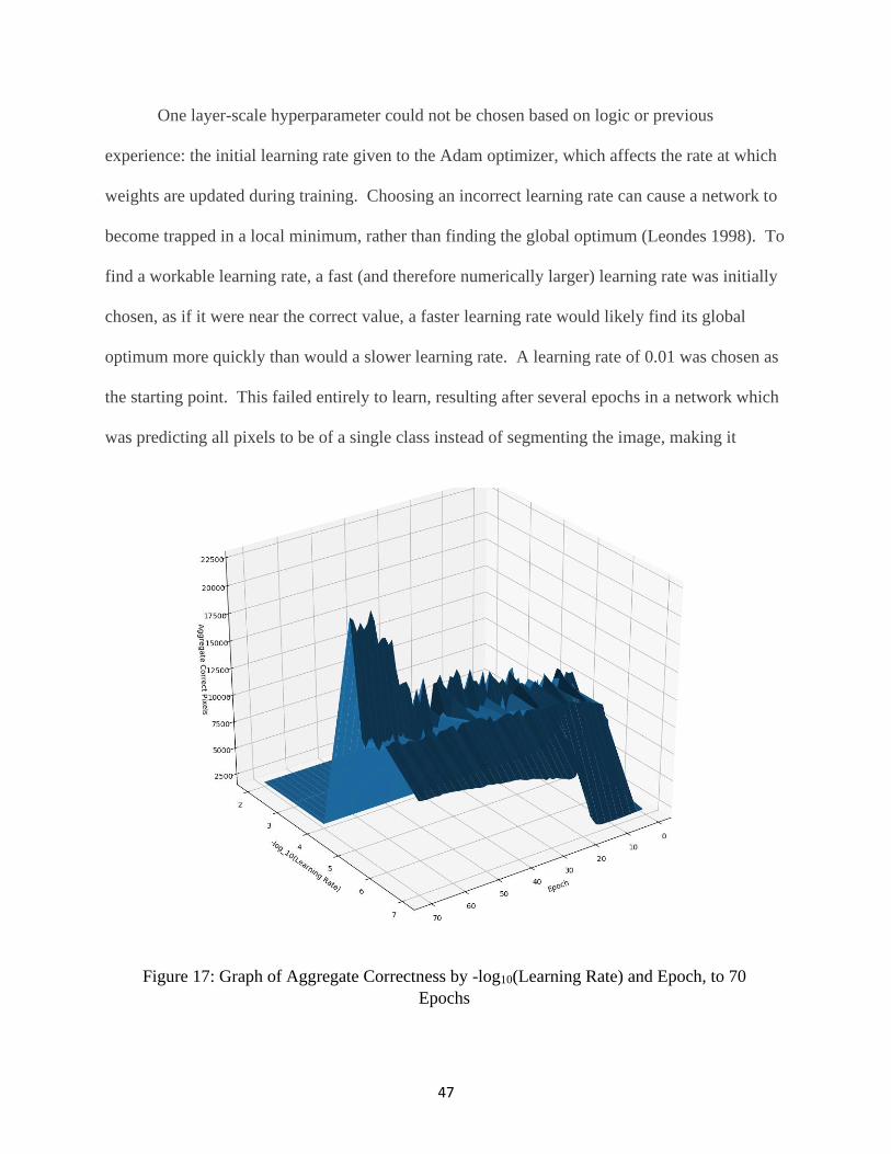
47
One layer-scale hyperparameter could not be chosen based on logic or previous
experience: the initial learning rate given to the Adam optimizer, which affects the rate at which
weights are updated during training. Choosing an incorrect learning rate can cause a network to
become trapped in a local minimum, rather than finding the global optimum (Leondes 1998). To
find a workable learning rate, a fast (and therefore numerically larger) learning rate was initially
chosen, as if it were near the correct value, a faster learning rate would likely find its global
optimum more quickly than would a slower learning rate. A learning rate of 0.01 was chosen as
the starting point. This failed entirely to learn, resulting after several epochs in a network which
was predicting all pixels to be of a single class instead of segmenting the image, making it
Figure 17: Graph of Aggregate Correctness by -log10(Learning Rate) and Epoch, to 70
Epochs

48
entirely useless. The learning rate was iteratively decreased by a factor of 10, and retrained. As
the learning rate was decreased from 0.01 to 0.001, to 10-4, the network continued to converge
into a state which predicted only one class for all pixels. At 10-5, however, the network
converged to a correct prediction.
A second set of test runs was then undertaken; the learning rate of 10-5 was increased and
decreased by a factor of 5, to 5x10⁻⁵ and 5x10⁻⁶, and these new networks were trained to a
minimum of 250 epochs using each learning rate, but this caused the network to again converge
to less correct models than did the 10-5 network.
Figure 18: Graph of Aggregate Correctness by -log10(Learning Rate) and Epoch, to 250
Epochs

49
The graphs Figures 17 and 18 show the networks learning (or failing to learn). The
graphs show learning as aggregate correct pixels, which is the number of correct pixels minus the
number of incorrect pixels; this is a measure of learning which is unfeasible for training a
network, but which is human-understandable. The networks were trained using the Jaccard
Distance, which is described above.
The hyperparameters discussed in this section are summarized in Table 5.
Hyperparameter Value
Activation Function ReLU
Initializer He normal
Loss Function Jaccard Distance
Optimizer Adam
Optimizer Learning Rate 10-5
Kernel Size 3x3
Kernel Stride 1
Number of Kernels 64 - 1024
Table 5: Hyperparameters
4.8. Software
Two major software packages were used in this project: TensorFlow/Keras, and
Singularity.
Singularity5 is a free and open software program which runs containers which contain
virtualized Linux systems. The intention of Singularity is to provide reproducible environments,
compatibility with diverse computational architectures, and the running of software by
“untrusted users running untrusted containers.” This means that a complete Linux environment
can be packaged and ported to a system running Singularity, and that it can be run (and installed,
5 The user documentation for Singularity, including installation instructions, is available at https://sylabs.io/docs/
50
depending on the security rules on the local system) without requiring root or administrator
privileges.
TensorFlow6 is a free and open library designed for differentiation, which is frequently
used for machine learning tasks. TensorFlow underlies Keras,7 which is a free and open source
library specifically for building neural networks.
6 TensorFlow has extensive documentation available at https://www.tensorflow.org/ 7 Documentation available at https://keras.io/

51
5. Results
5.1. Training
A human ophthalmologist separates a fundus image into three separate classes: optic cup,
optic disc, and background. The neural network presented in the previous section was designed
to recognize the optic disc, because the sets of pixels for the cup, disc, and background are
disjoint. Therefore, determining the extent of the optic disc also determines the extent of the
optic cup and the background. This is most easily seen using the idealized fundus image in
Figure 19, in which the optic cup is depicted in red, the optic disc in black, and the background
in blue.
The trained networks therefore segment a fundus image into the optic disc and “other.”
This limits the scope of the problem, and makes training the networks faster without losing any
information.
Six networks were trained from scratch, one for each human annotator in the RIGA
dataset. Each network had the same base architecture, described in the previous sections, but due
to the presence of dropout in the architecture causing randomized neurons to “drop out” of the
network, the finalized architectures will differ on the scale of individual neuron connections.
Figure 19: Idealized region of interest in a fundus image
Blue: background, Black: optic disc, Red: optic cup
Note that, when calculating the areas of a segmentation, the optic
disc is the red and black regions combined.

52
The corpus of training data was split into two sets: roughly 80% training data, and 20%
validation data. The image files contain a serial number which increments by one, so validation
images were chosen by selecting the images whose file number is evenly divisible by five, which
was done to apply an algorithm which gave repeatable numbers. The number of images in each
set is shown in Table 6.
During training, the networks updated their weights against the training data, and then the
validation images were run through the updated network to calculate the loss as a performance
measure. The loss at the end of each epoch was captured, and compiled into graphs to visualize
the learning curve of each model, shown in Figure 20.
Model Annotator
Num. of
Training
Images
Num. of
Validation
Images
A 1 127 29
B 2 102 26
C 3 130 32
D 4 106 24
E 5 114 30
F 6 111 29
Table 6: Number of Images per Training and
Validation Set by Model

53
It is immediately apparent that the loss drops significantly after approximately 50 epochs
of training. The order of the training images was randomized before each training epoch was
run, so the order in which the images were fed into the network during training did not cause this
effect. The sharp drop in the loss is not an error or a flaw in the training; it is due to the network
Figure 20: Training Performance of Each Model
Training loss in black, validation loss in blue.

54
encoding the existence of a hole in the center of the annotation where the optic cup is found. A
series of predictions, shown in Figure 21, was captured which shows this learning process for
Model C, which is learning to predict Annotator 3. The ground truth for Annotator 3 which the
model is attempting to predict is shown in Figure 22.
Figure 22: Ground Truth Optic Disc Annotation by Annotator 3
The network weights which produced the best loss were saved as an ongoing process, so
the final network for each annotator is the one among all the networks trained which provides the
best model for that annotator. When loaded into TensorFlow, each model will predict how an
individual human annotator would have segmented a given fundus image. These six models
were then tested to determine how correct their predictions were.
The training of a neural network is in general a stochastic procedure, so each time a
network is trained de novo the resulting network will be different. This makes it difficult to
Epoch 52 Epoch 54 Epoch 56 Epoch 58
Figure 21: Optic Disc Predicted by Model C at Progressive States of Learning

55
compare the six models on a micro-level, but they remain similar in their overall design, which
was detailed in Section 4.
5.2. Correctness Metrics
After the models completed training, all the
fundus images in the validation data for each annotator
were processed through the system against each of the
six annotators to determine how correct the system
would be. The number of images tested per annotator
is shown in Table 7. Python programs were written
which loaded each annotator’s model in turn and
processed all validation files against that annotator. The training data was not used, as it would
be more likely to be correctly segmented by the network and therefore would bias the
calculations towards finding that the predictions are correct.
5.2.1. Pixelwise Percent Incorrect, Precision, Recall, and F Measure
Note that the area of the disc includes the cup (Almazroa 2016, Almazroa 2017), and in
fact the cup is often called the “cup of the optic disc” (Chakravarty 2017). This is illustrated for
an idealized fundus image in Figure 23. This is important to keep in mind when discussing the
correctness of the segmentation of the disc.
Network Annotator
Num. of
Images
Tested
A 1 29
B 2 29
C 3 30
D 4 24
E 5 30
F 6 29
Table 7: Number of images tested
for correctness

56
The number of pixels which each prediction correctly or incorrectly identified were
counted, and an image was created for each prediction showing where the ground truth and the
predicted segmentation differed. Evaluation metrics were calculated using the predictions and
the ground truth data, which is tabulated in Table 8. The F-Measure is the harmonic mean of
precision and recall.
The pixelwise percent incorrect measure was calculated as follows:
percent incorrect = (false positives + false negatives) / total pixels
For all annotators, the predicted images were incorrect, in the mean, by 10.3%. The
individual annotators varied slightly from this average. Note that Model D, based on Annotator
Model Annotator Percent
Incorrect
Mean
Precision
Median
Precision
Mean
Recall
Median
Recall
Mean F
measure
Median F
Measure
A 1 9.6% 0.8790 0.8924 0.9080 0.9206 0.8909 0.9043
B 2 11.3% 0.8646 0.8879 0.8800 0.9020 0.8683 0.8688
C 3 11.1% 0.8648 0.8826 0.9038 0.9093 0.8816 0.8957
D 4 10.3% 0.8547 0.8613 0.8987 0.9165 0.8738 0.8822
E 5 9.4% 0.9080 0.9135 0.9096 0.9239 0.9068 0.9104
F 6 10.2% 0.8846 0.9123 0.9055 0.9114 0.8923 0.9045
All All 10.3% 0.8768 0.8904 0.9015 0.9138 0.8863 0.8974
Table 8: Pixelwise Evaluation Metrics by Model
Disc and cup Area of disc Area of cup
Figure 23: Cup and disc delineated on an idealized fundus image
Blue: background; Black: disc; Red: cup

57
4, predicts 10.3% incorrect pixels, which is also the mean incorrectness among all predictions by
all the models. This is interesting because Almazroa, et al, report that Annotator 4 “had the best
agreement with all other ophthalmologists in terms of disc area and centroid markings,” which
“means that [he or she] provided good disc boundary markings” (Almazroa 2016). Since Model
D’s predictions are in the middle of the pack, so to speak, it appears to agree in general terms
with the other five models in much the same way Annotator 4’s markings agreed best with their
fellow ophthalmologists’. However, the precision, recall, and F measure for Model D are lower
than the equivalent metrics for all models except for median recall. This implies that Model D is
actually worse at predicting its annotations than average for all models.
To give a baseline, masks which “predicted” all pixels as belonging to the optic disc class
or the non-optic disc class were created, and compared to the validation data for each annotator.
The information is summed up in Table 9.
The models’ predictions in general
captured the shape of the ground truth
annotations, as can be seen in Figure 24.
Each of the annotators has a distinctive
signature to his or her segmentations of the
image which can be seen by a human
observer. For example, annotators 1 and 2
tend to segment the optic disc – the “hole”
in the center of the segment – with a larger area than do annotators 5 and 6. This behavior is
captured by the models, albeit imperfectly. These imperfections are caused, for instance, by the
organic shapes of the blood vessels in the fundus image that could confuse the model, which can
Model Annotator
Percent
Incorrect
if Predict
All Class
0
Percent
Incorrect
if Predict
All Class
1
A 1 44.2% 55.8%
B 2 43.1% 56.9%
C 3 48.2% 51.8%
D 4 41.4% 58.6%
E 5 50.3% 49.7%
F 6 48.2% 51.8%
All All 46.2% 53.8%
Table 9: Percentage of Pixels
Predicted Incorrectly for Single-Class Predictions of
Class 0 (Baseline) or Class 1 (Optic Disc)

58
be seen especially well in Models A, B, and F, for the predicted disc, for this test instance. Note,
for example, the high rate of correctness for Model F in Figure 24, below. These metrics are
good, even though the model has made a serious error in segmenting the optic cup. The model
appears to have been confused by the blood vessel in the lower quadrant of the optic disc.
However, this error is small in area, so it doesn’t change the pixelwise precision or recall by a
large amount. It does, however, make the C/D ratio significantly incorrect.

59
Human Annotation Captured Annotation Prediction Difference
Figure 24: Annotations, Predictions, Ground Truth, and Differences
Fundus image 180
Model A
(Annotator 1)
Model B
(Annotator 2)
Model C
(Annotator 3)
Model D
(Annotator 4)
% Incorrect: 13.5%
Precision: 0.8708
Recall: 0.8506
% Incorrect: 14.8%
Precision: 0.8852
Recall: 0.8366
% Incorrect: 8.5%
Precision: 0.9334
Recall: 0.8968
% Incorrect: 12.9%
Precision: 0.8212
Recall: 0.9005
% Incorrect: 12.6%
Precision: 0.8854
Recall: 0.9103
% Incorrect: 8.0%
Precision: 0.9213
Recall: 0.9302
Model E
(Annotator 5)
Model F
(Annotator 6)

60
5.2.2. Pixelwise Dice Similarity
Per Thada and Jaglan (Thada 2013), the Dice similarity coefficient for sets X and Y is
given by:
Dice(X,Y) = 2 |𝑋 ∩ 𝑌|
|𝑋|+|𝑌|
A program was written in Python to measure the Dice similarity coefficient was
measured for predictions made by each model in GlauNet against the validation set. The results
are summarized in Table 10. A higher Dice coefficient represents a better prediction by the
network. The Dice similarity coefficient is similar to the Jaccard metrics described in the next
subsection; however, unlike the Jaccard Distance, (1 – Dice) does not obey the triangle
inequality. The triangle inequality – the requirement that
dist(x,z) ≤ dist(x,y) + dist(y,z)
– is one of the properties required for a proper distance metric (Ontañón 2020).
Model Annotator Dice coefficient
Mean Median
A 1 0.891 0.904
B 2 0.868 0.869
C 3 0.882 0.896
D 4 0.874 0.882
E 5 0.907 0.910
F 6 0.892 0.904
All All 0.886 0.897
Table 10: Mean and median pixelwise Dice
similarity coefficients for GlauNet models

61
5.2.3. Pixelwise Jaccard Metrics
Using a Python program, the Jaccard Index and Jaccard Distance8 were measured for
GlauNet’s predictions. The results are summarized in Table 11.
The Jaccard Distance was used as the loss function when training the neural networks. A
higher Jaccard Index (or a lower Jaccard Distance) indicates that two sets are more congruent,
and therefore in the case of a neural network, that the prediction is closer to the ground truth.
5.2.4. C/D Ratio Percent Incorrect, Precision, Recall, and F Measure
The range of C/D ratio values which define an eye as glaucomatous or non-glaucomatous
are: less than 0.4 is likely non-glaucomatous, 0.4 to 0.8 can be suspect for early glaucoma, and
greater than 0.8 should be “consider[ed] glaucomatous unless proven otherwise” (Tsai 2005).
Positive and negative predictions, then, are defined in terms of predictions matching or failing to
match the diagnosis for a given annotator. This leads to definitions of true and false negative,
and true and false positive, which are given in Table 12.
8 The Jaccard Index and Distance are explained in Section 4.7.1. Briefly, the Jaccard Index measures the difference
between two sets, and the Jaccard Distance is 1 – (Jaccard Index), used as a loss function.
Model Annotator Disc Cup
Mean Median Mean Median
A 1 91.20 91.96 81.26 83.84
B 2 89.04 89.79 74.59 76.98
C 3 90.43 92.13 72.34 76.27
D 4 91.05 92.15 81.09 82.88
E 5 91.40 91.62 75.55 78.15
F 6 90.34 90.66 71.43 70.75
All All 90.59 91.40 75.85 78.20
Table 11: Mean and median pixelwise Jaccard Index
percentages for GlauNet’s models

62
model
human CDR < 0.4 0.4 ≤ CDR ≤ 0.8 CDR > 0.8
CDR < 0.4 True Negative False Positive False Positive
0.4 ≤ CDR ≤ 0.8 False Negative True Positive False Positive
CDR > 0.8 False Negative False Negative True Positive
Table 12: Definitions of TP, TN, FP, and FN for C/D ratio
A C/D ratio was calculated for each annotator’s segmentation of the fundus image. Then
this C/D ratio was compared to a C/D ratio calculated using the segmentation predicted by the
model trained on that annotator’s work. Precision, recall, and the F-measure were calculated
using the definitions of true/false positives and negatives given in Table 11. The percentage
incorrectness was calculated using the metric which would capture any incorrectness on the part
of the models: to be counted as correct, the model was required to exactly match the diagnosis
based on the human’s annotations; e.g., to be counted as correct when the human diagnosis
would be “suspect for early glaucoma,” the model must predict a C/D ratio between 0.4 and 0.8.
The results of these calculations are summarized in Table 13.
Model Annotator Percent
Incorrect Precision Recall F-Measure
A 1 0.0 1.000 1.000 1.000
B 2 11.5 0.920 0.958 0.939
C 3 21.9 0.885 0.852 0.868
D 4 0.0 1.000 1.000 1.000
E 5 20.0 0.826 0.905 0.867
F 6 21.4 0.875 0.875 0.875
All All 13.0 0.920 0.946 0.933
Table 13: Precision, recall, and F-measure for the cup-to-disc ratio by annotator
There is noticeable variation in the correctness metrics. Models C, E, and F, which are
all 20% or more incorrect and below 0.9 in precision, recall, and F-measure, do remarkably

63
worse than models A and D, which properly predicted all the instances put to them. It is not
clear why this is, but note the number of epochs of training for each model, in Table 14.
Model Annotator Number of Epochs
Spent in Training
A 1 1118
B 2 1049
C 3 874
D 4 1258
E 5 1404
F 6 1444
Table 14: Number of epochs of training per model
Model C trained for notably fewer epochs than did models A and D, while models E and
F trained for notably more epochs than did A and D.9 So perhaps model C is underfitting while
models E and F are overfitting, but more research would be necessary to determine the exact
cause of the difference in the accuracies of the models.
Models C, E, and F do not show this same significant difference in metrics on the
pixelwise measures of accuracy. This is because the pixelwise measures are considering the
predicted and the ground truth segmentations as sets, whereas the C/D ratio is based entirely on
the shape of the segmentation. Small changes in the shape of the segmentation can have a very
small effect on the pixelwise measures, but can have a very large effect on a measure of accuracy
which is specifically measuring shape.
9 An epoch is a single session of training against all images in the training set, in randomized order.

64
6. Ease and Economy of Use
6.1. Containerization via Singularity
GlauNet is intended for use by persons with minimal computer experience. However, the
neural network system used by GlauNet, TensorFlow, can be difficult to install and can be
confusing to use, especially when more than one model is being utilized. Therefore, it would be
valuable to have a drop-in appliance which would remove any need for the user to interact with
TensorFlow. Fortunately, this can be done using Singularity, which containerizes an entire
Linux install and its installed packages into a single image file.
Virtualized Linux systems can run in Singularity containers. This provides reproducible
environments, the ability to run desired software on many different computational architectures,
and allows untrusted users to run untrusted containers. A complete Linux environment can be
packaged and ported to a system that has Singularity installed. Singularity can be run (and, if the
security rules of the allow it, can be installed) without requiring a user to have root or
administrator access. One of the use cases for Singularity is as a create-and-deploy solution for
complex software installs, also called a software appliance, which GlauNet is intended to be
(Kurtzer 2017)
The GlauNet image file can be loaded by Singularity to instantiate a container which can
be used to run Linux and its installed programs. The user therefore only needs to install
Singularity using a single apt command, upload the Singularity image file for this project and a
few auxiliary files, and thereafter can use GlauNet without significant knowledge of Linux or
any knowledge of TensorFlow, Python, or any of the other tools used to create this project.
A Singularity 2.4.2 image was created which contained Ubuntu Linux 18.04, a full
installation of TensorFlow and libraries such as Pillow, used to process images, and NumPy,
used to handle arrays. The container was set up to allow input from the host system running

65
Singularity, and output to the host system’s hard drive. This allows for data to be saved
permanently; the data inside a Singularity container are by default immutable and will be the
same each time the container is instantiated. The Singularity container was given a runscript,
which means that when it is instantiated it will immediately run a program without any input
from the user. This limits the amount of knowledge that the user must have, as it limits the
number of steps he or she must take to use the system.
This runscript is a Python program which loads the TensorFlow libraries and then
processes each of the fundus images in a specific directory, inputting each image into each of the
six annotator models in sequence. The resulting predicted segmentation is then processed to
capture the horizontal size of both the cup and disc, and a cup/disc ratio is calculated. Then the
name of the fundus image file, the cup size, the disc size, and the cup/disc ratio are written to a
file on the host machine. This file compiles the information for all the images in once place for
ease of use.
The runscript processes all tiff images in the /incoming directory, uses the models
placed in the /worksite directory, and reports the cup/disc ratios to the /outgoing
directory.
This is still not simple enough, though. A Singularity instance can be complicated to call
from the command line, especially when the image must read data from and write data to the
host system. Therefore, to make using the Singularity image as simple as possible a user script
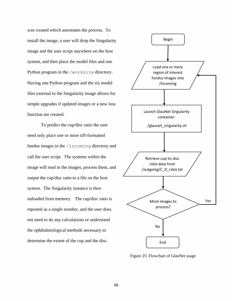
66
was created which automates the process. To
install the image, a user will drop the Singularity
image and the user script anywhere on the host
system, and then place the model files and one
Python program in the /worksite directory.
Having one Python program and the six model
files external to the Singularity image allows for
simple upgrades if updated images or a new loss
function are created.
To predict the cup/disc ratio the user
need only place one or more tiff-formatted
fundus images in the /incoming directory and
call the user script. The systems within the
image will read in the images, process them, and
output the cup/disc ratio to a file on the host
system. The Singularity instance is then
unloaded from memory. The cup/disc ratio is
reported as a single number, and the user does
not need to do any calculations or understand
the ophthalmological methods necessary to
determine the extent of the cup and the disc.
Begin
Load one or more
region of interest
fundus images into
/incoming
Launch GlauNet Singularity
container:
./glaunet_singularity.sh
Retrieve cup-to-disc
ratio data from
/outgoing/C_D_ratio.txt
More images to
process?
End
No
Yes
Figure 25: Flowchart of GlauNet usage

67
6.2. Feasibility of Inexpensive Hardware
The intent of the GlauNet system is to allow users without training as ophthalmologists to
gain one piece of information that points to the likelihood of glaucoma. However, locations
without access to ophthalmologists are likely to also have less access to powerful computers.
The training detailed above in this section created six separate models, each of which was
packaged in a 355 MB H5 file. Files in the H5 format are designed to contain scientific data in a
uniform, readable format, and TensorFlow reads H5 files natively. These H5 files are intended
for distribution with GlauNet, and require no user intervention or understanding; they can be
entirely black boxes to the end user.
To determine the feasibility of running the packaged Singularity image on inexpensive
hardware, an experiment was performed on a CloudLab instance.10 CloudLab is a “facility for
building clouds.” The CloudLab system gives access to bare-metal computers, and gives the
user control over the networking and storage assets a cloud computer has access to. The system
allows control of hardware down to the number of processors and amount of RAM per processor,
allowing an experiment to be both repeatable and precise (CloudLab Team 2020).
A CloudLab instance containing one
core from a single Intel Xeon Silver 4114
processor at 2.20 GHz was instantiated with 4
Gb of RAM. Ubuntu Linux 18.04 and
Singularity version 2.4.2 were installed onto the
instance. Detailed specifications of the instance
hardware and software are given in Table 15.
10 The online interface to CloudLab is available at https://www.cloudlab.us
Operating System Ubuntu Linux 18.04
Containerization Singularity 2.4.2
CPU speed 2,194.910 MHz
CPU cores 1
Cache size 14,080 KB
BOGOMIPS 4,389.82
Memory 4,089 MB
Storage 16,383 MB
Table 15: Test Machine Specifications

68
The six models and the 160x160 pixel region of interest fundus images for all annotators were
uploaded to the instance using SFTP.
A wrapper script was written for the user script (see Section 5.3, above). The wrapper
script outputs a timestamp before and after the user script is run, so it would be possible to
determine how long the CloudLab instance spent loading Singularity, processing the fundus
images through each of the six annotator models, and unloading Singularity. The wrapper script
itself contained nothing between the two timestamp calls other than a call to the user script, and
therefore added negligible time to the process.
Batches of one, two, four, eight,
sixteen, and thirty-two images were
processed through the system. The
images were chosen by randomly
selecting their file numbers without
replacement using a pseudorandom
number generator. Each fundus image
was used as the input to each of the six
models, in turn. Each of the three test
runs for each image count used the same
two, four, etc. images, to minimize
experimental variables.
In an attempt to minimize the effect of a random background process using CPU time and
thereby increasing the time the Singularity container took to do its work, each image count was
processed three separate times, and no user-initiated processes were running on the CloudLab
Figure 26: Mean Time to Process One Image in a
Multi-Image Batch
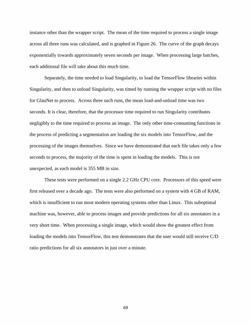
69
instance other than the wrapper script. The mean of the time required to process a single image
across all three runs was calculated, and is graphed in Figure 26. The curve of the graph decays
exponentially towards approximately seven seconds per image. When processing large batches,
each additional file will take about this much time.
Separately, the time needed to load Singularity, to load the TensorFlow libraries within
Singularity, and then to unload Singularity, was timed by running the wrapper script with no files
for GlauNet to process. Across three such runs, the mean load-and-unload time was two
seconds. It is clear, therefore, that the processor time required to run Singularity contributes
negligibly to the time required to process an image. The only other time-consuming functions in
the process of predicting a segmentation are loading the six models into TensorFlow, and the
processing of the images themselves. Since we have demonstrated that each file takes only a few
seconds to process, the majority of the time is spent in loading the models. This is not
unexpected, as each model is 355 MB in size.
These tests were performed on a single 2.2 GHz CPU core. Processors of this speed were
first released over a decade ago. The tests were also performed on a system with 4 GB of RAM,
which is insufficient to run most modern operating systems other than Linux. This suboptimal
machine was, however, able to process images and provide predictions for all six annotators in a
very short time. When processing a single image, which would show the greatest effect from
loading the models into TensorFlow, this test demonstrates that the user would still receive C/D
ratio predictions for all six annotators in just over a minute.

70
7. Conclusion and Further Work
The system described in this thesis, GlauNet, provides a solution for using machine
learning to automatically segment the optic disc and cup from region of interest fundus images,
capture the cup-to-disc ratio from the segmentation, and output six calculated C/D ratios - one
for each of the six annotators in the RIGA dataset. The mean error of GlauNet’s predictions of
pixel labels is 10.3% across all six of the models provided, with a mean precision of 87.7% and a
mean recall of 90.1%. Its pixelwise mean Jaccard Distance from ground truth across all models
is 20.2%.11 The precision of the predicted cup-to-disc ratio across all six models is 0.920, the
recall across all models is 0.946, and the F-measure across all models is 0.933.
For each of the six annotators whose work makes up the RIGA corpus, GlauNet captures
a separate model and outputs a predicted cup-to-disc ratio for that annotator. This separation of
the annotators appears to be unique, even though there is significant interannotator disagreement
as to the segmentation of each fundus image. Other researchers who worked with the RIGA set
have used techniques which either take all annotators together into a single model (Almazroa
IJBI 2018), or combined the annotators’ segmentations together into consensus annotations (Yu
2019).
More work can be done with this system. For instance, a method for importing a fundus
image from a fundus camera would need to be implemented to make GlauNet a turnkey software
appliance. Without access to a fundus camera, this is currently out of reach.
Some further work requires design and coding rather than access to hardware, For
example, while the C/D ratio is a good metric for the development of glaucoma, there are more
metrics which can be captured using a segmentation of the optic cup and disc. GlauNet captures
11 A lower Jaccard Distance is better. 0% Jaccard Distance exactly replicates the ground truth.

71
the horizontal C/D ratio because “studies have shown that the vertical ratio increases faster in
early and intermediate stages of glaucoma,” allowing the disease to be detected earlier in its
progress and heading off blindness with treatment (Tsai 2003). Changes in the morphology of
the retina due to glaucoma can include the vertical C/D ratio being larger than the horizontal C/D
ratio, adding another metric to the detection of the disease (Martus 2005). Specifically, an oval
cup in a round disc can be indicative of glaucoma (Tomlinson 1974). The vertical C/D ratio can
be captured from GlauNet’s segmentations, which will allow the calculation of this new metric.
Notching and irregularities in the rim of the optic disc can be indicative of glaucoma
(Danesh-Meyer 2006, Tsai 2003). A proper segmentation of the optic disc could detect such
irregularities; however, GlauNet does not perfectly convey the border between the optic disc and
the background of the fundus, making it difficult to find such irregularities. More work would
need to be done, to make the models more precise, before such a metric could be captured from
the segmentations.
Taking the opposite tack from identifying irregularities in the border of the segmentation,
it is possible to improve a neural network’s segmentation performance through postprocessing to
reduce the irregularities in region boundaries, fill interior holes, and separate out clusters of
labels with “weak connectivity” (Haidekker 2011). This process might hold some hope for
improvement in the network laid out in this thesis, but the expert annotations which are the
ground truth for this project contain intentional border irregularities, and the “hole” in the center
of each segmentation is a vital piece of information for separating the optic disc from the optic
cup.
Perhaps the most important improvement to the network provided in this thesis would be
to automate the process of localizing the image to a region of interest. The region of interest in a

72
fundus image is the section surrounding the optic disc. For this project, the region of interest
was localized using the human annotators’ segmentations of the image. Almazroa and Burman
have proposed a method of localizing the optic disc by finding the brightest spot in the fundus
image, and centering the localized image there (Almazroa 2017). This localized image could
then be either used as-is, or shown to a human as a sanity check, before being fed into the models
to predict the segmentation of the image.
As the U-Net neural network architecture was used to implement the models, the memory
footprint of the running network is minimized so that it can fit into less than 4 GB of memory
with sufficient space for Linux and Singularity to run comfortably. This minimal footprint is
necessary to fulfill the intentions of the project: a system which can run without issues on
inexpensive hardware and software. The Singularity image is a 1.9 GB file, and therefore has
not been uploaded to a publicly available location. It is, however, available upon request.

73
Works Cited
Almazroa A, S. Alodhayb, E. Osman, et al. “Agreement among ophthalmologists in marking the
optic disc and optic cup in fundus images.” International Ophthalmology: The
International Journal of Clinical Ophthalmology and Visual Sciences. 2016;37(3):701.
doi:10.1007/s10792-016-0329-x.
Almazroa A, W. Sun, S. Alodhayb, K. Raahemifar, V. Lakshminarayanan. “Optic disc
segmentation for glaucoma screening system using fundus images.” Clin Ophthalmol.
2017;11:2017-2029 https://doi.org/10.2147/OPTH.S140061
Almazroa A, W. Sun, S. Alodhayb, K. Raahemifar, V. Lakshminarayanan. “An Automatic
Image Processing System for Glaucoma Screening.” International Journal of Biomedical
Imaging. 2017;11:2017-2029 https://doi.org/10.1155/2017/4826385
Almazroa, Ahmed, Sami Alodhayb, Essameldin Osman, Eslam Ramadan, Mohammed
Hummadi, Mohammed Dlaim, Muhannad Alkatee, Kaamran Raahemifar, Vasudevan
Lakshminarayanan, “Retinal fundus images for glaucoma analysis: the RIGA dataset.”
Proc. SPIE 10579, Medical Imaging 2018: Imaging Informatics for Healthcare, Research,
and Applications, 105790B (6 March 2018); doi: 10.1117/12.2293584;
https://doi.org/10.1117/12.2293584
Almazroa, A. (2018). “Retinal fundus images for glaucoma analysis: the RIGA dataset [Data
set]”. University of Michigan - Deep Blue. https://doi.org/10.7302/Z23R0R29
Alto, Valentina. “Neural Networks: parameters, hyperparameters and optimization strategies.”
Towards Data Science. July 5, 2019. https://towardsdatascience.com/neural-networks-
parameters-hyperparameters-and-optimization-strategies-3f0842fac0a5
Amazon. “Amazon EC2 Pricing.” Web. 2020. https://aws.amazon.com/ec2/pricing/on-demand/

74
Aquino, Arturo, Manuel Emilio Gegúndez-Arias, and Diego Marín. “Detecting the optic disc
boundary in digital fundus images using morphological, edge detection, and feature
extraction techniques.” IEEE Transactions on Medical Imaging. 2010; 29(10) 1860-
1869
Armaly MF. Genetic Determination of Cup/Disc: Ratio of the Optic Nerve. Arch Ophthalmol.
1967;78(1):35–43. doi:10.1001/archopht.1967.00980030037007
Arnekvist, Isac, J. Frederico Carvalho, Danica Kragic, and Johannes A. Stork. 2020. “The Effect
of Target Normalization and Momentum on Dying ReLU.”
https://search.ebscohost.com/login.aspx?direct=true&AuthType=sso&db=edsarx&AN=e
dsarx.2005.06195&site=eds-live&scope=site.
Bertels, Jeroen, Tom Eelbode, Maxim Berman, Dirk Vandermeulen, Frederik Maes, Raf
Bisschops, and Matthew Blaschko. 2019. “Optimizing the Dice Score and Jaccard Index
for Medical Image Segmentation: Theory & Practice.” doi:10.1007/978-3-030-32245-
8_11.
Blanford, Richard. “Beware the hidden costs of cloud computing.” 2018. IT Pro Portal.
https://www.itproportal.com/features/beware-the-hidden-costs-of-cloud-computing/
Buda, Mateusz, Atsuto Maki, and Maciej A Mazurowski. “A Systematic Study of the Class
Imbalance Problem in Convolutional Neural Networks.” Neural Networks 106 (2018):
249-59.
Budenz, Donald L, Keith Barton, Julia Whiteside-de Vos, Joyce Schiffman, Jagadeesh Bandi,
Winifred Nolan, Leon Herndon, Hanna Kim, Graham Hay-Smith, and James M Tielsch.
“Prevalence of Glaucoma in an Urban West African Population: The Tema Eye Survey.”
JAMA Ophthalmology 131.5 (2013): 651-58.

75
Chakravarty, Arunava, and Jayanthi Sivaswamy. 2017. “Joint Optic Disc and Cup Boundary
Extraction from Monocular Fundus Images.” Computer Methods & Programs in
Biomedicine 147 (August): 51–61. doi:10.1016/j.cmpb.2017.06.004.
CloudLab Team, The. “The CloudLab Manual.” 2020. http://docs.cloudlab.us/cloudlab-
manual.html
Danesh-Meyer, H V, B J Gaskin, T. Jayusundera, M. Donaldson, and G D Gamble. “Comparison
of Disc Damage Likelihood Scale, Cup to Disc Ratio, and Heidelberg Retina Tomograph
in the Diagnosis of Glaucoma.” British Journal of Ophthalmology 90.4 (2006): 437-41.
Duplyakin, Dmitry, Robert Ricci, Aleksander Maricq, Gary Wong, Jonathon Duerig, Eric Eide,
Leigh Stoller, Mike Hibler, David Johnson, Kirk Webb, Aditya Akella, Kuangching
Wang, Glenn Ricart, Larry Landweber, Chip Elliott, Michael Zink, Emmanuel Cecchet,
Snigdhaswin Kar, and Prabodh Mishra. 2019. “Design and Operation of Cloudlab.”
Proceedings of the USENIX Annual Technical Conference (ATC). pp 1-14.
Dwivedi, Priya “Understanding and Coding a ResNet in Keras.” 2019. Web.
https://towardsdatascience.com/understanding-and-coding-a-resnet-in-keras-
446d7ff84d33
Edward, Deepak P., and Thasarat S. Vajaranant. Glaucoma. Oxford: Oxford UP, 2013. Oxford
American Ophthalmology Library.
Escobar, Angela. "How Much Does Telemedicine Software Cost?" KompareIt. 2020. Web.
https://www.kompareit.com/business/medical-telemedicine-how-much-cost.html
Fanelli, James L. “Same Cup, Different Ratios.” Review of Optometry 150 (10): 90–93 (2013).
76
Forchheimer, De Moraes, Teng, Folgar, Tello, Ritch, and Liebmann. “Baseline Mean Deviation
and Rates of Visual Field Change in Treated Glaucoma Patients.” Eye 25.5 (2011): 626-
32.
Foster, Paul J, Ralf Buhrmann, Harry A Quigley, and Gordon J Johnson. “The Definition and
Classification of Glaucoma in Prevalence Surveys.” British Journal of Ophthalmology
86.2 (2002): 238-23842.
Ganesh Babu, T.R., S. Shenbaga Devi, and Rengaraj Venkatesh. “Automatic Detection of
Glaucoma Using Optical Coherence Tomography Image.” Journal of Applied Sciences
12 (20): 2128-2138, 2012.
Ganesh Babu, T R, S Shenbaga Devi, and R Venkatesh. 2015. “Optic Nerve Head Segmentation
Using Fundus Images and Optical Coherence Tomography Images for Glaucoma
Detection.” Biomedical Papers of the Medical Faculty of the University Palacky,
Olomouc, Czechoslovakia 159 (4): 607–15. doi:10.5507/bp.2015.053.
Google. “Classification: ROC Curve and AUC.” (2020) Web.
https://developers.google.com/machine-learning/crash-course/classification/roc-and-auc
Haidekker, Mark. Advanced Biomedical Image Analysis. 2011. John Wiley & Sons.
Hao, Zhixu. “Implementation of deep learning framework – Unet, using Keras.” 2018. Web.
https://github.com/zhixuhao/unet
Hao, Ziqiang, Guangxu Wan, Victor Oluwaferanmi Adewuyi, and Weida Zhan. 2020.
“Improved Faster R-CNN for Detecting Small Objects and Occluded Objects in Electron
Microscope Imaging.” Acta Microscopica 29 (1): 542–51.

77
Hayamizu F, Yamazaki Y, Nakagami T, and Mizuki K. “Optic Disc Size and Progression of
Visual Field Damage in Patients with Normal-tension Glaucoma.” Clinical
Ophthalmology (2013): 807-13.
He, Kaiming, Xiangyu Zhang, Shaoqing Ren, and Jian Sun. “Delving Deep into Rectifiers:
Surpassing Human-Level Performance on ImageNet Classification.” 2015 IEEE
International Conference on Computer Vision (ICCV), January 2015, 1026.
Hsieh Jui-chien, and Hsu Meng-Wei. 2012. “A Cloud Computing Based 12-Lead ECG
Telemedicine Service.” BMC Medical Informatics and Decision Making 12 (1): 77.
doi:10.1186/1472-6947-12-77.
Owen Jones, Robert Maillardet, and Andrew Robinson. Introduction to Scientific Programming
and Simulation Using R, Second Edition. CRC Press: Parkville, Australia; 2014.
Rezaul, Karim and Pradeep Pujari. Practical Convolutional Neural Networks. Packt Publishing;
2018.
Kayalibay, Baris, Grady Jensen, and Patrick van der Smagt. 2017. “CNN-Based Segmentation of
Medical Imaging Data.”
https://search.ebscohost.com/login.aspx?direct=true&AuthType=sso&db=edsarx&AN=e
dsarx.1701.03056&site=eds-live&scope=site.
Kessing, Svend Vedel., and John Thygesen. Primary Angle-closure and Angle-closure
Glaucoma. Hague, Netherlands : Gilsum, NH: Kugler ; Pathway Book Service, 2007.
Khalil. T., M. U. Akram, H. Raja, A. Jameel and I. Basit, “Detection of Glaucoma Using Cup to
Disc Ratio From Spectral Domain Optical Coherence Tomography Images,” IEEE
Access, vol. 6, pp. 4560-4576, 2018, doi: 10.1109/ACCESS.2018.2791427.
78
Kolb, H. “Facts and Figures Concerning the Human Retina.” National Center for Biotechnical
Information at the U.S. National Library of Medicine. 2017.
https://www.ncbi.nlm.nih.gov/books/NBK11556/
Kooner, Karanjit S., and Thom J. Zimmerman. Clinical Pathways in Glaucoma. New York:
Thieme, 2001.
Kurtzer GM, V. Sochat, MW Bauer. 2017 “Singularity: Scientific containers for mobility of
compute.” PLoS ONE 12(5): e0177459. https://doi.org/10.1371/journal.pone.0177459
Li, F., Ranjay Krishna, Danfei Xu, and Amelie Byun. “CS231n: Convolutional Neural Networks
for Visual Recognition.” (2020) Stanford University. Web. http://cs231n.stanford.edu/
Liu, J., D. W. K. Wong, J. H. Lim, H. Li, N. M. Tan, and T. Y. Wong. 2009. “ARGALI: An
Automatic Cup-to-Disc Ratio Measurement System for Glaucoma Detection and
AnaLysIs Framework.” Proceedings of SPIE, no. 1 (November): 72603K.
Lu, Lu, Yeonjong Shin, Yanhui Su, and George Em Karniadakis. 2019. “Dying ReLU and
Initialization: Theory and Numerical Examples.”
https://search.ebscohost.com/login.aspx?direct=true&AuthType=sso&db=edsarx&AN=e
dsarx.1903.06733&site=eds-live&scope=site.
Martus, Peter, Andrea Stroux, Wido Budde, Christian Mardin, Matthias Korth, and Jost Jonas.
“Predictive Factors for Progressive Optic Nerve Damage in Various Types of Chronic
Open-angle Glaucoma.” American Journal of Ophthalmology 139.6 (2005): 999-1009
Medici Technologies. “Pricing.” 2020. Web. https://www.medici.md/doctors/pricing
Mishkin, Dmytro, and Jiri Matas. “All You Need Is a Good Init,” 2016. International
Conference on Learning Representations.

79
Moraru, Aurelian. 2017. “The New Telemedicine Business Model.” Benchmarking
Telemedicine: Improving Health Security in the Balkans. NATO Science for Peace and
Security Series-D: Information and Communication Security: Volume 49. IOS Press.
Riccardo Miotto, Matteo Danieletto, Jerome R. Scelza, Brian A. Kidd, and Joel T. Dudley. 2018.
“Reflecting Health: Smart Mirrors for Personalized Medicine.” Npj Digital Medicine 1
(1): 1–7. doi:10.1038/s41746-018-0068-7.
Mohammadi, S-Farzad, Sara Mirhadi, Hadi Mehrjardi, Akbar Fotouhi, Sahar Vakili, Mercede
Majdi, and Sasan Moghimi. “An Algorithm for Glaucoma Screening in Clinical Settings
and Its Preliminary Performance Profile.” Journal of Ophthalmic & Vision Research 8.4
(2013): 314-20.
Nithya, R. and N. Venkateswaran. (2015). “Analysis of Segmentation Algorithms in Colour
Fundus and OCT Images for Glaucoma Detection.” Indian Journal of Science and
Technology, 8.
Okimoto S, K. Yamashita, T. Shibata, Y. Kiuchi. 2015. “Morphological Features and Important
Parameters of Large Optic Discs for Diagnosing Glaucoma.” PLoS ONE 10(3):
e0118920.doi:10.1371/journal.pone.0118920
Ontañón, Santiago. “An Overview of Distance and Similarity Functions for Structured Data.”
Artificial Intelligence Review: An International Science and Engineering Journal, 2020,
1. doi:10.1007/s10462-020-09821-w.
Ronneberger, Olaf, Philipp Fischer, and Thomas Brox. 2015. “U-Net: Convolutional Networks
for Biomedical Image Segmentation.”
https://search.ebscohost.com/login.aspx?direct=true&AuthType=sso&db=edsarx&AN=e
dsarx.1505.04597&site=eds-live&scope=site.
80
Rumelhart, David E., Geoffrey E. Hinton, and Ronald J. Williams. 1986. “Learning
Representations by Back-Propagating Errors.” Nature 323 (6088): 533–36.
Shringarpure, Suyash, Andrew Carroll, Francisco M De La Vega, and Carlos D Bustamante.
2015. “Inexpensive and Highly Reproducible Cloud-Based Variant Calling of 2,535
Human Genomes.” PLoS ONE 10 (6): e0129277. doi:10.1371/journal.pone.0129277.
Sommer, A., J M Tielsch, J. Katz, H A Quigley, J D Gottsch, J C Javitt, J F Martone, R M
Royall, K A Witt, and S. Ezrine. “Racial Differences in the Cause-specific Prevalence of
Blindness in East Baltimore.” The New England Journal of Medicine 325.20 (1991):
1412-1417.
Song, T., F. Meng, A. Rodriguez-Paton, P. Li, P. Zheng, and X. Wang. 2019. “U-Next: A Novel
Convolution Neural Network With an Aggregation U-Net Architecture for Gallstone
Segmentation in CT Images.” IEEE Access 7 (January): 166823–32.
doi:10.1109/ACCESS.2019.2953934.
TensorFlow Team. “TensorFlow Core v2.2.0.” 2020. https://www.tensorflow.org/api_docs.
Thada, Vikas, and Vivek Jaglan. “Comparison of Jaccard, Dice, Cosine Similarity Coefficient to
Find Best Fitness Value for Web Retrieved Documents Using Genetic Algorithm.”
International Journal of Innovations in Engineering and Technology 2, no. 4 (2013):
202-205.
Tomlinson, Alan and Calbert Phillips. “Ovalness of the optic cup and disc in the normal eye.”
British Journal of Ophthalmology. 1974. 10.1136/bjo.58.5.543.
Tsai, C. “How to Evaluate the Suspicious Optic Disc.” Review of Ophthalmology, MD, New
York City, Jun. 2005

81
Tsai, James C and Max Forbes. Medical Management of Glaucoma. Professional
Communication Inc, Oklahoma; 2003. 240 Pages ISBN 1-884735-80-0 Media
Type:textbook.
Wang, Ya X., Xu, Liang, Lu, Wen, Liu, Feng J., Qu, Yuan Z., Wang, Jian, and Jonas, Jost B.
“Parapapillary Atrophy in Patients with Intracranial Tumours.” Acta Ophthalmologica
91.6 (2013): 521-25.
Wu, Menglin, Theodore Leng, Luis de Sisternes, Daniel L Rubin, and Qiang Chen. 2015.
“Automated Segmentation of Optic Disc in SD-OCT Images and Cup-to-Disc Ratios
Quantification by Patch Searching-Based Neural Canal Opening Detection.” Optics
Express 23 (24): 31216–29. doi:10.1364/OE.23.031216.
Yu, Shuang, Di Xiao, Shaun Frost, and Yogesan Kanagasingam. 2019. “Robust Optic Disc and
Cup Segmentation with Deep Learning for Glaucoma Detection.” Computerized Medical
Imaging and Graphics 74 (June): 61–71. doi:10.1016/j.compmedimag.2019.02.005.
This project would not have been possible without the annotations provided in the RIGA dataset,
which were created by the MESSIDOR program, and the Magrabi Eye Center and Bin
Rushed Ophthalmic Center in Saudi Arabia.