a logic for reasoning about evidence - cornell … the observations above suggest that if we attempt...
TRANSCRIPT
Journal of Artificial Intelligence Research 25 (2006) ?–? Submitted 11/05; published 04/06
A Logic for Reasoning about Evidence
Joseph Y. Halpern [email protected] University, Ithaca, NY 14853 USA
Riccardo Pucella [email protected]
Northeastern University, Boston, MA 02115 USA
Abstract
We introduce a logic for reasoning about evidence that essentially views evidence asa function from prior beliefs (before making an observation) to posterior beliefs (aftermaking the observation). We provide a sound and complete axiomatization for the logic,and consider the complexity of the decision problem. Although the reasoning in the logicis mainly propositional, we allow variables representing numbers and quantification overthem. This expressive power seems necessary to capture important properties of evidence.
1. Introduction
Consider the following situation, essentially taken from Halpern and Tuttle (1993) andFagin and Halpern (1994). A coin is tossed, which is either fair or double-headed. The coinlands heads. How likely is it that the coin is double-headed? What if the coin is tossed20 times and it lands heads each time? Intuitively, it is much more likely that the coinis double-headed in the latter case than in the former. But how should the likelihood bemeasured? We cannot simply compute the probability of the coin being double-headed;assigning a probability to that event requires that we have a prior probability on the coinbeing double-headed. For example, if the coin was chosen at random from a barrel withone billion fair coins and one double-headed coin, it is still overwhelmingly likely that thecoin is fair, and that the sequence of 20 heads is just unlucky. However, in the problemstatement, the prior probability is not given. We can show than any given prior probabilityon the coin being double-headed increases significantly as a result of seeing 20 heads. But,intuitively, it seems that we should be able to say that seeing 20 heads in a row providesa great deal of evidence in favor of the coin being double-headed without invoking a prior.There has been a great deal of work in trying to make this intuition precise, which we nowreview.
The main feature of the coin example is that it involves a combination of probabilis-tic outcomes (e.g., the coin tosses) and nonprobabilistic outcomes (e.g., the choice of thecoin). There has been a great deal of work on reasoning about systems that combine bothprobabilistic and nondeterministic choices; see, for example, Vardi (1985), Fischer and Zuck(1988), Halpern, Moses, and Tuttle (1988), Halpern and Tuttle (1993), de Alfaro (1998),He, Seidel, and McIver (1997). However, the observations above suggest that if we attemptto formally analyze this situation in one of those frameworks, which essentially permit onlythe modeling of probabilities, we will not be able to directly capture this intuition aboutincreasing likelihood. To see how this plays out, consider a formal analysis of the situationin the Halpern-Tuttle (1993) framework. Suppose that Alice nonprobabilistically chooses
c©2006 AI Access Foundation. All rights reserved.

Halpern & Pucella
one of two coins: a fair coin with probability 1/2 of landing heads, or a double-headed coinwith probability 1 of landing heads. Alice tosses this coin repeatedly. Let ϕk be a formulastating: “the kth coin toss lands heads”. What is the probability of ϕk according to Bob,who does not know which coin Alice chose, or even the probability of Alice’s choice?
According to the Halpern-Tuttle framework, this can be modeled by considering theset of runs describing the states of the system at each point in time, and partitioningthis set into two subsets, one for each coin used. In the set of runs where the fair coinis used, the probability of ϕk is 1/2; in the set of runs where the double-headed coin isused, the probability of ϕk is 1. In this setting, the only conclusion that can be drawn is(PrB(ϕk) = 1/2) ∨ (PrB(ϕk) = 1). (This is of course the probability from Bob’s point ofview; Alice presumably knows which coin she is using.) Intuitively, this seems reasonable:if the fair coin is chosen, the probability that the kth coin toss lands heads, according toBob, is 1/2; if the double-headed coin is chosen, the probability is 1. Since Bob does notknow which of the coins is being used, that is all that can be said.
But now suppose that, before the 101st coin toss, Bob learns the result of the first 100tosses. Suppose, moreover, that all of these landed heads. What is the probability that the101st coin toss lands heads? By the same analysis, it is still either 1/2 or 1, depending onwhich coin is used.
This is hardly useful. To make matters worse, no matter how many coin tosses Bobwitnesses, the probability that the next toss lands heads remains unchanged. But thisanswer misses out on some important information. The fact that all of the first 100 cointosses are heads is very strong evidence that the coin is in fact double-headed. Indeed, astraightforward computation using Bayes’ Rule shows that if the prior probability of thecoin being double-headed is α, then after observing that all of the 100 tosses land heads,the probability of the coin being double-headed becomes
α
α+ 2−100(1− α)=
2100α
2100α+ (1− α).
However, note that it is not possible to determine the posterior probability that the coin isdouble-headed (or that the 101st coin toss is heads) without the prior probability α. Afterall, if Alice chooses the double-headed coin with probability only 10−100, then it is stilloverwhelmingly likely that the coin used is in fact fair, and that Bob was just very unluckyto see such an unrepresentative sequence of coin tosses.
None of the frameworks described above for reasoning about nondeterminism and prob-ability takes the issue of evidence into account. On the other hand, evidence has beendiscussed extensively in the philosophical literature. Much of this discussion occurs in thephilosophy of science, specifically confirmation theory, where the concern has been histori-cally to assess the support that evidence obtained through experimentation lends to variousscientific theories (Carnap, 1962; Popper, 1959; Good, 1950; Milne, 1996). (Kyburg (1983)provides a good overview of the literature.)
In this paper, we introduce a logic for reasoning about evidence. Our logic extends alogic defined by Fagin, Halpern and Megiddo (1990) (FHM from now on) for reasoning aboutlikelihood expressed as either probability or belief. The logic has first-order quantificationover the reals (so includes the theory of real closed fields), as does the FHM logic, forreasons that will shortly become clear. We add observations to the states, and provide an
2
A Logic for Reasoning about Evidence
additional operator to talk about the evidence provided by particular observations. We alsorefine the language to talk about both the prior probability of hypotheses and the posteriorprobability of hypotheses, taking into account the observation at the states. This lets uswrite formulas that talk about the relationship between the prior probabilities, the posteriorprobabilities, and the evidence provided by the observations.
We then provide a sound and complete axiomatization for the logic. To obtain such anaxiomatization, we seem to need first-order quantification in a fundamental way. Roughlyspeaking, this is because ensuring that the evidence operator has the appropriate propertiesrequires us to assert the existence of suitable probability measures. It does not seem possi-ble to do this without existential quantification. Finally, we consider the complexity of thesatisfiability problem. The complexity problem for the full language requires exponentialspace, since it incorporates the theory of real closed fields, for which an exponential-spacelower bound is known (Ben-Or, Kozen, & Reif, 1986). However, we show that the satisfia-bility problem for a propositional fragment of the language, which is still strong enough toallow us to express many properties of interest, is decidable in polynomial space.
It is reasonable to ask at this point why we should bother with a logic of evidence. Ourclaim is that many decisions in practical applications are made on the basis of evidence.To take an example from security, consider an enforcement mechanism used to detect andreact to intrusions in a computer system. Such an enforcement mechanism analyzes thebehavior of users and attempts to recognize intruders. Clearly the mechanism wants tomake sensible decisions based on observations of user behaviors. How should it do this?One way is to think of an enforcement mechanism as accumulating evidence for or againstthe hypothesis that the user is an intruder. The accumulated evidence can then be used asthe basis for a decision to quarantine a user. In this context, it is not clear that there is areasonable way to assign a prior probability on whether a user is an intruder. If we wantto specify the behavior of such systems and prove that they meet their specifications, it ishelpful to have a logic that allows us to do this. We believe that the logic we propose hereis the first to do so.
The rest of the paper is organized as follows. In the next section, we formalize a notionof evidence that captures the intuitions outlined above. In Section 3, we introduce our logicfor reasoning about evidence. In Section 4, we present an axiomatization for the logic andshow that it is sound and complete with respect to the intended models. In Section 5, wediscuss the complexity of the decision problem of our logic. In Section 6, we examine somealternatives to the definition of weight of evidence we use. For ease of exposition, in mostof the paper, we consider a system where there are only two time points: before and afterthe observation. In Section 7, we extend our work to dynamic systems, where there can bemultiple pieces of evidence, obtained at different points in time. The proofs of our technicalresults can be found in the appendix.
2. Measures of Confirmation and Evidence
In order to develop a logic for reasoning about evidence, we need to first formalize anappropriate notion of evidence. In this section, we review various formalizations from theliterature, and discuss the formalization we use. Evidence has been studied in depth in thephilosophical literature, under the name of confirmation theory. Confirmation theory aims
3
Halpern & Pucella
at determining and measuring the support a piece of evidence provides an hypothesis. As wementioned in the introduction, many different measures of confirmation have been proposedin the literature. Typically, a proposal has been judged on the degree to which it satisfiesvarious properties that are considered appropriate for confirmation. For example, it may berequired that a piece of evidence e confirms an hypothesis h if and only if e makes h moreprobable. We have no desire to enter the debate as to which class of measures of confirmationis more appropriate. For our purposes, most confirmation functions are inappropriate:they assume that we are given a prior on the set of hypotheses and observations. Bymarginalization, we also have a prior on hypotheses, which is exactly the information we donot have and do not want to assume. One exception is measures of evidence that use thelog-likelihood ratio. In this case, rather than having a prior on hypotheses and observations,it suffices that there be a probability µh on observations for each hypothesis h: intuitively,µh(ob) is the probability of observing ob when h holds. Given an observation ob, the degreeof confirmation that it provides for an hypothesis h is
l(ob, h) = log(µh(ob)µh(ob)
),
where h represents the hypothesis other than h (recall that this approach applies only ifthere are two hypotheses). Thus, the degree of confirmation is the ratio between thesetwo probabilities. The use of the logarithm is not critical here. Using it ensures that thelikelihood is positive if and only if the observation confirms the hypothesis. This approachhas been advocated by Good (1950, 1960), among others.1
One problem with the log-likelihood ratio measure l as we have defined it is that it canbe used only to reason about evidence discriminating between two competing hypotheses,namely between an hypothesis h holding and the hypothesis h not holding. We would likea measure of confirmation along the lines of the log-likelihood ratio measure, but that canhandle multiple competing hypotheses. There have been a number of such generalizations,for example, by Pearl (1988) and Chan and Darwiche (2005). We focus here on the gener-alization given by Shafer (1982) in the context of the Dempster-Shafer theory of evidencebased on belief functions (Shafer, 1976); it was further studied by Walley (1987). Thedescription here is taken mostly from Halpern and Fagin (1992). While this measure ofconfirmation has a number of nice properties of which we take advantage, much of the workpresented in this paper can be adapted to different measures of confirmation.
We start with a finite set H of mutually exclusive and exhaustive hypotheses; thus,exactly one hypothesis holds at any given time. Let O be the set of possible observations(or pieces of evidence). For simplicity, we assume that O is finite. Just as in the case of log-likelihood, we also assume that, for each hypotheses h ∈ H, there is a probability measureµh on O such that µh(ob) is the probability of ob if hypothesis h holds. Furthermore, weassume that the observations in O are relevant to the hypotheses: for every observationob ∈ O, there must be an hypothesis h such that µh(ob) > 0. (The measures µh are oftencalled likelihood functions in the literature.) We define an evidence space (over H and O)
1. Another related approach, the Bayes factor approach, is based on taking the ratio of odds rather thanlikelihoods (Good, 1950; Jeffrey, 1992). We remark that in the literature, confirmation is usually takenwith respect to some background knowledge. For ease of exposition, we ignore background knowledgehere, although it can easily be incorporated into the framework we present.
4
A Logic for Reasoning about Evidence
to be a tuple E = (H,O,µ), where µ is a function that assigns to every hypothesis h ∈ Hthe likelihood function µ(h) = µh. (For simplicity, we usually write µh for µ(h), when thethe function µ is clear from context.)
Given an evidence space E , we define the weight that the observation ob lends to hy-pothesis h, written wE(ob, h), as
wE(ob, h) =µh(ob)∑
h′∈H µh′(ob). (1)
The measure wE always lies between 0 and 1; intuitively, if wE(ob, h) = 1, then ob fullyconfirms h (i.e., h is certainly true if ob is observed), while if wE(ob, h) = 0, then obdisconfirms h (i.e., h is certainly false if ob is observed). Moreover, for each fixed observationob for which
∑h∈H µh(ob) > 0,
∑h∈HwE(ob, h) = 1, and thus the weight of evidence
wE looks like a probability measure for each ob. While this has some useful technicalconsequences, one should not interpret wE as a probability measure. Roughly speaking, theweight wE(ob, h) is the likelihood that h is the right hypothesis in the light of observationob.2 The advantages of wE over other known measures of confirmation are that (a) it isapplicable when we are not given a prior probability distribution on the hypotheses, (b) itis applicable when there are more than two competing hypotheses, and (c) it has a fairlyintuitive probabilistic interpretation.
An important problem in statistical inference (Casella & Berger, 2001) is that of choosingthe best parameter (i.e., hypothesis) that explains observed data. When there is no prioron the parameters, the “best” parameter is typically taken to be the one that maximizesthe likelihood of the data given that parameter. Since wE is just a normalized likelihoodfunction, the parameter that maximizes the likelihood will also maximize wE . Thus, if allwe are interested in is maximizing likelihood, there is no need to normalize the evidence aswe do. We return to the issue of normalization in Section 6.3
Note that if H = {h1, h2}, then wE in some sense generalizes the log-likelihood ratiomeasure. More precisely, for a fixed observation ob, wE(ob, ·) induces the same relative orderon hypotheses as l(ob, ·), and for a fixed hypothesis h, wE(·, h) induces the same relativeorder on observations as l(·, h).
Proposition 2.1: For all ob, we have wE(ob, hi) ≥ wE(ob, h3−i) if and only if l(ob, hi) ≥l(ob, h3−i), for i = 1, 2, and for all h, ob, and ob ′, we have wE(ob, h) ≥ wE(ob ′, h) if andonly if l(ob, h) ≥ l(ob ′, h).
2. We could have taken the log of the ratio to make wE parallel the log-likelihood ratio l defined earlier,but there are technical advantages in having the weight of evidence be a number between 0 and 1.
3. Another representation of evidence that has similar characteristics to wE is Shafer’s original representa-tion of evidence via belief functions (Shafer, 1976), defined as
wSE (ob, h) =
µh(ob)
maxh∈H µh(ob).
This measure is known in statistical hypothesis testing as the generalized likelihood-ratio statistic. It isanother generalization of the log-likelihood ratio measure l. The main difference between wE and wS
E ishow they behave when one considers the combination of evidence, which we discuss later in this section.As Walley (1987) and Halpern and Fagin (1992) point out, wE gives more intuitive results in this case.We remark that the parameter (hypothesis) that maximized likelihood also maximizes wS
E , so wSE can
also be used in statistical inference.
5

Halpern & Pucella
Although wE(ob, ·) behaves like a probability measure on hypotheses for every observa-tion ob, one should not think of it as a probability; the weight of evidence of a combinedhypothesis, for instance, is not generally the sum of the weights of the individual hypothe-ses (Halpern & Pucella, 2005a). Rather, wE(ob, ·) is an encoding of evidence. But whatis evidence? Halpern and Fagin (1992) have suggested that evidence can be thought of asa function mapping a prior probability on the hypotheses to a posterior probability, basedon the observation made. There is a precise sense in which wE can be viewed as a functionthat maps a prior probability µ0 on the hypotheses H to a posterior probability µob basedon observing ob, by applying Dempster’s Rule of Combination (Shafer, 1976). That is,
µob = µ0 ⊕ wE(ob, ·), (2)
where ⊕ combines two probability distributions on H to get a new probability distributionon H defined as follows:
(µ1 ⊕ µ2)(H) =∑
h∈H µ1(h)µ2(h)∑h∈H µ1(h)µ2(h)
.
(Dempster’s Rule of Combination is used to combine belief functions. The definition of ⊕ ismore complicated when considering arbitrary belief functions, but in the special case wherethe belief functions are in fact probability measures, it takes the form we give here.)
Bayes’ Rule is the standard way of updating a prior probability based on an observation,but it is only applicable when we have a joint probability distribution on both the hypothesesand the observations (or, equivalently, a prior on hypotheses together with the likelihoodfunctions µh for h ∈ H), something which we do not want to assume we are given. Inparticular, while we are willing to assume that we are given the likelihood functions, weare not willing to assume that we are given a prior on hypotheses. Dempster’s Rule ofCombination essentially “simulates” the effects of Bayes’ Rule. The relationship betweenDempster’s Rule and Bayes’ Rule is made precise by the following well-known theorem.
Proposition 2.2: (Halpern & Fagin, 1992) Let E = (H,O,µ) be an evidence space.Suppose that P is a probability on H × O such that P (H × {ob} | {h} × O) = µh(ob)for all h ∈ H and all ob ∈ O. Let µ0 be the probability on H induced by marginal-izing P ; that is, µ0(h) = P ({h} × O). For ob ∈ O, let µob = µ0 ⊕ wE(ob, ·). Thenµob(h) = P ({h} × O | H × {ob}).
In other words, when we do have a joint probability on the hypotheses and observa-tions, then Dempster’s Rule of Combination gives us the same result as a straightforwardapplication of Bayes’ Rule.
Example 2.3: To get a feel for how this measure of evidence can be used, consider avariation of the two-coins example in the introduction. Assume that the coin chosen byAlice is either double-headed or fair, and consider sequences of a hundred tosses of that coin.Let O = {m : 0 ≤ m ≤ 100} (the number of heads observed), and let H = {F,D}, where Fis “the coin is fair”, and D is “the coin is double-headed”. The probability spaces associatedwith the hypotheses are generated by the following probabilities for simple observations m:
µF (m) =1
2100
(100m
)µD(m) =
{1 if m = 1000 otherwise.
6

A Logic for Reasoning about Evidence
(We extend by additivity to the whole set O.) Take E = (H,O,µ), where µ(F ) = µF andµ(D) = µD. For any observation m 6= 100, the weight in favor of F is given by
wE(m,F ) =1
2100
(100m
)0 + 1
2100
(100m
) = 1,
which means that the support of m is unconditionally provided to F ; indeed, any suchsequence of tosses cannot appear with the double-headed coin. Thus, if m 6= 100, we getthat
wE(m,D) =0
0 + 12100
(100m
) = 0.
What happens when the hundred coin tosses are all heads? It is straightforward to checkthat
wE(100, F ) =1
2100
1 + 12100
=1
1 + 2100wE(100, D) =
11 + 1
2100
=2100
1 + 2100;
this time there is overwhelmingly more evidence in favor of D than F .Note that we have not assumed any prior probability. Thus, we cannot talk about the
probability that the coin is fair or double-headed. What we have is a quantitative assessmentof the evidence in favor of one of the hypotheses. However, if we assume a prior probabilityα on the coin being fair and m heads are observed after 100 tosses, then the probabilitythat the coin is fair is 1 if m 6= 100; if m = 100 then, applying the rule of combination, theposterior probability of the coin being fair is α/(α+ (1− α)2100). ut
Can we characterize weight functions using a small number of properties? More precisely,given sets H and O, and a function f from O ×H to [0, 1], are there properties of f thatensure that there are likelihood functions µ such that f = wE for E = (H,O,µ)? Aswe saw earlier, for a fixed observation ob, f essentially acts like a probability measure onH. However, this is not sufficient to guarantee that f is a weight function. Consider thefollowing example, with O = {ob1, ob2} and H = {h1, h2, h3}:
f(ob1, h1) = 1/4 f(ob2, h1) = 1/4f(ob1, h2) = 1/4 f(ob2, h2) = 1/2f(ob1, h3) = 1/2 f(ob2, h3) = 1/4.
It is straightforward to check that f(ob1, ·) and f(ob2, ·) are probability measures on H,but that there is no evidence space E = (H,O,µ) such that f = wE . Indeed, assume thatwe do have such µh1 , µh2 , µh3 . By the definition of weight of evidence, and the fact that fis that weight of evidence, we get the following system of equations:
µh1(ob1)
µh1(ob1)+µh2
(ob1)+µh3(ob1) = 1/4
µh2(ob1)
µh1(ob1)+µh2
(ob1)+µh3(ob1) = 1/4
µh3(ob1)
µh1(ob1)+µh2
(ob1)+µh3(ob1) = 1/2
µh1(ob2)
µh1(ob2)+µh2
(ob2)+µh3(ob2) = 1/4
µh2(ob2)
µh1(ob2)+µh2
(ob2)+µh3(ob2) = 1/2
µh3(ob2)
µh1(ob2)+µh2
(ob2)+µh3(ob2) = 1/4.
It is now immediate that there exist α1 and α2 such that µhi(obj) = αjf(obj , hi), for
i = 1, 2, 3. Indeed, αj = µh1(obj) + µh2(obj) + µh3(obj), for j = 1, 2. Moreover, since µhiis
a probability measure, we must have that
µhi(ob1) + µhi
(ob2) = α1f(ob1, hi) + α2f(ob2, hi) = 1,
7

Halpern & Pucella
for i = 1, 2, 3. Thus,
α1/4 + α2/4 = α1/4 + α2/2 = α1/2 + α4/4 = 1.
These constraints are easily seen to be unsatisfiable.This argument generalizes to arbitrary functions f ; thus, a necessary condition for f to
be a weight function is that there exists αi for each observation obi such that µh(obi) =αif(obi, h) for each hypothesis h is a probability measure, that is, α1f(ob1, h) + · · · +αkf(obk, h) = 1. In fact, when combined with the constraint that f(ob, ·) is a probabilitymeasure for a fixed ob, this condition turns out to be sufficient, as the following theoremestablishes.
Theorem 2.4: Let H = {h1, . . . , hm} and O = {ob1, . . . , obn}, and let f be a real-valuedfunction with domain O×H such that f(ob, h) ∈ [0, 1]. Then there exists an evidence spaceE = (H,O,µ) such that f = wE if and only if f satisfies the following properties:
WF1. For every ob ∈ O, f(ob, ·) is a probability measure on H.
WF2. There exists x1, . . . , xn > 0 such that, for all h ∈ H,∑n
i=1 f(obi, h)xi = 1.
This characterization is fundamental to the completeness of the axiomatization of thelogic we introduce in the next section. The characterization is complicated by the factthat the weight of evidence is essentially a normalized likelihood: the likelihood of anobservation given a particular hypothesis is normalized using the sum of all the likelihoodsof that observation, for all possible hypotheses. One consequence of this, as we alreadymentioned above, is that the weight of evidence is always between 0 and 1, and superficiallybehaves like a probability measure. In Section 6, we examine the issue of normalizationmore carefully, and describe the changes to our framework that would occur were we totake unnormalized likelihoods as weight of evidence.
Let E = (H,O,µ) be an evidence space. Let O∗ be the set of sequences of observations〈ob1, . . . , obk〉 overO.4 Assume that the observations are independent, that is, for each basichypothesis h, take µ∗h(〈ob1, . . . , obk〉), the probability of observing a particular sequence ofobservations given h, to be µh(ob1) · · ·µh(obk), the product of the probability of makingeach observation in the sequence. Let E∗ = (H,O∗,µ∗). With this assumption, it is wellknown that Dempster’s Rule of Combination can be used to combine evidence in this setting;that is,
wE∗(〈ob1, . . . , obk〉, ·) = wE(ob1, ·)⊕ · · · ⊕ wE(obk, ·)
(Halpern & Fagin, 1992, Theorem 4.3). It is an easy exercise to check that the weightprovided by the sequence of observations 〈ob1, . . . , obk〉 can be expressed in terms of theweight of the individual observations:
wE∗(〈ob1, . . . , obk〉, h) =wE∗(ob1, h) · · ·wE∗(obk, h)∑
h′∈HwE∗(ob1, h′) · · ·wE∗(obk, h′)
. (3)
4. We use superscript rather than subscripts to index observations in a sequence so that these observationswill not be confused with the basic observations ob1, . . . , obn in O.
8
A Logic for Reasoning about Evidence
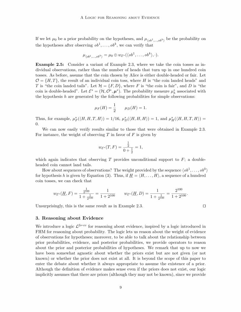
If we let µ0 be a prior probability on the hypotheses, and µ〈ob1,...,obk〉 be the probability onthe hypotheses after observing ob1, . . . , obk, we can verify that
µ〈ob1,...,obk〉 = µ0 ⊕ wE∗(〈ob1, . . . , obk〉, ·).
Example 2.5: Consider a variant of Example 2.3, where we take the coin tosses as in-dividual observations, rather than the number of heads that turn up in one hundred cointosses. As before, assume that the coin chosen by Alice is either double-headed or fair. LetO = {H,T}, the result of an individual coin toss, where H is “the coin landed heads” andT is “the coin landed tails”. Let H = {F,D}, where F is “the coin is fair”, and D is “thecoin is double-headed”. Let E∗ = (H,O∗,µ∗). The probability measure µ∗h associated withthe hypothesis h are generated by the following probabilities for simple observations:
µF (H) =12
µD(H) = 1.
Thus, for example, µ∗F (〈H,H, T,H〉) = 1/16, µ∗D(〈H,H,H〉) = 1, and µ∗H(〈H,H, T,H〉) =0.
We can now easily verify results similar to those that were obtained in Example 2.3.For instance, the weight of observing T in favor of F is given by
wE∗(T, F ) =12
0 + 12
= 1,
which again indicates that observing T provides unconditional support to F ; a double-headed coin cannot land tails.
How about sequences of observations? The weight provided by the sequence 〈ob1, . . . , obk〉for hypothesis h is given by Equation (3). Thus, if H = 〈H, . . . ,H〉, a sequence of a hundredcoin tosses, we can check that
wE∗(H,F ) =1
2100
1 + 12100
=1
1 + 2100wE∗(H,D) =
11 + 1
2100
=2100
1 + 2100.
Unsurprisingly, this is the same result as in Example 2.3. ut
3. Reasoning about Evidence
We introduce a logic Lfo-ev for reasoning about evidence, inspired by a logic introduced inFHM for reasoning about probability. The logic lets us reason about the weight of evidenceof observations for hypotheses; moreover, to be able to talk about the relationship betweenprior probabilities, evidence, and posterior probabilities, we provide operators to reasonabout the prior and posterior probabilities of hypotheses. We remark that up to now wehave been somewhat agnostic about whether the priors exist but are not given (or notknown) or whether the prior does not exist at all. It is beyond the scope of this paper toenter the debate about whether it always appropriate to assume the existence of a prior.Although the definition of evidence makes sense even if the priors does not exist, our logicimplicitly assumes that there are priors (although they may not be known), since we provide
9
Halpern & Pucella
operators for reasoning about the prior. We make use of these operators in some of theexamples below. However, the fragment of the logic that does not use these operators isappropriate for prior-free reasoning.
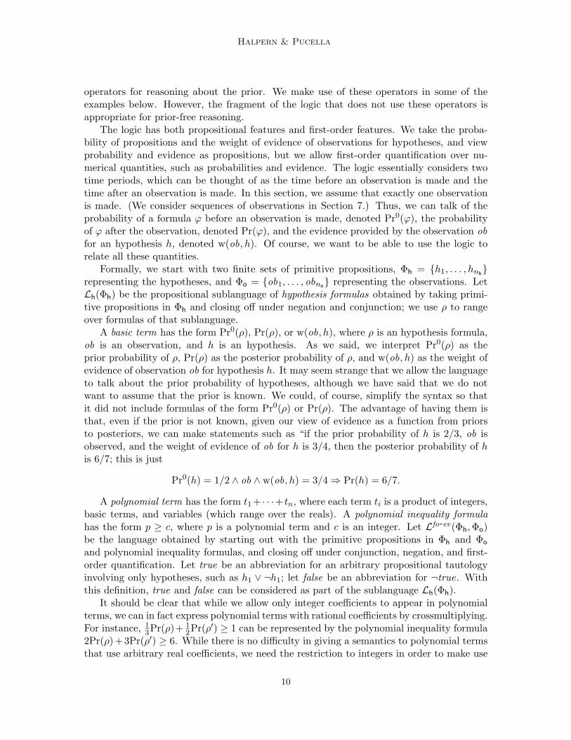
The logic has both propositional features and first-order features. We take the proba-bility of propositions and the weight of evidence of observations for hypotheses, and viewprobability and evidence as propositions, but we allow first-order quantification over nu-merical quantities, such as probabilities and evidence. The logic essentially considers twotime periods, which can be thought of as the time before an observation is made and thetime after an observation is made. In this section, we assume that exactly one observationis made. (We consider sequences of observations in Section 7.) Thus, we can talk of theprobability of a formula ϕ before an observation is made, denoted Pr0(ϕ), the probabilityof ϕ after the observation, denoted Pr(ϕ), and the evidence provided by the observation obfor an hypothesis h, denoted w(ob, h). Of course, we want to be able to use the logic torelate all these quantities.
Formally, we start with two finite sets of primitive propositions, Φh = {h1, . . . , hnh}
representing the hypotheses, and Φo = {ob1, . . . , obno} representing the observations. LetLh(Φh) be the propositional sublanguage of hypothesis formulas obtained by taking primi-tive propositions in Φh and closing off under negation and conjunction; we use ρ to rangeover formulas of that sublanguage.
A basic term has the form Pr0(ρ), Pr(ρ), or w(ob, h), where ρ is an hypothesis formula,ob is an observation, and h is an hypothesis. As we said, we interpret Pr0(ρ) as theprior probability of ρ, Pr(ρ) as the posterior probability of ρ, and w(ob, h) as the weight ofevidence of observation ob for hypothesis h. It may seem strange that we allow the languageto talk about the prior probability of hypotheses, although we have said that we do notwant to assume that the prior is known. We could, of course, simplify the syntax so thatit did not include formulas of the form Pr0(ρ) or Pr(ρ). The advantage of having them isthat, even if the prior is not known, given our view of evidence as a function from priorsto posteriors, we can make statements such as “if the prior probability of h is 2/3, ob isobserved, and the weight of evidence of ob for h is 3/4, then the posterior probability of his 6/7; this is just
Pr0(h) = 1/2 ∧ ob ∧ w(ob, h) = 3/4 ⇒ Pr(h) = 6/7.
A polynomial term has the form t1 + · · ·+ tn, where each term ti is a product of integers,basic terms, and variables (which range over the reals). A polynomial inequality formulahas the form p ≥ c, where p is a polynomial term and c is an integer. Let Lfo-ev (Φh,Φo)be the language obtained by starting out with the primitive propositions in Φh and Φo
and polynomial inequality formulas, and closing off under conjunction, negation, and first-order quantification. Let true be an abbreviation for an arbitrary propositional tautologyinvolving only hypotheses, such as h1 ∨ ¬h1; let false be an abbreviation for ¬true. Withthis definition, true and false can be considered as part of the sublanguage Lh(Φh).
It should be clear that while we allow only integer coefficients to appear in polynomialterms, we can in fact express polynomial terms with rational coefficients by crossmultiplying.For instance, 1
3Pr(ρ)+ 12Pr(ρ′) ≥ 1 can be represented by the polynomial inequality formula
2Pr(ρ)+3Pr(ρ′) ≥ 6. While there is no difficulty in giving a semantics to polynomial termsthat use arbitrary real coefficients, we need the restriction to integers in order to make use
10

A Logic for Reasoning about Evidence
of results from the theory of real closed fields in both the axiomatization of Section 4 andthe complexity results of Section 5.
We use obvious abbreviations where needed, such as ϕ ∨ ψ for ¬(¬ϕ ∧ ¬ψ), ϕ⇒ ψ for¬ϕ∨ψ, ∃xϕ for ¬∀x(¬ϕ), Pr(ϕ)−Pr(ψ) ≥ c for Pr(ϕ)+(−1)Pr(ψ) ≥ c, Pr(ϕ) ≥ Pr(ψ) forPr(ϕ)−Pr(ψ) ≥ 0, Pr(ϕ) ≤ c for −Pr(ϕ) ≥ −c, Pr(ϕ) < c for ¬(Pr(ϕ) ≥ c), and Pr(ϕ) = cfor (Pr(ϕ) ≥ c) ∧ (Pr(ϕ) ≤ c) (and analogous abbreviations for inequalities involving Pr0
and w).
Example 3.1: Consider again the situation given in Example 2.3. Let Φo, the observa-tions, consist of primitive propositions of the form heads[m], where m is an integer with0 ≤ m ≤ 100, indicating that m heads out of 100 tosses have appeared. Let Φh consistof the two primitive propositions fair and doubleheaded. The computations in Example 2.3can be written as follows:
w(heads[100], fair) = 1/(1 + 2100) ∧ w(heads[100], doubleheaded) = 2100/(1 + 2100).
We can also capture the fact that the weight of evidence of an observation maps a priorprobability into a posterior probability by Dempster’s Rule of Combination. For example,the following formula captures the update of the prior probability α of the hypothesis fairupon observation of a hundred coin tosses landing heads:
Pr0(fair) = α ∧ w(heads[100], fair) = 1/(1 + 2100) ⇒ Pr(fair) = α/(α+ (1− α)2100).
We develop a deductive system to derive such conclusions in the next section. ut
Now we consider the semantics. A formula is interpreted in a world that specifies whichhypothesis is true and which observation was made, as well as an evidence space to interpretthe weight of evidence of observations and a probability distribution on the hypotheses tointerpret prior probabilities and talk about updating based on evidence. (We do not needto include a posterior probability distribution, since it can be computed from the prior andthe weights of evidence using Equation (2).) An evidential world is a tuple w = (h, ob, µ, E),where h is a hypothesis, ob is an observation, µ is a probability distribution on Φh, and Eis an evidence space over Φh and Φo.
To interpret propositional formulas in Lh(Φh), we associate with each hypothesis formulaρ a set [[ρ]] of hypotheses, by induction on the structure of ρ:
[[h]] = {h}[[¬ρ]] = Φh − [[ρ]]
[[ρ1 ∧ ρ2]] = [[ρ1]] ∩ [[ρ2]].
To interpret first-order formulas that may contain variables, we need a valuation v thatassigns a real number to every variable. Given an evidential world w = (h, ob, µ, E) and avaluation v, we assign to a polynomial term p a real number [p]w,v in a straightforward way:
[x]w,v = v(x)[a]w,v = a
[Pr0(ρ)]w,v = µ([[ρ]])
11

Halpern & Pucella
[Pr(ρ)]w,v = (µ⊕ wE(ob, ·))([[ρ]])[w(ob ′, h′)]w,v = wE(ob ′, h′)
[t1t2]w,v = [t1]w,v × [t2]w,v
[p1 + p2]w,v = [p1]w,v + [p2]w,v.
Note that, to interpret Pr(ρ), the posterior probability of ρ after having observed ob (theobservation at world w), we use Equation (2), which says that the posterior is obtained bycombining the prior probability µ with wE(ob, ·).
We define what it means for a formula ϕ to be true (or satisfied) at an evidential worldw under valuation v, written (w, v) |= ϕ, as follows:
(w, v) |= h if w = (h, ob, µ, E) for some ob, µ, E
(w, v) |= ob if w = (h, ob, µ, E) for some h, µ, E
(w, v) |= ¬ϕ if (w, v) 6|= ϕ
(w, v) |= ϕ ∧ ψ if (w, v) |= ϕ and (w, v) |= ψ
(w, v) |= p ≥ c if [p]w,v ≥ c
(w, v) |= ∀xϕ if (w, v′) |= ϕ for all v′ that agree with v on all variables but x.
If (w, v) |= ϕ is true for all v, we write simply w |= ϕ. It is easy to check that if ϕis a closed formula (that is, one with no free variables), then (w, v) |= ϕ if and only if(w, v′) |= ϕ, for all v, v′. Therefore, given a closed formula ϕ, if (M,w, v) |= ϕ, then in factw |= ϕ. We will typically be concerned only with closed formulas. Finally, if w |= ϕ forall evidential worlds w, we write |= ϕ and say that ϕ is valid. In the next section, we willcharacterize axiomatically all the valid formulas of the logic.
Example 3.2: The following formula is valid, that is, true in all evidential worlds:
|= (w(ob, h1) = 2/3 ∧ w(ob, h2) = 1/3) ⇒ (Pr0(h1) ≥ 1/100 ∧ ob) ⇒ Pr(h1) ≥ 2/101.
In other words, at all evidential worlds where the weight of evidence of observation ob forhypothesis h1 is 2/3 and the weight of evidence of observation ob for hypothesis h2 is 1/3,it must be the case that if the prior probability of h1 is at least 1/100 and ob is actuallyobserved, then the posterior probability of h1 is at least 2/101. This shows the extent towhich we can reason about the evidence independently of the prior probabilities. ut
The logic imposes no restriction on the prior probabilities to be used in the models.This implies, for instance, that the formula
fair ⇒ Pr0(fair) = 0
is satisfiable: there exists an evidential world w such that the formula is true at w. In otherwords, it is consistent for an hypothesis to be true, despite the prior probability of it beingtrue being 0. It is a simple matter to impose a restriction on the models that they be suchthat if h is true at a world, then µ(h) > 0 for the prior µ at that world.
12

A Logic for Reasoning about Evidence
We conclude this section with some remarks concerning the semantic model. Our se-mantic model implicitly assumes that the prior probability is known and that the likelihoodfunctions (i.e., the measures µh) are known. Of course, in many situations there will beuncertainty about both. Indeed, our motivation for focusing on evidence is precisely to dealwith situations where the prior is not known. Handling uncertainty about the prior is easyin our framework, since our notion of evidence is independent of the prior on hypotheses. Itis straightforward to extend our model by allowing a set of possible worlds, with a differentprior in each, but using the same evidence space for all of them. We can then extend thelogic with a knowledge operator, where a statement is known to be true if it is true in allthe worlds. This allows us to make statements like “I know that the prior on hypothesish is between α and β. Since observation ob provides evidence 3/4 for h, I know that theposterior on h given ob is between (3α)/(2α+ 1) and (3β)/(2β + 1).”
Dealing with uncertainty about the likelihood functions is somewhat more subtle. Tounderstand the issue, suppose that one of two coins will be chosen and tossed. The bias ofcoin 1 (i.e., the probability that coin 1 lands heads) is between 2/3 and 3/4; the bias of coin2 is between 1/4 and 1/3. Here there is uncertainty about the probability that coin 1 willbe picked (this is uncertainty about the prior) and there is uncertainty about the bias ofeach coin (this is uncertainty about the likelihood functions). The problem here is that, todeal with this, we must consider possible worlds where there is a possibly different evidencespace in each world. It is then not obvious how to define weight of evidence. We explorethis issue in more detail in a companion paper (Halpern & Pucella, 2005a).
4. Axiomatizing Evidence
In this section we present a sound and complete axiomatization AX(Φh,Φo) for our logic.The axiomatization can be divided into four parts. The first part, consisting of the
following axiom and inference rule, accounts for first-order reasoning:
Taut. All substitution instances of valid formulas of first-order logic with equality.
MP. From ϕ and ϕ⇒ ψ infer ψ.
Instances of Taut include, for example, all formulas of the form ϕ ∨ ¬ϕ, where ϕ is anarbitrary formula of the logic. It also includes formulas such as (∀xϕ) ⇔ ϕ if x is not freein ϕ. In particular, (∀x(h)) ⇔ h for hypotheses in Φh, and similarly for observations inΦo. Note that Taut includes all substitution instances of valid formulas of first-order logicwith equality; in other words, any valid formula of first-order logic with equality wherefree variables are replaced with arbitrary terms of our language (including Pr0(ρ), Pr(ρ),w(ob, h)) is an instance of Taut. Axiom Taut can be replaced by a sound and completeaxiomatization for first-order logic with equality, as given, for instance, in Shoenfield (1967)or Enderton (1972).
The second set of axioms accounts for reasoning about polynomial inequalities, by relyingon the theory of real closed fields:
RCF. All instances of formulas valid in real closed fields (and, thus, true about the reals),with nonlogical symbols +, ·, <, 0, 1, −1, 2, −2, 3, −3, . . . .
13
Halpern & Pucella
Formulas that are valid in real closed fields include, for example, the fact that addition on thereals is associative, ∀x∀y∀z((x+y)+z = x+(y+z)), that 1 is the identity for multiplication,∀x(x·1 = x), and formulas relating the constant symbols, such as k = 1+· · ·+1 (k times) and−1 + 1 = 0. As for Taut, we could replace RCF by a sound and complete axiomatizationfor real closed fields (cf. Fagin et al., 1990; Shoenfield, 1967; Tarski, 1951).
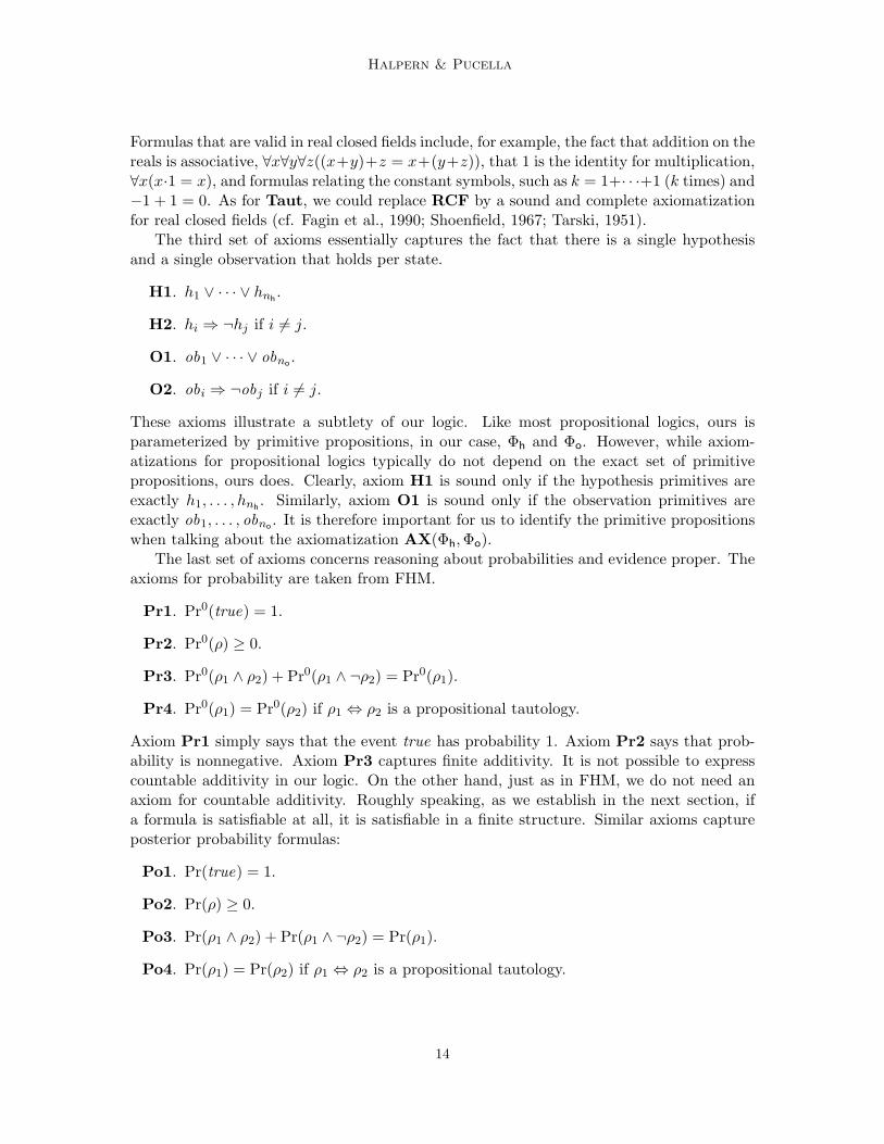
The third set of axioms essentially captures the fact that there is a single hypothesisand a single observation that holds per state.
H1. h1 ∨ · · · ∨ hnh.
H2. hi ⇒ ¬hj if i 6= j.
O1. ob1 ∨ · · · ∨ obno .
O2. obi ⇒ ¬obj if i 6= j.
These axioms illustrate a subtlety of our logic. Like most propositional logics, ours isparameterized by primitive propositions, in our case, Φh and Φo. However, while axiom-atizations for propositional logics typically do not depend on the exact set of primitivepropositions, ours does. Clearly, axiom H1 is sound only if the hypothesis primitives areexactly h1, . . . , hnh
. Similarly, axiom O1 is sound only if the observation primitives areexactly ob1, . . . , obno . It is therefore important for us to identify the primitive propositionswhen talking about the axiomatization AX(Φh,Φo).
The last set of axioms concerns reasoning about probabilities and evidence proper. Theaxioms for probability are taken from FHM.
Pr1. Pr0(true) = 1.
Pr2. Pr0(ρ) ≥ 0.
Pr3. Pr0(ρ1 ∧ ρ2) + Pr0(ρ1 ∧ ¬ρ2) = Pr0(ρ1).
Pr4. Pr0(ρ1) = Pr0(ρ2) if ρ1 ⇔ ρ2 is a propositional tautology.
Axiom Pr1 simply says that the event true has probability 1. Axiom Pr2 says that prob-ability is nonnegative. Axiom Pr3 captures finite additivity. It is not possible to expresscountable additivity in our logic. On the other hand, just as in FHM, we do not need anaxiom for countable additivity. Roughly speaking, as we establish in the next section, ifa formula is satisfiable at all, it is satisfiable in a finite structure. Similar axioms captureposterior probability formulas:
Po1. Pr(true) = 1.
Po2. Pr(ρ) ≥ 0.
Po3. Pr(ρ1 ∧ ρ2) + Pr(ρ1 ∧ ¬ρ2) = Pr(ρ1).
Po4. Pr(ρ1) = Pr(ρ2) if ρ1 ⇔ ρ2 is a propositional tautology.
14
A Logic for Reasoning about Evidence
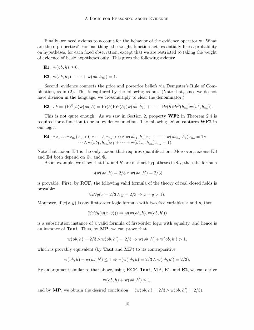
Finally, we need axioms to account for the behavior of the evidence operator w. Whatare these properties? For one thing, the weight function acts essentially like a probabilityon hypotheses, for each fixed observation, except that we are restricted to taking the weightof evidence of basic hypotheses only. This gives the following axioms:
E1. w(ob, h) ≥ 0.
E2. w(ob, h1) + · · ·+ w(ob, hnh) = 1.
Second, evidence connects the prior and posterior beliefs via Dempster’s Rule of Com-bination, as in (2). This is captured by the following axiom. (Note that, since we do nothave division in the language, we crossmultiply to clear the denominator.)
E3. ob ⇒ (Pr0(h)w(ob, h) = Pr(h)Pr0(h1)w(ob, h1) + · · ·+ Pr(h)Pr0(hnh)w(ob, hnh
)).
This is not quite enough. As we saw in Section 2, property WF2 in Theorem 2.4 isrequired for a function to be an evidence function. The following axiom captures WF2 inour logic:
E4. ∃x1 . . .∃xno(x1 > 0 ∧ · · · ∧ xno > 0 ∧ w(ob1, h1)x1 + · · ·+ w(obno , h1)xno = 1∧· · · ∧ w(ob1, hnh
)x1 + · · ·+ w(obno , hnh)xno = 1).
Note that axiom E4 is the only axiom that requires quantification. Moreover, axioms E3and E4 both depend on Φh and Φo.
As an example, we show that if h and h′ are distinct hypotheses in Φh, then the formula
¬(w(ob, h) = 2/3 ∧ w(ob, h′) = 2/3)
is provable. First, by RCF, the following valid formula of the theory of real closed fields isprovable:
∀x∀y(x = 2/3 ∧ y = 2/3 ⇒ x+ y > 1).
Moreover, if ϕ(x, y) is any first-order logic formula with two free variables x and y, then
(∀x∀y(ϕ(x, y))) ⇒ ϕ(w(ob, h),w(ob, h′))
is a substitution instance of a valid formula of first-order logic with equality, and hence isan instance of Taut. Thus, by MP, we can prove that
w(ob, h) = 2/3 ∧ w(ob, h′) = 2/3 ⇒ w(ob, h) + w(ob, h′) > 1,
which is provably equivalent (by Taut and MP) to its contrapositive
w(ob, h) + w(ob, h′) ≤ 1 ⇒ ¬(w(ob, h) = 2/3 ∧ w(ob, h′) = 2/3).
By an argument similar to that above, using RCF, Taut, MP, E1, and E2, we can derive
w(ob, h) + w(ob, h′) ≤ 1,
and by MP, we obtain the desired conclusion: ¬(w(ob, h) = 2/3 ∧ w(ob, h′) = 2/3).
15
Halpern & Pucella
Theorem 4.1: AX(Φh,Φo) is a sound and complete axiomatization for Lfo-ev (Φh,Φo)with respect to evidential worlds.
As usual, soundness is straightforward, and to prove completeness, it suffices to showthat if a formula ϕ is consistent with AX(Φh,Φo), it is satisfiable in an evidential struc-ture. However, the usual approach for proving completeness in modal logic, which involvesconsidering maximal consistent sets and canonical structures does not work. The problemis that there are maximal consistent sets of formulas that are not satisfiable. For example,there is a maximal consistent set of formulas that includes Pr(ρ) > 0 and Pr(ρ) ≤ 1/n forn = 1, 2, . . . . This is clearly unsatisfiable. Our proof follows the techniques developed inFHM.
To express axiom E4, we needed to have quantification in the logic. This is where thefact that our representation of evidence is normalized has a nontrivial effect on the logic: E4corresponds to property WF2, which essentially says that a function is a weight of evidencefunction if one can find such a normalization factor. An interesting question is whether itis possible to find a sound and complete axiomatization for the propositional fragment ofour logic (without quantification or variables). To do this, we need to give quantifier-freeaxioms to replace axiom E4. This amounts to asking whether there is a simpler propertythan WF2 in Theorem 2.4 that characterizes weight of evidence functions. This remainsan open question.
5. Decision Procedures
In this section, we consider the decision problem for our logic, that is, the problem ofdeciding whether a given formula ϕ is satisfiable. In order to state the problem precisely,however, we need to deal carefully with the fact that the logic is parameterized by the setsΦh and Φo of primitive propositions representing hypotheses and observations. In mostlogics, the choice of underlying primitive propositions is essentially irrelevant. For example,if a propositional formula ϕ that contains only primitive propositions in some set Φ istrue with respect to all truth assignments to Φ, then it remains true with respect to alltruth assignments to any set Φ′ ⊇ Φ. This monotonicity property does not hold here. Forexample, as we have already observed, axiom H1 clearly depends on the set of hypothesesand observations; it is no longer valid if the set is changed. The same is true for O1, E3,and E4.
This means that we have to be careful, when stating decision problems, about the roleof Φh and Φo in the algorithm. A straightforward way to deal with this is to assume thatthe satisfiability algorithm gets as input Φh, Φo, and a formula ϕ ∈ Lfo-ev (Φh,Φo). BecauseLfo-ev (Φh,Φo) contains the full theory of real closed fields, it is unsurprisingly difficult todecide. For our decision procedure, we can use the exponential-space algorithm of Ben-Or,Kozen, and Reif (1986) to decide the satisfiability of real closed field formulas. We definethe length |ϕ| of ϕ to be the number of symbols required to write ϕ, where we count thelength of each coefficient as 1. Similarly, we define ‖ϕ‖ to be the length of the longestcoefficient appearing in f , when written in binary.
Theorem 5.1: There is a procedure that runs in space exponential in |ϕ| ‖ϕ‖ for deciding,given Φh and Φo, whether a formula ϕ of Lfo-ev (Φh,Φo) is satisfiable in an evidential world.
16
A Logic for Reasoning about Evidence
This is essentially the best we can do, since Ben-Or, Kozen, and Reif (1986) prove thatthe decision problem for real closed fields is complete for exponential space, and our logiccontains the full language of real closed fields.
While we assumed that the algorithm takes as input the set of primitive propositionsΦh and Φo, this does not really affect the complexity of the algorithm. More precisely, ifwe are given a formula ϕ in Lfo-ev over some set of hypotheses and observations, we canstill decide whether ϕ is satisfiable, that is, whether there are sets Φh and Φo of primitivepropositions containing all the primitive propositions in ϕ and an evidential world w thatsatisfies ϕ.
Theorem 5.2: There is a procedure that runs in space exponential in |ϕ| ‖ϕ‖ for decidingwhether there exists sets of primitive propositions Φh and Φo such that ϕ ∈ Lfo-ev (Φh,Φo)and ϕ is satisfiable in an evidential world.
The main culprit for the exponential-space complexity is the theory of real closed fields,which we had to add to the logic to be able to even write down axiom E4 of the axioma-tization AX(Φh,Φo).5 However, if we are not interested in axiomatizations, but simply inverifying properties of probabilities and weights of evidence, we can consider the followingpropositional (quantifier-free) fragment of our logic. As before, we start with sets Φh andΦo of hypothesis and observation primitives, and form the sublanguage Lh of hypothesisformulas. Basic terms have the form Pr0(ρ), Pr(ρ), and w(ob, h), where ρ is an hypothesisformula, ob is an observation, and h is an hypothesis. A quantifier-free polynomial termhas the form a1t1 + · · · + antn, where each ai is an integer and each ti is a product ofbasic terms. A quantifier-free polynomial inequality formula has the form p ≥ c, wherep is a quantifier-free polynomial term, and c is an integer. For instance, a quantifier-freepolynomial inequality formula takes the form Pr0(ρ) + 3w(ob, h) + 5Pr0(ρ)Pr(ρ′) ≥ 7.
Let Lev (Φh,Φo) be the language obtained by starting out with the primitive propositionsin Φh and Φo and quantifier-free polynomial inequality formulas, and closing off under con-junction and negation. Since quantifier-free polynomial inequality formulas are polynomialinequality formulas, Lev (Φh,Φo) is a sublanguage of Lfo-ev (Φh,Φo). The logic Lev (Φh,Φo)is sufficiently expressive to express many properties of interest; for instance, it can certainlyexpress the general connection between priors, posteriors, and evidence captured by axiomE3, as well as specific relationships between prior probability and posterior probabilitythrough the weight of evidence of a particular observation, as in Example 3.1. Reasoningabout the propositional fragment of our logic Lev (Φh,Φo) is easier than the full language.6
5. Recall that axiom E4 requires existential quantification. Thus, we can restrict to the sublanguageconsisting of formulas with a single block of existential quantifiers in prefix position. The satisfiabilityproblem for this sublanguage can be shown to be decidable in time exponential in the size of the formula(Renegar, 1992).
6. In a preliminary version of this paper (Halpern & Pucella, 2003), we examined the quantifier-free fragmentof Lfo-ev (Φh, Φo) that uses only linear inequality formulas, of the form a1t1 + · · ·+ antn ≥ c, where eachti is a basic term. We claimed that the problem of deciding, given Φh and Φo, whether a formula ϕ ofthis fragment is satisfiable in an evidential world is NP-complete. We further claimed that this resultfollowed from a small-model theorem: if ϕ is satisfiable, then it is satisfiable in an evidential world overa small number of hypotheses and observations. While this small-model theorem is true, our argumentthat the satisfiability problem is in NP also implicitly assumed that the numbers associated with theprobability measure and the evidence space in the evidential world were small. But this is not true
17
Halpern & Pucella
Theorem 5.3: There is a procedure that runs in space polynomial in |ϕ| ‖ϕ‖ for deciding,given Φh and Φo, whether a formula ϕ of Lev (Φh,Φo) is satisfiable in an evidential world.
Theorem 5.3 relies on Canny’s (1988) procedure for deciding the validity of quantifier-free formulas in the theory of real closed fields. As in the general case, the complexity isunaffected by whether or not the decision problem takes as input the sets Φh and Φo ofprimitive propositions.
Theorem 5.4: There is a procedure that runs in space polynomial in |ϕ| ‖ϕ‖ for decidingwhether there exists sets of primitive propositions Φh and Φo such that ϕ ∈ Lev (Φh,Φo) andϕ is satisfiable in an evidential world.
6. Normalized Versus Unnormalized Likelihoods
The weight of evidence we used throughout this paper is a generalization of the log-likelihoodratio advocated by Good (1950, 1960). As we pointed out earlier, this measure of confirma-tion is essentially a normalized likelihood: the likelihood of an observation given a particularhypothesis is normalized by the sum of all the likelihoods of that observation, for all possi-ble hypotheses. What would change if we were to take the (unnormalized) likelihoods µh
themselves as weight of evidence? Some things would simplify. For example, WF2 is aconsequence of normalization, as is the corresponding axiom E4, which is the only axiomthat requires quantification.
The main argument for normalizing likelihood is the same as that for normalizing prob-ability measures. Just like probability, when using normalized likelihood, the weight ofevidence is always between 0 and 1, and provides an absolute scale against which to judgeall reports of evidence. The impact here is psychological—it permits one to use the samerules of thumb in all situations, since the numbers obtained are independent from the con-text of their use. Thus, for instance, a weight of evidence of 0.95 in one situation correspondsto the “same amount” of evidence as a weight of evidence of 0.95 in a different situation;any acceptable decision based on this weight of evidence in the first situation ought to beacceptable in the other situation as well. The importance of having such a uniform scaledepends, of course, on the intended applications.
For the sake of completeness, we now describe the changes to our framework requiredto use unnormalized likelihoods as a weight of evidence. Define wu
E(ob, h) = µh(ob).
in general. Even though the formula ϕ involves only linear inequality formulas, every evidential worldsatisfies axiom E3. This constraint enables us to write formulas for which there exist no models wherethe probabilities and weights of evidence are rational. For example, consider the formula
Pr0(h1) = w(ob1, h1) ∧ Pr0(h2) = 1− Pr0(h1) ∧ Pr(h1) = 1/2 ∧ w(ob1, h2) = 1/4
Any evidential world satisfying the formula must satisfy
Pr0(h1) = w(ob1, h1) = −1/8(1−√
17)
which is irrational. The exact complexity of this fragment remains open. We can use our techniques toshow that it is in PSPACE, but we have no matching lower bound. (In particular, it may indeed be inNP.) We re-examine this fragment of the logic in Section 6, under a different interpretation of weightsof evidence.
18
A Logic for Reasoning about Evidence
First, note that we can update a prior probability µ0 via a set of likelihood functions µh
using a form of Dempster’s Rule of Combination. More precisely, we can define µ0⊕wuE(ob, ·)
to be the probability measure defined by
(µ0 ⊕ wuE(ob, ·))(h) =
µ0(h)µh(ob)∑h′∈H µ0(h′)µh′(ob)
.
The logic we introduced in Section 3 applies just as well to this new interpretation ofweights of evidence. The syntax remains unchanged, the models remain evidential worlds,and the semantics of formulas simply take the new interpretation of weight of evidenceinto account. In particular, the assignment [p]w,v now uses the above definition of wu
E , andbecomes
[Pr(ρ)]w,v = (µ⊕ wuE(ob, ·))([[ρ]])
[w(ob ′, h′)]w,v = wuE(ob
′, h′).
The axiomatization of this new logic is slightly different and somewhat simpler than theone in Section 3. In particular, E1 and E2, which say that w(ob, h) acts as a probabilitymeasure for each fixed ob, are replaced by axioms that say that w(ob, h) acts as a probabilitymeasure for each fixed h:
E1′. w(ob, h) ≥ 0.
E2′. w(ob1, h) + · · ·+ w(obno , h) = 1.
Axiom E3 is unchanged, since wuE is updated in essentially the same way as wE . Axiom E4
becomes unnecessary.What about the complexity of the decision procedure? As in Section 5, the complexity
of the decision problem for the full logic Lfo-ev (Φh,Φo) remains dominated by the complex-ity of reasoning in real closed fields. Of course, now, we can express the full axiomatizationfor the unnormalized likelihood interpretation of weight of evidence in the Lev (Φh,Φo) frag-ment, which can be decided in polynomial space. A further advantage of the unnormalizedlikelihood interpretation of weight of evidence, however, is that it leads to a useful fragmentof Lev (Φh,Φo) that is perhaps easier to decide.
Suppose that we are interested in reasoning exclusively about weights of evidence, withno prior or posterior probability. This is the kind of reasoning that actually underliesmany computer science applications involving randomized algorithms (Halpern & Pucella,2005b). As before, we start with sets Φh and Φo of hypothesis and observation primitives,and form the sublanguage Lh of hypothesis formulas. A quantifier-free linear term hasthe form a1w(ob1, h1) + · · · + anw(obn, hn), where each ai is an integer, each obi is anobservation, and each hi is an hypothesis. A quantifier-free linear inequality formula hasthe form p ≥ c, where p is a quantifier-free linear term and c is an integer. For example,w(ob ′, h) + 3w(ob, h) ≥ 7 is a quantifier-free linear inequality formula.
Let Lw (Φh,Φo) be the language obtained by starting out with the primitive propositionsin Φh and Φo and quantifier-free linear inequality formulas, and closing off under conjunctionand negation. Since quantifier-free linear inequality formulas are polynomial inequalityformulas, Lw (Φh,Φo) is a sublanguage of Lfo-ev (Φh,Φo). Reasoning about Lw (Φh,Φo) iseasier than the full language, and possibly easier than the Lev (Φh,Φo) fragment.
19

Halpern & Pucella
Theorem 6.1: The problem of deciding, given Φh and Φo, whether a formula ϕ of Lw (Φh,Φo)is satisfiable in an evidential world is NP-complete.
As in the general case, the complexity is unaffected by whether or not the decisionproblem takes as input the sets Φh and Φo of primitive propositions.
Theorem 6.2: The problem of deciding, for a formula ϕ, whether there exists sets ofprimitive propositions Φh and Φo such that ϕ ∈ Lw (Φh,Φo) and ϕ is satisfiable in anevidential world is NP-complete.
7. Evidence in Dynamic Systems
The evidential worlds we have considered until now are essentially static, in that they modelonly the situation where a single observation is made. Considering such static worlds letsus focus on the relationship between the prior and posterior probabilities on hypothesesand the weight of evidence of a single observation. In a related paper (Halpern & Pucella,2005b), we consider evidence in the context of randomized algorithms; we use evidence tocharacterize the information provided by, for example, a randomized algorithm for primalitywhen it says that a number is prime. The framework in that work is dynamic; sequences ofobservations are made over time. In this section, we extend our logic to reason about theevidence of sequences of observations, using the approach to combining evidence describedin Section 2.
There are subtleties involved in trying to find an appropriate logic for reasoning aboutsituations like that in Example 2.5. The most important one is the relationship betweenobservations and time. By way of illustration, consider the following example. Bob isexpecting an email from Alice stating where a rendezvous is to take place. Calm underpressure, Bob is reading while he waits. We assume that Bob is not concerned with thetime. For the purposes of this example, one of three things can occur at any given point intime:
(1) Bob does not check if he has received email;
(2) Bob checks if he has received email, and notices he has not received an email fromAlice;
(3) Bob checks if he has received email, and notices he has received an email from Alice.
How is his view of the world affected by these events? In (1), it should be clear that,all things being equal, Bob’s view of the world does not change: no observation is made.Contrast this with (2) and (3). In (2), Bob does make an observation, namely that he hasnot yet received Alice’s email. The fact that he checks indicates that he wants to observe aresult. In (3), he also makes an observation, namely that he received an email from Alice.In both of these cases, the check yields an observation, that he can use to update his viewof the world. In case (2), he essentially observed that nothing happened, but we emphasizeagain that this is an observation, to be distinguished from the case where Bob does noteven check whether email has arrived, and should be explicit in the set O in the evidencespace.
20
A Logic for Reasoning about Evidence
This discussion motivates the models that we use in this section. We characterizean agent’s state by the observations that she has made, including possibly the “nothinghappened” observation. Although we do not explicitly model time, it is easy to incorporatetime in our framework, since the agent can observe times or clock ticks. The models in thissection are admittedly simple, but they already highlight the issues involved in reasoningabout evidence in dynamic systems. As long as agents do not forget observations, there isno loss of generality in associating an agent’s state with a sequence of observations. We do,however, make the simplifying assumption that the same evidence space is used for all theobservations in a sequence. In other words, we assume that the evidence space is fixed forthe evolution of the system. In many situations of interest, the external world changes. Thepossible observations may depend on the state of the world, as may the likelihood functions.There are no intrinsic difficulties in extending the model to handle state changes, but theadditional details would only obscure the presentation.
In some ways, considering a dynamic setting simplifies things. Rather than talkingabout the prior and posterior probability using different operators, we need only a singleprobability operator that represents the probability of an hypothesis at the current time.To express the analogue of axiom E3 in this logic, we need to be able to talk about theprobability at the next time step. This can be done by adding the “next-time” operator© to the logic, where ©ϕ holds at the current time if ϕ holds at the next time step.7 Wefurther extend the logic to talk about the weight of evidence of a sequence of observations.
We define the logic Lfo-evdyn as follows. As in Section 3, we start with a set of primitive
propositions Φh and Φo, respectively representing the hypotheses and the observations.Again, let Lh(Φh) be the propositional sublanguage of hypotheses formulas obtained bytaking primitive propositions in Φh and closing off under negation and conjunction; we useρ to range over formulas of that sublanguage.
A basic term now has the form Pr(ρ) or w(ob, h), where ρ is an hypothesis formula,ob = 〈ob1, . . . , obk〉 is a nonempty sequence of observations, and h is an hypothesis. Ifob = 〈ob1〉, we write w(ob1, h) rather than w(〈ob1〉, h). As before, a polynomial term hasthe form t1 + · · ·+ tn, where each term ti is a product of integers, basic terms, and variables(which intuitively range over the reals). A polynomial inequality formula has the formp ≥ c, where p is a polynomial term and c is an integer. Let Lfo-ev
dyn (Φh,Φo) be the languageobtained by starting out with the primitive propositions in Φh and Φo and polynomialinequality formulas, and closing off under conjunction, negation, first-order quantification,and application of the © operator. We use the same abbreviations as in Section 3.
The semantics of this logic now involves models that have dynamic behavior. Ratherthan just considering individual worlds, we now consider sequences of worlds, which wecall runs, representing the evolution of the system over time. A model is now an infiniterun, where a run describes a possible dynamic evolution of the system. As before, a runrecords the observations being made and the hypothesis that is true for the run, as well asa probability distribution describing the prior probability of the hypothesis at the initialstate of the run, and an evidence space E∗ over Φh and Φ∗
o to interpret w. We define anevidential run r to be a map from the natural numbers (representing time) to histories of
7. Following the discussion above, time steps are associated with new observations. Thus, ©ϕ means thatϕ is true at the next time step, that is, after the next observation. This simplifies the presentation ofthe logic.
21
Halpern & Pucella
the system up to that time. A history at time m records the relevant information about therun—the hypothesis that is true, the prior probability on the hypotheses, and the evidencespace E∗—and the observations that have been made up to time m. Hence, a history hasthe form 〈(h, µ, E∗), ob1, . . . , obk〉. We assume that r(0) = 〈(h, µ, E∗)〉 for some h, µ, andE∗, while r(m) = 〈(h, µ, E∗), ob1, . . . , obm〉 for m > 0. We define a point of the run to be apair (r,m) consisting of a run r and time m.
We associate with each propositional formula ρ in Lh(Φh) a set [[ρ]] of hypotheses, justas we did in Section 3.
In order to ascribe a semantics to first-order formulas that may contain variables, weneed a valuation v that assigns a real number to every variable. Given a valuation v, anevidential run r, and a point (r,m), where r(m) = 〈(h, µ, E∗), ob1, . . . , obm〉, we can assignto a polynomial term p a real number [p]r,m,v using essentially the same approach as inSection 3:
[x]r,m,v = v(x)[a]r,m,v = a
[Pr(ρ)]r,m,v = (µ⊕ wE∗(〈ob1, . . . , obm〉, ·)))([[ρ]])where r(m) = 〈(h, µ, E∗), ob1, . . . , obm〉
[w(ob, h′)]r,m,v = wE∗(ob, h′)where r(m) = 〈(h, µ, E∗), ob1, . . . , obm〉
[t1t2]r,m,v = [t1]r,m,v × [t2]r,m,v
[p1 + p2]r,m,,v = [p1]r,m,v + [p2]r,m,v.
We define what it means for a formula ϕ to be true (or satisfied) at a point (r,m) ofan evidential run r under valuation v, written (r,m, v) |= ϕ, using essentially the sameapproach as in Section 3:
(r,m, v) |= h if r(m) = 〈(h, µ, E∗), . . .〉
(r,m, v) |= ob if r(m) = 〈(h, µ, E∗), . . . , ob〉
(r,m, v) |= ¬ϕ if (r,m, v) 6|= ϕ
(r,m, v) |= ϕ ∧ ψ if (r,m, v) |= ϕ and (r,m, v) |= ψ
(r,m, v) |= p ≥ c if [p]r,m,v ≥ c
(r,m, v) |= ©ϕ if (r,m+ 1, v) |= ϕ
(r,m, v) |= ∀xϕ if (r,m, v′) |= ϕ for all valuations v′ that agree with v on all variablesbut x.
If (r,m, v) |= ϕ is true for all v, we simply write (r,m) |= ϕ. If (r,m) |= ϕ for all points(r,m) of r, then we write r |= ϕ and say that ϕ is valid in r. Finally, if r |= ϕ for allevidential runs r, we write |= ϕ and say that ϕ is valid.
It is straightforward to axiomatize this new logic. The axiomatization shows that wecan capture the combination of evidence directly in the logic, a pleasant property. Most of
22
A Logic for Reasoning about Evidence
the axioms from Section 3 carry over immediately. Let the axiomatization AXdyn(Φh,Φo)consists of the following axioms and inference rules: first-order reasoning (Taut, MP), rea-soning about polynomial inequalities (RCF), reasoning about hypotheses and observations(H1,H2,O1,O2), reasoning about probabilities (Po1–4 only, since we do not have Pr0 inthe language), and reasoning about weights of evidence (E1, E2, E4), as well as new axiomswe now present.
Basically, the only axiom that needs replacing is E3, which links prior and posteriorprobabilities, since this now needs to be expressed using the © operator. Moreover, weneed an axiom to relate the weight of evidence of a sequence of observation to the weightof evidence of the individual observations, as given by Equation (3).
E5. ob ⇒ ∀x(©(Pr(h) = x) ⇒Pr(h)w(ob, h) = xPr(h1)w(ob, h1) + · · ·+ xPr(hnh
)w(ob, hnh)).
E6. w(ob1, h) · · ·w(obk, h) = w(〈ob1, . . . , obk〉, h)w(ob1, h1) · · ·w(obk, h1) + · · ·+w(〈ob1, . . . , obk〉, h)w(ob1, hnh
) · · ·w(obk, hnh).
To get a complete axiomatization, we also need axioms and inference rules that capturethe properties of the temporal operator ©.
T1. ©ϕ ∧©(ϕ⇒ ψ) ⇒ ©ψ.
T2. ©¬ϕ⇔ ¬©ϕ.
T3. From ϕ infer ©ϕ.
Finally, we need axioms to say that the truth of hypotheses as well as the value of polynomialterms not containing occurrences of Pr is time-independent:
T4. ©ρ⇔ ρ.
T5. ©(p ≥ c) ⇔ p ≥ c if p does not contain an occurrence of Pr.
T6. ©(∀xϕ) ⇔ ∀x(©ϕ).
Theorem 7.1: AXdyn(Φh,Φo) is a sound and complete axiomatization for Lfo-evdyn (Φh,Φo)
with respect to evidential runs.
8. Conclusion
In the literature, reasoning about the effect of observations is typically done in a contextwhere we have a prior probability on a set of hypotheses which we can condition on theobservations made to obtain a new probability on the hypotheses that reflects the effect ofthe observations. In this paper, we have presented a logic of evidence that lets us reasonabout the weight of evidence of observations, independently of any prior probability on thehypotheses. The logic is expressive enough to capture in a logical form the relationshipbetween a prior probability on hypotheses, the weight of evidence of observations, and theresult posterior probability on hypotheses. But we can also capture reasoning that does notinvolve prior probabilities.
23

Halpern & Pucella
While the logic is essentially propositional, obtaining a sound and complete axiomati-zation seems to require quantification over the reals. This adds to the complexity of thelogic—the decision problem for the full logic is in exponential space. However, an interest-ing and potentially useful fragment, the propositional fragment, is decidable in polynomialspace.
Acknowledgments. A preliminary version of this paper appeared in the Proceedings ofthe Nineteenth Conference on Uncertainty in Artificial Intelligence, pp. 297–304, 2003. Thiswork was mainly done while the second author was at Cornell University. We thank DexterKozen and Nimrod Megiddo for useful discussions. Special thanks to Manfred Jaeger forhis careful reading of the paper and subsequent comments. Manfred found the bug in ourproof that the satisfiability problem for the quantifier-free fragment of Lfo-ev (Φh,Φo) thatuses only linear inequality formulas is NP-complete. His comments also led us to discuss theissue of normalization. We also thank the reviewers, whose comments greatly improved thepaper. This work was supported in part by NSF under grants CTC-0208535, ITR-0325453,and IIS-0534064, by ONR under grant N00014-01-10-511, by the DoD MultidisciplinaryUniversity Research Initiative (MURI) program administered by the ONR under grantsN00014-01-1-0795 and N00014-04-1-0725, and by AFOSR under grant F49620-02-1-0101.
Appendix A. Proofs
Proposition 2.1: For all ob, we have wE(ob, hi) ≥ wE(ob, h3−i) if and only if l(ob, hi) ≥l(ob, h3−i), for i = 1, 2, and for all h, ob, and ob ′, we have wE(ob, h) ≥ wE(ob ′, h) if andonly if l(ob, h) ≥ l(ob ′, h).
Proof. Let ob be an arbitrary observation. The result follows from the following argument:
wE(ob, hi) ≥ wE(ob, h3−i)iff µhi
(ob)/(µhi(ob) + µh3−i
(ob)) ≥ µh3−i(ob)/(µhi
(ob) + µh3−i(ob))
iff µhi(ob)µhi
(ob) ≥ µh3−i(ob)µh3−i
(ob)iff µhi
(ob)/µh3−i(ob) ≥ µh3−i
(ob)/µhi(ob)
iff l(ob, hi) ≥ l(ob, h3−i).
A similar argument establishes the result for hypotheses. ut
Theorem 2.4: Let H = {h1, . . . , hm} and O = {ob1, . . . , obn}, and let f be a real-valuedfunction with domain O×H such that f(ob, h) ∈ [0, 1]. Then there exists an evidence spaceE = (H,O, µh1 , . . . , µhm) such that f = wE if and only if f satisfies the following properties:
WF1. For every ob ∈ O, f(ob, ·) is a probability measure on H.
WF2. There exists x1, . . . , xn > 0 such that, for all h ∈ H,∑n
i=1 f(obi, h)xi = 1.
Proof. (⇒) Assume that f = wE for some evidence space E = (H,O, µh1 , . . . , µhm). It isroutine to verify WF1, that for a fixed ob ∈ O, wE(ob, ·) is a probability measure on H.To verify WF2, note that we can simply take xi =
∑h′∈H µh′(obi).
(⇐) Let f be a function from O × H to [0, 1] that satisfies WF1 and WF2. Letx∗1, . . . , x
∗nh
be the positive reals guaranteed by WF2. It is straightforward to verify that
24
A Logic for Reasoning about Evidence
taking µh(obi) = f(obi, h)/x∗i for each h ∈ H yields an evidence space E such that f =wE . ut
The following lemmas are useful to prove the completeness of the axiomatizations inthis paper. These results depend on the soundness of the axiomatization AX(Φh,Φo).
Lemma A.1: AX(Φh,Φo) is a sound axiomatization for the logic Lfo-ev (Φh,Φo) withrespect to evidential worlds.
Proof. It is easy to see that each axiom is valid in evidential worlds. ut
Lemma A.2: For all hypothesis formulas ρ, ρ⇔ h1 ∨ · · · ∨hk is provable in AX(Φh,Φo),when [[ρ]] = {h1, . . . , hk}.
Proof. Using Taut, we can show that ρ is provably equivalent to a formula ρ′ in disjunctivenormal form. Moreover, by axiom H2, we can assume without loss of generality that eachof the disjuncts in ρ′ consists of a single hypothesis. Thus, ρ is h1 ∨ · · · ∨ hk. An easyinduction on structure shows that for an hypothesis formula ρ and evidential world w, wehave that w |= ρ iff w |= h for some h ∈ [[ρ]]. Moreover, it follows immediately from thesoundness of the axiomatization (Lemma A.1) that ρ⇔ h1 ∨ . . . ∨ hk is provable iff for allevidential worlds w, w |= ρ iff w |= hi for some i ∈ {1, . . . , k}. Thus, ρ ⇔ h1 ∨ . . . ∨ hk isprovable iff [[ρ]] = {h1, . . . , hk}. ut
An easy consequence of Lemma A.2 is that ρ1 is provably equivalent to ρ2 if and only if[[ρ1]] = [[ρ2]].
Lemma A.3: Let ρ be an hypothesis formula. The formulas
Pr(ρ) =∑
h∈[[ρ]]
Pr(h) and
Pr0(ρ) =∑
h∈[[ρ]]
Pr0(h)
are provable in AX(Φh,Φo).
Proof. Let Φh = {h1, . . . , hnh} and Φo = {ob1, . . . , obno}. We prove the result for Pr.
We proceed by induction on the size of [[ρ]]. For the base case, assume that |[[ρ]]| = 0.By Lemma A.2, this implies that ρ is provably equivalent to false. By Po4, Pr(ρ) =Pr(false), and it is easy to check that Pr(false) = 0 is provable using Po1, Po3, and Po4,thus Pr(ρ) = 0, as required. If |[[ρ]]| = n + 1 > 0, then [[ρ]] = {hi1 , . . . , hin+1}, and byLemma A.2, ρ is provably equivalent to hi1 ∨ · · · ∨ hin+1 . By Po4, Pr(ρ) = Pr(ρ ∧ hin+1) +Pr(ρ ∧ ¬hin+1). It is easy to check that ρ ∧ hin+1 is provably equivalent to hin+1 (usingH2), and similarly ρ ∧ ¬hin+1 is provably equivalent to hi1 ∨ · · · ∨ hin . Thus, Pr(ρ) =Pr(hin+1) + Pr(hi1 ∨ · · · ∨ hin) is provable. Since |[[hi1 ∨ · · · ∨ hin ]]| = n, by the inductionhypothesis, Pr(hi1∨· · ·∨hin) =
∑h∈{hi1
,...,hin} Pr(h) =∑
h∈[[ρ]]−{hin+1} Pr(h). Thus, Pr(ρ) =
Pr(hin+1) +∑
h∈[[ρ]]−{hin+1} Pr(h), that is, Pr(ρ) =
∑h∈[[ρ]] Pr(h), as required.
The same argument applies mutatis mutandis for Pr0, using axioms Pr1–4 instead ofPo1–4. ut
25

Halpern & Pucella
Theorem 4.1: AX(Φh,Φo) is a sound and complete axiomatization for the logic withrespect to evidential worlds.
Proof. Soundness was established in Lemma A.1. To prove completeness, recall the fol-lowing definitions. A formula ϕ is consistent with the axiom system AX(Φh,Φo) if ¬ϕ isnot provable from AX(Φh,Φo). To prove completeness, it is sufficient to show that if ϕ isconsistent, then it is satisfiable, that is, there exists an evidential world w and valuation vsuch that (w, v) |= ϕ.
As in the body of the paper, let Φh = {h1, . . . , hnh} and Φo = {ob1, . . . , obno}. Let ϕ be
a consistent formula. By way of contradiction, assume that ϕ is unsatisfiable. We reducethe formula ϕ to an equivalent formula in the language of real closed fields. Let u1, . . . , unh
,v1, . . . , vno , x1, . . . , xnh
, y1, . . . , yno , and z11 , . . . , z
1nh, . . . , zno
1 , . . . , znonh
be new variables, where,intuitively,
• ui gets value 1 if hypothesis hi holds, 0 otherwise;
• vi gets value 1 if observation obi holds, 0 otherwise;
• xi represents Pr0(hi);
• yi represents Pr(hi);
• zi,j represents w(obi, hj).
Let v represent that list of new variables. Consider the following formulas. Let ϕh be theformula saying that exactly one hypothesis holds:
(u1 = 0 ∨ u1 = 1) ∧ · · · ∧ (unh= 0 ∨ unh
= 1) ∧ u1 + · · ·+ unh= 1.
Similarly, let ϕo be the formula saying that exactly one observation holds:
(v1 = 0 ∨ v1 = 1) ∧ · · · ∧ (vno = 0 ∨ vnh= 1) ∧ v1 + · · ·+ vnh
= 1.
Let ϕpr be the formula that expresses that Pr0 is a probability measure:
ϕpr = x1 ≥ 0 ∧ · · · ∧ xnh≥ 0 ∧ x1 + · · ·+ xnh
= 1.
Similarly, let ϕpo be the formula that expresses that Pr is a probability measure:
ϕpo = y1 ≥ 0 ∧ · · · ∧ ynh≥ 0 ∧ y1 + · · ·+ ynh
= 1.
Finally, we need formulas saying that w is a weight of evidence function. The formulaϕw,p simply says that w satisfies WF1, that is, it acts as a probability measure for a fixedobservation:
z1,1 ≥ 0 ∧ · · · ∧ z1,nh≥ 0 ∧ zno,1 ≥ 0 ∧ · · · ∧ zno,nh
≥ 0∧z1,1 + · · ·+ z1,nh
= 1 ∧ · · · ∧ zno,1 + · · ·+ zno,nh= 1.
The formula ϕw,f says that w satisfies WF2:
∃w1, . . . , wno(w1 > 0 ∧ · · · ∧ wno > 0 ∧ z1,1w1 + · · ·+ zno,1wno = 1∧· · · ∧ z1,nh
w1 + · · ·+ zno,nhwno = 1)
26
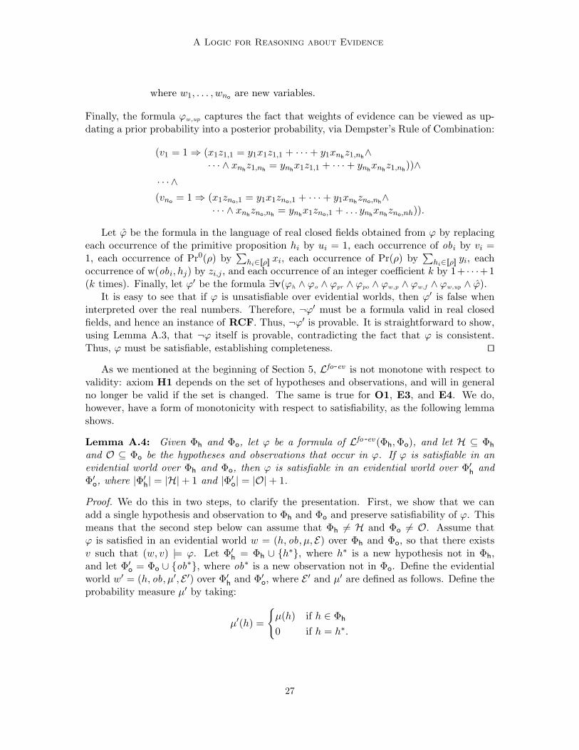
A Logic for Reasoning about Evidence
where w1, . . . , wno are new variables.
Finally, the formula ϕw,up captures the fact that weights of evidence can be viewed as up-dating a prior probability into a posterior probability, via Dempster’s Rule of Combination:
(v1 = 1 ⇒ (x1z1,1 = y1x1z1,1 + · · ·+ y1xnhz1,nh
∧· · · ∧ xnh
z1,nh= ynh
x1z1,1 + · · ·+ ynhxnh
z1,nh))∧
· · · ∧(vno = 1 ⇒ (x1zno,1 = y1x1zno,1 + · · ·+ y1xnh
zno,nh∧
· · · ∧ xnhzno,nh
= ynhx1zno,1 + . . . ynh
xnhzno,nh)).
Let ϕ̂ be the formula in the language of real closed fields obtained from ϕ by replacingeach occurrence of the primitive proposition hi by ui = 1, each occurrence of obi by vi =1, each occurrence of Pr0(ρ) by
∑hi∈[[ρ]] xi, each occurrence of Pr(ρ) by
∑hi∈[[ρ]] yi, each
occurrence of w(obi, hj) by zi,j , and each occurrence of an integer coefficient k by 1+ · · ·+1(k times). Finally, let ϕ′ be the formula ∃v(ϕh ∧ ϕo ∧ ϕpr ∧ ϕpo ∧ ϕw,p ∧ ϕw,f ∧ ϕw,up ∧ ϕ̂).
It is easy to see that if ϕ is unsatisfiable over evidential worlds, then ϕ′ is false wheninterpreted over the real numbers. Therefore, ¬ϕ′ must be a formula valid in real closedfields, and hence an instance of RCF. Thus, ¬ϕ′ is provable. It is straightforward to show,using Lemma A.3, that ¬ϕ itself is provable, contradicting the fact that ϕ is consistent.Thus, ϕ must be satisfiable, establishing completeness. ut
As we mentioned at the beginning of Section 5, Lfo-ev is not monotone with respect tovalidity: axiom H1 depends on the set of hypotheses and observations, and will in generalno longer be valid if the set is changed. The same is true for O1, E3, and E4. We do,however, have a form of monotonicity with respect to satisfiability, as the following lemmashows.
Lemma A.4: Given Φh and Φo, let ϕ be a formula of Lfo-ev (Φh,Φo), and let H ⊆ Φh
and O ⊆ Φo be the hypotheses and observations that occur in ϕ. If ϕ is satisfiable in anevidential world over Φh and Φo, then ϕ is satisfiable in an evidential world over Φ′
h andΦ′
o, where |Φ′h| = |H|+ 1 and |Φ′
o| = |O|+ 1.
Proof. We do this in two steps, to clarify the presentation. First, we show that we canadd a single hypothesis and observation to Φh and Φo and preserve satisfiability of ϕ. Thismeans that the second step below can assume that Φh 6= H and Φo 6= O. Assume thatϕ is satisfied in an evidential world w = (h, ob, µ, E) over Φh and Φo, so that there existsv such that (w, v) |= ϕ. Let Φ′
h = Φh ∪ {h∗}, where h∗ is a new hypothesis not in Φh,and let Φ′
o = Φo ∪ {ob∗}, where ob∗ is a new observation not in Φo. Define the evidentialworld w′ = (h, ob, µ′, E ′) over Φ′
h and Φ′o, where E ′ and µ′ are defined as follows. Define the
probability measure µ′ by taking:
µ′(h) =
{µ(h) if h ∈ Φh
0 if h = h∗.
27

Halpern & Pucella
Similarly, define the evidence space E ′ = (Φ′h,Φ
′o,µ
′) derived from E = (Φh,Φo,µ) by taking:
µ′h(ob) =
µh(ob) if h ∈ Φh and ob ∈ Φo
0 if h ∈ Φh and ob = ob∗
0 if h = h∗ and ob ∈ Φo
1 if h = h∗ and ob ∈ ob∗.
Thus, µ′h extends the existing µh by assigning a probability of 0 to the new observation ob∗;in contrast, the new probability µ′h∗ assigns probability 1 to the new observation ob∗. Wecan check that (w′, v) |= ϕ.
The second step is to “collapse” all the hypotheses and observations that do not appearin ϕ into one of the hypotheses that do not appear in H and O, which by the previous stepare guaranteed to exist. By the previous step, we can assume that Φh 6= H and Φo 6= O.Assume ϕ is satisfiable in an evidential world w = (h, ob, µ, E) over Φh and Φo, that is,there exists v such that (w, v) |= ϕ. Pick an hypothesis and an observation from Φh and Φo
as follows, depending on the hypothesis h and observation ob in w. Let h† be h if h 6∈ H,otherwise, let h† be an arbitrary element of Φh −H; let Φ′
h = H ∪ {h†}. Similarly, let ob†
be ob if ob 6∈ O, otherwise, let ob† be an arbitrary element of Φo −O; let Φ′o = O ∪ {ob†}.
Let w′ = (h, ob, µ′, E ′) be an evidential world over Φ′h and Φ′
o obtained from w as follows.Define the probability measure µ′ by taking:
µ′(h) =
{µ(h) if h ∈ H∑
h′∈Φh−H µ(h′) if h = h†.
Define E ′ = (Φ′h,Φ
′o,µ
′) derived from E = (Φh,Φo,µ) by taking:
µ′h(ob) =
µh(ob) if h ∈ H and ob ∈ O∑
ob′∈Φo−O µh(ob ′) if h ∈ H and ob = ob†∑h′∈Φh−H µh′(ob) if h = h† and ob ∈ O∑h′∈Φh−H
∑ob′∈Φo−O µh′(ob ′) if h = h† and ob = ob†.
We can check by induction that (w′, v) |= ϕ. ut
Theorem 5.1: There is a procedure that runs in space exponential in |ϕ| ‖ϕ‖ for deciding,given Φh and Φo, whether a formula ϕ of Lfo-ev (Φh,Φo) is satisfiable in an evidential world.
Proof. Let ϕ be a formula of Lfo-ev (Φh,Φo). By Lemma A.4, ϕ is satisfiable if we canconstruct a probability measure µ on Φ′
h = H ∪ {h∗} (where H is the set of hypothesesappearing in ϕ, and h∗ 6∈ H) and probability measures µh1 , . . . , µhm on Φ′
o = O ∪ {ob∗}(where O is the set of observations appearing in ϕ and ob∗ 6∈ O) such that E = (Φ′
h,Φ′o,µ),
w = (h, ob, µ, E) with (w, v) |= ϕ for some h, ob, and v.The aim now is to derive a formula ϕ′ in the language of real closed fields that asserts
the existence of these probability measures. More precisely, we can adapt the constructionof the formula ϕ′ from ϕ in the proof of Theorem 4.1. The one change we need to makeis ensure that ϕ′ is polynomial in the size of ϕ, which the construction in the proof of
28
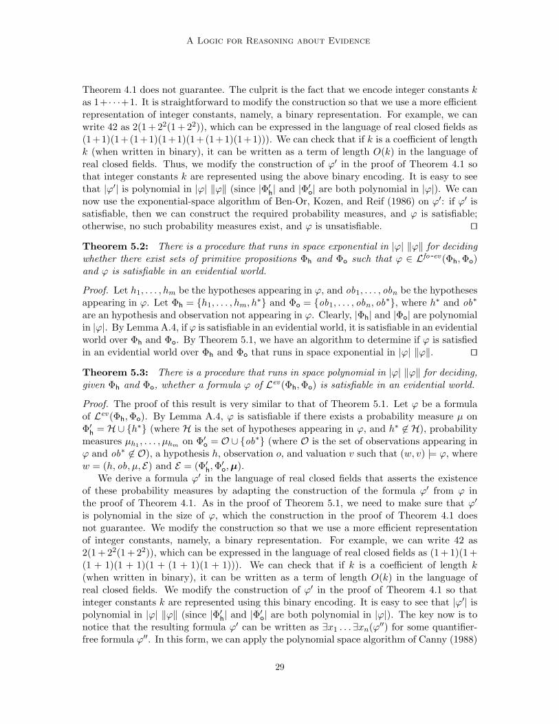
A Logic for Reasoning about Evidence
Theorem 4.1 does not guarantee. The culprit is the fact that we encode integer constants kas 1+ · · ·+1. It is straightforward to modify the construction so that we use a more efficientrepresentation of integer constants, namely, a binary representation. For example, we canwrite 42 as 2(1 + 22(1 + 22)), which can be expressed in the language of real closed fields as(1+1)(1+(1+1)(1+1)(1+(1+1)(1+1))). We can check that if k is a coefficient of lengthk (when written in binary), it can be written as a term of length O(k) in the language ofreal closed fields. Thus, we modify the construction of ϕ′ in the proof of Theorem 4.1 sothat integer constants k are represented using the above binary encoding. It is easy to seethat |ϕ′| is polynomial in |ϕ| ‖ϕ‖ (since |Φ′
h| and |Φ′o| are both polynomial in |ϕ|). We can
now use the exponential-space algorithm of Ben-Or, Kozen, and Reif (1986) on ϕ′: if ϕ′ issatisfiable, then we can construct the required probability measures, and ϕ is satisfiable;otherwise, no such probability measures exist, and ϕ is unsatisfiable. ut
Theorem 5.2: There is a procedure that runs in space exponential in |ϕ| ‖ϕ‖ for decidingwhether there exist sets of primitive propositions Φh and Φo such that ϕ ∈ Lfo-ev (Φh,Φo)and ϕ is satisfiable in an evidential world.
Proof. Let h1, . . . , hm be the hypotheses appearing in ϕ, and ob1, . . . , obn be the hypothesesappearing in ϕ. Let Φh = {h1, . . . , hm, h
∗} and Φo = {ob1, . . . , obn, ob∗}, where h∗ and ob∗
are an hypothesis and observation not appearing in ϕ. Clearly, |Φh| and |Φo| are polynomialin |ϕ|. By Lemma A.4, if ϕ is satisfiable in an evidential world, it is satisfiable in an evidentialworld over Φh and Φo. By Theorem 5.1, we have an algorithm to determine if ϕ is satisfiedin an evidential world over Φh and Φo that runs in space exponential in |ϕ| ‖ϕ‖. ut
Theorem 5.3: There is a procedure that runs in space polynomial in |ϕ| ‖ϕ‖ for deciding,given Φh and Φo, whether a formula ϕ of Lev (Φh,Φo) is satisfiable in an evidential world.
Proof. The proof of this result is very similar to that of Theorem 5.1. Let ϕ be a formulaof Lev (Φh,Φo). By Lemma A.4, ϕ is satisfiable if there exists a probability measure µ onΦ′
h = H∪ {h∗} (where H is the set of hypotheses appearing in ϕ, and h∗ 6∈ H), probabilitymeasures µh1 , . . . , µhm on Φ′
o = O ∪ {ob∗} (where O is the set of observations appearing inϕ and ob∗ 6∈ O), a hypothesis h, observation o, and valuation v such that (w, v) |= ϕ, wherew = (h, ob, µ, E) and E = (Φ′
h,Φ′o,µ).
We derive a formula ϕ′ in the language of real closed fields that asserts the existenceof these probability measures by adapting the construction of the formula ϕ′ from ϕ inthe proof of Theorem 4.1. As in the proof of Theorem 5.1, we need to make sure that ϕ′
is polynomial in the size of ϕ, which the construction in the proof of Theorem 4.1 doesnot guarantee. We modify the construction so that we use a more efficient representationof integer constants, namely, a binary representation. For example, we can write 42 as2(1 + 22(1 + 22)), which can be expressed in the language of real closed fields as (1 + 1)(1 +(1 + 1)(1 + 1)(1 + (1 + 1)(1 + 1))). We can check that if k is a coefficient of length k(when written in binary), it can be written as a term of length O(k) in the language ofreal closed fields. We modify the construction of ϕ′ in the proof of Theorem 4.1 so thatinteger constants k are represented using this binary encoding. It is easy to see that |ϕ′| ispolynomial in |ϕ| ‖ϕ‖ (since |Φ′
h| and |Φ′o| are both polynomial in |ϕ|). The key now is to
notice that the resulting formula ϕ′ can be written as ∃x1 . . .∃xn(ϕ′′) for some quantifier-free formula ϕ′′. In this form, we can apply the polynomial space algorithm of Canny (1988)
29

Halpern & Pucella
to ϕ′′: if ϕ′′ is satisfiable, then we can construct the required probability measures, and ϕis satisfiable; otherwise, no such probability measures exist, and ϕ is unsatisfiable. ut
Theorem 5.4: There is a procedure that runs in space polynomial in |ϕ| ‖ϕ‖ for decidingwhether there exists sets of primitive propositions Φh and Φo such that ϕ ∈ Lev (Φh,Φo) andϕ is satisfiable in an evidential world.
Proof. Let h1, . . . , hm be the hypotheses appearing in ϕ, and ob1, . . . , obn be the hypothesesappearing in ϕ. Let Φh = {h1, . . . , hm, h
∗} and Φo = {ob1, . . . , obn, ob∗}, where h∗ and ob∗
are an hypothesis and observation not appearing in ϕ. Clearly, |Φh| and |Φo| are polynomialin |ϕ|. By Lemma A.4, if ϕ is satisfiable in an evidential world, it is satisfiable in an evidentialworld over Φh and Φo. By Theorem 5.3, we have an algorithm to determine if ϕ is satisfiedin an evidential world over Φh and Φo that runs in space polynomial in |ϕ| ‖ϕ‖. ut
The proofs of Theorem 6.1 and 6.2 rely on the following small model result, a variationon Lemma A.4.
Lemma A.5: Given Φh and Φo, let ϕ be a formula of Lfo-ev (Φh,Φo), and let H ⊆ Φh
and O ⊆ Φo be the hypotheses and observations that occur in ϕ. If ϕ is satisfiable in anevidential world over Φh and Φo, then ϕ is satisfiable in an evidential world over Φ′
h andΦ′
o where |Φ′h| = |H|+ 1 and |Φ′
o| = |O|+ 1, and where, for each h ∈ Φ′h and ob ∈ Φ′
o, thelikelihood µh(ob) is a rational number with size O(|ϕ| ‖ϕ‖+ |ϕ| log(|ϕ|)).
Proof. Let ϕ be a formula satisfiable in an evidential world over Φh and Φo. By Lemma A.4,ϕ is satisfiable in an evidential world over Φ′
h and Φ′o, where |Φ′
h| = |H|+1 and |Φ′o| = |O|+1.
To force the likelihoods to be small, we adapt Theorem 2.6 in FHM, which says thatif a formula f in the FHM logic is satisfiable, it is satisfiable in a structure where theprobability assigned to each state of the structure is a rational number with size O(|f | ‖f‖+|f | log(|f |)). The formulas in Lw (Φ′
h,Φ′o) are just formulas in the FHM logic. The result
adapts immediately, and yields the required bounds for the size of the likelihoods. ut
Theorem 6.1: The problem of deciding, given Φh and Φo, whether a formula ϕ of Lw (Φh,Φo)is satisfiable in an evidential world is NP-complete.
Proof. To establish the lower bound, observe that we can reduce propositional satisfiabilityto satisfiability in Lw (Φh,Φo). More precisely, let f be a propositional formula, wherep1, . . . , pn are the primitive propositions appearing in f . Let Φo = {ob1, . . . , obn, ob∗} bea set of observations, where observation obi corresponds to the primitive proposition pi,and ob∗ is another (distinct) observation; let Φh be an arbitrary set of hypotheses, and leth be an arbitrary hypothesis in Φh. Consider the formula f̂ obtained by replacing everyoccurrence of pi in f by w(obi, h) > 0. It is straightforward to verify that f is satisfiableif and only if f̂ is satisfiable in Lw (Φh,Φo). (We need the extra observation ob∗ to takecare of the case f is satisfiable in a a model where each of p1, . . . , pn is false. In that case,w(ob1, h) = · · ·w(obn, h) = 0, but we can take w(ob∗, h) = 1.) This establishes the lowerbound,
The upper bound is straightforward. By Lemma A.5, an evidential world over Φh andΦo can be guessed in time polynomial in |Φh| + |Φo| + |ϕ| ‖ϕ‖, since the prior probabilityin the world requires assigning a value to |Φh| hypotheses, and the evidence space requires
30

A Logic for Reasoning about Evidence
|Φh| likelihood functions, each assigning a value to |Φo| observations, of size polynomial in|ϕ| ‖ϕ‖. We can verify that a world satisfies ϕ in time polynomial in |ϕ| ‖ϕ‖+ |Φh|+ |Φh|.This establishes that the problem is in NP. ut
Theorem 6.2: The problem of deciding, for a formula ϕ, whether there exists sets ofprimitive propositions Φh and Φo such that ϕ ∈ Lw (Φh,Φo) and ϕ is satisfiable in anevidential world is NP-complete.
Proof. For the lower bound, we reduce from the decision problem of Lw (Φh,Φo) over fixedΦh and Φo. Let Φh = {h1, . . . , hm} and Φo = {ob1, . . . , obn}, and let ϕ be a formula inLw (Φh,Φo). We can check that ϕ is satisfiable in evidential world over Φh and Φo if andonly if ϕ∧(h1∨· · ·∨hm)∧(ob1∨· · ·∨obn) is satisfiable in an evidential world over arbitraryΦ′
h and Φ′o. Thus, by Theorem 6.1, we get our lower bound.
For the upper bound, by Lemma A.5, if ϕ is satisfiable, it is satisfiable in an evidentialworld over Φh and Φo, where Φh = H∪ {h∗}, H consists of the hypotheses appearing in ϕ,Φo = O ∪ {ob∗}, O consists of the observations appearing in ϕ, and h∗ and ob∗ are newhypotheses and observations. Thus, |Φh| ≤ |ϕ| + 1, and |Φo| ≤ |ϕ| + 1. As in the proof ofTheorem 6.1, such a world can be guessed in time polynomial in |ϕ| ‖ϕ‖+ |Φh|+ |Φo|, andtherefore in time polynomial in |ϕ| ‖ϕ‖. We can verify that this world satisfies ϕ in timepolynomial in |ϕ| ‖ϕ‖, establishing that the problem is in NP. ut
Theorem 7.1: AXdyn(Φh,Φo) is a sound and complete axiomatization for Lfo-evdyn (Φh,Φo)
with respect to evidential runs.
Proof. It is easy to see that each axiom is valid in evidential runs. To prove completeness, wefollow the same procedure as in the proof of Theorem 4.1, showing that if ϕ is consistent,then it is satisfiable, that is, there exists an evidential run r and valuation v such that(r,m, v) |= ϕ for some point (r,m) of r.
As in the body of the paper, let Φh = {h1, . . . , hnh} and Φo = {ob1, . . . , obno}. Let ϕ be
a consistent formula. The first step of the process is to reduce the formula ϕ to a canonicalform with respect to the © operator. Intuitively, we push down every occurrence of a © tothe polynomial inequality formulas present in the formula. It is easy to see that axioms andinference rules T1–T6 can be used to establish that ϕ is provably equivalent to a formulaϕ′ where every occurrence of © is in the form of subformulas ©n(ob) and ©n(p ≥ c), wherep is a polynomial term that contains at least one occurrence of the Pr operator. We use thenotation ©nϕ for © . . .©ϕ, the n-fold application of © to ϕ. We write ©0ϕ for ϕ. Let Nbe the maximum coefficient of © in ϕ′.
By way of contradiction, assume that ϕ′ (and hence ϕ) is unsatisfiable. As in the proofof Theorem 4.1, we reduce the formula ϕ′ to an equivalent formula in the language of realclosed fields. Let u1, . . . , unh
, v01, . . . , v
0no, . . . , vN
1 , . . . , vNno
, y01, . . . , y
0no, . . . , yN
1 , . . . , yNno
, andz〈i1,...,ik〉,1, . . . , z〈i1,...,ik〉,nh
(for every sequence 〈i1, . . . , ik〉) be new variables, where, intu-itively,
• ui gets value 1 if hypothesis hi holds, 0 otherwise;
• vni gets value 1 if observation obi holds at time n, 0 otherwise;
• yni represents Pr(hi) at time n;
31
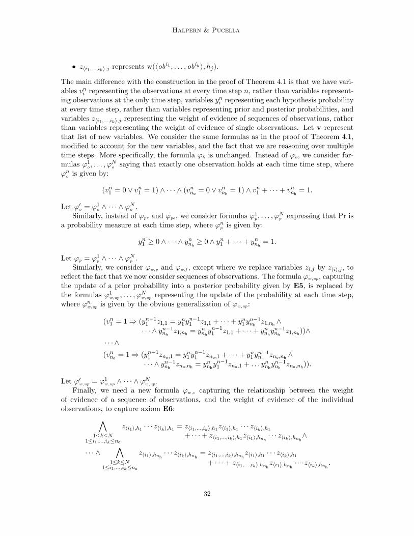
Halpern & Pucella
• z〈i1,...,ik〉,j represents w(〈obi1 , . . . , obik〉, hj).
The main difference with the construction in the proof of Theorem 4.1 is that we have vari-ables vn
i representing the observations at every time step n, rather than variables represent-ing observations at the only time step, variables yn
i representing each hypothesis probabilityat every time step, rather than variables representing prior and posterior probabilities, andvariables z〈i1,...,ik〉,j representing the weight of evidence of sequences of observations, ratherthan variables representing the weight of evidence of single observations. Let v representthat list of new variables. We consider the same formulas as in the proof of Theorem 4.1,modified to account for the new variables, and the fact that we are reasoning over multipletime steps. More specifically, the formula ϕh is unchanged. Instead of ϕo, we consider for-mulas ϕ1
o , . . . , ϕNo saying that exactly one observation holds at each time time step, where
ϕno is given by:
(vn1 = 0 ∨ vn
1 = 1) ∧ · · · ∧ (vnno
= 0 ∨ vnnh
= 1) ∧ vn1 + · · ·+ vn
nh= 1.
Let ϕ′o = ϕ1o ∧ · · · ∧ ϕN
o .Similarly, instead of ϕpr and ϕpo, we consider formulas ϕ1
p , . . . , ϕNp expressing that Pr is
a probability measure at each time step, where ϕnp is given by:
yn1 ≥ 0 ∧ · · · ∧ yn
nh≥ 0 ∧ yn
1 + · · ·+ ynnh
= 1.
Let ϕp = ϕ1p ∧ · · · ∧ ϕN
p .Similarly, we consider ϕw,p and ϕw,f , except where we replace variables zi,j by z〈i〉,j , to
reflect the fact that we now consider sequences of observations. The formula ϕw,up, capturingthe update of a prior probability into a posterior probability given by E5, is replaced bythe formulas ϕ1
w,up, . . . , ϕNw,up representing the update of the probability at each time step,
where ϕnw,up is given by the obvious generalization of ϕw,up:
(vn1 = 1 ⇒ (yn−1
1 z1,1 = yn1 y
n−11 z1,1 + · · ·+ yn
1 yn−1nh
z1,nh∧
· · · ∧ yn−1nh
z1,nh= yn
nhyn−11 z1,1 + · · ·+ yn
nhyn−1
nhz1,nh
))∧· · · ∧(vn
no= 1 ⇒ (yn−1
1 zno,1 = yn1 y
n−11 zno,1 + · · ·+ yn
1 yn−1nh
zno,nh∧
· · · ∧ yn−1nh
zno,nh= yn
nhyn−11 zno,1 + . . . yn
nhyn−1
nhzno,nh
)).
Let ϕ′w,up = ϕ1w,up ∧ · · · ∧ ϕN
w,up.Finally, we need a new formula ϕw,c capturing the relationship between the weight
of evidence of a sequence of observations, and the weight of evidence of the individualobservations, to capture axiom E6:∧
1≤k≤N1≤i1,...,ik≤no
z〈i1〉,h1· · · z〈ik〉,h1
= z〈i1,...,ik〉,h1z〈i1〉,h1
· · · z〈ik〉,h1
+ · · ·+ z〈i1,...,ik〉,h1z〈i1〉,hnh
· · · z〈ik〉,hnh∧
· · · ∧∧
1≤k≤N1≤i1,...,ik≤no
z〈i1〉,hnh· · · z〈ik〉,hnh
= z〈i1,...,ik〉,hnhz〈i1〉,h1
· · · z〈ik〉,h1
+ · · ·+ z〈i1,...,ik〉,hnhz〈i1〉,hnh
· · · z〈ik〉,hnh.
32

A Logic for Reasoning about Evidence
Let ϕ̂ be the formula in the language of real closed fields obtained from ϕ by replacingeach occurrence of the primitive proposition hi by ui = 1, each occurrence of ©nobi byvni = 1, and within each polynomial inequality formula ©n(p ≥ c), replacing each occurrence
of Pr(ρ) by∑
hi∈[[ρ]] yni , each occurrence of w(〈obi1 , . . . , obik〉, hj) by z〈i1,...,ik〉,j , and each
occurrence of an integer coefficient k by 1 + · · ·+ 1 (k times). Finally, let ϕ′ be the formula∃v(ϕh ∧ ϕ′o ∧ ϕp ∧ ϕw,p ∧ ϕw,f ∧ ϕ′w,up ∧ ϕw,c ∧ ϕ̂).
It is easy to see that if ϕ is unsatisfiable over evidential systems, then ϕ′ is false aboutthe real numbers. Therefore, ¬ϕ′ must be a formula valid in real closed fields, and hence aninstance of RCF. Thus, ¬ϕ′ is provable. It is straightforward to show, using the obviousvariant of Lemma A.3 that ¬ϕ itself is provable, contradicting the fact that ϕ is consistent.Thus, ϕ must be satisfiable, establishing completeness. ut
References
Ben-Or, M., Kozen, D., & Reif, J. H. (1986). The complexity of elementary algebra andgeometry. Journal of Computer and System Sciences, 32 (1), 251–264.
Canny, J. F. (1988). Some algebraic and geometric computations in PSPACE. In Proc. 20thAnnual ACM Symposium on the Theory of Computing (STOC’88), pp. 460–467.
Carnap, R. (1962). Logical Foundations of Probability (Second edition). University ofChicago Press.
Casella, G., & Berger, R. L. (2001). Statistical Inference (Second edition). Duxbury.
Chan, H., & Darwiche, A. (2005). On the revision of probabilistic beliefs using uncertainevidence. Artificial Intelligence, 163, 67–90.
de Alfaro, L. (1998). Formal Verification of Probabilistic Systems. Ph.D. thesis, StanfordUniversity. Available as Technical Report STAN-CS-TR-98-1601.
Enderton, H. B. (1972). A Mathematical Introduction to Logic. Academic Press.
Fagin, R., & Halpern, J. Y. (1994). Reasoning about knowledge and probability. Journalof the ACM, 41 (2), 340–367.
Fagin, R., Halpern, J. Y., & Megiddo, N. (1990). A logic for reasoning about probabilities.Information and Computation, 87 (1/2), 78–128.
Fischer, M. J., & Zuck, L. D. (1988). Reasoning about uncertainty in fault-tolerant dis-tributed systems. Technical report YALEU/DCS/TR–643, Yale University.
Good, I. J. (1950). Probability and the Weighing of Evidence. Charles Griffin & Co. Ltd.
Good, I. J. (1960). Weights of evidence, corroboration, explanatory power, informationand the utility of experiments. Journal of the Royal Statistical Society, Series B, 22,319–331.
Halpern, J. Y., & Fagin, R. (1992). Two views of belief: belief as generalized probabilityand belief as evidence. Artificial Intelligence, 54, 275–317.
33

Halpern & Pucella
Halpern, J. Y., Moses, Y., & Tuttle, M. R. (1988). A knowledge-based analysis of zeroknowledge. In Proc. 20th Annual ACM Symposium on the Theory of Computing(STOC’88), pp. 132–147.
Halpern, J. Y., & Pucella, R. (2003). A logic for reasoning about evidence. In Proc. 19thConference on Uncertainty in Artificial Intelligence (UAI’03), pp. 297–304.
Halpern, J. Y., & Pucella, R. (2005a). Evidence with uncertain likelihoods. In Proc. 21thConference on Uncertainty in Artificial Intelligence (UAI’05), pp. 243–250.
Halpern, J. Y., & Pucella, R. (2005b). Probabilistic algorithmic knowledge. Logical Methodsin Computer Science, 1 (3:1).
Halpern, J. Y., & Tuttle, M. R. (1993). Knowledge, probability, and adversaries. Journalof the ACM, 40 (4), 917–962.
He, J., Seidel, K., & McIver, A. (1997). Probabilistic models for the guarded commandlanguage. Science of Computer Programming, 28 (2–3), 171–192.
Jeffrey, R. C. (1992). Probability and the Art of Judgement. Cambridge University Press.
Kyburg, Jr., H. E. (1983). Recent work in inductive logic. In Machan, T., & Lucey, K.(Eds.), Recent Work in Philosophy, pp. 87–150. Rowman & Allanheld.
Milne, P. (1996). log[p(h|eb)/p(h|b)] is the one true measure of confirmation. Philosophy ofScience, 63, 21–26.
Pearl, J. (1988). Probabilistic Reasoning in Intelligent Systems: Networks of PlausibleInference. Morgan Kaufmann.
Popper, K. R. (1959). The Logic of Scientific Discovery. Hutchinson.
Renegar, J. (1992). On the computational complexity and geometry of the first order theoryof the reals. Journal of Symbolic Computation, 13 (3), 255–352.
Shafer, G. (1976). A Mathematical Theory of Evidence. Princeton University Press.
Shafer, G. (1982). Belief functions and parametric models (with commentary). Journal ofthe Royal Statistical Society, Series B, 44, 322–352.
Shoenfield, J. R. (1967). Mathematical Logic. Addison-Wesley, Reading, Mass.
Tarski, A. (1951). A Decision Method for Elementary Algebra and Geometry (2nd edition).Univ. of California Press.
Vardi, M. Y. (1985). Automatic verification of probabilistic concurrent finite-state programs.In Proc. 26th IEEE Symposium on the Foundations of Computer Science (FOCS’85),pp. 327–338.
Walley, P. (1987). Belief function representations of statistical evidence. Annals of Statistics,18 (4), 1439–1465.
34