A Local Theory of Input/Output Stability of Dynamical Systems

by H O R A C I O MARQUEZ~"

Department o f Enyineering, Royal Roads Military College, F M O Victoria, British Columbia, VOS 1BO, Canada

ABSTRACT : The purpose of this paper is to present a local theory of input/output stability OJ dynamical systems. More precisely, the intention is to obtain local open loop conditions for local closed loop stability of feedback interconnections. It will be shown that, by setting the problem in the context of extended binormed spaces it is possible to obtain local versions of the so-called small 9ain theorem and circle criterion for stability of nonlinear systems. The results clearly determine the extent of input~output stability, i.e. the set of input.[hnctions./br which stability is 9uaranteed.

L Introduction

In this paper we are concerned with stability of dynamical systems. Roughly speaking, there are two conceptually different approaches to stability theory: (i) Lyapunov theory, and (ii) the input/output approach. The former studies the stability of an equilibrium state of the autonomous, or unforced system, while the latter regards systems as mappinys between inputs and outputs. The Lyapunov theory was initiated by A. M. Lyapunov in the 1890s and it is summarized in several textbooks [see for example (1-3)], while the input/output theory was initiated in the 1960s by G. Zames (4, 5), and I. Sandberg (6, 7). See also references (8, 9) for thorough expositions of the input/output theory. Intrinsic in the philosophical differences between these two approaches is the fact that, while the Lyapunov theory is essentially local, i.e. the definition of stability is assumed to hold in some small region about an equilibrium point, the input/output theory is global, i.e. systems are said to be stable if the system output belongs to some space of functions whenever the input belongs to the same space. This notion of stability is therefore 'global', in the sense that inputs and outputs can be any function within the prescribed space. In principle, it is straightforward to formulate a local definition of input/output stability. To do so one simply has to restrict the input signals to some subset of the space of functions. However, the main aim of the input/output theory is the derivation of open loop conditions for stability of feedback inter- connections. Therefore, in general, such a definition would be futile in this context, unless the subset of the space of functions is defined in a way that can be used to obtain stability results for feedback systems.

I Visiting Fellow in a Canadian Government Laboratory.

~3 The Franklin Institute 001(~0032/95 $9.50+0.00 0016-0032(95)00035~, 9 l Pergamon

H. Marquez

The purpose of this article is to present a local input/output theory of dynamical systems. The importance of such a theory relies on the fact that many systems can be rendered input~output stable provided that the size of the input signals is kept small, in a sense to be defined, while the same is not true according to the classical notion of input/output stability. We depart from a new formulation of input/output stability, and generate local versions of the celebrated small gain theorem, and circle criteria for stability of a class of nonlinear systems.

II. Definitions In this section we lay down the mathematical basis for the theory of local

input/output stability. The main difference between the tools used in the classical (global) theory of input/output systems and the present one is that while the former is based on the use of normed linear spaces and their extension, the later will require the concept of extended binormed linear space. Define the following notation:

IR Field of real numbers + Set of nonnegative real numbers

A linear space f The space of functions x : ~ ~ ~ .

We will denote by (')v the truncation operator defined as follows: Given x e X, we define the function xr (') by

xr ( t )={ ; ( t ) i f t<~T i f t > T.

The extension of the space X, denoted f , . is defined to be the space of all functions whose truncation belongs to f .

The notion of binormed linear space will play a crucial role in the present theory. The following definition introduces this concept.

Definition 1 A binormed linear space is a triplet (~ , II'll~, II ' /I .) consistent of a linear space

~( over the field F, and two functions I1"11~, and/1"11,, : ~ --' ~+ such that

(i) [Ix[Io = 0 if and only i f x = 0 (i i) II,~xHo = 12111xll° V2EF, Vx~ f

(i i i) I Ix+y l lo ~< I lx l lo+ IlYlI° Vx, y 6 X , where a = ~e or ~¢" in ( i ) -( i i i ) . The functions I1"11~ and I I ' l l . wil l be referred to as the primary and secondary norms of the space ~e. In the sequel we will assume that F is the field IR of real numbers.

We will make the following assumptions regarding the space X :

(i) X is a binormed space, with primary and secondary norms I1"11.~, and II'll,~, respectively.

(ii) X is closed under the family of truncations {(')r}. In other words, if x e X, then X T ~ f , VT~ ~.

(iii) I f x 6 f , and T~ ~, then [[XT[[U" <~ I[XI[:7", and [IXT[I,~ ~< [Ixll... (iv) If x~Xe, then x ~ X if and only if l imv~llxr[[e- < ~ , and limr~l]xr[},

< 0 0 .

~ A Journal of the Franklin Institute 9 2 Elsevier Science Ltd

Input~Output Stability

In the sequel we will need to consider subsets of the set 5re, having some special properties.

Definition 2 Consider the space 5re. We define the subset ~WQ c 5f as follows :

~ ; -- { x ~ f : Ilxll,~-< Q}. (1)

In other words, ~ is the subset of f e consisting of functions whose secondary norm is less than Q e ~+. Notice that, while ~e is a linear space, ~//o is simply a balanced set. It is not a linear space since there exist elements x, y e ~ such that x + y ¢ ~ . The set ~¢/Q is balanced since given x e ~/~Q, then clearly 2x e ~FQ whenever 2E~, 121 ~ 1.

Definition 3 A system, or more precisely, the mathematical representation of a physical system,

is defined to be an operator H: 5re --+ Xe with the following properties :

(i) The zero element, denoted 0, lies in the domain of H, and moreover, H0 = 0. ( i i ) [Hx( ' ) ] T = [HXT(')]T, ~/X6,~{'e, VTe ~.

Condition (ii) of Definition 3 is a causality constraint, and simply states the fact, satisfied by all physical systems, that the past and present output do not depend on future inputs. We now state the definition of local stability. Notice that although we have assumed that systems are operators, the definition of local stability is stated using relations, a fact that will be useful in the proof of stability results. We recall that, given two nonempty sets A~ and A2, a relation ~ in Aj x A2 is any subset of the Cartesian product A j x A2. In other words, a relation is simply a correspondence law between the elements of two sets. We will denote by dom(~) and ran(~l) the domain and the range of ~ , respectively.

Definition 4 Let A~ and A2 be sets and consider the Cartesian product A, x A2. We will

denote by Pi, i = 1, 2 the function Pi: A1 x A2 ~ Ai, which carries each ordered pair of the form (Xl, x2) into its ith coordinates. That is, P~(x~, x2) = xz, i = 1, 2. The map Pi is called the evaluation map at i.

Definition 5 A relation ~ on 5re x Y'e is said to be ~(~-stable, or simply stable if the image of

the evaluation map at 2 is a bounded subset of Y'e whenever the image of the evaluation map at 1 belongs to the set "WQ. In other words, ~ is ~##Q-stable if ~ x e Y/', whenever x e ~ .

Remarks Definition 5 introduces the notion of ~WQ-stability. The closest concept en-

countered in the literature is that of 'small signal stability', introduced by Vidyasagar and Vannelli (see (10) Section 6.3) with the purpose of studying connections

Vol. 332B, No. 1, pp. 91 106, 1995 Printed in Great Britain. All rights reserved 93

H. Marquez

between the input/output and Lyapunov stability theories. Our formulation is however more general, and our objectives are different from those in (10).

We now define the notion of (open loop) input/output local stability.

Definition 6 Consider a system H: 5re ~ Y'e, and let Xo and Yo be such that Xo ~ dom(H) ,

yo~ran(H) , and (yo)T=(Hxo)r . We say that H is (input/output) locally stable about xo if the relation Jfoz, defined by

algol = { ( X - Xo, H x - Hxo) ~ e x 3Ye}, (2)

is ~¢@stable.

Remarks Notice that we do not assume that xo, x, Hx , and Hxo are in 5£. This is an

important feature of this formulation. Notice the contrast with the classical defi- nition of input/output stability, where a relation (or a system) is said to be stable if and only if the output is in the space 5f, whenever the input is in 5F. Our formulation is therefore more general and permits consideration of several cases of importance, not covered by the classical input/output theory. For example, many interesting stability results can be obtained using the space L2 (i.e. 5f,, = L2e). However, using the classical definition of input/output stability nothing can be said about the behaviour of the system driven by persistent inputs, such as steps, ramps, or sinusoids, since none of these signals are in L> It is important however to study what happens when a system, exited by one of these signals, is slightly perturbed, perhaps due to the effect of exogenous signals, such as noise or dis- turbances, superimposed to the persistent signal. The following straightforward example clarifies this point.

Example Let .~ = L2 ~ L~, and let IP'[[:~ = 1I"112 and P['[I,~ = 11"11~, where 11"112 and I['[[~ are

the usual L2 and L~o norms. Consider the system H: ~,, --, YFe defined by H = K, K~ ~, and let Yo be the output due to the unit step input, denoted u(t). In other words,

y o = K u ( t ) , u ( t ) = if t < 0 . (3)

We have

H x - Hx,, = Kx( t) - Ku( t) (4)

= K[x( t ) - u(t)]. (5)

Thus, H is locally stable about Xo = u(t), since H x - Hxo ~ ~? whenever ( x - Xo) ~ ~5.

Definition 7 Consider the system H: We -+ 5re (i.e. H is an operator satisfying the conditions

of Definition 3), and assume that H is locally stable about Xo. If there exist positive real numbers F~-(H, Xo), F~(H, Xo) < ~ such that

---- Journal of the Franklin Institute 9 4 Elsevier Science Ltd

Input~Output Stability

II (Hx) T-- (Hxo)~ll~ r~(H, xo) = sup IIXT--(Xo)~II~ '

V x such that [Xr - (Xo) r] e ~/¢~ c f , V T e ~ + (6)

II ( HX)T-- ( nXo)TIl,~ F , ( H , Xo) = sup IlXr-- (Xo)Tll~ '

V x such that [X T - (Xo)T] E % C ~f, ~/ Te R + (7)

then H is said to have local gains, F,~-(H, Xo), and F,~ (H, Xo).

The following lemma shows that the definition of local gain is not altered if all the truncations in the right hand side of Eqs (6) and (7) are dropped.

Lemma 1 Consider a system H: 2f,, -+ he,, and assume that there exists F*(H, x,,) e R + such

that

Il n x -- nxo ll,~- F*.(H, Xo) = sup IIx-xoll~, ' Vxsuchthat[x-x°]e~WQ' (8)

Then H has a finite local gain, and moreover, F*-(H, xo) = F.~.(H, x,,). A similar result can be obtained for the gain F,-(H, Xo).

Proof: We must show that

I[nx--nxolb. <<. F*.(n, xo)l[x-xoll..~., [ x - x o ] ~ o (9)

if and only if

II(Hx)r-(Hxo)yllJ. <~ F~(H, xo)llxy--(Xo)T[l:~, [ x r - ( X o ) r ] ~ o (10)

and moreover, F*(H,x,,) = E~.(H,x,,). Assume first that Eq. (10) holds. Thus if (x -x , , ) e "¢¢/Q, then ( x - x o ) T = X r-- (Xo)re ~¢/0, and we have

II ( H x ) r - (gxo)rH.~, <~ Ff (H, x, , ) f lxr- (xo)rll., (11)

and since (X -Xo )e ~¢/o, the last equation must also be satisfied when T ~ ~ . Therefore,

I l g x - Hxo[I,~- <. F.~.(H, Xo)llx- xoll:~.. (12)

It follows that

F:~.(H, xo) >~ F*-(H, xo). (13)

Assume now that Eq. (9) holds and consider x e~,. such that (x- -xo)e~Q. We have [X--Xo]T= [XT--(Xo)T]e~#/O, and then ]]HxT--H(xo)T]l <.F*.(H,x,,) Hxr-- (Xo)rH. But since H is causal,

[Hx-- Hxo] r = [Hx] T-- [HXo] r (14)

= [HXT]T-- [n(xo)r]r (15)

= [HxT-- H(xo)r]r (16)

and therefore

Vol. 332B, No. I, pp. 91 106, 1995 Printed in Great Britain. All rights reserved 95

H. Marquez

Thus,

II [Hx~- H(Xo)Tl~ll~ ~ I I H x r - H(xo)r[I.e ~

~< F*.(H, Xo)Ilxr- (Xo)TIl~.

r~-(H, xo) >7 F~.(H, Xo)

and the result follows by comparison of Eqs (13) and (19).

(17)

(18)

(19)

Remarks It is straightforward that if H is linear, then H is locally stable about Xo if and

only if H is locally stable about 0. Moreover, for linear systems the definitions of local and global gains are essentially equivalent. The following lemma summarizes these remarks.

Lemma 2 Let H: Y',, ~ Y'e be linear. Then,

(i) if H has local gains F~(H, Xo) and F , ( H , Xo) about Xo, then

r:~.(H, xo) = F.~.(H,0), r , ( H , xo) = F,~ (H,0).

(ii) the gains F:~.(H, Xo) and F, . (H, xo) are global, i.e. F~(H, 0) and F t ( H , 0) are valid for all x : ( x - Xo) e ~',,.

In view of these results, whenever we deal with linear systems we will write F.~-(H) and F~, (H) instead of K¢(H, Xo) and F~ (H, xo), respectively.

Proof o f Lemma 2 : For simplicity, we will write F(H, Xo) instead of F.~.(H, xo) or F,~.(H, Xo). Similarly, f1"11 represents either the primary or secondary norm of the space ~'.

To prove (i) :

F(H, xo) = sup

= sup

II Hx - Hxo H IIX-Xoll

V x such t h a t ( x - xo) e ~#/o

11 H(x - Xo)1] I lx - xo][ ' V x such t h a t ( x - xo) e #/~

Ilnzll

Journal of the Franklin Institute 9 0 Elsevier Science Ltd

= s u p s - , V z e ~ # @ z % f x - x o .

Thus, F(H, Xo) = F(H, 0). To prove (ii) : Let H have a local gain F(H, 0) for all x e ~#/Q. Then

IPHxll F(H, 0) = sup Ilxl[ ' V x ~ .

Consider now x ~ 5 c, x ¢ ~ , i.e. x is such that Ilxll~ < oc, Ilzll,,-- k > Q, and assume without loss of generality that Q > 1. It follows that z ~x/l lxl l ~ ~FQ, and then

but

and the result follows.

F(H, O) ~< sup

X

X

H ~ IIHxlb

Ilxll

Input~Output Stability

I lL Local Small Gain Conditions

In this section we consider feedback systems, and present a local version of the celebrated small gain theorem.

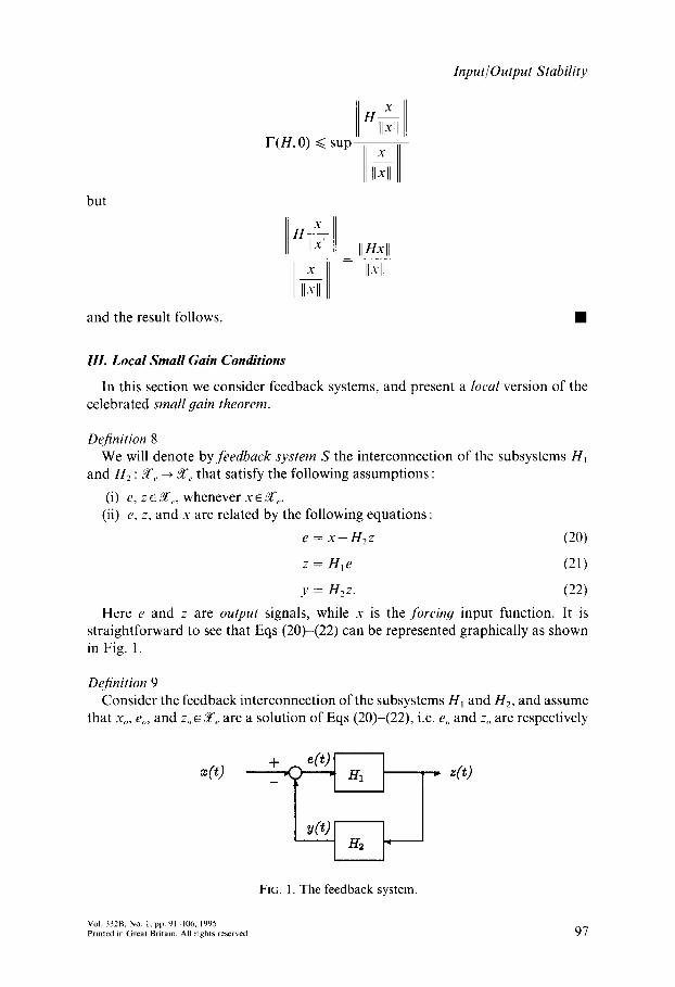
Definition 8 We will denote by feedback system S the interconnection of the subsystems H~

and H2 : ~,, ~ £ r that satisfy the following assumptions :

(i) e, z ~ ~',,, whenever x ~ ~e. (ii) e, z, and x are related by the following equations :

e = x - H2 z (20)

z = H i e (21)

y = H2z. (22)

Here e and z are output signals, while x is the forcing input function. It is straightforward to see that Eqs (20)-(22) can be represented graphically as shown in Fig. 1.

Definition 9 Consider the feedback interconnection of the subsystems H, and H2, and assume

that x,,, eo, and zo E f , , are a solution of Eqs (20)-(22), i.e. e, and Zo are respectively

FIG. 1. The feedback system.

Vol. 332B, No. 1, pp. 91 106, 1995 Printed in Grea! Britain. All rights reserved 97

H. Marquez

the error and the output of the feedback system of Fig. 1 when the external input is Xo. For this system define the following closed loop input-output relations: Given x ~ 5f,,, we define

o~,.t = {(X-Xo,e-eo)~Yfe×3f, .:x, esatisfyEqs(20)and(21)} (23)

~,., = {(x-xo, z -zo)~Y' , .xgf~:x , zsatisfyEqs(20) (22)}. (24)

In other words, g,.~ (respectively ~,.~) is the relation that relates the difference of the outputs e - e o (respectively z-Zo) to the difference of the inputs x -xo . Notice that dom(g,.~) and dom(Lrc~ ) are never empty since, by assumption, (xo-x,,, eo-e,,) and (Xo-Xo, Zo-zo) belong to dom(o~,.~) and dom(Lr,.t), respectively.

Definition 10 The feedback system of Eqs (20)-(22) is said to be locally stable about xo if the

relations g,.t and ~,.t are both ~ - s t ab le .

We now define the following special classes of systems.

Definition 11 H: ST,, ~ ~ e is said to be in the class cg,~ if there exist ~ and S e [~+ such that

II[nx~]r-[nx2]r]l~ <~ ~llxlr--X2r]l~, VX,: IlxiT--X0TII~ ~ S, i = 1,2.

This condition implies that H is Lipschitz continuous, with respect to the secondary norm I1" I1,~, for all x: ( X - X o ) ~ s . Notice also that this guarantees that if I Ix-x0 In ,~ is small enough, then In Hx--Hx0 II ~, < Q. In other words, local models in the class cg~ map ~ss into ~o, for some small enough S e ~+.

Definition 12 A system H: Y',,-~ Y£,, is said to be in the class ~ r if for each input x(t)~?t',,,

0 < I T - r l < 6 implies that

II[Hx]r-[Hx]~ll~ < ~, V x ~ ' , , .

In particular, notice that the assumptions made on the space 5re imply [Hx]0 = 0, V x ~ ~r. Thus we have

II[nx]T--[nx]oll~, = I][nx]TIl~ < ~, VxE~',,

provided that I TI < 6. In other words, H is in the class cgr if for each x(t) ~ Y'~, the output Hx(t) is ~¢/:

continuous with respect to the family of projections ( ' ) r . Notice the difference with the Lipschitz continuity condition of Definition 11. This class prevents con- sideration of certain ideal models of physical systems, such as for instance H = K (constant), which are indeed Lipschitz continuous in the sense of Definition 11, but where the output due to certain inputs can change instantaneously.

Theorem 1 Let HI, H2: ~,, ~ &re and consider the feedback system defined by Eqs (20)

(22). Assume that H1 ~ cgr, H2 e ~g,~, and suppose that when x = Xo the system admits a solution of the form

Journal of the Franklin Institute ~ Elsevier Science Lid

Input~Output Stability

eo = Xo - H z z o (25)

Zo = Hleo. (26)

Under these conditions, if the product of the local gains Fs-(H1, eo)Fj-(H2, zo) < 1, and F , (H i , eo)F~,(H2, Zo) < 1, then the system is closed loop stable about xo.

Proof: Truncating Eq. (20) and using the fact that HI and H~ are both causal, we have

er = XT-- [H2Zr]T

= XT--[H~_(Hler)T]T

and therefore

Thus

and

(eo)T = (Xo)T-- {H2[H, (e,,)r]r}r

eT ---- Xr-- [H2 (HI er)T] r

[er-- (eo) r] = [ X r - (Xo)T] + {H2 [H, (eo)T]r} T-- {H2 [H1 er]r} r.

IleT-(eo)Tll~ ~ I[XT--(Xo)TII.~+II{H2[H, eT]T}T--{H2[HI(eo)r]T}TI[~ (27)

IleT-- (eo)rH ~ ~ IIxT-- (Xo)TII ~ + II {H2[H, er]r}r-- {H2[H, (eo)r]r}rll ~. (28)

At t = 0 the system is at rest and so we have x ( 0 ) = 0 , e ( 0 ) = 0 , z(O) = (H~e)(O) = 0, and y(0) = (H2z)(0) = 0. Since H~ is in the class cgv, we have

[][Hler]r--[H, er]ol[~ = [l[HleT]rl[~ < e,

and

IIKH, e0v]r--[Hleor]o II,~ = II[Hleor]rl]~ < e2

provided that IT] < 5. Thus, we have

II[HleT]T--[HIeoT]Tllu <~ ~1 +e~_, VIT] < 6

and since H2 is Lipschitz continuous about Zor = Hj eov,

][[H2ZT]T--[H2ZoT]TI]~ <~ ~II[H, eT]T--[HIeoT]TH,

<~g(e1+g2)--e3, V l T I < 6 .

Thus, Eq. (28) implies that

[ler--e0Tll~ ~< ItXT--XoTII~+e3

and since (ev--eoT) ~.~re by assumption, it follows that ( e r - e 0 r ) e # o , for some Q = f ( T ) . Therefore, Eq. (28) implies that

I[er-(er)rll~ ~< [1-F~(Hl ,eo)F~(Hz,zo) ] l l lxr-(Xo)Tll , , . (29)

Therefore, the norm Her--(eo)rll,~ is bounded by the right hand side of (29). If in

Vol. 332B, No. I, pp. 91 106, 1995 Printed in Great Britain. All rights reserved 9 9

H. Marquez

addition ( x - xo) ~ fi/Q, we can take limits as T--* oo on both sides of (29), and we have

Ile-eoll,, ~< [1--F~(Hl ,Xo)F~.(H2,zo)]- ' IIx--xoll~. (30)

Thus, if IIx-xoll , , -< Q[1-F(Hi ,eo)F(H2,zo) ] , then (e-eo)e~/@ Similarly, it is easy to see that

IIzT--(Zo)T[I~ ~ F~(H, ,eo)[ l -Fu(H, ,eo)F~(H2,zo)] l l lx~-(xo)~ll~ (31)

and then, taking limits as T ~ ~ we conclude that if ]tx-xoll ,, < Q F , (HI, eo) [1 - F~ (H,, eo)Fu(H2, zo)], then (Z-Zo) ~ ~i¢/o. It follows that if

l l x - x o ] l ~

< min {Q[1 - F(HI, eo)F~ (H2, zo)], Q[F~ (H,, eo)] - '[1 - F,, (HI, e,,)F~ (H2, z,)]}

def Q . (32)

then (z-- zo) and ( e - eo) ~ ~/~e' We will denote by "#J~, the space of functions x ' I Ix-xol l~ < Q*. Thus, from Eq. (27), whenever x~Q*,

Iler--(eo)TII, <~ [ l -F~(H, ,eo)F.~(H2,zo)] I lIxT--(Xo)TII.~"

and taking limits as T ~ oe,

Ile-eoll.~. ~< [l-F.~.(Hi,eo)F~(H2,zo)] Ilrx--xoll~, IIx-xoll,, < Q*. (33)

In the same way

[Iz- zoll <~ F.o,(gl,eo)[1-r~-(H,,eo)r:,(H2,z,,)] ' t l x - xolF.,,

Thus, o~,,~ and ~ / a r e ~/¢/e stable, and the result follows.

IIx-xoll~ < Q*.

(34)

Remarks Theorem 1 presents a local version of the small gain theorem. It is important to

notice the crucial role played by the secondary norm, II'll ~. In particular, condition (32) defines the extent of local stability, i.e. the set of input functions for which stability is guaranteed.

IV. Local Circle Criteria and Extensions

In this section we study the stability of systems comprised of a linear time- invariant subsystem in the forward path and a memoryless nonlinearity in the feedback path. We will present a local version of the circle criterion, along with some extensions which naturally arise in some special cases.

Throughout this section we will make the following assumptions :

(i) ~ - - L 2 ~ L:~

(i i) [l'll:~ = 11°112 (iii) I1o11,, = 11"11~

Thus, ~ is the set of all functions x e L 2 c~ L~ such that Ilxll~ < Q.

Journal of the Franklin Institute 1 0 0 Elsevier Science Ltd

Input/Output Stability

We now define what is understood by a nonlinearity locally inside a sector.

Definition 13 A function d~: E + x ~ ~ ~ is said to be locally in the sector [~,/~] about x,, if it

satisfies

~(t, x) - ~ ( t , xo) <~ (x-Xo) <~ ~' Vt >t O, (x-x,,)~ #~, (x-xo) :g 0.

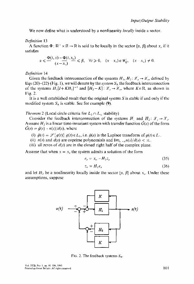
Definition 14 Given the feedback interconnection of the systems H~, H 2 : ~ 'e ~ ~'e, defined by

Eqs (20)-(22) (Fig. 1), we will denote by the system S~ the feedback interconnection of the systems H~[I+KH~] -~ and [H2-K] : ~,, ~ , , , where K ~ , as shown in Fig. 2.

It is a well established result that the original system S is stable if and only if the modified system SK is stable. See for example (9).

Theorem 2 (Local circle criteria for L 2 n L~ stability) Consider the feedback interconnection of the systems H~ and H 2 : oj/,, __~ i f ' .

Assume H2 is a linear time-invariant system with transfer function 6~(s) of the form G(s) = 9(s) + n(s)/d(s), where

(i) 9(s) = Y{y(t)} #(t)~ L~, i.e. ~(s) is the Laplace transform ofg( t )~ L~. (ii) n(s) and d(s) are coprime polynomials and lim.~,~n(s)/d(s) < vo.

(iii) all zeros of d(s) are in the closed right half of the complex plane.

Assume that when x = xo the system admits a solution of the form

eo = x o - - H J o (35)

zo = Hleo (36)

and let H2 be a nonlinearity locally inside the sector [c~,/~] about x,,. Under these assumptions, suppose

x ( 0 + -

FI~. 2. The feedback systems Sx.

VoL 332B, No. 1, pp. 91 106, 1995 Printed in Great Britain. All rights reserved

~- z(t)

101

H. Marquez

2 F,~(H]) < 1 (37)

where Hi H i [1 - 1 def = +qHl] ,q =(f i+~)/2, and in addition, one of the following conditions is satisfied :

(a) (0 < ~ < fl) The Nyquist plot of 6~(s) is bounded away from the critical circle C*, centred on the real line and passing through the points ( - 1/~ +j0) and ( -1 / f l+ j0 ) , and encircles it v times in the counterclockwise direction, where v is the number of poles of G(s) in the open right half of the complex plane.

(b) (0 = c~ < fl) 67(s) has no poles in the open right half of the complex plane and the Nyquist plot of 6~(s) remains to the right of the vertical line with abscissa - fl- 1 V(.o ~: 1]~.

(c) (c¢ < 0 < fl) 6~(s) has no poles in the closed right half of the complex plane and the Nyquist plot of (~(s) is entirely contained within the interior of the circle C*.

Then the system is closed loop stable about xo, where stability is guaranteed for all input satisfying

I l x -xo t l , , < QF,~.(H'~)[1-(fl--c0F,~ (Hq)/21. (38)

Proof: Define first a loop transformation with K = q =(fl+c0/2, and let r %f(fl- ~)/2. It follows that

H] = H, [1 +qH1] 1 ~ ~ , (s) = G(s)/[1 +q(~(s)]

H~ = H 2 - q .

It is straightforward to see that if H2 is locally inside the sector [e, fl] about zo, then H~ is locally inside [ - r , r] about Zo. Thus, F,(H2, Zo) = Fu.(H2, zo) = r. By Theorem 1, if the following conditions are satisfied?, then the system is locally stable about Xo :

(i) H] and H~ are locally input/output stable about eo and zo, respectively. (ii) rF,(H'~) < 1, V ( x - x o ) e C F o.

(iii) rF~, (g'~) < 1, V(x--xo)eqfQ.

Here condition (iii) is precisely condition (37), while condition (ii) is satisfied if and only if

rlG(Jco)l < l1 +qG(joJ)l, Vcoe [0, ~ ) . (39)

Letting (~(je)) = x + j y , Eq. (39) can be written in the form

r2(x2-l-y 2) <(1-bqx)2-l-q2y2 ~c~fl(x2-l-y2)-I-(~-l-fl)x-t-1 > 0 . (40)

Inequality (40) requires a separate analysis of conditions (a) (c). Since this equa- tion also appears in the classical circle criteria for L2 stability, we will only analyze case (a).

Case (a) : In this case we can divide both sides of inequality (40) by ~fl to obtain

? Here conditions (ii) and (iii) actually imply condition (i). Separation into different steps will help clarify the rest of the proof.

102 Journal of the Franklin Institute Elsevier Science Ltd

Input~Output Stability

1 x2 + y2 + x + ~ f l > 0

which can be put in the following form :

(x +a)Z + y2 > R 2

where

(41)

(42)

(~+3) ( 3 - ~ ) 2 a - - R 2 -- - - (43)

aft ' ( 2 ~ f l ) 2

Inequality (42) divides the complex plane into two regions separated by the circle C* of centre ( -a+jO) and radius R. It is easy to see that inequality (41) is satisfied by points outside the critical circle. Therefore the gain condition (ii) is satisfied by points outside the circle C*. To satisfy the stability condition (i), the Nyquist plot of 67(s) must encircle the point ( - q 1 +j0), v times in the counterclockwise direction. Since the critical point ( - q- ~ +j0) is located inside the circle, we conclude that the Nyquist plot of 6~(s) must encircle the entire circle C*, v times in the counterclockwise direction. This proves condition (a). Conditions (b) and (c) may be proved similarly.

To complete the proof of Theorem 2 it remains to analyze the extent of local stability. We notice that, since HI and H'~ are linear, then F,~-(H'I) is valid for all x e f . In other words, for the system HI the set ~ consists of all the functions in the space .%r. For the system H~ we have

]lH~z-H3zoll~ Fu(Hz,zo ) = sup Itz-zoll~, ' V (z -z ° )~ tG

and by Theorem I we have (Z-Zo) ~ ~Q provided that

IIx-xoll.,- < Q[F.-(H'I)] -1 [1 - r F ~ (H',)]

which is precisely condition (38). This completes the proof of Theorem 2. •

Example 1 Consider the interconnection of a linear time-invariant system H1 : f~, ~ f , , in

the forward path, with the nonlinearity • shown in Fig. 3 in the feedback path. Notice that H1, being linear, satisfies Hi0 = 0. Similarly, H:0 = 0. Therefore,

we can study the stability of this feedback interconnection about x,, = 0. We consider two separate cases :

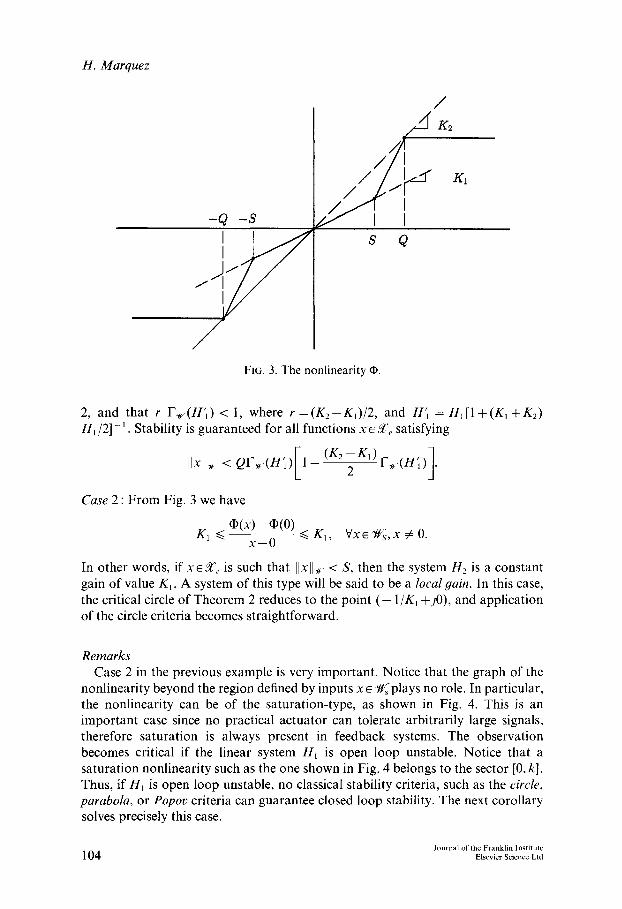
Case 1 : From the graph of the nonlinearity we conclude that

O(x) --O(0) KI ~< ~<K2, Vxsuchthatl lxl] , < Q , x ¢ O .

( x - 0 )

Thus H2 is locally in the sector [KI,/£2] about Xo - 0. Moreover, according to case (a) of the circle criteria, the system is locally stable about xo = 0 provided the Nyquist plot of the linear system is bounded away from the critical circle centred on the real line and passing through the points ( - l/K1 +jO) and ( - l/k: +jO), and encircles it v times in the counterclockwise direction, with v defined as in Theorem

Vol. 332B, No. 1. pp. 91 106. 1995 Printed in Great Britain. All rights reserved 1 0 3

H. Marquez

-0, - S

/

,4

K~

s Q

FIG. 3. The nonlinearity qb.

2, and that r F ~ ( H ' ~ ) < 1, where r=(Kz-KI)/2, and H'l = HI[I+(KI+K2) Hj/2] - i. Stability is guaranteed for all functions x e Y'e satisfying

Ilxll~ < QFu (H'I) [1 (K2-K1)Fu(H'I)]

Case 2 : From Fig. 3 we have

• (x) - . (o) K1 ~ ~< K1, Vx 6 ~/~s, x ¢ 0.

x - 0

In other words, if xeY'e is such that ]lxU, < S, then the system H 2 is a constant gain of value KI. A system of this type will be said to be a local 9ain. In this case, the critical circle of Theorem 2 reduces to the point ( - 1/Ki +jO), and application of the circle criteria becomes straightforward.

Remarks Case 2 in the previous example is very important. Notice that the graph of the

nonlinearity beyond the region defined by inputs x E ~ , plays no role. In particular, the nonlinearity can be of the saturation-type, as shown in Fig. 4. This is an important case since no practical actuator can tolerate arbitrarily large signals, therefore saturation is always present in feedback systems. The observation becomes critical if the linear system H1 is open loop unstable. Notice that a saturation nonlinearity such as the one shown in Fig. 4 belongs to the sector [0, k]. Thus, if H1 is open loop unstable, no classical stability criteria, such as the circle, parabola, or Popov criteria can guarantee closed loop stability. The next corollary solves precisely this case.

Journal of the Franklin Institute 104 Elsevier Science Ltd

Input~Output Stability

-0,

J 7

~ f

O,

./_fK I

FIG. 4. Saturation-type nonlinearity.

Corollary 1 Consider the feedback interconnection of the systems H1 and H 2 : flJf,, --~ 3{',,. Let

HI be defined as in Theorem 2, and let H 2 be a local gain about Xo, i.e. H 2 is such that

H2 [ z - Zo] = K* [ z - Zo], V z such that (z - z,,) e ~/~.

Then, the system is locally input/output stable about xo if the system H] = HI [1 + K ' H 1 ] -1 is ~ - s t ab le for all Q in N, where stability is guaranteed for all input functions satisfying

Q IIx-xoll,, < F,,-(H'I~ (44)

Proof: Define a loop transformation with K = K*. Thus, we obtain

H', = H~ [1 + K ' N i l ~ =~/4', (s) = d(s)/[1 +K*G(s)I

Thus,

H~ = H 2 - K * .

H~ [ z - zo] = (H2 - - K*)[z - Zo]

= H 2 [z - - Zo] - K * [z - - Zo]

= K * [ z - Z o ] - K * [ z - Z o ] = 0 i f l l z -zol l~ < Q.

Thus, if the system H'~ satisfies the Nyquist stability criteria, we have F:r(H]) < m, and F,-(H'I) < m, and then local input/output stability follows trivially from Theorem 1, since F.~(H'2, Zo) = F,.-(H'2, zo) = O,(z-Zo) ~ ~¢U o. The proof is then complete by recognizing that condition (44) guarantees that IIz-zoll~ < Q.

Remarks Corollary 1 gives proper mathematical foundation to a result that has been used

ad hoc by practitioner engineers since the evolution of automatic control systems.

Vol. 332B, No. 1, pp. 91 106, 1995 Printed in Great Britain. All rights reserved 1 0 5

H. Marquez

The result clearly provides the extent of the input/output stability region, a new concept in the control systems literature. Notice that, in general, condition (44) is not a conservative estimate of the class of input functions for which stability is guaranteed. Condition (44) becomes conservative only if the class of input func- tions is somehow restricted to a proper subset of L2 ~ L,~.

V. Conclusions

A local theory of input/output stability of dynamical systems has been outlined. It was shown that by setting the problem in the context of binormed linear spaces it is possible to obtain local versions of the popular small gain theorem and circle criterion. The importance of such a theory relies on the fact that although the input/output representation of a dynamical system is perhaps the most natural one, in the sense that the transformation performed by the system on the space of functions is the true object to be studied in a typical control problem, the math- ematical models used to represent physical systems are usually accurate under somewhat severe restrictions on the space of input functions. In other words, input/output representations of dynamical systems are intrinsically local, and they should not be considered global without proper justification.

References

(1) W. Hahn, "Stability of Motion", Springer-Verlag, New York, 1967. (2) J. P. LaSalle and S. Lefschetz, "Stability by Lyapunov's Direct Method", Academic

Press, New York, 196 I. (3) M. Vidyasagar, "Nonlinear Systems Analysis", Second Edition, Prentice Hall, Engle-

wood Cliffs, NJ, 1993. (4) G. Zames, "Functional analysis applied to nonlinear feedback systems", IEEE Trans.

Circuit Theory, pp. 392-404, September 1963. (5) G. Zames, "On the input/output stability of nonlinear time-varying feedback systems",

Parts I and II, IEEE Trans. Aurora. Control, Vol. AC-11, pp. 228-238 and 465-477, 1966.

(6) 1. W. Sandberg, "An observation concerning the application of the contraction map- ping fixed-point theorem and a result concerning the norm-boundedness of solutions of nonlinear functional equations", Bell Systems Technical Journal, Vol. 44, pp. 1809 1812, 1965.

(7) 1. W. Sandberg, "Some results concerning the theory of physical systems governed by nonlinear functional equations", Bell Syst. Tech. J., Vol. 44, pp. 871-898, May June 1965.

(8) C. A. Desoer and M. Vidyasagar, "Feedback Systems: Input/Output Properties", Academic Press, NY, 1975.

(9) J. C. Willems, "The Analysis of Feedback Systems", MIT Press, Cambridge, MA, 1971.

(10) J. L. Willems, "Stability Theory of Dynamical Systems", Nelson, London, 1970.

Journal of the Franklin Institute 106 Elsevier Science Ltd