a literature review on neuro-cognitive learning and
TRANSCRIPT

A LITERATURE REVIEW ON NEURO-COGNITIVE LEARNING AND CONTROL
By
PATANJALIKUMAR SHASHANKKUMAR JOSHI
Presented to the Faculty of the Graduate School of
The University of Texas at Arlington in Partial Fulfillment
Of the Requirements
For the Degree of
MASTER OF SCIENCE IN ELCTRICAL ENGINEERING
THE UNIVERSITY OF TEXAS AT ARLINGTON
December 2014

ii
Copyright © by Patanjalikumar Shashankkumar Joshi 2014
All Rights Reserved

iii
Acknowledgements
I am very grateful to my supervisor, Dr. Frank Lewis. He has provided excellent guidance
for my research work. His vast knowledge and experience in the area of control systems has
helped me understand various systems in a better way and has inspired to dive deeper research
and some courses like Optimal Control, Distributed Control, Intelligent Control and Nonlinear
Control. I am very happy to get an opportunity to work with him.
Moreover, I would like to thank Dr. Daniel S. Levine and his PhD and Masters students
for facilitating me to understand neuroscience and psychology which were required for my
research work.
Also, I am thankful to PhD students Hamidreza Modares, Bahare Khomartash, Bakur
AlQaudi, Raghavendra Sriram, and Masters student Rubayiat Tousif for providing materials and
guidance whenever asked for. I am also grateful to the support provided by the ONR Grant #
N00014-13-1-0562. Lastly, I thank my family and friends for their encouragement and support.
November 24, 2014

iv
Abstract
A LITERATURE REVIEW ON NEURO-COGNITIVE LEARNING AND CONTROL
Patanjalikumar Shashankkumar Joshi, M.S.
The University of Texas at Arlington, 2014
Supervising Professor: Frank L. Lewis
This thesis is an effort to provide a foundation work linking neuroscience, psychology and
control theory as a part of research going on developing fast satisficing autonomous systems at
the University of Texas at Arlington Research Institute (UTARI). This literature review, the
compilation is aimed to facilitate information and references needed for neurocognition and
control.
There is so much research going on to understand the neural mechanisms of a mammal
brain, especially human brain. Although it is not fully understood, there are proposed and proven
theories that address intelligence, various learning and decision making processes performed by
various parts of the brain. Cerebellum is hypothesized to be responsible for supervised learning,
cerebral cortex for unsupervised learning and basal ganglia for reinforcement learning with help
of dopamine. Probability, the representation of data and emotions do affect the decision process.
A shunting inhibitory neural network which include amygdala, orbitofrontal cortex, ventral
striatum, thalamus and anterior cingulated cortex, is involved when the decision process is
affected by probability and emotions. That is related with gist and verbatim, too. Cognitive abilities
also make difference in decisions. It is proposed that there are multiple learning and control loops
in the brain.
With aim of replicating brain-like intelligence, multiple actor-critics solve Bellman equation
using approximate dynamic programming for optimal control. Multiple model based architectures
for learning and control have been proposed which also find optimal control for systems. These

v
architectures include artificial neural network which utilize shunting inhibition and multiple model
reinforcement learning.
Still, to achieve brain-like intelligence, optimality is not necessary. Satisficing decision has
to only meet only some minimum acceptance; it does not have to be optimal, so it can be faster.
Inclusion of satisficing in multi-player games is beneficial. Also, it is not always possible to make
optimal choices due to various limitations, so with a bounded rationality, choices have to be
made. Finally, the goal is to develop a framework that can learn and control various systems, fast
and efficiently with limited resources and rapidly changing environment.

vi
Table of Contents
Acknowledgements ......................................................................................................................... iii
Abstract............................................................................................................................................ iv
List of Illustrations ............................................................................................................................ ix
Chapter 1 Introduction ......................................................................................................................1
Chapter 2 Work in the 1990’s on Neuro-cognition ...........................................................................3
2.1 Learning and Control in Basal Ganglia and Cerebral Cortex.................................................3
2.1.1 Introduction .................................................................................................................... 3
2.1.2 Supervised Learning in the Cerebellum......................................................................... 4
2.1.3 Reinforcement Learning in the Basal Ganglia ............................................................... 6
2.1.4 Unsupervised Learning in the Cerebral Cortex............................................................ 11
References .................................................................................................................................13
2.2 Brain like Intelligence and Approximate Dynamic Programming.........................................14
2.2.1. Introduction ................................................................................................................. 14
2.2.2 from Optimality to ADP ................................................................................................ 14
2.2.3 First Generation ADP Model ........................................................................................ 15
2.2.4 Second Generation ADP Model................................................................................... 17
2.2.5 Approximate Dynamic Programming ........................................................................... 18
References .................................................................................................................................21
2.3 Outline of Biological Functions of Various Regions in the Brain..........................................22
2.3.1 Introduction .................................................................................................................. 22
2.3.2 Amygdala ..................................................................................................................... 23
2.3.3 Orbito-Frontal Cortex ................................................................................................... 24
2.3.4 Basal Ganglia............................................................................................................... 25
2.3.5 Dorsolateral Prefrontal Cortex ..................................................................................... 26
2.3.6 Anterior Cingulate Cortex............................................................................................. 27
2.3.7 Hippocampus ............................................................................................................... 28

vii
2.3.8 Thalamus ..................................................................................................................... 29
References .................................................................................................................................30
Chapter 3 Neuro-cognitive Psychology ..........................................................................................31
3.1 D. S. Levine’s Work in Neuro-cognitive Psychology............................................................31
3.1.1 Introduction .................................................................................................................. 31
3.1.2 Emotion and Decision Making ..................................................................................... 32
3.1.3 Modeling the Rules of Behavior ................................................................................... 33
3.1.4 The Brain Model........................................................................................................... 35
References .................................................................................................................................42
3.2 Third Generation Brain like Intelligence and Approximate Dynamic
Programming..............................................................................................................................43
3.2.1 Stochastic Encoder/Decoder Predictor........................................................................ 45
References .................................................................................................................................49
3.3 Cognitive Development with a Psychological Perspective ..................................................50
3.3.1 Introduction .................................................................................................................. 50
3.3.2 Decision Making with Rules ......................................................................................... 50
3.3.3 Piaget’s Theory of Cognitive Development.................................................................. 51
3.3.4. Cognition and Decision under Risk............................................................................. 53
References .................................................................................................................................55
Chapter 4 New Neuro-inspired Architectures for Learning and Control.........................................56
4.1 Neuro-inspired Networks for Learning .................................................................................56
4.1.1 Introduction .................................................................................................................. 56
4.1.2 Shunting Inhibitory Artificial Neural Networks.............................................................. 56
4.1.3 Neuro-Inspired Robot Cognitive Control with Reinforcement Learning....................... 61
References .................................................................................................................................65
4.2 Multiple Model Based Learning and Control ........................................................................66
4.2.1 Introduction .................................................................................................................. 66

viii
4.2.2 Multi-Model Adaptive Control....................................................................................... 66
4.2.3 Multiple Model-Based Reinforcement Learning........................................................... 68
4.2.4 Extended Modular Selection and Identification for Control.......................................... 71
References .................................................................................................................................76
Chapter 5 Satisficing ......................................................................................................................77
5.1 Satisficing and Control .........................................................................................................77
5.1.1 What is Satisficing?...................................................................................................... 77
5.1.2 Satisficing Decisions .................................................................................................... 78
5.1.3 Constructive Nonlinear Control using Satisficing......................................................... 80
References .................................................................................................................................84
5.2 Satisficing Games ................................................................................................................85
5.2.1 Satisficing in Game Theory.......................................................................................... 85
References .................................................................................................................................89
Chapter 6 Bounded Rationality.......................................................................................................90
6.1 What is Bounded Rationality? ..............................................................................................90
6.1.1 Introduction .................................................................................................................. 90
6.1.2 Bounded Rationality and Behavioral Psychology: ....................................................... 91
References .................................................................................................................................95
6.2 Metacognition.......................................................................................................................96
6.2.1 Introduction .................................................................................................................. 96
6.2.2 Components of Metacognition ..................................................................................... 96
References .................................................................................................................................99
Bibliography..................................................................................................................................100
Biographical Information...............................................................................................................105

ix
List of Illustrations
Figure 1 Interconnection of the cerebellum, the basal ganglia and the cerebral cortex [2] ............ 4
Figure 2 Cerebellar circuit for supervised learning. •-inhibitory connection, CN-Deep cerebellar
nuclei, IO-Inferior olive, Empty circle-excitatory connection [1]....................................................... 4
Figure 3 Neural circuit of the basal ganglia. SNc-Substantia nigra pars compacta, SNr-Substantia
nigra pars reticula, GPi-Internal segment of globus pallidus, GPe-External segment of globus
pallidus, STN-subthalamic nucleus, O-Excitatory connection, •-Inhibitory...................................... 6
Figure 4 The monkey-reward experiment [4] .................................................................................. 8
Figure 5 Response of dopamine neuron to touch of food reward [7] .............................................. 9
Figure 6 Error of reward prediction detected by the dopamine neurons [7] .................................... 9
Figure 7 Reward expectation-related activity in primate putamen neuron [7] ............................... 10
Figure 8 Unsupervised learning neural circuit of cerebral cortex. P-Pyramidal neurons, S-Spiny
stellate neurons, I-Inhibitory interneurons, o-Excitatory connection, •-Inhibitory connection [1] ... 11
Figure 9 Animal Behavior Choice [2] ............................................................................................. 14
Figure 10 Origins of ANN [2] ......................................................................................................... 15
Figure 11 First possible emergent intelligence [2]......................................................................... 16
Figure 12 Second generation brain model [2] ............................................................................... 17
Figure 13 Adapting critic using HDP [3] ........................................................................................ 19
Figure 14 Adapting critic using DHP [3] ........................................................................................ 20
Figure 15 Human brain.................................................................................................................. 22
Figure 16 Location of amygdala: top view (left image), side view (Right image) .......................... 23
Figure 17 OFC: (a) Side view (b) Top view ................................................................................... 24
Figure 18 Location of basal ganglia in the brain............................................................................ 25
Figure 19 Location of DLPFC ........................................................................................................ 26
Figure 20 Location of ACC ............................................................................................................ 27
Figure 21 Location of Hippocampus.............................................................................................. 28
Figure 22 Location of Thalamus.................................................................................................... 29
x
Figure 23 Typical weighing curve [4] ............................................................................................. 33
Figure 24 Fight-or-flight path. CRF is a biochemical precursor to a stress hormone [6]............... 34
Figure 25 Dissociation pathway. Filled circles denote inhibition. PVN: paraventricular nucleus of
hypothalamus [6]. .......................................................................................................................... 34
Figure 26 Tend-and-befriend pathway. ACh: acetylcholine, DA: Dopamine. Semicircles denote
modifiable synapses [6]. ................................................................................................................ 35
Figure 27 Schematic Gated Dipole. ‘->’ denote excitation, • denote inhibition and partially filled
square denote depletion [1]. .......................................................................................................... 36
Figure 28 Daniel Levine’s network. -> denote excitation, • denote inhibition and partially filled
square denote depletion [4]. .......................................................................................................... 38
Figure 29 Neural Network Model of Brain [1] ................................................................................ 41
Figure 30 Third generation brain model of creativity [1] ................................................................ 43
Figure 31 The SEDP [2] ................................................................................................................ 46
Figure 32 Summary of Human Nervous System........................................................................... 48
Figure 33 Specific rules used by participants as a function of age group [2] ................................ 51
Figure 34 Steady state model of a shunting neuron [4]................................................................. 57
Figure 35 Feedforward SIANN [4] ................................................................................................. 58
Figure 36 Decision regions of SIANN. a1=a2=1, b1=b2=5, w1=-2, w2=2, c12=c21=1, c11=c22=5
[4]. .................................................................................................................................................. 59
Figure 37 Estimated function using SIANN and MLP [4]............................................................... 60
Figure 38 Classification using SIANN and MLP [4] ....................................................................... 61
Figure 39 The neural model [1] ..................................................................................................... 63
Figure 40 A multi-model architecture [5] ....................................................................................... 67
Figure 41 The MMRL architecture [2]............................................................................................ 69
Figure 42 The eMOSAIC model [6] ............................................................................................... 73
Figure 43 Selectability and rejectability functions and satisficing set for particular x and single
input u [3] ....................................................................................................................................... 81

xi
Figure 44 Cognitive system architecture [2] .................................................................................. 92
Figure 45 Different accessibility dimension example [2] ............................................................... 93

1
Chapter 1
Introduction
The term "intelligent control" has been used in a variety of ways. To us, "intelligent
control" should involve both intelligence and control theory. It should be based on a serious
attempt to understand and replicate the phenomena that we have always called "intelligence"-i.e.,
the generalized, flexible, and adaptive kind of capability that we see in the human brain. There
are five chapters which provide information related to the above mentioned areas. Each chapter
is further divided into sections which group similar aspects.
Chapter 2 discusses some of the earliest work done to understand and model learning
and decision process done in the brain. It has three sections. The first section describes the work
done by Kenji Doya, W. Schultz and others that focus on process in basal ganglia and cerebral
cortex. The second section talks about work done by Paul Werbos who suggested various ADP
models of the brain. The third section discusses about various parts of the brain involved in the
decision process.
Chapter 3 also talks about cognitive development from psychological perspective. The
first section puts together the effort done by Daniel Levine to model the decision process in the
brain which mainly involves orbitofrontal cortex, amygdala and relates emotion, risk and
probability to decision. The second section talks about Paul Werbos newer work in ADP. The
third section illustrates cognitive abilities and decision making from psychological studies which
involves Piaget’s theory of cognitive development.
Chapter 4 takes a look at the new, neuro-cognitively developed learning and control
mechanisms. The first section discusses learning structures which include reinforcement learning,
fuzzy logic and shunting inhibitory artificial neural networks. Inspired and understood through all
the neuro-physiological studies, multiple actor-critic architecture is used for model prediction and
control. This involves multiple model based reinforcement learning, parallel neural networks,
multiple model based adaptive control and the eMOSAIC model.

2
Chapter 5 is about satisficing which is different from optimality. With the time and
resource constraints, optimality is not always needed. Also this can result in faster decisions. The
first section discusses about satisficing control theory. The second section is application of
satisficing in game theory which results in satisficing games. Satisficing is like having something
good or better which is not the best; it sounds more like just getting satisfied.
Chapter 6 talks about bounded rationality. The first section explains the concept of
bounded rationality. It is related to psychology, economics and management. Its impact also been
studied in peer-to-peer networks. The second section illustrates metacognition which is a state of
‘knowing of knowing’. It is related with bounded rationality and satisficing.
This work is aimed at providing links between neuroscience, psychology and control
systems. Detailed study of mechanism of computations and decisions in human brain has been
presented. It is further strengthened with findings from a psychological perspective. Concepts of
satisficing and bounded rationality are included. Architectures for learning and control which are
inspired through, and use all these findings are presented so that an integrated compilation has
been prepared on basis of which faster, more efficient decisions and control structures can be
designed for various autonomous systems.

3
Chapter 2
Work in the 1990’s on Neuro-cognition
2.1 Learning and Control in Basal Ganglia and Cerebral Cortex
This section discusses roles played by the cerebral cortex and basal ganglia in various
learning processes and control. It involves work done by Kenji Doya [1, 2, and 3] and Wolfram
Schultz [4-8]. Both, neurophysiology and mathematics of the brain processes are illustrated. To
further explain the reward prediction during reinforcement learning, a study and its findings have
been also included.
Equation Chapter 2 Section 1
2.1.1 Introduction
It was originally believed that the cerebellum and the basal ganglia were dedicated to
only motor control. But more and more evidence is being found suggesting their involvement in
non-motor tasks [1, 2]. By studying anatomical features of their structures Doya suggests that the
cerebellum, the basal ganglia and the cerebral cortex are each specialized for a particular kind of
computation. They are reciprocally connected with each other (Fig. 1) and simultaneously active
[2]. A theory is proposed that the cerebellum implements ‘supervised learning’, the basal ganglia
‘reinforcement learning’ and the cerebral cortex implements ‘unsupervised learning’ [1].

4
Figure 1 Interconnection of the cerebellum, the basal ganglia and the cerebral cortex [2]
2.1.2 Supervised Learning in the Cerebellum
Figure 2 Cerebellar circuit for supervised learning. •-inhibitory connection, CN-Deep cerebellar
nuclei, IO-Inferior olive, Empty circle-excitatory connection [1]

5
The cerebellum circuit for the supervised learning is shown in the figure 2. It has a nearly
feed-forward structure with massive synaptic convergence of granule cell (GC) axons (parallel
fibers) onto purkinje cells (PC). The purkinje cells receive inputs from both parallel fibers and the
climbing fiber. The output is provided by the neurons located in the deep cerebellar nuclei. An
input-output mapping is computed through the supervised learning [1].
( )Fy x (2.1.1)
where the output 1( ,..., y )myy ’ and the input 1( ,..., )nx xx ’.
The movement related signals are encoded by the purkinje cells’ simple spike responses
to parallel fiber input and the errors in movement are encoded by the climbing fiber. The mapping
is found from the desired output ˆ ˆ( (1), (2),...)y y in order to minimize the expected output error
such as [1],
2ˆE x y y (2.1.2)
In case of unknown distribution of the input, it can be approximated by minimizing the sum of
squared errors at sample data points
2 2ˆ ˆ( ) ( ) ( ) ( (t); )t t
E t t t F y y y x w (2.1.3)
under a certain constraint on the mapping F. The outputs of the granule cells are linearly
combined by a purkinje cells as [1]
1
( ) ( ),n
i ij jj
y t w x t
(2.1.4)
where wij is a synaptic connection weight and it can be updated/learned by the gradient descent
of the sample error [1]
ˆ ( ) ( ) ( ),ij i i jij
Ew y t y t x t
w
(2.1.5)
That is, the parameter updates based on the correlation between the output error and the
presynaptic input [1].

6
2.1.3 Reinforcement Learning in the Basal Ganglia
Figure 3 Neural circuit of the basal ganglia. SNc-Substantia nigra pars compacta, SNr-Substantia
nigra pars reticula, GPi-Internal segment of globus pallidus, GPe-External segment of globus
pallidus, STN-subthalamic nucleus, O-Excitatory connection, •-Inhibitory
The circuit of the basal ganglia implementing reinforcement learning is shown figure 3.
The main input from the cerebral cortex goes to the striatum which consist of a part called
striosome and a part called matrix. A learning agent takes an action u(t) ∈ Rm in response to the
state x(t) ∈ Rn of the environment [1].
( 1) ( ( ), ( ))t F t t x x u (2.1.6)When an unexpected reward or a sensory cue signaling the delivery of a reward in near future is
related with phasic increase in firing of dopamine neurons in SNc. The reward [1]
( 1) ( ( ), ( ))r t R t t x u (2.1.7)The matrix compartment selects the action which maximizes the cumulative sum of rewards [1]
( ) ( ( ))t G tu x (2.1.8)The striosome plays the role of value prediction mechanism for the maximization mentioned
above [1]
2( ) ( 1) ( 2) ( 3) ...V E r t r t r t x (2.1.9)
where a discount factor 0 1 .
The value function can be learned by minimizing the ‘temporal difference’ (TD) error of
the reward prediction which is encoded by the dopamine neuron activity [1]
7
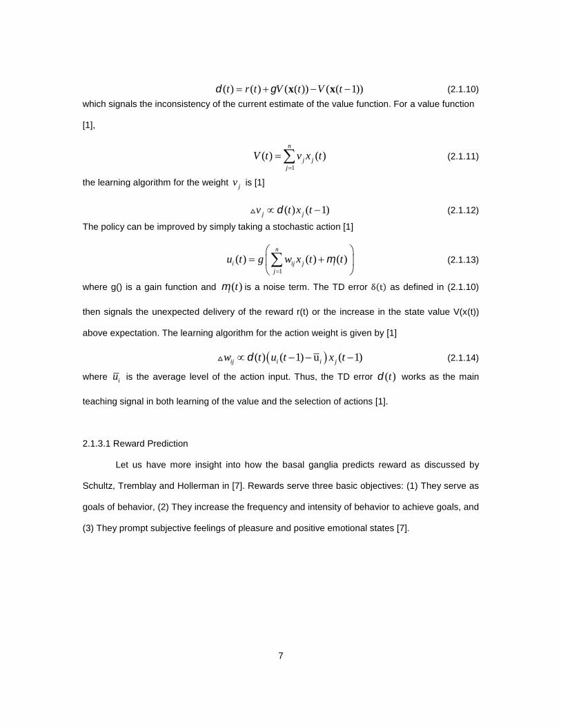
( ) ( ) ( ( )) ( ( 1))t r t V t V t x x (2.1.10)which signals the inconsistency of the current estimate of the value function. For a value function
[1],
1
( ) ( )n
j jj
V t v x t
(2.1.11)
the learning algorithm for the weight jv is [1]
( ) ( 1)j jv t x t (2.1.12)
The policy can be improved by simply taking a stochastic action [1]
1
( ) ( ) ( )n
i ij j ij
u t g w x t t
(2.1.13)
where g() is a gain function and ( )i t is a noise term. The TD error δ(t) as defined in (2.1.10)
then signals the unexpected delivery of the reward r(t) or the increase in the state value V(x(t))
above expectation. The learning algorithm for the action weight is given by [1]
( ) ( 1) u ( 1)ij i i jw t u t x t (2.1.14)
where iu is the average level of the action input. Thus, the TD error ( )t works as the main
teaching signal in both learning of the value and the selection of actions [1].
2.1.3.1 Reward Prediction
Let us have more insight into how the basal ganglia predicts reward as discussed by
Schultz, Tremblay and Hollerman in [7]. Rewards serve three basic objectives: (1) They serve as
goals of behavior, (2) They increase the frequency and intensity of behavior to achieve goals, and
(3) They prompt subjective feelings of pleasure and positive emotional states [7].
8
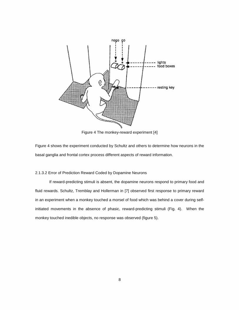
Figure 4 The monkey-reward experiment [4]
Figure 4 shows the experiment conducted by Schultz and others to determine how neurons in the
basal ganglia and frontal cortex process different aspects of reward information.
2.1.3.2 Error of Prediction Reward Coded by Dopamine Neurons
If reward-predicting stimuli is absent, the dopamine neurons respond to primary food and
fluid rewards. Schultz, Tremblay and Hollerman in [7] observed first response to primary reward
in an experiment when a monkey touched a morsel of food which was behind a cover during self-
initiated movements in the absence of phasic, reward-predicting stimuli (Fig. 4). When the
monkey touched inedible objects, no response was observed (figure 5).

9
Figure 5 Response of dopamine neuron to touch of food reward [7]
Figure 6 Error of reward prediction detected by the dopamine neurons [7]
It can be seen that the dopamine neurons are also activated when reward is presented
without any stimulus during learning (Fig. 6, top). After learning the task, the dopamine response
occurs after the reward-predicting conditioned stimulus and depletes after the reward (figure 6,

10
middle). If a fully predicted reward does not occur when it should have occurred, then at that time
the activity of the dopamine neurons is depressed (figure 6, bottom). This suggests that
dopamine neurons encode the error in prediction of reward. Learning slows down as the
prediction error decreases and the outcome is predicted more accurately. It is suggested that the
dopamine response is a scalar reinforcement signal provided simultaneously to all neurons in the
striatum, although dopamine neurons cannot discriminate between different rewards [7].
2.1.3.3 Learning Changes in Reward Expectation by Striatal Neurons
Schultz and the others in [7] found that the neurons in the striatum have access to central
stored representations of experiences of previous individual task events which also includes the
rewards. As show in figure 7, the reward expectation-related activations did not occur with
unrewarded movements; but occurred only during external reinforcements.
Figure 7 Reward expectation-related activity in primate putamen neuron [7]
Some of these activations were able to distinguish between different types of reward. It
indicates that the striatal neurons can access previous and current expectation-related activity
information and update/adapt them according to novel situation. Thus, they can validate and
provide accurate information about rewards in advance. This is very much different from the
activity of dopamine neurons which encode the temporal difference error between prediction and
actual occurrence of the reward [7].

11
2.1.4 Unsupervised Learning in the Cerebral Cortex
Figure 8 Unsupervised learning neural circuit of cerebral cortex. P-Pyramidal neurons, S-
Spiny stellate neurons, I-Inhibitory interneurons, o-Excitatory connection, •-Inhibitory connection
[1]
It can be seen in figure 11 that the cerebral cortex has a layered organization and
massive recurrent connections. The cerebral cortex has different functional areas representing
sensory, motor or contextual information in different modalities and frames of reference. The
statistical properties of the inputs are characterized by a mapping constructed from a set of input
data (x(1), x(2), …,) ∈ Rn to the output (y(1), y(2), …,) ∈ Rm. One way to maximize the mutual
information between the input and the output as defined in [1],
( ; ) ( ) ( | )H H H x y x x y (2.1.15)
where H denotes the entropy ( ) log ( )H E p x x . It enumerates the decrease in uncertainty
about input x by knowing output y. An objective function can be used to derive an unsupervised
algorithm [1]
2
1
( ) ( ) ( )m
ii
E t W t y t
x y (2.1.16)
where W is the input-output weight matrix, the first term represents the input reconstruction error
and the second term embodies a sparseness constraint. This yields maximization of the mutual
information and reassurance of the majority of outputs to be close to zero [1].
The information coding of the neurons in the cerebral cortex can be determined by the
relaxation dynamics [1]

12
sign( )E
W WW
y x y yy
(2.1.17)
The synapses’ weights are updated by a Hebbian rule given by the gradient descent [1]
( )E
W W WW
y x y yx yy (2.1.18)

13
References
1. Kenji Doya, “What are the computations of the cerebellum, the basal ganglia and the
cerebral cortex?” Neural Networks 12, 1999, pp. 961-974.
2. Kenji Doya, Hidenori Kimura, Mitsuo Kawato, “Neural Mechanisms of Learning and
Control,” IEEE Control System Magazine, Vol. 21, 2001, pp. 42-54.
3. Kenji Doya, Hidenori Kimura, Aiko Miyamura, “Motor control: neural models and system
theory”, International Journal of Applied Mathematics and Computer Science, Vol. 11, 2001, pp.
101-128.
4. Wolfram Schultz, Ranuifo Romo, “Role of primate basal ganglia and frontal cortex in the
internal generation of movements-I. Preparatory activity in the anterior striatum”, Experimental
Brain Research 91, 1992, pp. 363-384.
5. Ranuifo Romo, Eugenio Scarnati, Wolfram Schultz, “Role of primate basal ganglia and
frontal cortex in the internal generation of movements-II. Movement related activity in the anterior
striatum”, Experimental Brain Research 91, 1992, pp. 385-395.
6. Ranuifo Romo, Wolfram Schultz, “Role of primate basal ganglia and frontal cortex in the
internal generation of movements-III. Neuronal activity in the anterior striatum”, Experimental
Brain Research 91, 1992, pp. 396-407.
7. Wolfram Schultz, Leon Tremblay, Jeffrey R. Hollerman, “Reward prediction in primate
basal ganglia and frontal cortex”, Neuropharmacology 37, 1998, pp. 421-429.
8. Wolfram Schultz, Leon Tremblay, Jeffrey R. Hollerman, “Reward processing in primate
orbitofrontal cortex and basal ganglia”, Cerebral Cortex, 2007, pp. 272-283.

14
2.2 Brain like Intelligence and Approximate Dynamic Programming
Equation Chapter 2 Section 2
In this section, I have discussed some of the initial efforts done by Paul Werbos [1-4] to
design and develop brain-like intelligence. He tried to combine neuro-physiology and control
system theory. In the process, he developed a concept of Approximate Dynamic Programming
(ADP). Here, the first and second generation models of ADP are discussed. The third generation
ADP model is discussed in section 3.2.
2.2.1. Introduction
Werbos’ work explains the basic mathematical principles and their relation to the most
important features of a mammal brain‒how intelligence works so that a control system can be
designed that can learn to perform the complex range of tasks. As even a mouse has a structure
like six-layer neocortex and it shows general purpose learning abilities, understanding the mouse
brain is an important step toward understanding the human mind [2]. From this, approximate
dynamic programming emerges which combines control theory and neural networks.
2.2.2 from Optimality to ADP
People have tried to understand the human brain using the idea of optimization.
Animal behavior is finally about choices as shown in the figure 9.
Figure 9 Animal Behavior Choice [2]
The rules of the action selection can be fixed for a simple animal; while they can be
selected based on the computed outcomes for the taken actions for an advance animal. Werbos
[2] defines functionality as an ability of the brain about making choices which yield better results;

15
while Intelligence as an ability of the brain about learning how to make better choices. But all this
has to be put into mathematics to have a way to find the better result [2].
Now one may wonder that if brains are so optimal, then also humans do so many stupid
things! This can be explained by Von Neumann’s Cardinal Utility function which is the foundation
of decision theory and dynamic programming among others. The brains are designed to learn
approximate optimal policy with bounded computational resources. They never learn to play a
perfect game of chess! Over the course of time, various ADP models of brain intelligence have
been developed.
2.2.3 First Generation ADP Model
Figure 10 Origins of ANN [2]
As shown in figure 10, both back-propagation and the first ADP design originated in
Werbos’ work. It was proposed after many tried to develop brain like intelligence that the decision
system which can learn to approximate the Bellman equation could be built (1971-72). With
noise, an optimal strategy or policy of action for a general nonlinear decision problem can be
computed efficiently [2].
( )
( ( )) max ( ( ), ( )) ( ( 1)) / 1t
J t U t t J t r u
x x u x (2.2.1)
16
where ( )tx is the state of the environment at time t, ( )tu is the choice of actions, U is the
cardinal utility function, r is the interest or discount rate, the angle brackets denote expectation
value and J is the function that must be solved in order to derive an optimal strategy of action.
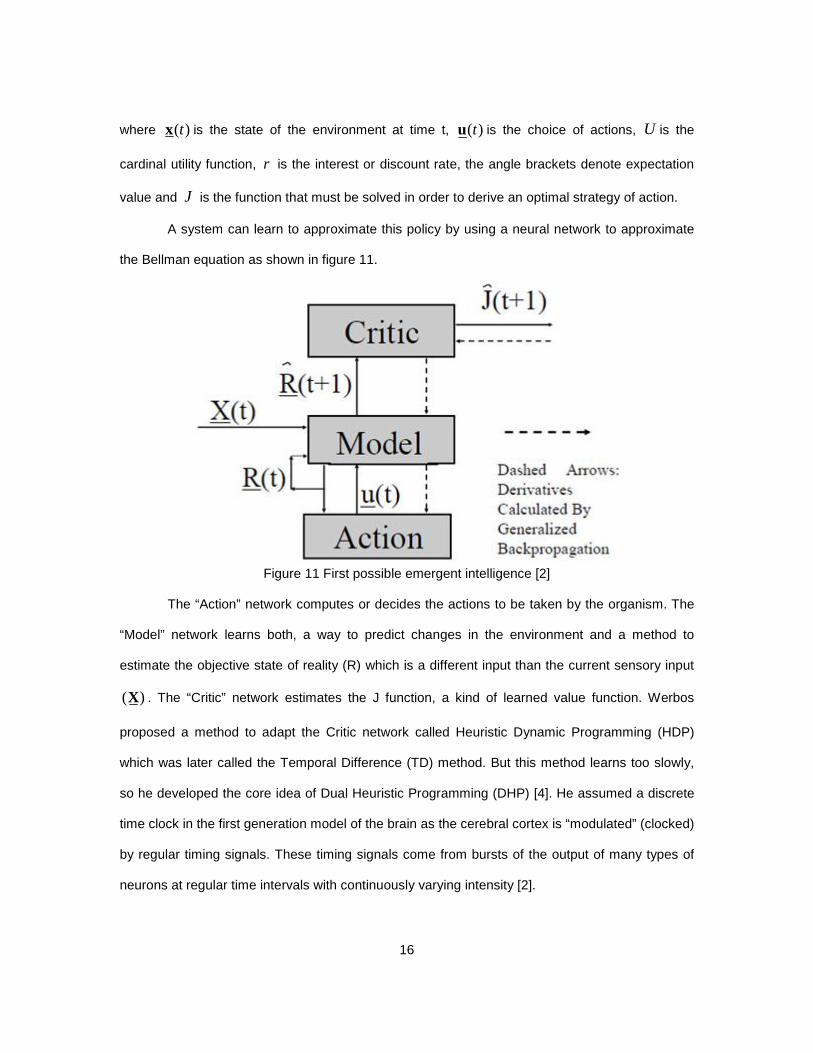
A system can learn to approximate this policy by using a neural network to approximate
the Bellman equation as shown in figure 11.
Figure 11 First possible emergent intelligence [2]
The “Action” network computes or decides the actions to be taken by the organism. The
“Model” network learns both, a way to predict changes in the environment and a method to
estimate the objective state of reality (R) which is a different input than the current sensory input
( )X . The “Critic” network estimates the J function, a kind of learned value function. Werbos
proposed a method to adapt the Critic network called Heuristic Dynamic Programming (HDP)
which was later called the Temporal Difference (TD) method. But this method learns too slowly,
so he developed the core idea of Dual Heuristic Programming (DHP) [4]. He assumed a discrete
time clock in the first generation model of the brain as the cerebral cortex is “modulated” (clocked)
by regular timing signals. These timing signals come from bursts of the output of many types of
neurons at regular time intervals with continuously varying intensity [2].

17
2.2.4 Second Generation ADP Model
Werbos proposed a second generation ADP model in 1987 as shown in figure 16.
Figure 12 Second generation brain model [2]
It was motivated both by trying to understand the brain and by an engineering dilemma.
The critic and actor networks required more powerful networks than feed-forward neural
networks. It requires use of recurrent networks which give out the result after many cycles of
inner loop computations. This low sampling rate is observed for the cerebral cortex responding to
inputs from the thalamus, while muscle control is done at a much higher rate. This is similar to a
master-slave system. Werbos suggested an error critic along with a fast model-free slave neural
network model. The purkinje cells of the cerebellum are modeled as memory neurons in the
action network which estimated the vector R. The training is done by a distributed DHP-like critic
system. A strong, stable continuous time model free ADP design like the maser-slave
arrangement has been formulated [2].
18
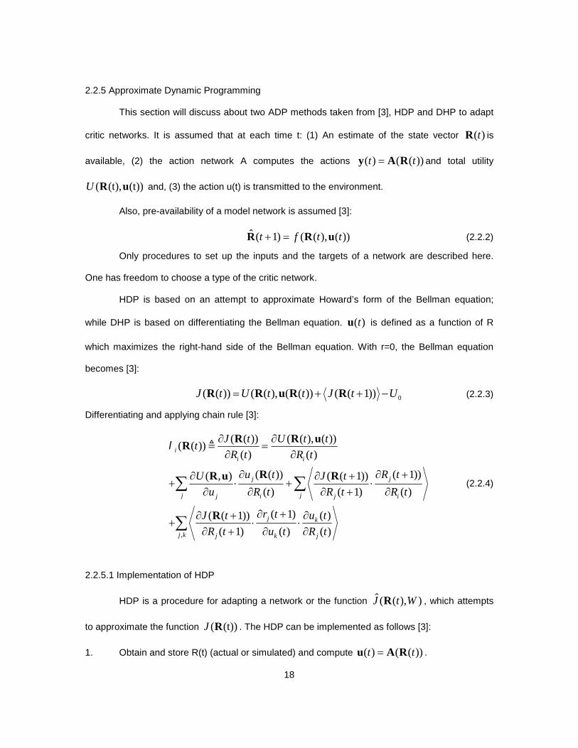
2.2.5 Approximate Dynamic Programming
This section will discuss about two ADP methods taken from [3], HDP and DHP to adapt
critic networks. It is assumed that at each time t: (1) An estimate of the state vector ( )tR is
available, (2) the action network A computes the actions ( ) ( ( ))t ty A R and total utility
( (t), (t))U R u and, (3) the action u(t) is transmitted to the environment.
Also, pre-availability of a model network is assumed [3]:
ˆ ( 1) ( ( ), ( ))t f t t R R u (2.2.2)
Only procedures to set up the inputs and the targets of a network are described here.
One has freedom to choose a type of the critic network.
HDP is based on an attempt to approximate Howard’s form of the Bellman equation;
while DHP is based on differentiating the Bellman equation. ( )tu is defined as a function of R
which maximizes the right-hand side of the Bellman equation. With r=0, the Bellman equation
becomes [3]:
0( ( )) ( ( ), ( ( )) ( ( 1))J t U t t J t U R R u R R (2.2.3)
Differentiating and applying chain rule [3]:
,
( ( )) ( ( ), ( ))( ( ))
( ) ( )
( ( )) ( 1))( , ) ( ( 1))
( ) ( 1) ( )
( 1) ( )( ( 1))
( 1) ( ) ( )
ii i
j j
j jj i j i
j k
j k j k j
J t U t tt
R t R t
u t R tU J t
u R t R t R t
r t u tJ t
R t u t R t
R R uR
RR u R
R
(2.2.4)
2.2.5.1 Implementation of HDP
HDP is a procedure for adapting a network or the function ˆ( ( ), )J t WR , which attempts
to approximate the function ( (t))J R . The HDP can be implemented as follows [3]:
1. Obtain and store R(t) (actual or simulated) and compute ( ) ( ( ))t tu A R .

19
2. Obtain R(t+1) by waiting until t+1 or by predicting ( 1) ( ( ), ( ))t f t t R R u .
3. Calculate:
* ˆ( ) ( ( ), (t)) ( ( 1), ) / (1 )J t U t J t W r R u R (2.2.5)
5. Update W in ˆ( ( ), )J t WR based on inputs R(t) and target *( )J t by using any real time
supervised learning method.
Figure 13 Adapting critic using HDP [3]
2.2.5.1 Implementation of DHP
DHP is a procedure for adapting a critic network or function ˆ( ( ))t R which attempts to
approximate the function ( )i t defined in equation (2.2.4). Any supervised learning method can
be used to adapt the critic in DHP. As use of back-propagation is not required in the supervised
learning, convergence speed is not an issue in DHP. Still, the calculation of target vector * does
use dual subroutines to back-propagate derivatives through the model network and the action
network as shown in figure 14. DHP can be implemented by as follows [3]:
1. Obtain ( ), (t)tR u and R(t+1) as was done with HDP.
2. Calculate:
ˆ ˆ( 1) ( ( 1), W)t t R (2.2.6)

20
ˆ_ (t) _U ( ( ), ( ) _ ( ( ), ( ), ( 1))F t t F f t t t u uF u R u R u (2.2.7)
* ˆ( ) _ ( ( ), ( ), ( 1)) _ ( ( ), ( )) _ ( ( ), _ (t))t F f t t t F U t t F A t R R RR u R u R F u (2.2.8)
3. Update W in ˆ( ( ), )t W R based on the inputs R(t) and target vector *( ).t
Figure 14 Adapting critic using DHP [3]

21
References
1. Paul Werbos, “What is Mind? What is Consciousness? How Can We Build and
Understand Intelligent Systems?”, Werbos’ website.
2. Paul J. Werbos, “Using ADP to Understand and Replicate Brain Intelligence: the Next
Level Design”, IEEE International Symposium on Approximate Dynamic Programming
and Reinforcement Learning, 2007, pp. 209-216.
3. Paul J. Werbos, “Handbook of Intelligent Control: Neural, Fuzzy and Adaptive
Approaches”, VAN NOSTRAND REINHOLD, 1992, pp. 493-525.
4. Paul J. Werbos, “Neural networks and the human mind: New mathematics fits
humanistic insight”, IEEE International Conference on Systems, Man, and Cybernetics,
vol. 1, 1992, pp. 78-83.

22
2.3 Outline of Biological Functions of Various Regions in the Brain
This section talks about various parts of a human brain involved in decision process,
especially the limbic system. Also, their function and location in the brain are discussed.
2.3.1 Introduction
Figure 15 shows the brain regions and their locations together. The following sections
illustrate process involvement, inter-connections and locations of amygdala, orbito-frontal cortex,
basal ganglia, dorsolateral prefrontal cortex, anterior cingulate cortex, hippocampus and
thalamus.
Figure 15 Human brain

23
2.3.2 Amygdala
Figure 16 Location of amygdala: top view (left image), side view (Right image)
Amygdala is an almond-shaped group of nuclei which is located deep and medially within
the temporal lobes of the brain. It is a part of the limbic system. It has connections with
hypothalamus and dorsomedial thalamus. It is found to be primarily involved in memory
processing, decision-making, and emotional reactions. The right and left amygdala perform
different functions. It has been found that the right amygdala induces negative emotions,
especially fear and sadness; while the left amygdala induces either pleasant (happiness) or
unpleasant (fear, anxiety, sadness) emotions and is involved in the brain’s reward computation.
The amygdala is involved in the formation and storage of memories associated with emotions [1].

24
2.3.3 Orbito-Frontal Cortex
Figure 17 OFC: (a) Side view (b) Top view
The orbitofrontal cortex (OFC) is a prefrontal cortex region in the frontal lobes in
the brain. It is located immediately above the eyes. It is a part of the prefrontal cortex that
receives projections from the magnocellular, medial nucleus of the mediodorsal thalamus. It is
involved in the cognitive processing of decision-making. Sensory cortices additionally share
highly complex reciprocal connections with the orbitofrontal cortex. All sensory modalities are
represented in connections with the orbitofrontal cortex, including extensive innervations from
areas associated with olfaction and gustatory somatic responses. It is also connected with
amygdala, hippocampus, striatum and hypothalamus. There is suggestion of a role for the
orbitofrontal cortex in both inhibitory and excitatory regulation of autonomic function. The cortico-
striatal networks seem to be involved in the processing of goal-directed and habitual action,
cortico-limbic connection for a role in action selection, and the integration of information into
behavioral output. It is involved with amygdala in representation of emotion and in decision
making [1].
25
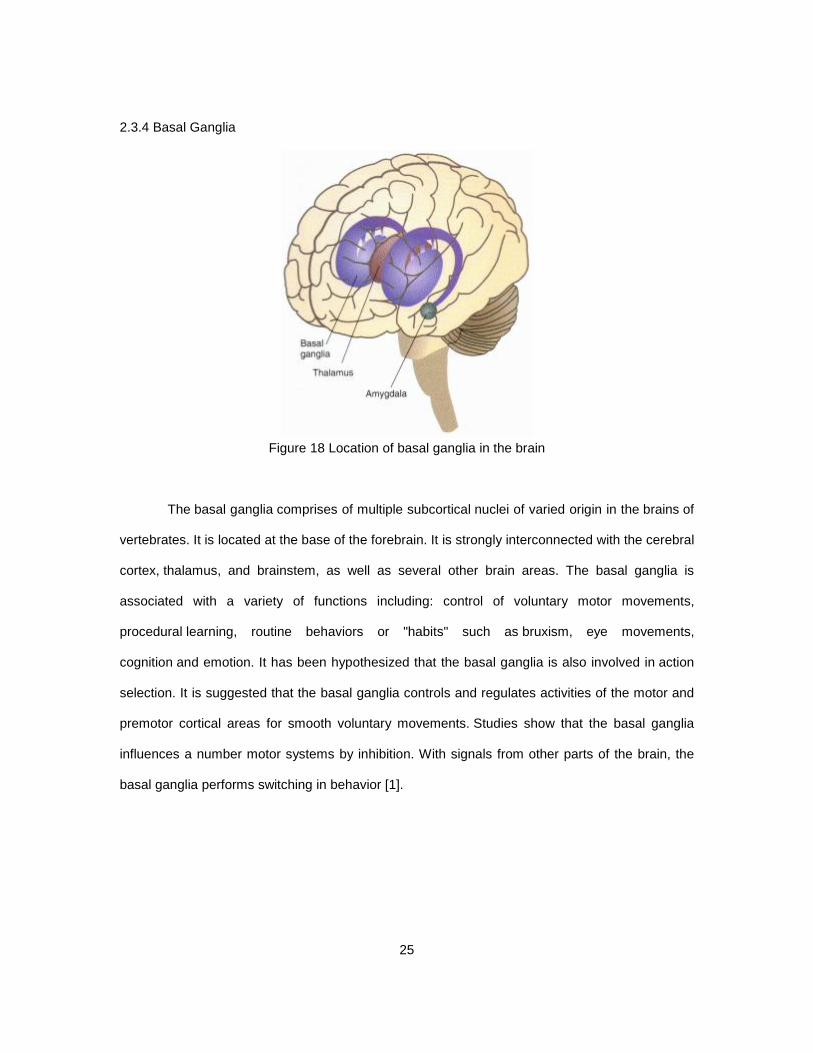
2.3.4 Basal Ganglia
Figure 18 Location of basal ganglia in the brain
The basal ganglia comprises of multiple subcortical nuclei of varied origin in the brains of
vertebrates. It is located at the base of the forebrain. It is strongly interconnected with the cerebral
cortex, thalamus, and brainstem, as well as several other brain areas. The basal ganglia is
associated with a variety of functions including: control of voluntary motor movements,
procedural learning, routine behaviors or "habits" such as bruxism, eye movements,
cognition and emotion. It has been hypothesized that the basal ganglia is also involved in action
selection. It is suggested that the basal ganglia controls and regulates activities of the motor and
premotor cortical areas for smooth voluntary movements. Studies show that the basal ganglia
influences a number motor systems by inhibition. With signals from other parts of the brain, the
basal ganglia performs switching in behavior [1].

26
2.3.5 Dorsolateral Prefrontal Cortex
Figure 19 Location of DLPFC
The dorsolateral prefrontal cortex (DLPFC) is an area in the prefrontal cortex of the brain.
The prolonged maturation of the DLPFC lasts until adulthood. It is basically a functional region
which lays in the middle frontal gyrus of the brain. The DLPFC is connected to orbitofrontal
cortex, thalamus, parts of the basal ganglia, the hippocampus, posterior temporal, parietal, and
occipital areas. Also, the DLPFC provides methods to interact with the stimuli. It plays role in
working memory, cognitive flexibility, planning, inhibition, and abstract reasoning. But, it does
require assistance from other cortical and subcortical areas for complex activities like motor
planning, organization and regulation [1].
27
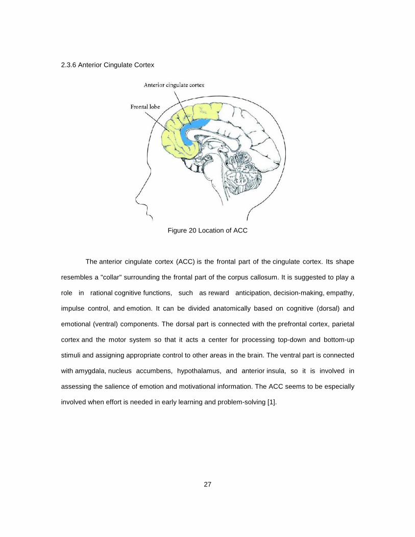
2.3.6 Anterior Cingulate Cortex
Figure 20 Location of ACC
The anterior cingulate cortex (ACC) is the frontal part of the cingulate cortex. Its shape
resembles a "collar" surrounding the frontal part of the corpus callosum. It is suggested to play a
role in rational cognitive functions, such as reward anticipation, decision-making, empathy,
impulse control, and emotion. It can be divided anatomically based on cognitive (dorsal) and
emotional (ventral) components. The dorsal part is connected with the prefrontal cortex, parietal
cortex and the motor system so that it acts a center for processing top-down and bottom-up
stimuli and assigning appropriate control to other areas in the brain. The ventral part is connected
with amygdala, nucleus accumbens, hypothalamus, and anterior insula, so it is involved in
assessing the salience of emotion and motivational information. The ACC seems to be especially
involved when effort is needed in early learning and problem-solving [1].

28
2.3.7 Hippocampus
Figure 21 Location of Hippocampus
Hippocampus belongs to the limbic system. It is located under the cerebral cortex and
divided in each side of the brain. It is connected with the prefrontal cortex, the septum, the
hypothalamic mammillary body, and the anterior nuclear complex in the thalamus. It plays
important roles in the consolidation of information from short-term memory to long-term
memory and spatial navigation. A form of neural plasticity known as long-term potential occurring
in the hippocampus is believed to be one of the reasons of consolidation of the memory. In many
studied it has been found that a damage to the hippocampus affects memory function. Also, a
perception of location in the environment is affected if the hippocampus is damaged [1].

29
2.3.8 Thalamus
Figure 22 Location of Thalamus
Thalamus is a midline symmetrical structure consisting of two halves. It is located
between the cerebral cortex and the midbrain. The thalamus is manifoldly connected to the
hippocampus. Its plays a role in relay of sensory and motor signals to the cerebral cortex, and the
regulation of consciousness, sleep, and alertness. A sensory tract originating in the spinal cord
transmits information to the thalamus about pain, temperature, itch and crude touch. It may be
thought of as a kind of switchboard of information. The thalamus is believed to process the
sensory information also, and it regulates states of sleep, arousal, the level of awareness and
activity [1].

30
References
1. Amygdala, OFC, Basal Ganglia, DLPFC, ACC and Hippocampus from Wikipedia.
2. R. Nieuwenhuys, J. Voogd, C. van Huijzen, “The Human Central Nervous System”, Forth
Edition, Springer (Book), 2008.

31
Chapter 3
Neuro-cognitive Psychology
3.1 D. S. Levine’s Work in Neuro-cognitive Psychology
In this section, Daniel Levine’s work in the area of neuro-cognition is discussed. Effects of
emotions, probability and risk on decision process are investigated. Also, involvement of brain
regions during different types of behaviors are discussed. Then a decision process model of the
brain incorporating gated dipole, adaptive resonance theory and fuzzy trace theory are illustrated.
3.1.1 Introduction
Future autonomous systems require increased speed and dynamical responsiveness of
individual and of groups of coordinated multiple platforms. Due to large data availability, novel
decision and control schemes are required that focus relatively on the data that are relevant for
the current situation and ignore relatively unimportant details. Asymmetric human-robot systems
and demands for fast response impose new requirements for fast and efficient decision,
interaction and control in large distributed teams with autonomous dynamical subsystems.
Streamlined and fast mechanisms that deliver prescribed aspiration levels of satisfactory results
are observed in nature and in neuro-cognitive studies of human brain. Here, rigorous modeling of
mechanisms for fast satisficing, risk, gist and emotional triggers based on new developments in
cognitive neuroscience has been studied. They will be used to develop new structures of
automatic control systems that are capable of fast satisficing, dynamic focusing of awareness and
reduced response times in networked environments.

32
3.1.2 Emotion and Decision Making
3.1.2.1 Short-term Reactions versus Long-term Evaluations
Emotion affects decisions at various times: a guide to information, a selective attentional
spotlight, a motivator of behavior and a common currency of comparing alternatives. While
discussing the relationship of emotion and cognition in the human brain, ‘short-term emotional
reactions’ are needed to be distinguished from ‘long-term emotional evaluations’ [1].
Short-term emotional reactions are related with changes in affective values of rewarding
or punishing stimuli whether it arrives, is removed or changes in intensity; while long-term
emotional evaluations are related with handling the actual affective values of the stimuli rather
than changes in those values. The stimuli either keeps a constant positive or negative value over
time or the value is averaged. Both systems are equally important: The short-term processing
system facilitates effective adaption to sudden salient changes in the environment; while the long-
term emotional processing system it provides effective sensitivity to almost constant attributes in
the environment [1].
3.1.2.2 Probabilistic Choices
One aspect of human decision making is the nonlinear weighting of probabilities. It is
observed that decision makers overweight low nonzero probabilities and underweight low
nonzero probabilities when gambles are explicitly described A low nonzero probability of
obtaining an affect-rich resource (1% probability of obtaining kiss) is more strongly over-weighted
than the same low probability of obtaining an affect-poor resource (1% probability of obtaining
$50) [4]. But, when decisions are made from experience (learning through feedback), the decision
makers typically underweight low probabilities rather than overweighting them! [5].
3.1.2.3 Rational versus Irrational Choices
The work of Reyna and Brainerd suggested ‘fuzzy trace theory’ (FTT) that humans
encode information in two different ways: ‘verbatim’ and ‘gist’ encoding. Verbatim encoding

33
means perception of literal meaning, facts or numerical values; while gist encodes only essential
meaning, intuition. Faster and efficient decision can be achieved when unimportant, minor details
are neglected and the gist of a problem is grasped along with comparison with previously
encountered problems. However, sometimes gist processing using heuristics can lead to errors.is
also a main source of heuristics that can sometimes lead to errors, making irrational choices
instead of rational ones [3]. Methods of gist encoding are unknown and varies within individuals.
Emotions do affect encoding of information. So, a typical weight probability function as shown in
figure 23 was interpreted by Levine (2011) as a nonlinear average of an all-or-none step function
arising from gist encoding and a linear function arising from verbatim coding [2].
Figure 23 Typical weighing curve [4]
3.1.3 Modeling the Rules of Behavior
According to Levine [6], some behavioral patterns are based on evolution and they
prevail in all humans, like the patterns of self-protection and of social bonding behaviors.
Everyone has different criteria for time of engagement in a particular behavior. They are heavily
affected by learning and by culture; not just by genes. So along with Eisler, Levine proposed
cortical-subcortical neural pathways for three separate behavioral patterns: (1) fight-or-flight
(figure 24), (2) dissociation (figure 25) and (3) tend-and-befriend (figure 26).

34
Figure 24 Fight-or-flight path. CRF is a biochemical precursor to a stress hormone [6]
Figure 25 Dissociation pathway. Filled circles denote inhibition. PVN: paraventricular nucleus of
hypothalamus [6].
35
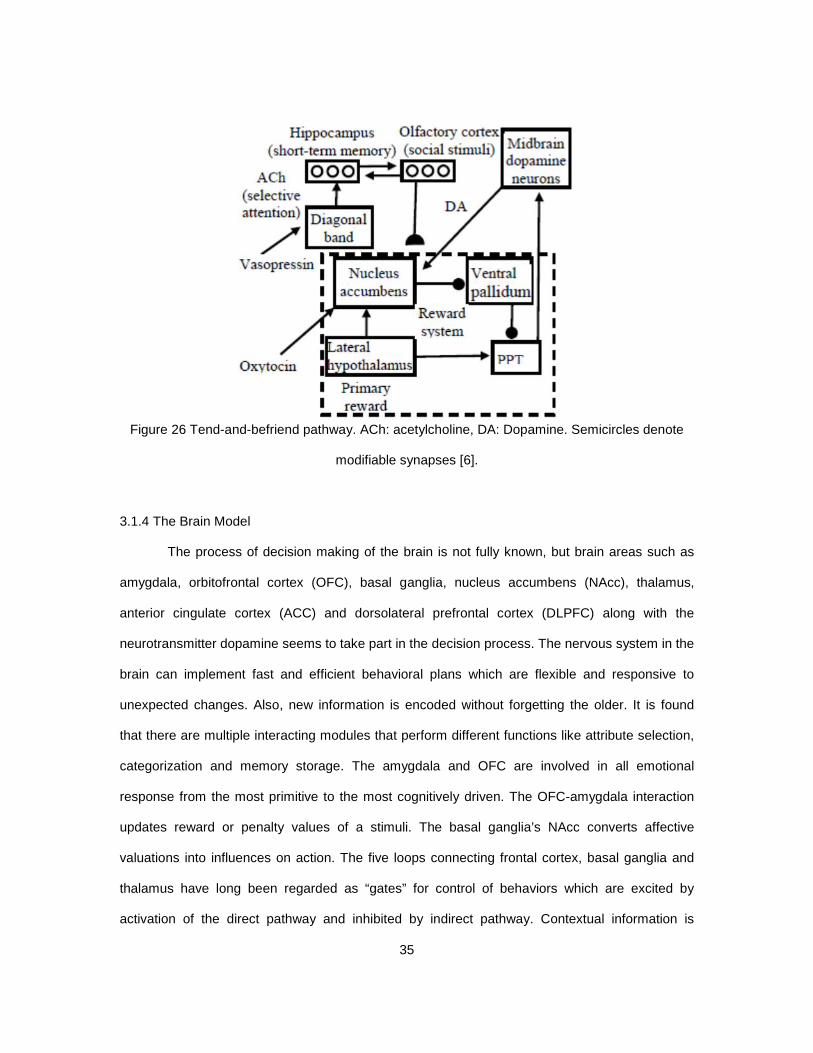
Figure 26 Tend-and-befriend pathway. ACh: acetylcholine, DA: Dopamine. Semicircles denote
modifiable synapses [6].
3.1.4 The Brain Model
The process of decision making of the brain is not fully known, but brain areas such as
amygdala, orbitofrontal cortex (OFC), basal ganglia, nucleus accumbens (NAcc), thalamus,
anterior cingulate cortex (ACC) and dorsolateral prefrontal cortex (DLPFC) along with the
neurotransmitter dopamine seems to take part in the decision process. The nervous system in the
brain can implement fast and efficient behavioral plans which are flexible and responsive to
unexpected changes. Also, new information is encoded without forgetting the older. It is found
that there are multiple interacting modules that perform different functions like attribute selection,
categorization and memory storage. The amygdala and OFC are involved in all emotional
response from the most primitive to the most cognitively driven. The OFC-amygdala interaction
updates reward or penalty values of a stimuli. The basal ganglia’s NAcc converts affective
valuations into influences on action. The five loops connecting frontal cortex, basal ganglia and
thalamus have long been regarded as “gates” for control of behaviors which are excited by
activation of the direct pathway and inhibited by indirect pathway. Contextual information is

36
provided by hippocampus [3] The ACC is activated when there is a conflict about selection of
rules that would govern choices. If higher deliberation and/or low emotional influence is required,
ACC activates DLPFC. DLPFC weighs task relevant attributes more heavily and decreases the
irrelevant, emotional attributes. Thalamus has been found to play role in selective attention
toward attributes [5]. All this has led to three frameworks which together model the decision
process: (1) Gated Dipole Network (2) Adaptive Resonance Theory (ART) (3) Fuzzy Trace
Theory (FTT).
3.1.4.1 Gated Dipole Network
Grossberg (1972) proposed a neural network mechanism that involves two pathways of
antagonistic values as shown in figure 27. The pathways can be thought of as ‘positive’ and
‘negative’ or ‘on’ and off’. Deactivation of an input to one channel leads to transient activation of
the other channel and vice versa. In the figure, J is an input, I nonspecific arousal, w1 and w2 are
synapses and ‘xi’s are activity nodes. When J is on, then x5 is activated even with depleted w1.
After J is shut off and w1 is depleted while w2 does not, x4 becomes more active than x3. This
results in activation of x6 and inhibition of x5.By competition, x6 is activated. If no input J is
present and both w1 and w2 have same potential, there is no effect [1].
Figure 27 Schematic Gated Dipole. ‘->’ denote excitation, • denote inhibition and partially filled
square denote depletion [1].

37
3.1.4.2 Combining Fuzzy Trace Theory and Adaptive Resonance Theory
The ART is essentially a theory of attribute selection and categorization in multilevel
networks. A basic ART network comprises of two interconnected layers of nodes F1 and F2. A
network proposed by Daniel Levine’s which utilizes the ART network is shown in figure 28 with F1
as amygdala and F2 as OFC. F1 and F2, both contain fields of gated diploes. The nodes at F1
represent different attributes of the input (gist encoding) and the nodes at F2 represents different
categories of a particular attribute node at F1. Similar to the amygdala-OFC connections, the
synaptic connections between F1 and F2 are bidirectional and modifiable [5]. These two layers
only classify options of choices with emotional influence. Now, to make choices out of these
options, this ART network is connected with another network which involves ACC for action
selection, basal ganglia and thalamus for action gating and premotor cortex for execution of
action. All of these parts have their local representations of actual options [4]. If there is a match
between the input pattern and wining category, then corresponding action is executed with
positive feedback using direct pathway. If it is a mismatch, then a “reset” is activated by the ACC
and the input is classified into a new category. A parameter called ‘vigilance’ is used for matching
[5].

38
Figure 28 Daniel Levine’s network. -> denote excitation, • denote inhibition and partially filled
square denote depletion [4].
When input Ik has the attention, where I1 = A and I2 = B, the activities of the input nodes
1ix and 1ix in the ith amygdalar attribute dipole, i=1, 2, 3, satisfy the equations [4]
11 3 2 .5ii i i
dxx J bx k R
dt
(3.1.1)

39
11 3 2 .5ii i
dxx bx k R
dt
(3.1.2)
where iJ denotes the ith attribute component of the input vector, denotes non-specific arousal
with 2-.5k factor due to 1.5 times higher arousal, R denotes the activity of the reset node and b is
the decay proportional activity, and output nodes 3ix and 3ix . The depletable transmitter weights
iz and iz have the following dynamics [4]
1(1 )ii i i
dzz x z
dt
(3.1.3)
1(1 )ii i i
dzz x z
dt
(3.1.4)
The node activity equations at the next level of the attribute dipoles are [4]
22 1
ii i i
dxx x z
dt
(3.1.5)
22 1
ii i i
dxx x z
dt
(3.1.6)
The node activity equations at the dipole output layer are [4]
53
3 3 2 3 3 21
(1 )ii i i j ji i i
j
dxx x x y w x x
dt
(3.1.7)
33 3 2 3 2(1 )i
i i i i i
dxx x x x x
dt
(3.1.8)
where jy denotes activity of the jth category node and jiw denotes the weight of the connection
between the jth 3y category node and the 3x node corresponding to the ith attribute. The F2
layer has similar activity and transmitter weight equations for the category dipoles, with 1 jy and
1 jy being input nodes, j and j depletable transmitters, 2 jy and 2 jy layer-2 nodes, and
3 jy and 3 jy output nodes for j=1,…,5 [4].
The weights are solved for the following equation [4],
40
23 3(( ) )( )ji
j ji i
dwy w x
dt (3.1.9)
The reset node activity is defined by [4]
5
1min (j)
j
dRR MATCH
dt (3.1.10)
where MATCH(j) is a measure of closeness between the normalized weight and input vectors [4]:
3 2
1
( ) ki ji ii
MATCH j m NORMWTS NORMINPUT
(3.1.11)
where
3 2
1
jiji
jmm
wNORMWTS
w
,
3
2
1
ii
mm
INORMINPUT
I
and
K: Input corresponding to the planning node activity.
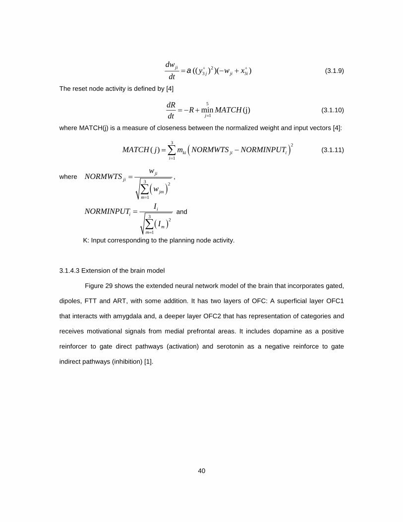
3.1.4.3 Extension of the brain model
Figure 29 shows the extended neural network model of the brain that incorporates gated,
dipoles, FTT and ART, with some addition. It has two layers of OFC: A superficial layer OFC1
that interacts with amygdala and, a deeper layer OFC2 that has representation of categories and
receives motivational signals from medial prefrontal areas. It includes dopamine as a positive
reinforcer to gate direct pathways (activation) and serotonin as a negative reinforce to gate
indirect pathways (inhibition) [1].

41
Figure 29 Neural Network Model of Brain [1]

42
References
1. Daniel S. Levine, “Emotion and Decision Making: Short-term Reactions versus Long-term
Evaluations”, International Joint Conference on Neural Networks, 2006, pp. 195-202.
2. Daniel S. Levine, Leonid I. Perlovsky, “A Network Model of Rational versus Irrational
Choices on a Probability Maximization Task”, IJCNN, 2008, pp 2820-2824.
3. Daniel S. Levine, Britain Mills, Steven Estrada, “Modeling Emotional Influences on
Human Decision Making under Risk”, IJCNN Special Session, Vol. 3, 2005, pp. 1657-1662.
4. Daniel S. Levine, “Neural Dynamics of Affect, Gist, Probability, and Choice”, Cognitive
System Research, Science-Direct, 2012, pp. 57-72.
5. Daniel S. Levine, P. Ramirez, “An Attentional Theory of Emotional Influences on Risky
Decisions”, Progress in Brain Research, Vol. 202, Elsevier (Book), 2013.
6. Daniel S. Levine, “Modeling the Evolution of Decision Rules in the Human Brain”,
International Joint Conference on Neural Networks, 2006, pp. 625-631.
7. Daniel S. Levine, “Seek Simplicity and Distrust it: Knowledge Maximization versus Effort
Minimization”, Plenary talk (PPT), KIMAS, 2007.

43
3.2 Third Generation Brain like Intelligence and Approximate Dynamic Programming
Equation Chapter 3 Section 2
The second section of the second chapter discussed the first and second generation
models of the brain prescribed by Paul Werbos. In this section, a third generation model of the
brain is discussed from his work [1]. He partly agreed with artificial intelligence researchers like
Albus that the human brain has highly complex hierarchical structures to handle a high degree of
complexity in space and in time, because faster learning can be achieved with modified Bellman
equations which use the hierarchical partitioned state space. Though this idea of hierarchy is not
supported by new biological data, there is hypotheses of some kind of specific mechanisms in
three core areas: (1) a “creativity/imagination” mechanism that deals with the complex, non-
convex optimization problem, (2) a mechanism to take care of equations coping with multiple time
scale decisions (3) a mechanism to handle spatial complexity. So he proposed a Strawman
model of the creativity mechanism in 1997 as shown in figure 30 [1].
Figure 30 Third generation brain model of creativity [1]
Yet, much progress is to be made to have brain-like stochastic search. One reason for it
is the association of temporal complexity with spatial complexity. Guyon at AT&T had developed

44
the most accurate ZIP code digit recognizer that utilized spatial symmetry with the help of
modified multilayer perceptron network (MLP), though it could not segment an entire ZIP code
because of failure to handle connectedness. Pang and Werbos (1994) proposed a network called
“Cellular SRN'' (CSRN), integrating the key capabilities of a Simultaneous Recurrent Network and
a “conformal'' network. Unlike MLP, it could learn to predict, control and navigate through far
more complex planes. One of the reasons it could not be used widely is availability of fast
learning tools. Then, however, Ilin, Kozma and Werbos (2008) reported a very fast learning tool
[1].
In 1997 and subsequently, Werbos proposed an approach to exploit symmetry called the
ObjectNet. Here, a complex input field is mapped into a network of k types of “objects” which
have inner loops of k different types. This is the opposite of mapping inputs into M rectangular
cells governed by a common inner loop neural network. Without any assistance from human and
without using a supercomputer, a simple computer system having a simple ObjectNet, which was
designed by David Fogel could achieve master class performance [1].
A brain-like ability is needed to be achieved that can learn more complex transformations
than simple two-dimensional transformations. The CSRN may be exploited for this. But, the first
problem here is to learn symmetries that is, to learn a family of vector maps af such that [1]
( ( 1)) ( 1)Pr Pr
( ( )) ( )
f t t
f t t
x xx x
(3.2.1)
for all and the same conditional probability distribution Pr. This concept is called stochastic
invariance. In simple words, the probability of observing ( 1)t x after observing ( )tx should be
the same as the probability of observing the transformed version of ( 1)t x after observing the
transformed version of ( )tx . These symmetries can be exploited in one of the following ways
once learned [1]:
45
1. “Reverberatory generalization'': after observing or remembering a pair of data
( 1), ( )t tx x , also train on ( ( 1)), ( ( )) .f t f t x x
2. “Multiple gating'': after inputting ( )tx , pick so as to use f to map ( )tx into
some canonical form, and learn a universal predictor form canonical forms.
3. “Multimodular gating'': similar to multiple gating, except that multiple parallel
copies of the canonical mapping are used in parallel to process more than one
subimage at a time in a powerful way.
In 1992, a new architecture called “Stochastic Encoder/Decoder Predictor” (SEDP) was
proposed which extends the ObjectNet theory. SEDP directly learns condensed mappings wit
symmetry relations. It can be thought as an adaptive nonlinear generalization of Kalman filtering.
It still requires methods to speed up the learning process [1].
3.2.1 Stochastic Encoder/Decoder Predictor
As discussed in [2], a stochastic model can be defined by,
ˆ( 1) ( 1) ( 1)i i i iX t X t e t (3.2.2)
where ie represents random noise of unit variance and 2i represents the variance of the error
in predicting iX . Yet, equation (3.2.2) is not a general stochastic model. It assumes that the
matrix Tee is diagonal, and the observed variables always follows a normal distribution. Then,
Werbos suggested that we consider a more general model that may be written as:
( 1) ( 1) ( (t 1), information(t))X Xi i i iX t e t D R (3.2.3)
( 1) ( 1) (information(t))i i i it e t P R RR (3.2.4)
where X is observed and R is not; R is the estimate of the state vector, D stands for “Decoder”
and P for “Predictor”. This can produce any pattern of noise. The problem is adaption of the
networks D and P when R is unknown. The classical likelihood function for this problem involves

46
performing a Monte Carlo integration/simulation based on equations (3.2.3) and (3.2.4), which is
very inefficient. This section will discuss a more efficient design [2].
The Stochastic Encoder/Decoder Predictor design is illustrated in figure 31. It is assumed
that iX equals ˆiX plus some Gaussian white noise. First, information is provided from time
1t into the Predictor network, and the Predictor network calculates ˆ ( ).tR Then, the Encoder
network inputs (t),X along with any information available from time 1t . The output of the
Encoder network is a vector R , a kind of a prediction of the true value of R . Next, generate
simulated values of R , R are generated by adding random numbers to each component iR .
Finally, the Decoder network generates a prediction of X from the R , along with information
from time t -1. These calculations varies according to the weights of Encoder, Decoder, and
Predictor networks, and according to the estimates of i R and .i X [2]
Figure 31 The SEDP [2]

47
3.2.1.1 Adaption of the System
It is difficult to adapt the Encoder network. All parts of the network are adapted together
to minimize [2]:
2 22
2 2 2
ˆ ˆ( (x, , e )) / ( )
log( ) ( ) log( )
Xi i i j j
i j
Xi j j
i j
E X X R R
R R
R R
R
(3.2.5)
This requires the use of backpropagation-gradient based learning to adapt the Encoder
and the parameter i R . The calculated gradients feed the prediction errors back used for
adaption as shown by the dashed line in figure 31. For the encoder, the relevant derivative of E
with respect to jR is [2]:
ˆ ˆ_R 2(R ) _j j j jF R F R (3.2.6)
where the first term results by differentiating the R-prediction error in equation (3.2.5) with respect
to iR and the second term represents the derivative of the X-prediction error which is computed
by back-propagation through the Decoder network back to jR . The Encoder network is adapted
by propagating the _F R derivatives back through the Encoder network. The resulting R from
equations (3.2.5) and (3.2.6) is both predictable from the past and useful in reconstructing the
observed variables iX . If the Predictor network is deleted which results in kind of feature
extractor, then the variance of R has to be minimized to prevent a kind of indirect bias or
divergence from sneaking in. For a similar purpose, the parameters 2j R are adapted based
on [2]:
2 2
2 2_ logj j j j
j j
EF R e
R R
R R(3.2.7)
The networks are adapted by using some information calculated at time t-1 along with back-
propagating the derivatives of equation (3.2.5) to the information producing network [2].

48
Figure 32 shows a block diagram of various parts of the brain which are involved in
decision process. It is based on discussions of the second and third chapters.
Figure 32 Summary of Human Nervous System

49
References
1. Paul J. Werbos, “Intelligence in the brain: A theory of how it works and how to build it”,
Neural Networks 22, 2009, pp. 200-212.
2. Paul J. Werbos, “Handbook of Intelligent Control: Neural, Fuzzy and Adaptive
Approaches”, VAN NOSTRAND REINHOLD, 1992, pp. 493-525.

50
3.3 Cognitive Development with a Psychological Perspective
3.3.1 Introduction
This section talks about studies done similar to Daniel Levine’s to understand the
decision process of the human brain. It includes rule process used for decision [2], types of the
rules and decisions made under risk [1]. Also Piaget’s theory of cognitive development is
explained [3, 4].
3.3.2 Decision Making with Rules
Jansen, Duijvenvoorde and Huizenga in [2] mainly worked in order to outline the
trajectory of integrative versus sequential rule use in decision making. People make decisions
using basically two kinds of rules: (1) Sequential rules in which decision is made by evaluating
dimensions of choices sequentially. (2) The integrative normative rule in which decisions are
made by integrating the choice dimensions. In case of the sequential rule, a particular dimension
is chosen and options are compared based only on this dimension. A decision is reached if
options are different on this dimension; otherwise another dimension is considered. So,
dimensions are processed one by one and not integrated like multiplication of two dimensions.
Jansen and the others [2] administered the Gambling Machine Task (GMT) to spanning a
broad age range of people. They collected data based on the rules used for decision and number
of dimensions used for the rules. Figure 33 shows results of their experiment. It can be observed
that use of integrative rule decreases and use of sequential rule increases with increase in the
age which contradicts proportional reasoning theory and supports fuzzy trace theory. Also, it can
be observed that number of dimensions considered increase with increase in age which supports
the proportional reasoning theory. Faster and less effortful decisions can be made by using the
sequential rule as compared to using integrative rule, but it may sometimes lead to wrong
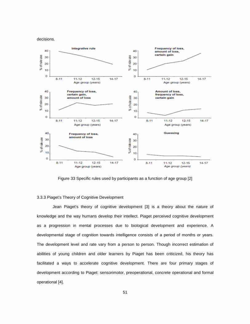
51
decisions.
Figure 33 Specific rules used by participants as a function of age group [2]
3.3.3 Piaget’s Theory of Cognitive Development
Jean Piaget’s theory of cognitive development [3] is a theory about the nature of
knowledge and the way humans develop their intellect. Piaget perceived cognitive development
as a progression in mental processes due to biological development and experience. A
developmental stage of cognition towards intelligence consists of a period of months or years.
The development level and rate vary from a person to person. Though incorrect estimation of
abilities of young children and older learners by Piaget has been criticized, his theory has
facilitated a ways to accelerate cognitive development. There are four primary stages of
development according to Piaget: sensorimotor, preoperational, concrete operational and formal
operational [4].

52
3.3.3.1 Sensorimotor Stage
First stage in cognitive development is the sensorimotor stage. It spans from birth until
the acquisition of language (till the age of 2 years). Object permanence is one of the most
important aspect of this stage in which the child understands that objects can exist whether they
can be seen, heard, touched or not. It has been found that children can link numbers and
counting to the objects. [4] Of course, children learn to control and coordinate their senses and
motor actions [3].
3.3.3.2. Preoperational Stage
The preoperational stage starts when the child begins to speak at the age of 2 and lasts
until the age of 7. The child’s language ability increases in this stage. The child can perceive and
represent symbols related with objects. The child has a little logic and cannot perceive from more
than one viewpoint [3, 4]. For example, when same amount of liquid from one container is
transferred to another container with less height, the child thinks that amount of liquid has
decreased in the later container [4].
3.3.3.3 Concrete Operational Stage
This third stage occurs generally between the age of 7 and 11. The child undergoes a
remarkable cognitive growth. In the child, Language development and basic skill acquisition
accelerate dramatically. Children at this stage can now perceive other viewpoints, can consider
two or three dimensions simultaneously. They can classify objects based on a common
characteristic like number, mass and weight. The classification can also be done in ascending or
descending order. They are now able to think logically, can reverse an operation-can perform
addition and subtraction. [3, 4].

53
3.3.3.4 Formal Operational Stage
This the fourth stage of cognitive development. The children at this stage are capable of
hypothesizing and deduction which is needed in science and mathematics. Abstract thoughts
emerge with logical use of symbols in this stage. The children can identify and analyze elements
of a problem, so that they can decipher the information needed in solving a problem. Additionally,
they can evaluate the adequacy of a problem solution using some criteria. Thus, the children can
relate mathematical concepts to real life situations [4].
3.3.4. Cognition and Decision under Risk
Cokely and Kelley [1] investigated the relationship between cognitive abilities and
superior decision making under risk. Some mechanisms try to provide this link. One way is to
calculate expected value to make expected value choices (Fredrick, 2005). Working memory
capacity (Stanovich and West, 2000) and numeracy – understanding of probabilities (Peters &
Levin, 2008; Peters et al., 2006) may lead to individual differences in the choices in various
conditions. The priority heuristic model of decision hypothesize that decisions between sure and
risky options are made by considering simple reasons in a fixed order until a stopping rule is met.
Then Cokely and Kelley discuss a dual process model which includes priority heuristics and a
simple heuristic processes. It is assumed in this model that controlled cognition relates to more
rule-based, abstract and decontextualized reasoning; while more automatic and impulsive
cognition is relate to associations, personal relevance, and situational contextual information.
In the experiment, they found out that more elaborative heuristic search was performed in
decision making under risk as opposed to expected value calculations which is not a computation
of an answer; but a monitored and corrected output of an automatic process. The priority heuristic
also was proven wrong. Variations in risky choices are linked to differences in duration and type
of information search. Therefore, it is suggested that elaborative heuristic search which involves
more thorough exploration and representation, is related to superior risky decision making which
yields faster and correct reasons most of the time; but not always.. It is not necessary higher

54
performing individuals always search or reflect more. Yet, the decision process is not well
understood [1]

55
References
1. Edward T. Cokely, Colleen M. Kelley, “Cognitive abilities and superior decision making
under risk: A protocol analysis and process model evaluation”, Judgment and Decision Making,
Vol. 4, No. 1, February 2009, pp. 20–33.
2. Brenda R. Jansen, Anna C. Duijvenvoorde, Hilde M. Huizenga, “Development of Decision
Making: Sequential versus integrative rules”, Journal of Experimental Child Psychology 111,
2012, pp. 87-100.
3. Piaget’s theory of cognitive development-from Wikipedia.
4. Bobby Ojose, “Applying Piaget’s Theory of Cognitive Development to Mathematics
Instruction”, The Mathematics Educator, Vol. 18, No. 1, 2008, pp. 26-30.

56
Chapter 4
New Neuro-inspired Architectures for Learning and Control
4.1 Neuro-inspired Networks for Learning
4.1.1 Introduction
Various sections before have discussed about how decision process takes place in the
human brain with biological and psychological findings. Also, a couple of models of the brain were
discussed. This section discusses about various models which were inspired from the decision
process of the brain for learning and control purposes. It includes reinforcement learning ([1] and
[2]), and artificial neural networks ([4] and [5]).
4.1.2 Shunting Inhibitory Artificial Neural Networks
Bouzerdoum [5] proposed biologically inspired Shunting Inhibitory Artificial Neural
Networks (SIANNs) in which a nonlinear shunting inhibition mechanism mediates the synaptic
interactions among neuron. One or more number of hidden layers can have neurons which use
shunting inhibition. The outputs of these hidden layer neurons are linearly combined to form the
output. With help of the inherent nonlinearity, the SIANN is capable of constructing very complex
nonlinear decision boundaries which can be used for classification and function approximation.
This requires to have an efficient training algorithm. The SIANN has already been used
successfully as adaptive filters and for pattern recognition.
4.1.2.1 Definition of SIANN
The dynamics of a feedback shunting inhibitory neural network can be described as
follows [5]:
ii i i ij j i i
j
dxI a x f c x x b
dt
(4.1.1)

57
where ix is the activity of the ith neuron; Ii is the external excitatory input; ia is a positive
constant representing the passive decay rate of the neuron activity; ijc is the connection weight
from the jth neuron to the ith neuron; bi is a constant bias; and f is a positive activation function.
The external inhibitory input Ij replaces he activation of the jth neuron, jx in feedforward
network which has the following dynamics [5]:
ii i i ij j i i
j
dxI a x f c I x b
dt
(4.1.2)
The steady-state response of the feed-forward network is given by [5],
i ii
i ij jj
I bx
a f c I
(4.1.3)
Figure 34 Steady state model of a shunting neuron [4]
The final output y linearly combines the outputs of the shunting neurons through an
activation function g [5],
i ii
y g w x b
(4.1.4)
where iw is a connection weight and b is a bias term. Figure 35 shows an SIANN with m inputs,
one hidden layer and n outputs.

58
Figure 35 Feedforward SIANN [4]
4.1.2.2 Decision Regions of SIANN
Let us consider a simple SIANN with two neurons in the shunting (hidden) layer. The
activations of the shunting neurons are [5],
1 1 2 2
1 21 11 1 12 2 2 21 1 22 2
,I b I b
x xa f c I c I a f c I c I
(4.1.5)
and the output of the SIANN is [5],
1 1 2 2(w )y g x w x b (4.1.6)
The decision boundary of this network is given by [5],
1 1 2 2w 0x w x b (4.1.7)
Now, quadratic decision boundaries can be constructed by selecting a linear activation
function. A nonlinear activation function would construct more complex decision surfaces. Figure
36 illustrates the decision regions of the above mentioned SIANN with the logistic activation
function ( ) 1/ (1 )xf x e .

59
Figure 36 Decision regions of SIANN. a1=a2=1, b1=b2=5, w1=-2, w2=2, c12=c21=1, c11=c22=5
[4].
The shunting layer does a nonlinear transformation on the inputs form a pattern such that
it classifies easily with a discriminant function [4].
4.1.2.3 Training SIANN
To produce desired outputs for given inputs, a neural network has to be trained to find
appropriate connection weights. The backpropagation is a widely used algorithm for training
MLPs in which weights are updated that minimizes the mean-square error along with the use of
differentiable activation function. This method can be adapted to train SIANNs. For an SIANN
with a single output neuron, the squared error can be defined as [5],
221 1
2 2E e y d (4.1.8)
where, d is the desired output, y is the actual output and e is the error.
The gradient of the squared error E with respect to the parameter ijc is [5]

60
i j ij jji
iij i ij
i ij jj
x I f c IxE E
c x ca f c I
(4.1.9)
with i ii i
E E yw g e
x y x
where i is the backpropagated error signal and the prime represents differentiation with respect
to the argument. Similarly, partial derivatives of E with respect to ia , ib , iw and b can be
derived. In the gradient descent algorithm, a network parameter can be updated as in [5],
new old
E
(4.1.10)
where is the learning rate and is one of the network parameters [4].
4.1.2.4 SIANN versus MLP
Figure 37 displays the performances of SIANN and MLP where the function to be
approximated is 2( ) 0.1 1.2 2.8 sin(4 )h t t t t , [0,1]t . It can be seen that the SIANN
approximates the function more accurately than the MLP.
Figure 37 Estimated function using SIANN and MLP [4]
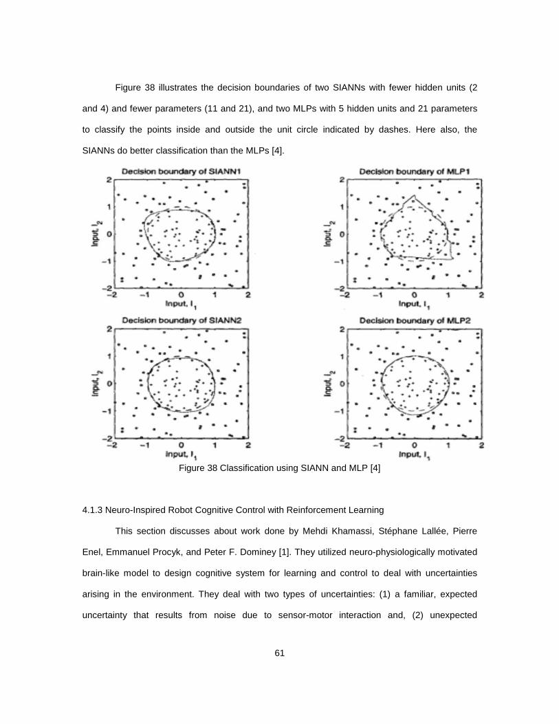
61
Figure 38 illustrates the decision boundaries of two SIANNs with fewer hidden units (2
and 4) and fewer parameters (11 and 21), and two MLPs with 5 hidden units and 21 parameters
to classify the points inside and outside the unit circle indicated by dashes. Here also, the
SIANNs do better classification than the MLPs [4].
Figure 38 Classification using SIANN and MLP [4]
4.1.3 Neuro-Inspired Robot Cognitive Control with Reinforcement Learning
This section discusses about work done by Mehdi Khamassi, Stéphane Lallée, Pierre
Enel, Emmanuel Procyk, and Peter F. Dominey [1]. They utilized neuro-physiologically motivated
brain-like model to design cognitive system for learning and control to deal with uncertainties
arising in the environment. They deal with two types of uncertainties: (1) a familiar, expected
uncertainty that results from noise due to sensor-motor interaction and, (2) unexpected

62
uncertainty that results from varying stochastic environment. The model could deal with these
uncertainties by adaptively regulating a meta-parameter called .
4.1.3.1 Experiment Setup
A humanoid agent–a physical robot or a simulation is considered in the experiments done
in [1]. The interaction with the environment is done through visual perception and motor
commands. All three experiments are similar and use vision systems to provide all the inputs. An
agent has to search by trial and error (exploration) to find the best possible reward. Then the
agent has to repetitively select the best award which is exploitation. Indication of new exploration
task is provided by a problem-changing cue (PCC). The agent has to learn to decide probability
and the PCC in the experiments.
4.1.3.2 The Neural Network Model
In the work done by Khamassi and the others [1], the neural network model whose
architecture is inspired by anatomical connections in the brain of the monkeys is shown in figure
39. The locations in the visual space are encoded by a 3 * 3 array of leaky integrator neurons. A
neuron’s membrane potential mp is given by [1]:
mpmp s
t
(4.1.11)
where is a time constant and s is input. Then average firing rate output based on a nonlinear
function is generated. The posterior (PPC) receives the visual input. The ACC estimates action
values associated with each possible selections based on temporal difference algorithm. This
action values are sent to dopamine neurons in the ventral tegmental area (VTA) where a reward
prediction error is computed after reception of the reward [1]:
(a )ir Q (4.1.12)
where ai, i [1,…, 4] is the action value and r is the reward value. The reinforcement signal is
sent to ACC to update the weights corresponding to the action value neuron [1]:

63
( ) ( ) ( )i i iQ a Q a trace a (4.1.13)
where trace is the efferent copy of the chosen action sent by the premotor cortex (PMC) to
reinforce the ACC and is a learning rate.
Figure 39 The neural model [1]
Now, an outcome history (COR-correct neuron; ERR- error neuron) is computed
modulate the exploration level *ß in ACC [1]:
( ) ( ), ( ) 0COR t t if t ( ) ( ), ( ) 0ERR t t if t
( ) ( ) ( ) (t)t t COR t ERR (4.1.14)

64
where 2.5 and 0.25 are updating rates with * (0< *<1). The ACC sends
action values * to DLPFC. The DLPFC regulates the exploration rate (0 10) by a
sigmoid function with sign reversal [1]:
1
2 3(1 exp( [1 ] ))
(4.1.15)
where 1 =10, 2 6 and 3 1 . The DLPFC decides upon the action to be taken based on a
Boltzman softmax function [1]:
exp( ( ))( )
exp( ( ))i
ij
j
Q aP a
Q a
(4.1.16)
where 0< regulates the exploration rate. A small leads to exploration as each action has
almost equal probabilities where as a high leads to exploitation. The selected action to be
executed is gated through the cortico-basal ganglia loop consisting of striatum, substantia nigra
reticulata (SNr), and thalamus (Thal) until the premotor cortex (PMC). The PMC is used to
command the agent.
The ACC learns association of average reward with different objects using meta-values
and they are updated with dependence on the variations in the average reward at the end of each
trial [1]:
( , ) ( , ) ( )i iM o t M o t t (4.1.17)
where is learning rate and ( )t is the estimated reward average. If the meta-value of any
object is lower than a threshold, then action values are reset to some random values and * is
increased. This means a low and the agent will start exploration instead of doing exploitation.

65
References
1. Mehdi Khamassi, Stéphane Lallée, Pierre Enel, Emmanuel Procyk, Peter F. Dominey,
“Robot cognitive control with a neuro-physiologically inspired reinforcement learning model”,
Frontiers in Neurorobotics, volume 5, article 1, 2011, pp. 1-14.
2. Christian Balkenius, Stefan Winberg, “Cognitive Modeling with Context Sensitive
Reinforcement Learning”, Proceedings of AILS 04, 2004, pp. 10-19.
3. Petru E. Stingu, Frank L. Lewis, “Neuro Fuzzy Control of Autonomous Robotics”,
Springer (Book), 2009.
4. Ganesh Arulampalam, Abdesselam Bouzerdoum, “A generalized feedforward neural
network architecture for classification and regression”, Neural Networks 16, 2003, pp. 561–568.
5. Abdesselam Bouzerdoum, “Classification and function approximation using feed-forward
shunting inhibitory artificial neural networks”, IJCNN, 2000, pp. 613-618.
6. Joshua Brown, Daniel Bullock, Stephen Grossberg, “How the basal ganglia use parallel
excitatory and inhibitory learning pathways to selectively respond to unexpected rewarding cues”,
The Journal of Neuroscience, 1999, pp. 10502–10511.

66
4.2 Multiple Model Based Learning and Control
4.2.1 Introduction
Previous section discussed various controllers inspired from the study of the decision
process done by the human brain. They all used single controller/predictor to achieve a particular
goal. But, further study of brain suggests that are multiple control structures working
simultaneously in the brain. This has led to use of multiple controllers and/or predictors used.
Here, some of them are discussed which use multiple reinforcement learning structures, multiple
neural networks and multiple adaptive controllers.
4.2.2 Multi-Model Adaptive Control
This section discusses the work done by Narendra and Balakrishnan in [5]. They believed
that an intelligent controller needs to have the ability to adapt rapidly in any unknown, rapidly
changing environment. To serve this purpose, they proposed different switching and tuning
schemes for multiple model adaptive control. It combines fixed and adaptive models in various
ways. They have studied this multiple model architecture with all fixed models, all adaptive
models and one adaptive-rest fixed models. These schemes are proved to be stable. When the
environment of a system changes abruptly, a new model of the environment along with the
appropriate controller has to be chosen other than the current one. The controllers can be pre-
designed if the models are already available for different environments. As there are only finite
number of models with any possible environment, switching and tuning are very important. The
switching is to select the model matching with some defined criteria rapidly. The tuning is the
adjustment of the parameters of the chosen model tom improve accuracy. It is difficult to decide
the moment of switch, which model and the rule to be used for tuning.
4.2.2.2 Design of the Control System
The proposed architecture by Narendra and Balakrishnan [5] for intelligent control is
shown in figure 40. This is a general one and can be applied to both linear and nonlinear

67
systems. The system to be controlled has input u and output y . The aim is to make the control
error ce y y go to zero, where *y is the desired output. There are N identification models
which are denoted by 1
N
j jI
operate in parallel. ˆ jp is the parameter vector of each jI . The
identification error between the output jy of jI and that of the plant is denoted as ˆj je y y .
There is a controller jC corresponding to each jI , which has parameter vector j . The output of
jC is denoted by ju . One jI is selected by a switching rule and the corresponding control input
ju controls the plant. The design problem here is to select the number of models and controllers
along with their parameters. The control problem is to decide the rules for switching and tuning
that can give a stable and the best performance.
Figure 40 A multi-model architecture [5]

68
4.2.2.3 Switching Rule Selection
Narendra and Balakrishnan have presented methods to select switching rule in [5]. One
way is to compute performance cost indexes ( )iJ t corresponding to every controller jC at every
moment and then switching to the one with the minimum index; but this requires to apply all the
control inputs which is not possible. So, a feasible option of simultaneous computation of
performance indexes of all the identification models is used, which means that identification
errors je are used. The performance index can be computed as [5],
2 ( ) 2
0
( ) ( ) ( ) , 0, , 0t
ti j jJ t e t e e d (4.2.1)
where and are utilized for desired combination of instantaneous and long-term accuracy
measures, is the forgetting factor from which the memory of the index is decided and it is an
assurance of boundedness of (t)iJ for bounded je . A minimum wait period is allowed to elapse
after every switch in order to prevent arbitrarily fast switching.
4.2.3 Multiple Model-Based Reinforcement Learning
Kenji Doya and the others [1, 2] proposed a multiple model based reinforcement learning
(MMRL) architecture for nonlinear, non-stationary control tasks. It has a modular architecture of
multiple models. Basically, a complex task is divided into multiple domains in space and time. It
can learn all possible outcomes resulting from a same cue stimulus. Additionally, this multiple
model architecture has provided a valid explanation of the behavior of dopamine neurons in
reward prediction. An implementation of the MMRL is shown in the figure 41. Every module has a
reward predictor and a value estimator. After the cue stimulus, the model predicts the presence or
absence of reward at each time step. A vector of the predicted amount of reward is given by each
reward predictor. A responsibility signal λi corresponding to the each module is calculated based
on the prediction errors of the reward predictors. The reward predictors and value estimators are

69
updated by gating the responsibility signal. Also, it is used to weight the output of the value
estimators. This architecture can be used for control as extended in [1] and it is called modular
selection and identification for control (MOSAIC).
Figure 41 The MMRL architecture [2]
Let us understand how this model works: Assuming there are N > 2 modules, an MMRL
has previously trained two reward predictors 1 and 2, predicting a Stimulus-Reward Interval (SRI)
of t1 and t2 respectively, with t1 < t2. These to modules predict an amount of reward depending
on the previous training at t1 and t2. If the current time t elapsed since the stimulus occurred is
small (t < t1 < t2), they both have high responsibility with likely prediction. If no reward occurs at
t=t1, then the first predictor makes a large prediction error and its responsibility is downgraded.
So, while t1 < t < t2, the overall prediction will mostly depend on second predictor. If at t = t2 no

70
reward occurs, the predictor 2 will also have a large error and then low responsibility. If a reward
occurs afterwards, the most likely of the rest of the predictors will have the highest responsibility
[2].
4.2.3.1 Reward Predictor
The reward predictor r (t) of each module i gives a vector of the predicted reward. The
responsibility signal for each predictor is computed as [2]:
2
2
2
2
( )
2
( )
2
ˆ ( )( )
ˆ ( )
i
j
E t
ii E t
jj
t et
t e
(4.2.2)
where is a constant and ˆ( ) ( ) ( )i iE t r t r t the prediction error of each reward predictor,
( )r t is the actual amount of reward at time step t and ˆ ( )i t is the estimated responsibility value
encoding some prior knowledge. If the temporal continuity of module selection is considered as
the prior knowledge, then using the previous responsibility [2]:
ˆ ( ) ( 1)i it t (4.2.3)
where 0 1 a parameter that controls the strength of the memory effect. Each reward
predictor ˆ ( )ir t is initialized to random values and is updated according to the following equation
[2]:
ˆ ˆ( ) ( ) ( )i i i ir t r t E t (4.2.4)
with 0 1 an update rate.
4.2.3.2 Value Estimator
The value estimator of each module updates values similarly to a tap delay line model [2]:
( ) ( ) ( )i iV t s t w t (4.2.5)

71
where iw is a weight row vector. The global predicted value signal ( )V t is a weighted sum of
the modules’ values [2]:
( ) ( )i ii
V t V t (4.2.6)
The Temporal Difference (TD) error ( )t is [2]:
( ) ( ) ( 1) ( )t r t V t V t (4.2.7)
where 0 1 is discounting parameter. The TD error for each module is gated by [2]:
( ) ( )i it t (4.2.8)
The weight vector of each value estimator is updated by [2]:
( ) ( ) ( ) ( )i i iw t w t s t t (4.2.9)
with learning rate .
4.2.4 Extended Modular Selection and Identification for Control
4.2.4.1 Introduction
Norikazu Sugimoto, Jun Morimoto, Sang-Ho Hyon, and Mitsuo Kawato in [6] present an
extension of the MOSAIC architecture for humanoid robot control. A MOSAIC architecture is
proposed by Doya and the others in [1]. Also, another is proposed consisting of multiple linear
state predictors and controllers. The MOSAIC architecture is flexible enough to learn and control
the nonlinear and non-stationary environment. Still, it has the limitations of susceptibility to
observation noise and requirement of fully observable system. The eMOSAIC architecture
includes state estimators to cope with these two problems in a real environment. This inclusion of
the state estimators can better explain the sensorimotor function of the central nervous system.
The authors of this work successfully generated squatting and object-carrying with a real
humanoid robot.

72
4.2.4.2 The eMOSAIC Model
Figure 42 shows the eMOSAIC model proposed by Norikazu Sugimoto, Jun Morimoto,
Sang-Ho Hyon, and Mitsuo Kawato in [6]. Each module consists of a state estimator, a
responsibility predictor, a value function estimator, and a controller. They used switching of linear
models and quadratic models to estimate nonlinear states and nonlinear cost function,
respectively. The dynamics are [6]:
( 1) ( ) ( ) ( ),i i it A t B t c t x x u n (4.2.10)
( ) ( ) ( )it H t t y x v (4.2.11)
1 1( ( ), ( )) ( ) ( ) ( ) ( )
2 2T T
i i ir t t t Q t t R t x u x x u u (4.2.12)
where N NiA R and N D
iB R are regression parameters of the ith linear dynamics, Nic R
is bias parameter, and L NiH R is an observation matrix. , RN DR x u and LRy are
state, action and observation vectors, respectively, and ( ) (0, )t N xn and ( ) (0, )yt N v
are system and observation noises. (0, )N denotes a Gaussian distribution with zero mean
and covariance . N NiQ R and D D
iR R are parameters of the ith quadratic cost function ir
. Optimal controller is found by minimizing the objective function [6]:
0
( ( ), ( ))s
J E r s s
x u (4.2.13)
And the objective function is minimized by estimating the value function [6]:
( ( )) ( ( ), ( ))s t
V t E r s s
x x u (4.2.14)
Its working is similar to that of MMRL discussed in the previous section. Each modular
function is discussed in the next sub-sections.

73
Figure 42 The eMOSAIC model [6]
4.2.4.3 Learning Forward Models
The objective is to minimize the weighted prediction error. If each model is represented in
a linear form ( 1) ( ),i it W t x z the expected values for the regression parameters iW can be
derived as [6]:
( )
( )i
i T
i
TW
T
xz
zz(4.2.15)
The notation ( )i
g T annotated a weighted mean of a function g with respect to the
responsibility signal ( ) :i t
1
1(T) ( ) ( )
T
iit
g g t tT
(4.2.16)
The responsibility signal is a probability distribution of the module selection. The
likelihood of the learning of the forward model can be made suboptimal by iterating the
responsibility signal calculation and parameter update.

74
4.2.4.4 State Estimators
A linear state estimator estimates the latent dynamics [6]:
ˆ ˆ( 1| ) ( ) B ( )i i i i it t A t t c x x u (4.2.17)
ˆ ˆ ˆ( 1) ( 1| ) K ( ( ) ( 1| ))i i i i it t t t H t t x x y x (4.2.18)
where ˆ ix is the estimated state and iK is the parameter of the state estimator which can be
found by solving the linear optimal estimation problem.
4.2.4.5 Responsibility Predictors
The probability distribution i weightage of each module and it is given by the Bayes’
rule [6]:
'
( ) ( ( ) | (1: t), i)( )
( ') ( ( ) | (1: t), i')i
i M
P i p tt
P i p t
x yx y
(4.2.19)
where M is the set of module indices, ( ( ) | (1: t), i)p tx y is the likelihood of the ith module, and
( )P i is the error. It is assumed that the prediction error and estimation error are Gaussian with
covariances x and y . So, the likelihood of the ith module ( ( ) | (1: t), i)p tx y is given by [6]
( ( ) | (t), i) ( ( ) | (t | t 1), i) ( ( ) | (t | t 1), i)p t p t p t x y y x x x (4.2.20)
11 1( ( ) | ( | 1), ) exp ( ) ( )
2(2 )
Ti i
Ly
p t t t i t t
yy x e e (4.2.21)
ˆ( ) ( ) ( | 1)i i it t H t t e y x (4.2.22)
11 1
( ( | 1), i) exp ( ) ( )22
Ti iN
p t t t t
x
x
x d d(4.2.23)
( ) ( ) ( 1) ( 1)i i i i i it t A t B t c d x x u (4.2.24)
where ˆ ( | 1)i t t x is the predicted state of the state estimator of the ith module and
ˆ( ) ( ) ( | 1)i i it t H t t e y x is the so called error of innovation.

75
Finally, the estimated state is computed by the weighted sum of each module [6]:
ˆ ˆ( ) ( ) ( )i ii M
t t t
x x (4.2.25)
where ˆ ( )i tx is the estimated state of the ith module at time t.
4.2.4.6 Value Function Estimators
The value function is locally estimated by using a quadratic function [6]:
1 ˆ ˆ( ( )) ( ( ) ) ( ( ) )2
v T vi i i iV t t P t x x x x x (4.2.26)
where the matrix iP is given by solving Riccati equation [6]:
10 T Ti i i i i i i i i iP A A P PB R B P Q (4.2.27)
The center term vix of the ith value function is given by [6],
1( )vi i i i i iQ P A Pc x (4.2.28)
4.2.4.7 Controllers
A linear-quadratic optimal control problem is solved locally to derive the controller. With
the estimated value function in Eq. (4.2.26), linear optimal controller for the ith module can be
derived as [6],
ˆ( ) ( ( ) )T ui i i i it R B P t u x x (4.2.29)
The final output of the controller is computed by the weighted sum of each module output [6]:
( ) ( ) ( )i ii M
t t t
u u (4.2.30)
76
References
1. K. Doya, Kazuyuki Samejima, Ken-ichi Katagiri, Mitsuo Kawato, “Multiple Model-Based
Reinforcement Learning”, Neural Computation, 2002, pp. 1347-1369.
2. Mathieu Bertin, Nicolas Schweighofer, K. Doya, “Multiple model-based reinforcement
learning explains neuronal dopamine activity”, Neural Networks 20, 2007, pp. 668–675.
3. Okihide Hikosaka, Hiroyuki Nakahara, Miya K. Rand, Katsuyuki Sakai, Xiaofeng Lu, Kae
Nakamura, Shigehiro Miyachi, Kenji Doya, “Parallel neural networks for learning sequential
procedures”, TINS Vol. 22, No. 10, 1999, pp. 464-471.
4. Tetsuya Minatohara, Tetsuo Furukawa, “The Self-Organizing Adaptive Controller”,
International Journal of Innovative Computing, Information and Control, Vol 7, number 4, April,
2011, pp. 1933-1947.
5. Kumpati Narendra, Jeyendran Balakrishnan, “Adaptive control using multiple models”,
IEEE TRANSACTIONS ON AUTOMATIC CONTROL, VOL. 42, NO. 2, 1997, pp. 171-187.
6. Norikazu Sugimoto, Jun Morimoto, Sang-Ho Hyon, Mitsuo Kawato, “The eMOSAIC
model for humanoid robot control”, Neural Networks, 2012, pp. 8-19.

77
Chapter 5
Satisficing
5.1 Satisficing and Control
This section introduces a new concept in control theory named ‘satisficing’. It is different
from optimality and even sub-optimality. First, satisficing is explained with respect to various
faculties. Then the focus is put on using satisficing for control theory which involves the work
done by Goodrich [2] and Curtis [3].
5.1.1 What is Satisficing?
Satisficing is a decision making strategy in which the first option is selected that meets an
acceptability threshold out of the available alternatives. This differs from an optimal decision in
which the best option is chosen. The term satisficing can be thought of as combining the two
words satisfy and suffice. The concept was first presented in Administrative behavior in 1947.
Herbert A. Simon introduced satisficing to explain non-optimal decisions made by humans due to
the lack of cognitive resources like limited memory and less knowledge of probabilities of
outcomes [1]. This is related to an approach of bounded rationality which is discussed in the next
chapter.
Let us understand satisficing through an example: The objective to sew a patch onto a
pair of jeans for which a 4 inch long needle with a 3 millimeter eye, is the best-optimal option.
Now, this needle is put in a pile of 1000 other needles varying in size from 1 inch to 6 inches.
Searching for the best needle from this haystack is very effortful and time-consuming. Instead,
using the first needle that can sew on the patch is a satisficing solution. Later on, satisficing may
led to optimization. Satisficing can help to make a an effective and an efficient decision like in the
choice of an outfit; but it may led to wrong decision as in case of medical issues. A person can be
a maximizer (optimizer), a satisficer or something in between [1].

78
A satisficing problem can be defined as an optimization problem using the indicator
function of the satisficing requirements as an objective function. With X denoting the set of all
options and S X denoting the set of "satisficing" options, a satisficing solution from S can be
found by solving the optimization problem [1]:
max ( )Ss X
I s
where SI denotes the indicator function of S , that is
1,( ) : ,
0,S
s SI s s X
s S
A solution s X to this optimization problem is optimal if and only if it is a satisficing
option. Thus, the difference between "optimizing" and "satisficing" is essentially a stylistic issue
rather than a substantive issue. The important thing is to decide whether and what performance
measure should be optimized or satisficed. Jan Odhnoff noted in his paper in 1965 that an
optimal result can be an unsatisfactory result in a satisficing model [1].
Simon and the others suggested the idea of aspiration level which is the payoff that the
agent aspires to. With aspiration level A and maximum payoff U , let s define A ≤ U*. Then,
A: s ∈ S if and only if A ≤ U(s). Also, the set of all options that yield maximum payoff, O ⊆ S
since A ≤ U* [1].
Another way to define satisficing is epsilon-optimization. If the "gap" between the
optimum and the aspiration is ε = U* − A, then the set of satisficing options S(ε) can be defined as
all those options s such that U(s) ≥ U* − ε, that is the actions for which the payoff is within epsilon
of the optimum [1].
5.1.2 Satisficing Decisions
Goodrich, Stirling and Frost discuss a way to use satisficing for decision and control in
[2]. They extend their theory by introducing ‘strong satisficing’ which supports a systematic
79
procedure for a control design. It is then tested for some application yielding comparable results
with optimal control design. Their work adapts from epistemic utility theory. Their approach
involves performance measures and design principles to characterize terminal and transition
costs. Two independently developed utilities, accuracy (benefit-like attribute) and liability (cost-
like attribute), are compared which are defined over the expected consequences of a decision.
Similar to the methodology epistemic utility theory, the goal here is of ‘error avoidance’; not truth
seeking (optimality).
The epistemic utility function is convex and is defined as [2]:
( , ) ( ; ) (1 )(1 P ( ; ))A LG P G G (5.1.1)
where [0,1] , ( ; )AP G is a probability measure of accuracy support associated with G
when is the state of nature, and ( ; )LP G characterizes the liability exposure associated with
G . With a positive linear transformation the utility function is [2]:
( , ) ( ; ) P ( ; ))b A LG P G b G (5.1.2)where (1 ) /b is the index of rejectivity. If the state of nature is viewed as a random
variable and ( )P W represents the belief that W contains the actual state of the nature, then
the expected value of the epistemic utility function is defined as [2]:
( ) ( ; ) ( ; ) ( ) ( ) ( )b A L A LG P G bP G P d P G bP G
(5.1.3)
where (G)AP and (G)LP are expected density function for accuracy and liability, respectively
and have unit mass. Now satisficing is defined in terms of epistemic utility theory. The
equivalence class of sets [2]:
: arg max ( )b bG B
C S B S G
(5.1.4)
which is the family of all measurable sets that maximize expected epistemic utility. If bS is a
member of this equivalence class, then it is known as ‘maximally satisficing set’ for rejectivity b
and if bG S , then G is a satisficing set [2]. In terms of control action u [2]:

80
{ : (u) (u) 0}b A LS u P bP (5.1.5)
This approach does not require a unique best decision; all the decisions are included for which
the above condition is met. Then any one action can be chosen out of this set with the confidence
of achieving a justifiable performance. This satisficing controller is insensitive to time-variance as
it uses only temporally local information.
5.1.3 Constructive Nonlinear Control using Satisficing
J. W. Curtis and R. W. Beard [3] used satisficing to constructively parameterize a class of
universal formulas. They used a control Lyapunov function (CLF) to design satisficing control.
The two functions used for the parameterization are constrained to be locally Lipschitz and satisfy
convex constraints. They give two examples to illustrate the approach. A CLF is a positive
definite, radially unbounded function whose derivate along the system trajectories is negative
definite. The CLF can be easily defined without a need to specify any feedback function for a
systems with inputs; unlike traditional Lyapunov functions. Sontag has shown that by using a
known CLF and the universal formulas, a nonlinear can be rendered to be asymptotically stable
system. Here, the universal formulas are parameterized by using the notion of satisficing decision
theory. The basic idea is to define two utility functions, ‘selectability’ (benefits of choosing an
action) and ‘rejectability’ (cost of choosing an action), that quantify the benefits and costs of an
action. The “satisficing” set is defined to be those options for which selectability exceeds
rejectability. The selectability” function is linked to a CLF [3].
5.1.3.1 Satisficing Set
Curtis and Beard [3] consider an affine nonlinear system
( ) ( )x f x g x u (5.1.6)
where nxR , : n nf R R , g : n n mR R and muR . f and g are locally Lipschitz
functions and (0) 0.f A twice continuously differentiable function 2( ) V : nC R R is said to
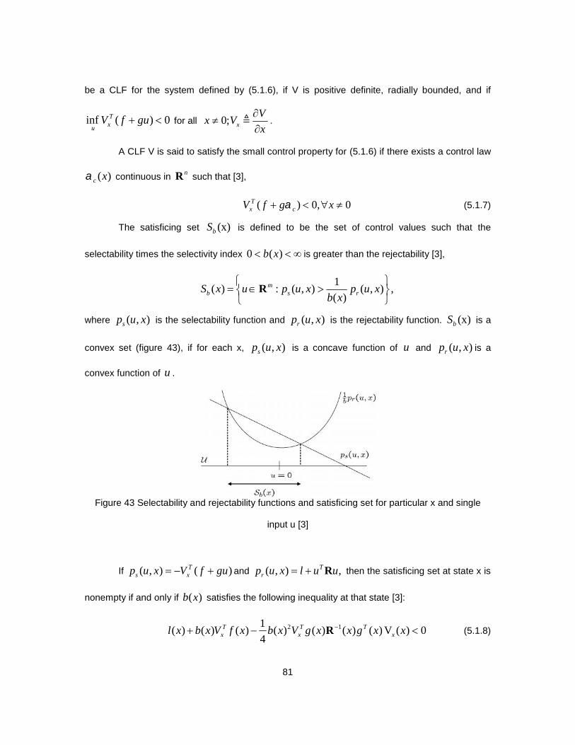
81
be a CLF for the system defined by (5.1.6), if V is positive definite, radially bounded, and if
inf ( ) 0Tx
uV f gu for all 0; x
Vx V
x
.
A CLF V is said to satisfy the small control property for (5.1.6) if there exists a control law
( )c x continuous in nR such that [3],
( ) 0, 0Tx cV f g x (5.1.7)
The satisficing set (x)bS is defined to be the set of control values such that the
selectability times the selectivity index 0 ( )b x is greater than the rejectability [3],
1( ) : ( , ) ( , ) ,
( )m
b s rS x u p u x p u xb x
R
where ( , )sp u x is the selectability function and ( , )rp u x is the rejectability function. (x)bS is a
convex set (figure 43), if for each x, ( , )sp u x is a concave function of u and ( , )rp u x is a
convex function of u .
Figure 43 Selectability and rejectability functions and satisficing set for particular x and single
input u [3]
If ( , ) ( )Ts xp u x V f gu and ( , ) ,T
rp u x l u u R then the satisficing set at state x is
nonempty if and only if ( )b x satisfies the following inequality at that state [3]:
2 11( ) ( ) ( ) ( ) ( ) ( ) ( ) V ( ) 0
4T T T
x x xl x b x V f x b x V g x x g x x R (5.1.8)

82
It shows that the selectivity index ( )b x plays a critical role in the size of ( )bS x . The nonempty
( ) mbS x R is [3],
1 1/2 2 11 1( ) : 1
2 4T T T T
b x x x xS x b g V b V g g V l bV f
R R R (5.1.9)
For the satisficing set to be nonempty at each 0x [3],
2 1
1
1,ifV 0
( )2 2
,
TxT
x
T T T Tx x x x
T Tx x
gV f
b xV f V f lV g g V
otherwiseV g g V
R
R
(5.1.10)
From [3], it can be proved that if V is a CLF for system (5.1.6), b is given by (5.1.10) and
bS is given by (5.1.9), then for each 0x
1. ( ) 0b x ;
2. ( )b b x implies that ( ) ;bS x
3. If : nl R R satisfies the property
( 0 0) 0T Tx xg V andV f l (5.1.11)
then ( )b x is locally Lipschitz on \ 0 .nR The following are defined as in [3],
11
1( , )
2T
xx b b g V R (5.1.12)
1/2 2 12
1( , )
4T T T
x x xx b b V g g V l bV f R R (5.1.13)
Now the union of ( )bS x overall ( )b b x can be taken for all 0x to obtain
1 2( ) ( , ) ( , ) : ( ), 1S x x b x b b b x (5.1.14)
Then, ( )S x is guaranteed to be nonempty for 0x . Thus, the satisficing set is parameterized by
the selection functions : nb R R and : n m R R , where ( ) ( )b x b x and ( ) 1.x

83
5.1.3.2 Satisficing Controls
Curtis and Beard [3] defined satisficing controls to be locally Lipschitz selections from the
satisficing set. It asymptotically stabilize the closed-loop system.
The mapping : n mk R R is called a satisficing control for the system (5.1.6) if [3],
1. (0) 0k ;
2. ( ) ( )k x S x for each \ 0 ;nxR
3. k is locally Lipschitz on \ 0 .nR
The following parameterizes the set of satisficing controls via two locally Lipschitz
selection functions [3]:
If
1. V is a CLF for system (5.1.5);
2. : n m R R is locally Lipschitz on \{0}nR and satisfies ( ) 1;x
3. b : n R R is locally Lipschitz on \{0}nR and satisfies ( ) b(x);b x
then
1 2
0, 0( )
( , ( )) ( , ( )) (x),
xk x
x b x x b x otherwise
(5.1.15)
is a satisficing control for system (5.1.6). Moreover, as V satisfies the small control
property, ( ) ( ) ( )b x x b x in a neighborhood close to the origin; where 1 ( ) ,x N and
( )xR satisfies ( ) ,rI x rI x R , where r and r are positive constants, then k is
continuous at the origin. Then, inverse optimality is also proven. This satisficing approach can be
used for the design and analysis of nonlinear control problems [3].

84
References
1. Satisficing from Wikipedia
2. Michael A. Goodrich, Wynn C. Stirling and Richard L. Frost, “A theory of satisficing
decision and control,” IEEE TRANSACTIONS ON SYSTEMS, MAN, AND CYBERNATICS-PART
A: SYSTEMS AND HUMANS, VOL. 28, NO. 6, NOV. 1998, pp. 763-779.
3. J. W. Curtis, R. W. Beard, “Satisficing: A new approach to constructive nonlinear control”,
IEEE TRANSACTIONS ON AUTOMATIC CONTROL, VOL. 49, NO. 7, JULY 2004, pp. 1090-
1102.
4. Samuel J. Gershman, Jonathan D. Cohen, Yael Niv, “Learning to Selectively Attend”,
Cognitive Science Society, 2006, pp. 1270-1275.

85
5.2 Satisficing Games
Section 5.1 explained about satisficing and its use to control a single agent/system. Now
this section illustrates its use in game theory. It mainly involves the work done by Stirling.
5.2.1 Satisficing in Game Theory
Stirling and Goodrich introduced the concept of satisficing in game theory [1-3]. In their
work, notion of ‘comparative rationality’ is defined for satisficing. Preferences of m-agents are
prescribed by a 2m-dimensional ‘interdependence function and the set of jointly satisficing
decision is derived. This satisficing decisions are robust and functional which can deal with
uncertainty very efficiently. Then the authors analyzed some games using this theory.
Game theory is a theory of decision making in which two or more agents/decision makers
are involved. The game generally consists of players, preferences and choices of players, rules,
probabilities, outcomes and payoffs. Nash equilibria, dominance and Pareto-optimality are the
most highly developed solutions derived by extending the principle of optimality to a multi-agent
domain; individual optimality is not always jointly optimal, so a satisficing solution is found. It is
common to evaluate options by comparing potential gains with potential losses and choosing the
one for which the gain exceeds the losses. This decision is called ‘comparatively rational’. This
comparative rational decision is defined by the authors as a satisficing one. The notion of
epistemic utility theory is used which was explained in the previous section (5.1.2). Expression of
utility theory in the language of probability makes it well equipped to extend from single-agent
games to multi-agent games. Requirement of multi-variate credibility (benefit, gain) and
rejectability (cost, lost) functions is the main difference. These derivation is performed by
interdependence function [3].
Accuracy (benefit) and liability (cost) are assumed to be independent concepts. This
means that it is neither a guaranty nor a necessity to simply consume the resources for
achievement of the goal. When the joint credibility/rejectability function factors into the product of

86
the ‘marginal’ credibility and liability function for a single agent, it called the ‘intra-dependence’ of
accuracy and liability. It generally holds for single agent decision problems; but not for multi-agent
decision problems [3].
Consider a system of m agents 1,..., mX XX . iU denotes the decision or option
space for agent iX , iF denotes the Boolean algebra of option sets available to iX . A satisficing
game is defined as the probability space 1, , P ,CR mU U U U U is the multipartite
option space, 1 mF F is a Boolean algebra of multi-partite option sets, and
: [0,1]CRP is a probability measure over , the smallest Boolean algebra that
contains all products of measurable rectangles of the form V W , with , V W . This is
represented as ( , )CRP V W , interdependence measuring function of two set variables, where V
is a measurable subset of U with respect to which credibility is considered, and W is a
measurable subset of U with respect to which rejectability is considered. It characterizes the joint
credibility/rejectability of all elements of ; that is, for V and W , ( , )CRP V W
expresses the accuracy associated with V and the liability associated with W .
Let 1 mV V V and 1 mW W W be rectangles in U . The interdependence
measure can be rewritten as 1 1 1 1, , , , , W
m mC C R R m mP V V W . Since U is discrete, the
interdependence probability mass function can be defined as [3],
1 1 1 11 1 1 1, , , , , W , , , , ,
m m m mC C R R m m C C R R m mP V V W P v v w w (5.2.1)
where iv and iw are singleton sets in iF , i = 1,..., m. The interdependence function
represents the joint benefit and cost of iX considering the adoption of iv from the perspective of
accuracy (achieving the goal) and, simultaneously, considering the adoption of iw from the
perspective of liability (being exposed to things undesirable), for i = 1,..., m. This function simply

87
encodes the information. The function can be factored into a product of conditional probability
mass functions which makes the specification the conditional behavior easier. Due to modularity
features, it can be used to characterize local or specific responses. For two agents, the
interdependence function may be factored as [3],
1 2 1 2 1 1 2 2 2 2
1 2 1 2 1 2 2 2 2 2
1 2 1 2 |C 1, 1 2 2 2 2
| 1 2 1 2 | 1 2 2 | 2 2 2
, , , w ( | , ) ( , )
| , , w | , w | w w
C C R R C R R C R
C C R R R C R C R R
P v v w P v w v w P v w
P v v w P w v P v P
where 1 2 1 2| 1 2 1 2| , , wC C R RP v v w represents 1X 's conditional credibility given that 2X places its
entire unit of credibility mass on 2v and all of its rejectability mass on 2w , and 1X places all of its
rejectability mass on 1v . Also, 1 2 2| 1 2 2| , wR C RP w v represents 1X 's rejectability of 1w given that
2X places all of its credibility mass on 2v and all of its rejectability mass on 2w . Due to intra-
independence for single agents, 2 2 2| 2 2 2| wC R CP v P v . The probabilities
2CP and2RP
represent 2X 's myopic (isolation from the influence from others) credibility and rejectability,
respectively.
. The satisficing set is obtained via Levi's rule, which requires the multi-variate credibility
and rejectability probability mass functions, CP and RP . These functions can be obtained as
follows [3],
( ) ( , )C CRP P
w U
v v w (5.2.2)
( ) ( , )R CRP P
v U
w v w (5.2.3)
and Levi's rule is extended to the multi-agent case by defining the Multipartite Rule of Epistemic
Utility [3]:
: ( ) ( )b C RS P bP u U u u (5.2.4)
bS is termed the multipartite satisficing set, and elements of bS are multipartite satisficing
options. This is strengthened by restricting attention to the multi-partite strictly satisficing options

88
: ( ) ( )b C RS P bP u U u u (5.2.5)
Now, this can be applied to multi-player games that illustrate epistemic utility-based satisficing.

89
References
1. Matthew Nokleby, Wynn Stirling, “Attitude Adaptation in Satisficing Games”, IEEE
TRANSACTIONS ON SYSTEMS, MAN, AND CYBERNETICS, PART B: CYBERNETICS, VOL.
39, NO. 6, DEC. 2009, pp. 1556-1567.
2. Wynn C. Stirling, “Satisficing Games and Decision Making”, Cambridge University Press
(Book), 2003.
3. Wynn C. Stirling, Michael A. Goodrich, “Satisficing games”, Information Sciences 1999,
pp. 255-280.
4. Surachai Charoensri, H.W. Corley, “The Scalarization and Equivalence of Standard
Optimization Criteria”, COSMOS Technical Report 11-03.

90
Chapter 6
Bounded Rationality
6.1 What is Bounded Rationality?
This section throws light on another concept of human decision making which is called
‘Bounded rationality’. It is based on the limitation of resources and time available for decision
making. This way it is related with satisficing discussed in the previous chapter. The first sub-
section explains the concept of bounded rationality. The following sections relate it to psychology,
economics and management. It includes the work done by Kahneman, Castellaneta, Fogel,
Vreeswijk and Park.
6.1.1 Introduction
Decision-making is viewed in economics and related disciplines as a fully rational
process that finds the optimal choice. But Herbert Simon proposed the idea of ‘bounded
rationality’ in decision making because the optimality of individuals is limited by the availability of
information, limited cognitive skills and the constraint of time. Another point of view is that the
people simplify the available choices and then only apply their rationality. Thus the decision-
maker is one seeking a satisfactory solution rather than the optimal one, a ‘satisficer’. Simon
compares bounded rationality with of a pair of scissors where one blade is the "cognitive
limitations" of actual humans and the other the "structures of the environment". Thus, pre-existing
structures and regularity in the environment can be successfully exploited with the limitations [1].
Some models in the social sciences assume humans as "rational" entities. People are
assumed to be on an average as rational and they are approximated to act according to
their preferences (selective attention, Reyna-2012). This is in contrast to the concept bounded
rationality that finite computational resources hinder the feasibility of making rational choices [1].
Simon suggests that when most people make decisions, they are only partly rational and partly
irrational. He also suggests that boundedly rational agents face constraints in formulating and

91
solving complex problems, and in receiving, storing, retrieving, and transmitting information. He
describes a number of dimensions including limited the types of utility functions, the costs and
possible multi-valued utility function, along which rationality can be made somewhat more realistic
with a rigorous formalization. He also suggests the use of heuristics in decision making instead of
a rigid rule of optimization [1].
Ariel Rubinstein proposed that bounded rationality should be modeled by explicitly
specifying decision-making procedures including deciding the method and time of the decision.
Gerd Gigerenzer opines that decision theorists have not really adhered to Simon's original ideas.
Rather, they have assumed that either decisions are crippled by limitations or people try to cope
with their inability to optimize. Gigerenzer proposes and shows that simple heuristics often lead to
better decisions than optimality [1].
Edward Tsang suggests that computational intelligence can be used to measure degree
of rationality of a decision-maker. This is based on a proposal that decision procedure can be
encoded in algorithms along with heuristics. An agent with higher computational intelligence can
make choice nearer to optimality than one with lower algorithms and heuristics, considering
everything else being equal [1].
6.1.2 Bounded Rationality and Behavioral Psychology:
Kahneman [2] along with others attempted to explore the psychology of intuitive beliefs
and choices and examined their bounded rationality. The research obtained a map of bounded
rationality by distinguishing between the beliefs of people (including optimal one) and the choices
assumed in rational-agent models. This was the start and the main source of their null
hypotheses. They had three research programs: (1) First explored the heuristics used by people
along with the biases to make decisions under uncertainty, including predictions and evaluations
of evidence, (2) The second was related with prospect theory, risky choice model and, (3) The
third one dealt with framing effects and their implications.

92
6.1.2.1 Architecture of Cognition:
Kahneman [2] distinguishes two modes of thinking and deciding, of reasoning and
intuition. Reasoning is related to the cognitive process undertaken while computing the product of
17 by 258. Intuition similar to the gists, essential meaning. Reasoning is a deliberate and effortful
process, but intuitive thoughts come spontaneously with almost no effort of search or
computation. Research has given an indication of intuitive thoughts and actions most of the times.
Figure 44 Cognitive system architecture [2]
Figure 44 shows the widely agreed, different characteristics of reasoning and intuition.
These two types of cognitive processes were proposed (Stanovich and West 2000) to be
neutrally labeled as System 1 and System 2. The scheme shown in Figure 49 summarizes these
characteristics. The operations of System 1 are uncontrollable as they are governed by habit,
influenced by emotions, fast, automatic, effortless, and associative; while the System 2 has
slower, serial, rule-governed, effortful, and deliberately controlled. Though, sometimes System 2
is faster than System 1 (Levine, Ramirez Jr., McClelland, Rebecca Robinson, & Krawczyk, 2014).

93
The most useful characteristic that can be used to classify a mental process into System 1 or
System 2 is the difference in effort. With total capacity being limited, effortful processes interfere
with each other, whereas effortless processes do not while multi-tasking. As an example, a skillful
driver can do driving and talking simultaneously with very less effort. Different tasks require
different amount of attentional demands and different levels of involvement of System 1 and
System 2. For example, the self-monitoring function belongs to System 2. People occupied in a
demanding mental activity would respond to another task by first instantaneous thought. Both,
System 1 and System 2 can deal with stored information (experiences and knowledge). Thus, it
can be hypothesized that a high numeracy person can deal with probabilities with just intuition;
while the person low in numeracy would have to use reasoning [2].
6.1.2.2 Dimension of Accessibility:
Kahneman explains the accessibility dimension in [2]. It is a technical term indicates that
how easily thoughts come to mind. Some thoughts are accessible and others are not.
Figure 45 Different accessibility dimension example [2]
The first ideas that come to mind by looking at the figure 45 are the height of the tower
and the area of the top surface. These two impressions are highly accessible, though calculating
height or area would require a deliberate operation. For the figure 45a, other attributes such as
the area covered by blocks of the dismantled tower is not accessible, though it can be estimated

94
by a deliberate procedure by multiplying the area of a block by the number of blocks. The
situation is reversed with figure 45b. An impression of total area is immediately accessible, but
the height of the tower constructed from is inaccessible. Additionally, some relational properties
like, similarity (height) between figure 45a and figure 45c and dissimilarity (height) between figure
45b and figure 45a (or 45c) are easily accessible [2]. This relates to bounded rationality as the
accessibility of dimension are bounded.

95
References
1. Bounded Rationality from Wikipedia
2. Daniel Kahneman, “Maps of Bounded Rationality: Psychology for Behavioral
Economics”, THE AMERICAN ECONOMIC REVIEW, 2003, pp. 1449-1474.
3. Francesco Castellaneta, “The boundaries of bounded rationality: Experience, superstition
and the weight of activity load in management buyouts”, Strategic Management Journal, 2014,
pp. 1-41.
4. David B. Fogel, Kumar Chellapilla, and Peter J. Angeline, “Inductive Reasoning and
Bounded Rationality Reconsidered”, TRANSACTIONS ON EVOLUTIONLARY COMPUTATIONS,
VOL. 3, NO. 2, JULY 1999, pp. 142-146.
5. Jaap Vreeswijk, Jing Bie, Eric van Berkum, Bart van Arem, “Effective traffic management
based on bounded rationality and indifference bands”, IET Intelligent Transport Systems, Vol. 7,
Issue 3, 2013, pp. 265-274.
6. Hyunggon Park, Mihaela van der Schaar, “On the Impact of Bounded Rationality in Peer-
to-Peer Networks”, IEEE SIGNAL PROCESSING LETTERS, VOL. 16, NO. 8, AUGUST 2009, pp.
675-678.
7. Daniel S. Levine, Patrick A. Ramirez Jr., M. Michelle McClelland, Rebecca Robinson and
Daniel C. Krawczyk, “Ratio Bias Revisited: Behavioral and Brain Imaging Studies of Ratio
Comparison Tasks”, Thinking and Reasoning, 2014 (In review).
8. Valerie F. Reyna, “A New Intuitionism: Meaning, Memory and Development in Fuzzy
Trace Theory”, Judgment and Decision Making, Vol. 7, No. 3, 2012, pp. 332-359.

96
6.2 Metacognition
6.2.1 Introduction
Metacognition is "cognition about cognition", or "knowing about knowing”. It involves
knowledge about timing and methodology to use a strategy for problem solving. An important
form of metacognition is ‘metamemory’, which is described as knowing about memory and
mnemonic strategies [1].
J. H. Flavell first used the word "metacognition". In his words: Metacognition refers to
one’s knowledge concerning one's own cognitive processes or anything related to them, e.g., the
learning-relevant properties of information or data. For example, I am engaging in metacognition
if I notice that I am having more trouble learning A than B; if it strikes me that I should double
check C before accepting it as fact.
—J. H. Flavell (1976, p. 232).
A. Demetriou, used the term hypercognition to referring to self-monitoring, self-
representation, and self-regulation processes which participate in general intelligence, and
processing efficiency and reasoning. Metacognitive skills include study skills, memory
capabilities, and the ability to monitor learning. These capacities are used to regulate one's own
cognition, maximization of thinking potential, and learning and evaluation of rules [1].
In cognitive neuroscience, it has been found that the prefrontal cortex monitors and
controls metacognition by receiving sensory signals from other cortical regions and through
feedback loops, respectively. In the domain of artificial intelligence and modeling, metacognition
is of interest of emergent systemics. It is used to denote self-awareness of mortality [1].
6.2.2 Components of Metacognition
Metacognition is generally classified into three components [1]:
1. Metacognitive knowledge is awareness about own self others as cognitive
processors.

97
2. Metacognitive regulation is the regulation of cognition and learning experiences
through a set of activities.
3. Metacognitive experiences are those experiences that related with the current,
on-going cognitive endeavor.
Metacognition involves active control over the process of thinking that is used in learning.
Planning of the approach to a learning task, monitoring comprehension, and evaluation of the
progress towards the completion of a task are some of the metacognitive skills [1].
6.2.2.1 Metacognitive Knowledge
Metacognition includes at least three types of metacognitive awareness [1]:
1. Declarative Knowledge: The knowledge about oneself as a learner and factors
affecting performance, "world knowledge".
2. Procedural Knowledge: The knowledge about executing things. It is displayed as
heuristics and strategies. A high degree of procedural knowledge can allow
individuals to perform tasks more automatically by more efficient access to a
large variety of strategies.
3. Conditional knowledge: understanding of the right moment and reason to use
declarative and procedural knowledge. It facilitates students to allocate their
resources using more effective strategies.
6.2.2.2 Metacognitive Regulation
Similar to metacognitive knowledge, metacognitive regulation or "regulation of cognition"
contains three important skills [1]:
1. Planning: refers to the appropriate selection of strategies and the correct
allocation of resources that affect task performance.
2. Monitoring: refers to one's awareness of comprehension and task performance

98
3. Evaluating: refers to appraising the final product of a task and the efficiency at
which the task was performed. This can include re-evaluating strategies that
were used.
Similarly, sustaining motivation and effort till the task end along with the awareness of
both internal and external distracting stimuli involve metacognitive functions. Students high in
metacognition can perform more efficiently with fewer strategies without any prior knowledge [1].
6.2.2.3 Metacognitive Experience
Metacognitive experience is creates the identity of one’s self and it is linked to motivation.
Identity is important as it provides a support for meaning making and for action. Importance of
identity is determined with meta-cognitive experience by comparing its worth to other important
identities and whether and then its pursuance or abundance is decided. Metacognitive difficulty is
considered as a link to abandoning identity. Theories like the theory of incremental ability put
difficulty as a way to pursue an identity in which when effort is important, more effort required is
termed as difficulty; while the entity theory of ability describes the opposite that when effort is not
of importance, suspension of effort is considered difficulty due to the lack of that ability.
.

99
References
1. Metacognition from Wikipedia

100
Bibliography
1. Abdesselam Bouzerdoum, “Classification and Function Approximation using Feed-
Forward Shunting Inhibitory Artificial Neural Networks”, IJCNN, 2000, pp. 613-618.
2. Bobby Ojose, “Applying Piaget’s Theory of Cognitive Development to Mathematics
Instruction”, The Mathematics Educator, Vol. 18, No. 1, 2008, pp. 26-30.
3. Brenda R. Jansen, Anna C. Duijvenvoorde, Hilde M. Huizenga, “Development of Decision
Making: Sequential versus Integrative Rules”, Journal of Experimental Child Psychology 111,
2012, pp. 87-100.
4. Christian Balkenius, Stefan Winberg, “Cognitive Modeling with Context Sensitive
Reinforcement Learning”, Proceedings of AILS 04, 2004, pp. 10-19.
5. Daniel Kahneman, “Maps of Bounded Rationality: Psychology for Behavioral
Economics”, The American Economic Review, 2003, pp. 1449-1474.
6. Daniel S. Levine, “Emotion and Decision Making: Short-term Reactions versus Long-term
Evaluations”, International Joint Conference on Neural Networks, 2006, pp. 195-202.
7. Daniel S. Levine,” Modeling the Evolution of Decision Rules in the Human Brain”,
International Joint Conference on Neural Networks, 2006, pp. 625-631.
8. Daniel S. Levine, “Neural Dynamics of Affect, Gist, Probability, and Choice”, Cognitive
System Research, Science-Direct, 2012, pp. 57-72.
9. Daniel S. Levine, “Seek Simplicity and Distrust it: Knowledge Maximization versus Effort
Minimization”, KIMAS talk, 2007.
10. Daniel S. Levine, Britain Mills, Steven Estrada, “Modeling Emotional Influences on
Human Decision Making under Risk”, IJCNN Special Session, Vol. 3, 2005, pp. 1657-1662.
11. Daniel S. Levine, Leonid I. Perlovsky, “A Network Model of Rational versus Irrational
Choices on a Probability Maximization Task”, IJCNN, 2008, pp 2820-2824.
12. Daniel S. Levine, Patrick Ramirez, “An Attentional Theory of Emotional Influences on
Risky Decisions”, Progress in Brain Research, Vol. 202, Elsevier (Book), 2013.
101
13. Daniel S. Levine, Patrick A. Ramirez Jr., M. Michelle McClelland, Rebecca Robinson and
Daniel C. Krawczyk, “Ratio Bias Revisited: Behavioral and Brain Imaging Studies of Ratio
Comparison Tasks”, Thinking and Reasoning, 2014 (In review).
14. David B. Fogel, Kumar Chellapilla, and Peter J. Angeline, “Inductive Reasoning and
Bounded Rationality Reconsidered”, Transactions On Evolutionary Computations, Vol. 3, No. 2,
JULY 1999, pp. 142-146.
15. Edward T. Cokely, Colleen M. Kelley, “Cognitive Abilities and Superior Decision Making
under Risk: A Protocol Analysis and Process Model Evaluation”, Judgment and Decision Making,
Vol. 4, No. 1, February 2009, pp. 20–33.
16. Francesco Castellaneta, “The Boundaries of Bounded Rationality: Experience,
Superstition and the Weight of Activity Load in Management Buyouts”, Strategic Management
Journal, 2014, pp. 1-41.
17. Ganesh Arulampalam, Abdesselam Bouzerdoum, “A Generalized Feedforward Neural
Network Architecture for Classification and Regression”, Neural Networks 16, 2003, pp. 561–568.
18. http://www.wikipedia.org/
19. Hyunggon Park, Mihaela van der Schaar, “On the Impact of Bounded Rationality in Peer-
to-Peer Networks”, IEEE Signal Processing Letters, Vol. 16, No. 8, August 2009, pp. 675-678.
20. Jaap Vreeswijk, Jing Bie, Eric van Berkum, Bart van Arem, “Effective Traffic Management
based on Bounded Rationality and Indifference Bands”, IET Intelligent Transport Systems, Vol. 7,
Iss. 3, 2013, pp. 265-274.
21. J. W. Curtis, Randal W. Beard, “Satisficing: A New Approach to Constructive Nonlinear
Control”, IEEE Transactions on Automatic Control, Vol. 49, No. 7, July 2004, pp. 1090-1102.
22. Joshua Brown, Daniel Bullock, Stephen Grossberg, “How the Basal Ganglia use Parallel
Excitatory and Inhibitory Learning Pathways to Selectively Respond to Unexpected Rewarding
Cues”, The Journal of Neuroscience, 1999, pp. 10502–10511.
23. Kenji Doya, “What are the Computations of the Cerebellum, the Basal Ganglia and the
Cerebral Cortex?”, Neural Networks 12, 1999, pp. 961-974.

102
24. Kenji Doya, Hidenori Kimura, Aiko Miyamura, “Motor Control: Neural Models and System
Theory”, International Journal of Applied Mathematics and Computer Science, Vol. 11, 2001, pp.
101-128.
25. Kenji Doya, Hidenori Kimura, Mitsuo Kawato, “Neural Mechanisms of Learning and
Control,” IEEE Control System Magazine, Vol. 21, 2001, pp. 42-54.
26. Kenji Doya, Kazuyuki Samejima, Ken-ichi Katagiri, Mitsuo Kawato, “Multiple Model-
Based Reinforcement Learning”, Neural Computation, 2002, pp. 1347-1369.
27. Kumpati Narendra, Jeyendran Balakrishnan, “Adaptive Control using Multiple Models”,
IEEE Transactions on Automatic Control, Vol. 42, No. 2, 1997, pp. 171-187.
28. Mathieu Bertin, Nicolas Schweighofer, Kenji Doya, “Multiple Model-based Reinforcement
Learning Explains Neuronal Dopamine Activity”, Neural Networks 20, 2007, pp. 668–675.
29. Matthew Nokleby, Wynn Stirling, “Attitude Adaptation in Satisficing Games”, IEEE
Transactions on Automatic Control, Man, and Cybernetics, Part B: Cybernetics, Vol. 39, No. 6,
December 2009, pp. 1556-1567.
30. Mehdi Khamassi, Stéphane Lallée, Pierre Enel, Emmanuel Procyk, Peter F. Dominey,
“Robot Cognitive Control with a Neuro-physiologically Inspired Reinforcement Learning Model”,
Forntiers in Neurorobotics, Volume 5, Article 1, 2011, pp. 1-14.
31. Michael A. Goodrich, Wynn C. Stirling and Richard L. Frost, “A Theory of Satisficing
Decision and Control,” IEEE Transactions on Automatic Control, Man, and Cybernetics-Part A:
Systems and Humans, Vol. 28, No. 6, November 1998, pp. 763-779.
32. Norikazu Sugimoto, Jun Morimoto, Sang-Ho Hyon, Mitsuo Kawato, “The eMOSAIC
Model for Humanoid Robot Control”, Neural Networks, 2012, pp. 8-19.
33. Okihide Hikosaka, Hiroyuki Nakahara, Miya K. Rand, Katsuyuki Sakai, Xiaofeng Lu, Kae
Nakamura, Shigehiro Miyachi, Kenji Doya, “Parallel Neural Networks for Learning Sequential
Procedures”, TINS Vol. 22, No. 10, 1999, pp. 464-471.

103
34. Paul J. Werbos, “Handbook of Intelligent Control: Neural, Fuzzy and Adaptive
Approaches”, Van Nostrand Reinhold, 1992, pp. 493-525.
35. Paul J. Werbos, “Intelligence in the Brain: A Theory of How it Works and How to Build it”,
Neural Networks 22, 2009, pp. 200-212.
36. Paul J. Werbos, “Neural Networks and the Human Mind: New Mathematics Fits
Humanistic Insight”, IEEE International Conference on Systems, Man, and Cybernetics, vol. 1,
1992, pp. 78-83.
37. Paul J. Werbos, “Using ADP to Understand and Replicate Brain Intelligence: the Next
Level Design”, IEEE International Symposium on Approximate Dynamic Programming and
Reinforcement Learning, 2007, pp. 209-216.
38. Paul Werbos, “What is Mind? What is Consciousness? How Can We Build and
Understand Intelligent Systems?”, Werbos’ website.
39. Petru E. Stingu, Frank L. Lewis, “Neuro Fuzzy Control of Autonomous Robotics”,
Springer (Book), 2009.
40. R. Nieuwenhuys, J. Voogd, C. van Huijzen, “The Human Central Nervous System”, Forth
Edition, Springer (Book), 2008.
41. Ranuifo Romo, Eugenio Scarnati, Wolfram Schultz, “Role of Primate Basal Ganglia and
Frontal Cortex in the Internal Generation of Movements-II. Movement Related Activity in the
Anterior Striatum”, Experimental Brain Research 91, 1992, pp. 385-395.
42. Ranuifo Romo, Wolfram Schultz, “Role of Primate Basal Ganglia and Frontal Cortex in
the Internal Generation of Movements-III. Neuronal Activity in the Anterior Striatum”,
Experimental Brain Research 91, 1992, pp. 396-407.
43. Samuel J. Gershman, Jonathan D. Cohen, Yael Niv, “Learning to Selectively Attend”,
Cognitive Science Society, 2006, pp. 1270-1275.
44. Surachai Charoensri, H.W. Corley, “The Scalarization and Equivalence of Standard
Optimization Criteria”, COSMOS Technical Report 11-03.

104
45. Tetsuya Minatohara, Tetsuo Furukawa, “The Self-Organizing Adaptive Controller”,
International Journal of Innovative Computing, Information and Control, Vol 7, number 4, April
2011, pp. 1933-1947.
46. Valerie F. Reyna, “A New Intuitionism: Meaning, Memory and Development in Fuzzy
Trace Theory”, Judgment and Decision Making, Vol. 7, No. 3, 2012, pp. 332-359
47. Wolfram Schultz, Ranuifo Romo, “Role of Primate Basal Ganglia and Frontal Cortex in
the Internal Generation of Movements-I. Preparatory Activity in the Anterior Striatum”,
Experimental Brain Research 91, 1992, pp. 363-384.
48. Wolfram Schultz, Leon Tremblay, Jeffrey R. Hollerman, “Reward Prediction in Primate
Basal Ganglia and Frontal Cortex”, Neuropharmacology 37, 1998, pp. 421-429.
49. Wolfram Schultz, Leon Tremblay, Jeffrey R. Hollerman, “Reward Processing in Primate
Orbitofrontal Cortex and Basal Ganglia”, Cerebral Cortex, 2007, pp. 272-283.
50. Wynn C. Stirling, “Satisficing Games and Decision Making”, Cambridge University Press
(Book), 2003.
51. Wynn C. Stirling, Michael A. Goodrich, “Satisficing games”, Information Sciences 1999,
pp. 255-280.

105
Biographical Information
Patanjalikumar Shashankkumar Joshi graduated with a degree of Master of Science in
Electrical Engineering from University of Texas at Arlington in December, 2014. He has worked at
University of Texas at Arlington Research Institute under the supervision of Dr. Frank L. Lewis
from January, 2013 to December, 2014. He earned his Bachelor of Engineering degree in
Electronics and Communications Engineering in July, 2011 from Sardar Patel University, India.
His area of interests are control systems, automation and robotics. He is also interested in
embedded microcontroller/microprocessor systems.