a level set framework for capturing multi-valued solutions of

DOI: 10.1007/s10915-005-9016-1Journal of Scientific Computing, Vol. 29, No. 3, December 2006 (© 2005)

A Level Set Framework for Capturing Multi-ValuedSolutions of Nonlinear First-Order Equations

Hailiang Liu,1 Li-Tien Cheng,2 and Stanley Osher3

Received December 13, 2004; accepted (in revised form) April 9, 2005; Published online December 7, 2005

We introduce a level set method for the computation of multi-valued solutionsof a general class of nonlinear first-order equations in arbitrary space dimen-sions. The idea is to realize the solution as well as its gradient as the com-mon zero level set of several level set functions in the jet space. A very genericlevel set equation for the underlying PDEs is thus derived. Specific forms ofthe level set equation for both first-order transport equations and first-orderHamilton-Jacobi equations are presented. Using a local level set approach, themulti-valued solutions can be realized numerically as the projection of single-valued solutions of a linear equation in the augmented phase space. The levelset approach we use automatically handles these solutions as they appear.

KEY WORDS: level set method; multi-valued solutions; nonlinear first-orderequations.

AMS subject classification: Primary 35F25; Secondary 65M25

1. INTRODUCTION

Numerical simulations of high-frequency wave propagation are importantin many applications. When the wave field is highly oscillatory in thehigh-frequency regime, direct numerical simulation of the wave field canbe prohibitively costly. Examples include the semiclassical limit for theSchrodinger equation and geometric optics for the wave equation. A nat-ural way to remedy this problem is to use some approximate model which

1 Mathematics Department, Iowa State University, Ames, IA 50011, USA. E-mail: [email protected]

2 Mathematics Department, UC San Diego, La Jolla, CA 92093-0112, USA. E-mail:[email protected]

3 Level Set Systems Inc., 1058 Embury Street, Pacific Palisades, CA 90272-2501, USA.E-mail: [email protected]

353

0885-7474/06/1200-0353/0 © 2005 Springer Science+Business Media, Inc.

354 Liu, Cheng, and Osher

can resolve the small-scale in the wave field. The classical approach is theWentzel–Kramers–Brillonin (WKB) method or geometric optics, which areasymptotic approximations obtained when the small scale becomes finer.Instead of the oscillating wave field, the unknowns in the WKB system arethe phase and the amplitude, neither of which depends on the small scale,and typically vary on a much coarser scale than the wave field. Hence theyare usually easier to compute numerically.

An obvious drawback of this method is that linear equations arereplaced by nonlinear ones, and thereby the superposition principle is lost.In the WKB system the phase is often described by Hamilton-Jacobi (HJ)equations; unfortunately, the classical viscosity solutions [10] are not ade-quate in describing the superposition nature of waves in phase space. Anatural way to avoid such difficulties is to seek multi-valued solutions cor-responding to crossing waves. In the last decade, various techniques havebeen introduced for multi-phase computations found in several applica-tions. Consult [14] for a recent survey on computational high-frequencywave propagation. In [9] we introduced a level set framework to computethe multi-valued solutions to HJ equations, with application to the semi-classical limit of the linear Schrodinger equation.

The goal of our work here is to extend the ideas developed in [9]and [22] for the computation of multi-valued solutions of a very generalclass of nonlinear first-order equations including ∂tS +H(x,S,∇xS)= 0,to which the previous studies conducted in [9, 22] do not apply. Recentlymathematical theory of multi-valued solutions has further been developedin [23], where a notion of geometrical solutions is adopted based on levelset formulations introduced in this paper. The well-posedness of the geo-metrical solutions of HJ equations is established and the relation withentropy and viscosity solutions is clarified.

We begin by sketching the ideas explored in [9], where we focused onthe computation of multi-valued solutions of the HJ equation

∂tS+H(x,∇xS)=0, x ∈ IRn, (1.1)

which appears as the phase equation in the semiclassical limit of the lin-ear Schrodinger equation. The level set functions φ(t, x,p), defined in thephase space (x,p) ∈ IR2n, with p = ∇xS, each satisfies a linear Liouvilleequation,

∂tφ+∇pH ·∇xφ−∇xH ·∇pφ=0 (1.2)

and the multi-valued phase gradient is captured as the intersection of thezero level sets of n+ 1 level set functions (see also [22]). However in thesemiclassical regime of the Schrodinger equation, there is also a need to

Multi-Valued Solutions of Nonlinear First-Order Equations 355

resolve the multi-valued phase value S(t, x) in the whole domain. In thecontext of geometric optics, the phase remains constant along the ray [27](as it does for any Hamiltonian which is homogeneous of degree one in∇S); the wavefront is therefore defined as the level curve of the phase andthe phase solution is completely determined by computing the wavefrontlocation. However in the Schrodinger setting the phase S does change itsshape along the ray in (x,p) space. In [9] we defined the wavefront to bethe n− 1 dimensional surface in (x,p) space, driven by the Hamiltoniandynamics (1.2), and starting with a level surface of the initial phase S0.For the computation of such a defined wavefront, we solve n+ 1 decou-pled level set equations (1.2), n of these functions can be initialized as thecomponents of p−∇xS0, and the remaining one can be initialized as thelevel set of the initial phase, e.g., S0(x)−C.

As pointed out in [9], solving the Liouville equation (1.2) alone is notenough to compute the multi-valued phase S(t, x), even on the wavefrontdescribed above. Note that in the phase space (x,p), the correspondingphase function S(t, x,p) satisfies a forced hyperbolic transport equation

∂t S+∇pH ·∇xS−∇xH ·∇pS=p ·∇pH −H. (1.3)

The strategy in [9] was to look at the graph of the phase functionz= S(t, x,p) in the whole domain, or equivalently to evolve a level setfunction φ=φ(t, x,p, z) in the extended phase space (x,p, z)∈ IR2n+1

∂tφ+∇pH ·∇xφ−∇xH ·∇pφ+ (p ·∇pH −H)∂zφ=0. (1.4)

In this way, wavefronts with possible multi-phases are tracked and thephase value is numerically resolved via the intersection of n+1 zero levelsets in the extended space (x, z,p) ∈ IR2n+1 (see e.g. [6, 9]). In particu-lar, the augmented phase space enables us to track the phase S in theentire domain and then project onto the wavefront surface when desired.Note that the Hamiltonian H in (1.1) does not explicitly depend on S, andtherefore Eq. (1.3) is linear in S. Thus, the singularities of S are already‘unfolded’ in the phase space (x,p)∈ IR2n. For this reason, in [9] we choseto either solve the forced Liouville PDE (1.3) in the whole domain orevolve the whole phase as a zero level set in (x, z,p)∈ IR2n+1, whicheverwas more convenient. We note that the ‘phase space’ idea used in [9] isnot new and has already been extensively explored in various contexts(see, e.g., [7, 15, 26, 33]). However, the level set equation in the jet space(x,p, z) was formulated for the first time in [9] for HJ equation (1.1). Ouraim in this work is to generalize the method in [9] to any first-order PDEsand present some new numerical examples beyond those given in [9].


To put our study in the proper perspective, we recall that there hasbeen a considerable amount of literature available on the computation ofmulti-valued solutions, ranging from geometric optics [1, 11–13, 27] to thesemiclassical regime of Schrodinger equations [9, 17, 21]. In the literature,Lagrangian methods (called ray tracing) and Eulerian methods are thetwo main approaches used to compute multi-valued solutions. An obvi-ous drawback of the former lies in numerically obtaining adequate spatialresolution of the wavefront in regions with diverging rays. This problemis avoided in Eulerian methods through the use of uniform fixed grids intheir computations (see, e.g., [2, 3]). With Eulerian methods, however, diffi-culties arise in handling the multi-valued solutions that appear beyond sin-gularity formation.

A widely acceptable approach for physical space-based Eulerian meth-ods is the use of a kinetic formulation in the phase space, in terms ofa density function that satisfies Liouville’s equation, where the techniqueused to capture multi-valued solutions is based on a closure assumptionof a system of equations for the moments of the density (see [4, 5, 12,16, 17, 21]). In geometric optics and the topic of wavefront construction,geometry-based methods in phase space such as the segment projectionmethod [13], and the level set method [8, 27, 30] have been recently intro-duced. For the computation of multi-valued solutions to the semiclassicallimit of the Schrodinger equation, a new level set method for HJ equa-tions was introduced in [9], to realize the phase S on the whole domainwith the level set evolution in an extended space (x, z,p). Furthermore,wavefronts are constructed via the linear Liouville equation in the (x,p)space. As remarked earlier our key idea is to build both the ‘graph’ andthe ‘gradient’ into the zero level set, allowing for computation of multi-valued solutions in the whole domain of physical interest.

Related to our work in [9], on the computation of multi-valued solu-tions of HJ equation (1.1), is the recent work of [22]. In this paper, theauthors used the level set formulation given in [7] to obtain the sameresult as in this paper for the case of a scalar quasilinear hyperbolic equa-tion. For HJ equations of the type (1.1), where the Hamiltonian doesnot depend on the solution but only on its gradient, the authors in [22]derived the same level set Liouville equations for the gradient of the phasethrough an independent approach involving techniques found in [7] and[33]. They presented numerical results in one and two-dimensions thatrealized the phase gradient for the HJ equation, plotted using the visuali-zation package devised in [24].

In computing the level set equation in phase space, since the area ofinterest is close to the zero level set, it is possible to use fast local level settechniques in the same manner as in, e.g., [8, 9, 27, 30], which will reduce


the computational cost and (recently) also reduce the storage requirements[25].

This paper is organized as follows. In Sec. 2 we list some nonlinearHJ equations which arise in the high-frequency asymptotic approximation.Section 3 is devoted to a derivation of the generic level set equation forfully nonlinear first-order equations of the form G(ξ,u,∇ξ u)= 0. Specificforms of the level set equations for hyperbolic transport equations and HJequations are presented. Also in this section the computation of multi-val-ued solutions for several equations are discussed and the required num-ber of level set functions for realizing the solution as well as the choice ofcorresponding initial data are specified. Finally in Sec. 4 we describe thenumerical strategy used and present some numerical results.

2. THE WKB METHOD AND HAMILTON-JACOBI EQUATIONS

Before introducing our general level set framework for the compu-tation of multi-valued solutions of first-order PDEs, we pause to con-sider some applications in high-frequency wave propagations for whichwe have special HJ equations for the phase function of the wave field.In these cases, the multi-valuedness will reflect the interference of waves.We illustrate as well how nonlinear HJ equations are obtained via theWKB method. Typical applications include the semiclassical limit forSchrodinger equations and geometric optics for the wave equation. Thecommon feature among these problems is the involvement of a smalldimensionless parameter ε serving as the microscopic–macroscopic ratio.We look at the O(ε)-wave length solutions, which can be tracked in onewave packet with a spatial spreading of the order of 1/ε if the initial wavefield is highly oscillating and takes the form

ψ(x,0)=A0(x) exp(iS0(x)/ε). (2.1)

The usual way to tackle this problem is to use the WKB Ansatz, whichconsists of representing the wave field function ψε in the form

ψ(t, x)=Aε(t, x) exp(iS(t, x)/ε). (2.2)

With this decomposition, the most singular part of the wave field ischaracterized by two quantities: the phase function S, which satisfies thenonlinear HJ equation, and the amplitude function A, which satisfies atransport equation.

The derivation of the WKB system in the linear case is classical (see,e.g., Whitham’s book [34]). For linear wave equations subject to highlyoscillatory initial data, insertion of (2.2) into the underlying equations


leads to corresponding relations between the wave’s phase S and its ampli-tude. Splitting the relation into real and imaginary parts and taking thelowest-order (in terms of ε) terms, one often obtains weakly coupledWKB systems of the form

∂tS+H(x,∇xS)=0,

∂tρ+∇x · (ρ∇pH(x,∇xS))=0,

where ρ is related to the amplitude A. We list here two examples, see [32]for more WKB-systems derived from generalized dispersive equations.

(1) Linear Schrodinger equation:

iε∂tψε =−ε

2

2∆ψε +V (x)ψε, x ∈ IRd (2.3)

where V is the corresponding potential, and ε the scaled Planckconstant. In this case H(x,p)= |p|2

2 +V (x) and ρ=A2.(2) The wave equation in an inhomogeneous medium with a variable

local speed c(x) of wave propagation in the medium:

∂2t ψ

ε = c2(x)∆ψε, x ∈ IRd (2.4)

for which we have H(x,p)= c(x)|p| and ρ=A2/c(x).

We note that for the wave equation (2.4), if we look for a planar wavesolution ψ = u(x) exp(it/ε), we are led to a steady state function solvingthe scalar Helmholtz equation

−(∆+k2)u=0, k := (εc(x))−1. (2.5)

Searching for solutions oscillating with frequency 1/ε, we could use theansatz u(x)=A(x) exp(iS(x)/ε), leading to a weakly coupled system,

c(x)|∇xS|=1, ∇x · (A2∇xS)=0. (2.6)

In the paraxial application, one spatial variable is regarded as theevolution direction and the above steady eikonal equation may be writtenas

∂x2S−√c−2 − (∂x1S)

2 =0

or a variant of this (see e.g. [18]). This is again a ‘time-dependent’ HJequation. From the above weakly coupled systems we see that the multi-valued phase S can be computed from the nonlinear HJ equations, inde-pendent of amplitude, and the amplitude is forced to become multi-valuedat points where the phase is multi-valued.


3. LEVEL SET EVOLUTION

Consider a general first-order nonlinear equation

G(ξ,u,∇ξ u)=0, (3.1)

where u∈ IR1 is a scalar unknown and ξ ∈ IRm is the independent variable.Furthermore, G=G(ξ, z, q), (ξ, z, q)∈ IR2m+1 is a given function satisfyingthe nondegeneracy assumption

|∇qG(ξ, z, q)|2 �=0,

which ensures that (3.1) is, in fact, a first-order equation.In order to visualize the solution profile (single-valued or multi-valued),

following [9], we introduce a generic level set function φ(ξ, z, q) in anextended space (ξ, z, q)∈ IR2m+1 so that the solution z=u(ξ), and also itsgradient ∇ξ u, stay on the zero level set

φ(ξ, z, q)=0, z=u(ξ), q=∇ξ u(ξ).Since Eq. (3.1) is a first-order equation, its characteristics exist at leastlocally. Let such characteristics be parameterized as (ξ, z, q)= (ξ, z, q)(τ ).The level set function should be independent of the parameter τ . There-fore,

d

dτφ(ξ(τ ), z(τ ), q(τ ))≡0,

which gives the level set equation

�A ·∇{ξ,z,q}φ=0,

where �A := (dξdτ, dzdτ,dqdτ) denotes the direction field of the characteristics.

According to the classical theory of characteristics for general differen-tial equations of the first order, see [7, pp. 142–144], the vector field isobtained as

A1 =∇qG, A2 =q ·∇qG, A3 =−∇ξG−q · ∂zG.Thus our level set equation is

∇qG ·∇ξφ+q ·∇qG∂zφ− (∇ξG+q∂zG) ·∇qφ=0, (3.2)

which as a linear equation serves to ‘unfold’ multi-valued quantities wher-ever they occur in the physical space. The level set equation in such gener-ality can be used to capture wavefronts, and to recover the solution valueu and the gradient of the solution when desired.


Based on the general level set equation (3.2), we can write down thecorresponding form of the level set equation once the target PDE is given.To implement the level set method for a given problem we still need tofurther check (i) whether reducing to a lower dimension is possible (toreduce computational cost); (ii) how many level set functions are needed;and (iii) how the initial data is chosen. Here are some guiding principles:

• When implementing the level set method, reducing to a lowerdimension is preferred for lowering the computational cost. In gen-eral such reduction is indeed possible if the variables in the lowerdimension give us the quantities we want to compute and thesevariables evolve along the characteristic field independent of othervariables in the full space (ξ, z, q).

• If the reduced space dimension is m and the object of interest is kdimensional, then use m−k level set functions;

• The initial data should be chosen in such a way that the intersec-tion of zero level sets of these chosen initial data uniquely embedsthe given initial data in the original PDE problem.

The level set method has proven to be a powerful tool for capturing thedynamic evolution of surfaces (see [28, 29]). We now demonstrate the levelset method by looking at hyperbolic transport equations and HJ equa-tions, which are two prototypical examples of first-order PDEs. We willstudy how many level set functions are needed to determine the desiredquantities, and how to choose initial data to generate these level set func-tions.

3.1. Hyperbolic Transport Equations

Consider the first-order time-dependent transport equation:

∂tu+F(u, x, t) ·∇xu=B(u, x, t), x ∈ IRn, u∈ IR1 (3.3)

subject to smooth initial data u(0, x)=u0(x).Take ξ= (t, x) and q= (p0, p) with p0 =∂tu, p :=∇xu, and Eq. (3.3)

can be rewritten as G=0 where

G :=p0 +F(z, x, t) ·p−B(z, x, t), z=u.

A simple calculation gives

∇qG ·∇ξφ= ∂tφ+F(z, x, t) ·∇xφ


and

q ·∇qGφz= (1,F ) · (p0, p)=p0 +F ·p=B(z, x, t)φz,where we have used the fact G=p0 +F ·p−B=0. The level set equation(3.2) in this setting reduces to

∂tφ+F ·∇xφ+B∂zφ+A3 ·∇qφ=0.

Note that the transport speeds in the x and z-directions do not explicitlydepend on (p0, p). Therefore, the level set function will not depend on q=(p0, p) if it does not do so initially. Thus, the effective level set equationin the phase space (t, x, z) reads as

∂tφ+F ·∇xφ+B∂zφ=0. (3.4)

The solution u to (3.3) with initial data u(0, x)=u0(x) can be determinedas the zero level set,

φ(t, x, z)=0, z=u(x, t).In this case, we only need one level set function φ. The initial data cansimply be chosen as

φ(0, x, z)= z−u0(x)

or alternatively the signed distance to the surface z=u0(x) in the case ofnonsmooth data. Here the zero level set φ(t, x, u)= 0 can be regarded asa complete integral to (3.4), which implicitly determines u (see [7, p. 140]).

3.2. Generalized Hamilton-Jacobi Equations

Consider a generalized HJ equation

∂tS+H(x,S,∇xS)=0 (3.5)

subject to the initial data

S(x,0)=S0(x), x ∈ IRn. (3.6)

Note, in previous literature, e.g. [10], this equation was simply referred toas HJ equation. Here, we call it generalized HJ equation to distinguish itfrom the case where the Hamiltonian does not depend on S explicitly. Theinclusion of S fundamentally changes the behavior of the solution. Thus,the previous studies conducted in [9] do not apply in this situation.


Taking ξ = (t, x) and q = (p0, p) with p0 = ∂tS, p= ∇xS, Eq. (3.5)can be rewritten as G=0, where

G :=p0 +H(x, z,p), z=S.

A straightforward calculation gives

∂qG ·∇ξφ = ∂tφ+∇pH ·∇xφ,q ·∇qG∂zφ = (p ·∇pH −H)∂zφ

and

∇ξG+q · ∂zG= (0,∇xH)+ (p0, p)Hz= (−HHz,∇xH +pHz),

where we have used p0 = −H(x, z,p). The level set equation in the fullphase space (x, z,p,p0) thus becomes

∂tφ+∇pH ·∇xφ+ (p ·∇pH −H)∂zφ− (∇xH +pHz)∇pφ+HHz∂p0φ=0.

The effective level set equation for (3.5), when capturing p0 =∂tS is not agoal, yields

∂tφ+∇pH ·∇xφ+ (p ·∇pH −H)∂zφ− (∇xH +pHz)∇pφ=0, (3.7)

where φ := φ(t, x, z,p) is well defined in the space (x, z,p) ∈ IR2n+1 forfixed t . The solution S is evolved as the zero level set of φ=φ(t, x, z,p)with z=S, p=∇xS,

Since (p, z)∈ IRn+1, we need (n+1) level set functions φi(t, x, z,p)(i=1, . . . , n+1) in this case. Their common zero level set captures the desiredsolution z=S in the jet space (x,p, z). As a by-product, the multi-valuedp=∇xS will also be determined in this procedure.

For these level set functions, the corresponding initial data can besimply chosen as

φ1(0, x, z,p) = z−S0(x), (3.8)

φi(0, x, z,p) = pi − ∂xi S0(x), i=2, . . . , n+1. (3.9)

Again for nonsmooth data, we need to use instead the signed distancefunction to the surfaces z=S0(x) or p=∇xS0(x).

If the Hamiltonian H does not depend explicitly on S, i.e., Hz = 0,(3.7) will lead to the level set equation

∂tφ+∇pH ·∇xφ+ (p ·∇pH −H)∂zφ−∇xH∇pφ=0. (3.10)


Note that when H does not depend on z explicitly, the level set functionφ will be independent of z, if it is chosen so initially. Therefore, if one justwants to capture the wavefront or resolve the gradient of S, the effectivelevel set equation reduces to

∂tφ+∇pH ·∇xφ−∇xH ·∇pφ=0.

This is the well-known Liouville equation (1.2). In this case, only n inde-pendent level set functions are needed for capturing the phase gradient∇xS (see [9, 22]).

4. NUMERICAL TESTS

The level set equation for first-order time-dependent PDEs takes theform

∂tφ+ �A(X) ·∇Xφ=0 (4.1)

with X= (x, z,p) being the variable in the extended phase space and thecoefficient �A(X) depending on the phase variable X. We apply variants ofthe numerical algorithm developed in [9] to (4.1) to capture possible multi-valued solutions of the original nonlinear PDEs.

We conclude the paper with a number of numerical examples. Wepresent mainly 1D examples focusing on the computation of phase in thewhole domain; consult [9] for phase computations restricted on wavefrontsand [22] for the computation of phase gradient (velocity). The details ofthe level set algorithms, including boundary conditions, grid sizes, andtime steps used, and the intricacies of reinitialization, following the numer-ical studies of [9].

4.1. One-Dimensional Transport Equations

Consider the scalar transport equation

∂tu+ ∂xf (u)=−v′(x), x ∈ IR

subject to the initial data u(x,0)=u0(x). Usually of interest is the viscos-ity solution of this PDE satisyfing the entropy condition. However, we areinterested here in the calculation of multi-valued solutions. Our level setapproach, in this case, realizes this type of solution as the zero level set

φ(t, x, z)=0, z=u(x, t)


evolving with the level set function φ under the transport equation

∂tφ+f ′(z)∂xφ−v′(x)∂zφ=0.

Initial data for this equation is chosen to satisfy z=u0(x), and thus onecommon choice is

φ0(x)= z−u0(x).

Example 1—Inviscid Burgers’ EquationConsider the inviscid Burgers’ equation

∂tu+ ∂x[u2

2

]=0

with smooth periodic initial data

u0(x)=0.5+ sin(x).

The solution of this PDE is well-analyzed, and we know that it developsa singularity at the critical time Tc=1 and spatial location x= (2k+1)π+0.5, for each k∈ZZ.

The PDE for evolution of φ takes the form

∂tφ+ z∂xφ=0,

with initial data

φ0(x)= z− (0.5+ sin(x)).

Figure 1 shows the behavior of the multi-valued solution computed usingour algorithm. The zero level sets of φ at different times are plotted in thesame graph. Notice we are able to capture the overturning of the func-tion at the correct location x = −π + 0.5. This overturning is a shock inthe standard entropy solution.

Example 2—Nonconvex FluxConsider the Riemann problem

∂tu+ ∂x[(u2 −1)(u2 −4)

4

]=0

with discontinuous initial data

u0(x)={

2, x≤0,−2, x >0.


–3 –2 –1 0 1 2 3–3

–2

–1

0

1

2

3

Fig. 1. Our approach capturing an initial sine function overturning to become multi-valued.The plots are at 0.3921268 time intervals, with the final curve at time 1.96063.

Thus the initial data has a discontinuity at x=0 which overturns at later time.In this case, the level set evolution equation takes the form

∂tφ+ z(z2 − 5

2

)∂xφ=0

and we choose φ0(x) to be the signed distance function associated to thegraph of u0(x), due to the discontinuity. Figure 2 shows the multi-valuedsolution associated to this problem. We plot in the same graph the timeevolution, in equal time intervals, of the initial function using our algo-rithm. Overturning is clearly seen and there are up to five values of thefunction at a given x. Our approach is able to capture all of the multi-valued phenomena.

4.2. One-Dimensional Hamilton-Jacobi Equations

Consider the HJ equation

∂tS+ 12|∂xS|2 +V (x)=0,

where V (x) is a function called the potential. Furthermore, let S0(x) bethe initial data for S. This specific set of equations arises as the semiclas-sical limit of the linear Schrodinger equation, where S denotes the phase(see, e.g., [9, 21, 32]).


–3 –2 –1 0 1 2 3–3

–2

–1

0

1

2

3

Fig. 2. Our approach applied to a Riemann problem, with initial step function, that pro-duces multi-valued solutions. The plots are at 0.1160138 time intervals with the final curve attime 0.928111.

Example 3—Free motion V ≡0In the case of free motion, where V ≡0, the HJ equation reduces to

∂tS+ 12 |∂xS|2 =0.

In our level set approach, we introduce the two component vector valuedlevel set function φ=φ(t, x, z,p), which satisfies the equation for motion,

∂tφ+p∂xφ+ p2

2∂zφ=0.

Furthermore, we can in many cases take as initial data for φ,

φ1(0)= z−S0(x), φ2(0)=p− ∂xS0(x),

where φ1 and φ2 denote the first and second components of φ, respectively.The specific cases we consider are:

(1) Case—No caustic

S0(x)= x2

2, x ∈ IR.


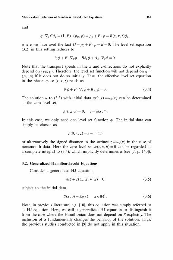
In this case, the solution S remains smooth for all time, takingthe form

S(x, t)= x2

2(t+1).

Figure 3 shows the results of our algorithm in xz-space, project-ing away p, on this problem. The initial parabola flattens out astime increases but no multi-valuedness occurs.

(2) Case—Focusing at a Point

S0(x)=−x2

2, x ∈ IR.

In this case, all rays intersect at the focus point (x, Tc)= (0,1),and then spread out afterwards. Thus almost everywhere inspace, there is a single-valued phase, taking the form

S(x, t)= x2

2(t−1).

–2.5 –2 –1.5 –1 –0.5 0 0.5 1 1.5 2 2.5–2.5

–2

–1.5

–1

0

0.5

1

1.5

2

2.5

–0.5

Fig. 3. Our approach for free motion on an initial parabola, the one above the rest. No sin-gularities appear in this example. The plots are at time intervals of 0.167318 with the finalcurve at time 2.00781.


Figure 4 shows our projected results in xz-space for this exam-ple. The initially inverted parabola becomes thinner and thinner,eventually flipping over to parabolas lying above the x-axis andexpanding. Some of the parabolas are “cut off” in the graph dueto the finite z-direction of the domain used in our computations.

(3) Case—Caustic

S0(x)=− ln(cosh(x)), x ∈ IR.

In this case, a singularity appears at time 1 and located at x=0. After this time and from this location, a multi-valued phaseappears. Figure 5 shows the behavior of the solution obtainedfrom our algorithm plotted at equal time intervals up to time1.5. The shrinking solutions develop a swallow-tail singularityafter the critical time Tc=1 at x=0. A zoom of specifically thismulti-valuedness between time 1 and 1.5 are also shown in thefigure. These results fit with the analysis of the PDE.

–1 –0.8 –0.6 –0.4 –0.2 0 0.2 0.4 0.6 0.8 1–1

–0.8

–0.6

–0.4

–0.2

0

0.2

0.4

0.6

0.8

1

Fig. 4. Our approach showing focusing on an initial inverted parabola, the uppermost con-cave down one. The parabola remains concave down and adds curvature before the singu-larity, afterwhich it switches to concave up and relaxing in curvature. The plots are at timeintervals of 0.1669248 with the final curve at time 2.0031.


–1.5 –1 –0.5 0 0.5 1 1.5–1.5

–1

–0.5

0

0.5

1

1.5

–0.2 0 0.2

–0.2

0

0.2

Fig. 5. Our approach capturing caustics, with a swallow-tail multi-valuedness developing atthe critical time with initial curve the uppermost concave down parabola. The plots are attime intervals of 0.1673176 with the final curve at time 1.50586. The figure on the right is azoomed picture around the singularity of the solutions at and after the critical time.

Example 4—Harmonic oscillator V (x)=x2/2For general V (x), the level set evolution equation takes the form

∂tφ+p∂xφ+(p2

2−V (x)

)∂zφ− ∂xV (x)∂pφ=0

and the initial data can in many cases be taken as

φ1(0)= z−S0(x), φ2(0)=p− ∂xS0(x).

For V (x)=x2/2 and S0(x)=x (see [32]), rays will intersect at the focalpoints

(x, Tc)=((−1)m+1,

(2m+1)π2

), m∈ZZ.

The solution in fact is explicitly given as

S(x, t)=−12(x2 +1) tan(t)+ x

cos(t), t �= (2m+1)π

2.

Figure 6 shows our results, plotted in xz-space, for this problem. The ini-tial line z=x first focuses at x=1 and then subsequently at x=−1, at eachtime developing multi-valuedness after the focusing. This oscillation con-tinues since the singularties form periodic in time. Although there are once


–2.5 –2 –1.5 –1 –0.5 0 0.5 1 1.5 2 2.5–2.5

–2

–1.5

–1

–0.5

0

0.5

1

1.5

2

1

Fig. 6. Our approach for the harmonic oscillator showing oscillating focusing effects occur-ing between two points. The inital curve is the line through the origin of slope 1. This sub-sequently bends into concave down parabolas, then concave up ones about the singularity onthe right. In later time these straighten out to a line of slope −1 and reproduce the behav-ior about the singularity on the left. The plots are at time intervals of 0.333484 with the finalcurve at time 10.0045.

again “cut offs” due to the computational domain used, we are still ableto capture the multi-valued solution throughout the focusing effects.

Example 6—Other multi-valued phenomenaIn the semiclassical limit for plasma, there appears the equation

St + |Sx |22

=−αS

with S0(x)= −|x| and some physical parameter α > 0. With x ∈ IR1 andα=1, we plot the results in Fig. 7 along with branches of the exact solu-tion at the final time. These branches satisfy −(|x| + t)e−t + 0.5(1 − e−t )for |x|> t , and (±|x| − t)e−t + 0.5(1 − e−t ) or 0.5x2(1 − e−t )/t2 for |x| ≤t . The multi-valued characteristics match and the positions are in goodagreement except for the small, thin loops at the ends of the swallow-tails,whose lengths are cut by half in the computed solution. This may be dueto numerical diffusion and resolution with the nonsmooth initial data.


–0.5 –0.4 –0.3 –0.2 –0.1 0 0.1 0.2 0.3 0.4 0.5 –0.5 –0.4 –0.3 –0.2 –0.1 0 0.1 0.2 0.3 0.4 0.5–0.5

–0.4

–0.3

–0.2

–0.1

0

0.1

0.2

0.3

0.4

0.5

–0.5

–0.4

–0.3

–0.2

–0.1

0

0.1

0.2

0.3

0.4

0.5

Fig. 7. Our approach applied in the semiclassical limit for plasma is shown. The initialcurve, the inverted V-shape, develops a swallow-tail with small, thin loops at the ends. Theplots are at time intervals of 0.888888 with the final curve at time 0.444444. The figure onthe right shows branches of the exact solution with the same characteristics as in the com-puted solution.

ACKNOWLEDGMENTS

Liu’s research was supported in part by the National Science Founda-tion under Grant DMS05-05975, Cheng’s research was supported in partby NSF grant #0208449 and Osher’s research was supported by AFOSRGrant F49620-01-1-0189.

REFERENCES

1. Benamou, J. D., Castella, F., Katsaounis T., and Perthame, B. (2001). High-frequencyHelmholtz Equation, Geometrical Optics and Particle Methods, Revist. Math. Iberoam.

2. Benamou, J.-D. (1996). Big ray tracing: multivalued travel time field computation usingviscosity solution of the eikonal equation. J. Comp. Phys., 128, 463–474.

3. Benamou, J. D. (1999). Direct solution of multivalued phase space solutions for Hamil-ton-Jacobi equations. Comm. Pure Appl. math., 52, 1443–1475.

4. Brenier, Y. (1984). Averaged multivalued solutions for scalar conservation laws. SIAM J.Numer. Anal. 21, 1013–1037.

5. Brenier, Y., and Corrias, L. (1998). A kinetic formulation for multi-branch entropy solu-tions of scalar conservation laws. Ann. Inst. Henri Poincare 15, 169–190.

6. Burchard, P., Cheng, L.-T., Merriman, B., and Osher, S. (2001). Motion of curves inthree spatial dimensions using a level set approach. J. Comput. Phys. 170, 720–741.

7. Courant, R,. and Hilbert, D. (1952–1962). Methods of Mathematical Physics, Vol 2, In-terscience Publishers, New York.

8. Cheng, L.-T., Osher, S., Kang, M., Shim, H., and Tsai, Y.-H. Reflection in a level setframework for geometric optics. Comp. Methods Eng. Phys. to appear.

9. Cheng, L.-T., Liu, H.-L., and Osher, S. (2003). Computational high-frequency wave prop-agation in Schodinger equations using the Level Set Method, with applications to thesemi-classical limit of Schrodinger equations. Comm. Math. Sci. 1(3), 593–621.


10. Crandall, M., and Lions, P. L. (1984). Viscosity solutions of Hamilton-Jacobi equations.Trans. AM. Math. Soc. 282, 487.

11. Engquist, B., Fatemi, E., and Osher, S. (1995). Numerical solution of the high frequencyasymptotic expansion for the scalar wave equation. J. Comput. Phys. 120, 145–155.

12. Engquist, B., and Runborg, O. (1996). Multi-phase computations in geometrical opticsJ. Comp. Appl. Math. 74, 175–1992.

13. Engquist, B., Runborg, O. and Tornberg, T.-K. (2002). High frequency wave propagationby the segment projection method. J. Comput. Phys. 178, 373–390.

14. Engquist, B., and Runborg, O. (2003). Computational high frequency wave propagation,Acta Numerica, 2003.

15. Evans, L.-C. (1996). A geometric interpretation of the heat equation with multi-valuedinitial data. SIAM J. Math. Anal. 27, 932–958.

16. Gosse, L. (2002). Using K-branch entropy solutions for multivalued geometric opticscomputations. J. Comp. Phys., 180, 155–182.

17. Gosse, L., Jin, S., and Li, X. (2003). On two moment systems for computing multi-phase semiclassical limits of the Schrodinger equation. Math. Models Methods Appl. Sci.13(12), 1689–1723.

18. Gray, S., and May, W. (1994). Kirchhoff migration using eikonal equation travel times.Geophysics, 59, 810–817.

19. Gasser, I., and Markowich, P. A. (1997). Quantum hydrodynamics, Wigner transformand the classical limit. Asymptotic Anal. 14, 97–116.

20. Gerard, P., Markowich, P. A., Mauser, N. J., and Poupaud, F. (1997). Homogenizationlimits and Wigner transforms. Comm. Pure Appl. Math. 50, 323–380.

21. Jin, S., and X. Li, Multi-phase computations of the semiclassical limit of the Schrodingerequation and related problems: Whitham vs Wigner. Physics D. 182 (2003), no. (1–2),46–85.

22. Jin, S., and Osher, S. A level set method for the computation of multivalued solutionsto quasi-linear hyperbolic PDE’s and Hamilton-Jacobi equations. submitted to Comm.Math. Sci.

23. Liu, H. Geometrical solutions of Hamilton-Jacobi equations, preprint (2004).24. Min, C. (2003). Simplicial isosurfacing in arbitrary dimension and codimension. J. Com-

put. Phys. 190, 295–310.25. Min, C. (2004). Local level set method in high dimension and codimension. J. Comput.

Phys. 200, 368–382.26. Osher, S. (1993). A level set formulation for the solution of the Dirichlet problem for

Hamilton-Jacobi equations. SIAM J. Math. Anal. 24, 1145–1152.27. Osher, S., Cheng, L.-T., Kang, M., Shim, H., and Tsai, Y.-H. (2002). Geometric optics in

a phase space based level set and eulerian framework. J. Comput. Phys. 179, 622–648.28. Osher, S., and Fedkiw, R., Level Set Method and Dynamic Implicit Surfaces. Springer-

Verlag, NY.29. Osher, S., and Sethian, J. (1988). Fronts propagating with curvature dependent speed:

algorithms based on Hamilton-Jacobi formulations. J. Comput. Phys. 79, 12–49.30. Qian, J., Cheng, L.-T., and Osher, S. (2003). A level set based Eulerian approach for

anisotropic wave propagation. Wave Motion 37, 365–379.31. Runborg, O. (2000). Some new results in multi-phase geometric optics. Math. Model.

Num. Anal. 34, 1203–1231.32. Sparber, C., Markowich, P. A., and Mauser, N. J. (2003). Wigner functions versus WKB-

methods in multivalued geometrical optics. Asymptot. Anal. 33(2), 153–187.


33. Tsai, Y.-H. R., Giga, Y., and Osher, S. (2003). A level set approach for computing dis-continuous solutions of Hamilton-Jacobi equations. Math. Comp. 72, 159–181.

34. Whitham, G. B. (1974). Linear and Nonlinear Waves, Wiley-Interscience [John Wiley &Sons], New York.

a level set framework for capturing multi-valued solutions of

Documents