A Lesson in Business ProcessSimulation Modeling

Created by

Richard Born

Associate Professor Emeritus

Northern Illinois University

richb@rborn.org

Topics

Probability and Statistics

Modeling

Robotics

Ages

Grades 11 through College

Duration

approx. 75 minutes

OZO

BOT STREA

M

APPROVED

1" !!!!!!!!!!!!!!!!!!!!!!!!!!!!!!!!!!!!!!!!!!!!!!!!!!!!!!!!!!!!!!!!!!!!!!!!!!!!!!!!!!!!!!!!!!!!!!!!!!!!!!!!!!!!!!!!!!!!!!!!!!!!©!2015!Richard!G.!Born!

!

A LESSON IN BUSINESS PROCESS SIMULATION MODELING

TEACHER’S GUIDE

What will students learn?

• What is simulation modeling? • How can simulation modeling be used to understand and improve business

processes? • What are some examples of business processes involving randomness? • How can Ozobot be used to simulate random business processes? • What are the advantages of using a computer over Ozobot to simulate

random processes? • How can Blockly be used to generate random numbers to simulate business

processes? • What does the JavaScript code look like that is created automatically from

a Blockly program?

Business Process Simulation Modeling

Let’s work in reverse by starting with the word modeling. Modeling involves building a simplified “picture” of an existing or proposed system. For example, you might want to model the operation of your grocery store from the initial arrival of customers to their final checkout just before leaving the store. To improve the overall customer experience by reducing waiting time, you may want to model your store with some proposed additional checkout counters.

Simulation involves doing experiments with the model of an existing or proposed system. You can accomplish this by systematically varying input data and study its effect on output data. In our grocery store example, input data could be the interarrival time of customers and the number of items in their carts. Output data could be waiting time at the checkout counter. Your simulation could vary the arrival rate of customers and how full the customer’s carts are, and study their effect on waiting time at the checkout counters. You could also study the effect on waiting time of adding one, two, or more additional checkout counters. The primary advantage of doing this via simulation is that you can

2" !!!!!!!!!!!!!!!!!!!!!!!!!!!!!!!!!!!!!!!!!!!!!!!!!!!!!!!!!!!!!!!!!!!!!!!!!!!!!!!!!!!!!!!!!!!!!!!!!!!!!!!!!!!!!!!!!!!!!!!!!!!!©!2015!Richard!G.!Born!

!

investigate the consequences of these different decisions before investing money in building the additional checkout counters.

Finally, what is meant by business processes? Business processes are events that follow active entities including customers, clerks, and baggers. In our grocery store model, events include interarrivals of customers, a customer removing an item from a shelf and placing it in his or her cart, a customer unloading the cart at the checkout counter, the clerk scanning the items, the bagger bagging the purchases, and the customer making payment before exiting the store. Many of these business processes involve randomness. Customers arrive with random interarrival times. Customers place items in their carts at random times as they traverse the aisles in the grocery store. Different customers unload their carts at random rates that vary from one customer to another. The time that customers wait in line at checkout counters is random output of the business processes.

These random business processes occur at discrete points in time. For example, the first customer may arrive at 5 minutes after the grocery store opens, the second customer at 9 minutes after opening, the third customer at 15 minutes after opening, and-so-on. Because these business processes occur at discrete points in time, simulation of such processes is often called discrete-event simulation. In discrete-event simulation, the simulation clock moves between the occurrences of events that cause noticeable changes in the states of system components.

It should be clear by now that the generation of random numbers is essential for performing business process simulation modeling. In this lesson we will use Ozobot to generate random numbers to help in solving an interesting business-related problem. Toward the end of this lesson, we will also see how to use Google’s Blockly and JavaScript as alternatives to Ozobot for generating random numbers.

A reasonable simulation solution could be seen as involving five steps: problem formulation, data collection and analysis, model development, model experimentation, and output analysis.

Step 1: Problem Formulation—Our Business Problem

A local community radio station occasionally runs telethons to raise money for residents who have a special need or have experienced a tragedy such as home damage due to fire or flood. The radio station has just decided to run a telethon

3" !!!!!!!!!!!!!!!!!!!!!!!!!!!!!!!!!!!!!!!!!!!!!!!!!!!!!!!!!!!!!!!!!!!!!!!!!!!!!!!!!!!!!!!!!!!!!!!!!!!!!!!!!!!!!!!!!!!!!!!!!!!!©!2015!Richard!G.!Born!

!

to help in raising money to send the high school orchestra to a national competition for which they have just qualified

In past telethons, the radio station has had one agent devoted to handling incoming pledge calls, but is now considering having two agents. It is hoped that with two agents handling calls, the total revenue generated will increase since there will be fewer lost calls due to the line being busy when someone calls in with a pledge. The radio station is not set up for call queuing, so if the line is busy, the caller must hang up—the call is lost.

Management of the radio station would like to know several things before proceeding with the telethon:

• How many pledges will be made? • How much revenue will be generated by the telethon? • How many pledges will be lost because all lines are busy when the call is

made? • What is the utilization for each of the agents? Utilization is the

percentage of time that the agent is busy handling calls. • Should there be one or two agents handling incoming pledge calls?

The simulation model that we design must allow us to answer the above five questions, so they must be kept in mind throughout our work.

Step 2: Data Collection and Analysis

With the problem now defined, we can begin looking at things related to data collection and analysis. In order to drive the simulation, there are three kinds of data that need to be gathered:

• Call duration data—the time that an agent spends on the telephone with individuals making a pledge.

• Call interarrival time data—the time interval between one pledge call and the next.

• Pledge amount in dollars for each caller.

Regarding call duration, we’ll assume that the radio station has kept detailed records of call duration for past telethons. They have found that call-duration is randomly and uniformly distributed between 3 and 10 minutes, as depicted in the figure at the top of the next page.

4" !!!!!!!!!!!!!!!!!!!!!!!!!!!!!!!!!!!!!!!!!!!!!!!!!!!!!!!!!!!!!!!!!!!!!!!!!!!!!!!!!!!!!!!!!!!!!!!!!!!!!!!!!!!!!!!!!!!!!!!!!!!!©!2015!Richard!G.!Born!

!

Regarding call interarrival times, the radio station has also kept detailed records for past telethons. They have found that call interarrival times are randomly and uniformly distributed between 1 and 6 minutes, as depicted in this figure:

Finally, the radio station records from past telethons have revealed that the pledge amount varies randomly with a “triangular” shaped distribution similar to that shown below. The smallest pledge is about $20 with low probability. The peak probability for pledges occurs at $70. The maximum pledge occurs at about $120, but with low probability.

5" !!!!!!!!!!!!!!!!!!!!!!!!!!!!!!!!!!!!!!!!!!!!!!!!!!!!!!!!!!!!!!!!!!!!!!!!!!!!!!!!!!!!!!!!!!!!!!!!!!!!!!!!!!!!!!!!!!!!!!!!!!!!©!2015!Richard!G.!Born!

!

Step 3: Model Development

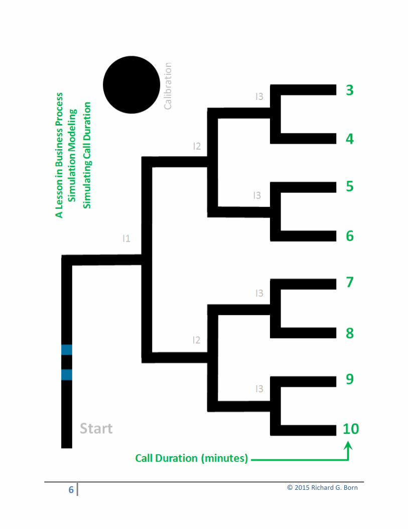
Now that we have completed the data collection and analysis step, we can move on to model development. The technology that we will use to generate the required random numbers is Ozobot. This is possible because Ozobot has been designed to make independent routing decisions at intersections based upon algorithms involving random logic. Independent routing decisions means that the decision it makes at one intersection “has nothing to do” with the decision it makes later at the same intersection or another intersection.

First we address how Ozobot can be used to simulate call duration. The left side of the figure below reminds us that we want call durations to be uniformly and randomly distributed between 3 and 10 minutes. If we are willing to simplify our model to generate whole number call duration times, then the right side of the figure below shows that we want eight possible random call durations varying from 3 through 10 minutes. An OzoMap that accomplishes this is shown on page 6. The Blue-Black-Blue Ozocode shortly after the start simply speeds up Ozobot to make data collection quicker.

When Ozobot reaches the first intersection (I1), the probability is ½ for each direction it takes there. For the second intersection (I2), the probability is again ½. Similarly, the probability is ½ for each direction taken at the third intersection (I3). Since these three events are independent, the probability for arriving at any of the eight call durations from 3 through 10 minutes is the product of the probabilities: ½ x ½ x ½ = 1/8.

Our simplified model does not allow call duration times of, say, 4.6 minutes or 9.2 minutes. It only allows for call durations that are a whole number of minutes. There are tradeoffs between producing an exact representation of the real system and our more simplified model.

6" !!!!!!!!!!!!!!!!!!!!!!!!!!!!!!!!!!!!!!!!!!!!!!!!!!!!!!!!!!!!!!!!!!!!!!!!!!!!!!!!!!!!!!!!!!!!!!!!!!!!!!!!!!!!!!!!!!!!!!!!!!!!©!2015!Richard!G.!Born!

!

7" !!!!!!!!!!!!!!!!!!!!!!!!!!!!!!!!!!!!!!!!!!!!!!!!!!!!!!!!!!!!!!!!!!!!!!!!!!!!!!!!!!!!!!!!!!!!!!!!!!!!!!!!!!!!!!!!!!!!!!!!!!!!©!2015!Richard!G.!Born!

!

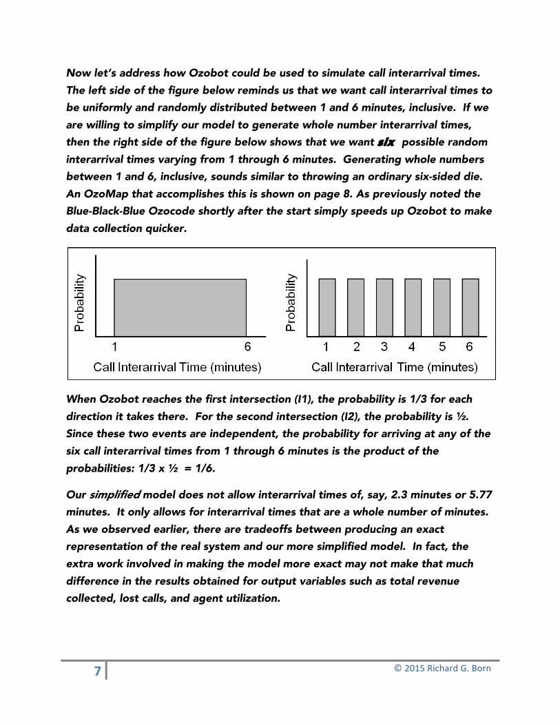
Now let’s address how Ozobot could be used to simulate call interarrival times. The left side of the figure below reminds us that we want call interarrival times to be uniformly and randomly distributed between 1 and 6 minutes, inclusive. If we are willing to simplify our model to generate whole number interarrival times, then the right side of the figure below shows that we want six possible random interarrival times varying from 1 through 6 minutes. Generating whole numbers between 1 and 6, inclusive, sounds similar to throwing an ordinary six-sided die. An OzoMap that accomplishes this is shown on page 8. As previously noted the Blue-Black-Blue Ozocode shortly after the start simply speeds up Ozobot to make data collection quicker.

When Ozobot reaches the first intersection (I1), the probability is 1/3 for each direction it takes there. For the second intersection (I2), the probability is ½. Since these two events are independent, the probability for arriving at any of the six call interarrival times from 1 through 6 minutes is the product of the probabilities: 1/3 x ½ = 1/6.

Our simplified model does not allow interarrival times of, say, 2.3 minutes or 5.77 minutes. It only allows for interarrival times that are a whole number of minutes. As we observed earlier, there are tradeoffs between producing an exact representation of the real system and our more simplified model. In fact, the extra work involved in making the model more exact may not make that much difference in the results obtained for output variables such as total revenue collected, lost calls, and agent utilization.

8" !!!!!!!!!!!!!!!!!!!!!!!!!!!!!!!!!!!!!!!!!!!!!!!!!!!!!!!!!!!!!!!!!!!!!!!!!!!!!!!!!!!!!!!!!!!!!!!!!!!!!!!!!!!!!!!!!!!!!!!!!!!!©!2015!Richard!G.!Born!

!

9" !!!!!!!!!!!!!!!!!!!!!!!!!!!!!!!!!!!!!!!!!!!!!!!!!!!!!!!!!!!!!!!!!!!!!!!!!!!!!!!!!!!!!!!!!!!!!!!!!!!!!!!!!!!!!!!!!!!!!!!!!!!!©!2015!Richard!G.!Born!

!

Lastly, we need to address how Ozobot could be used to simulate pledge amounts. The left side of the figure below reminds us that we want the pledge amounts to be randomly and “triangularly” distributed between $20 and $120, with peak probability occurring at a pledge of $70. The right side of the figure below shows the long-term, expected “triangular” distribution obtained by rolling a pair of ordinary six-sided dice and summing the faces up. This distribution is triangular shaped peaking at 7, which can be obtained by rolling (1,6), (6,1), (5,2), (2,5), (3,4), and (4,3). A sum of 2 is obtained only by rolling (1,1), and a sum of 12 is obtained only by rolling (6,6). If we roll a pair of dice and the multiply the sum by 10, we will have numbers between 20 and 120, with a peak probability occurring at a sum of 70. This is just what we need to simulate the pledge amounts!

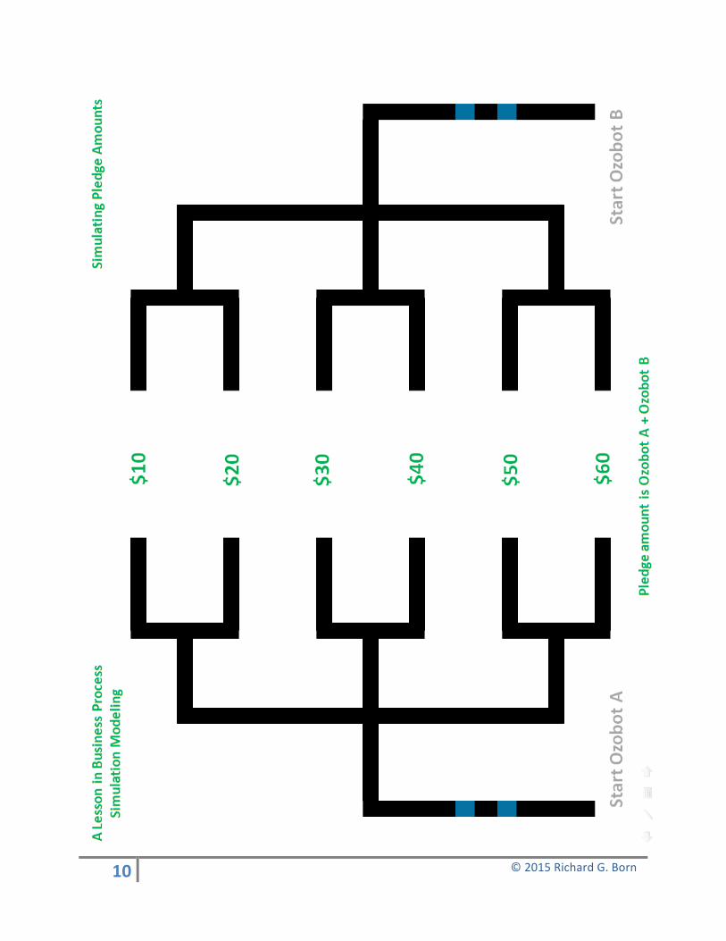
The OzoMap shown on page 10 can be used to simulate the pledge amount for each caller. The map consists of two separate maps similar to the OzoMap on page 8. Each of the maps simulates rolling a single die. The result of Ozobot’s traversal of these maps results in dollar amounts from $10 to $60, with equal probabilities for each amount. If Ozobot on the left map landed at $30 and Ozobot on the right map landed on $50, then this would represent a pledge amount of $30 + $50 = $80 for the simulation.

The data has admittedly been contrived to simplify mental calculations and the recording of data later during model experimentation, but this in no way invalidates what the class is learning about the steps involved in a simulation project. Actual simulation modeling software is not limiting in the way that physical devices such as dice and Ozobot are. But the use of dice or Ozobot allows the student to concentrate on how simulation modeling is done, as they do not hide the details that actual simulation software hides.

10" !!!!!!!!!!!!!!!!!!!!!!!!!!!!!!!!!!!!!!!!!!!!!!!!!!!!!!!!!!!!!!!!!!!!!!!!!!!!!!!!!!!!!!!!!!!!!!!!!!!!!!!!!!!!!!!!!!!!!!!!!!!!©!2015!Richard!G.!Born!

!

11" !!!!!!!!!!!!!!!!!!!!!!!!!!!!!!!!!!!!!!!!!!!!!!!!!!!!!!!!!!!!!!!!!!!!!!!!!!!!!!!!!!!!!!!!!!!!!!!!!!!!!!!!!!!!!!!!!!!!!!!!!!!!©!2015!Richard!G.!Born!

!

In our model, we assume that if all agents are busy, then the customer will hang up and not call back later. We could allow callback after a predetermined period of time, and we could even allow for call queuing, but agree for the sake of simplicity not to model either of these things at this time. It should be pointed out, however, that modeling callback as well as call queuing would be quite straight forward with the use of simulation software. We note that, as a tie breaker, a customer calling in will be assigned to the lowest numbered available agent if more than one agent is available to take the call.

Finally, with regard to model development, we agree to simulate the telethon for one hour of system operation. We further realize that we must collect data that will allow tracking of the following items:

• The number of pledges made • The pledge amount for each pledge made • The number of calls lost because all agents are busy when a call arrives • The utilization of each agent

The basic physical flow for our system is as follows:

• A caller places a call to make a pledge to the telethon. • If all agents are busy, the caller hangs up. • If agents are available, the caller is assigned to the lowest numbered agent. • The pledge is recorded by the agent. • The caller hangs up after making his/her pledge.

Step 4: Model Experimentation

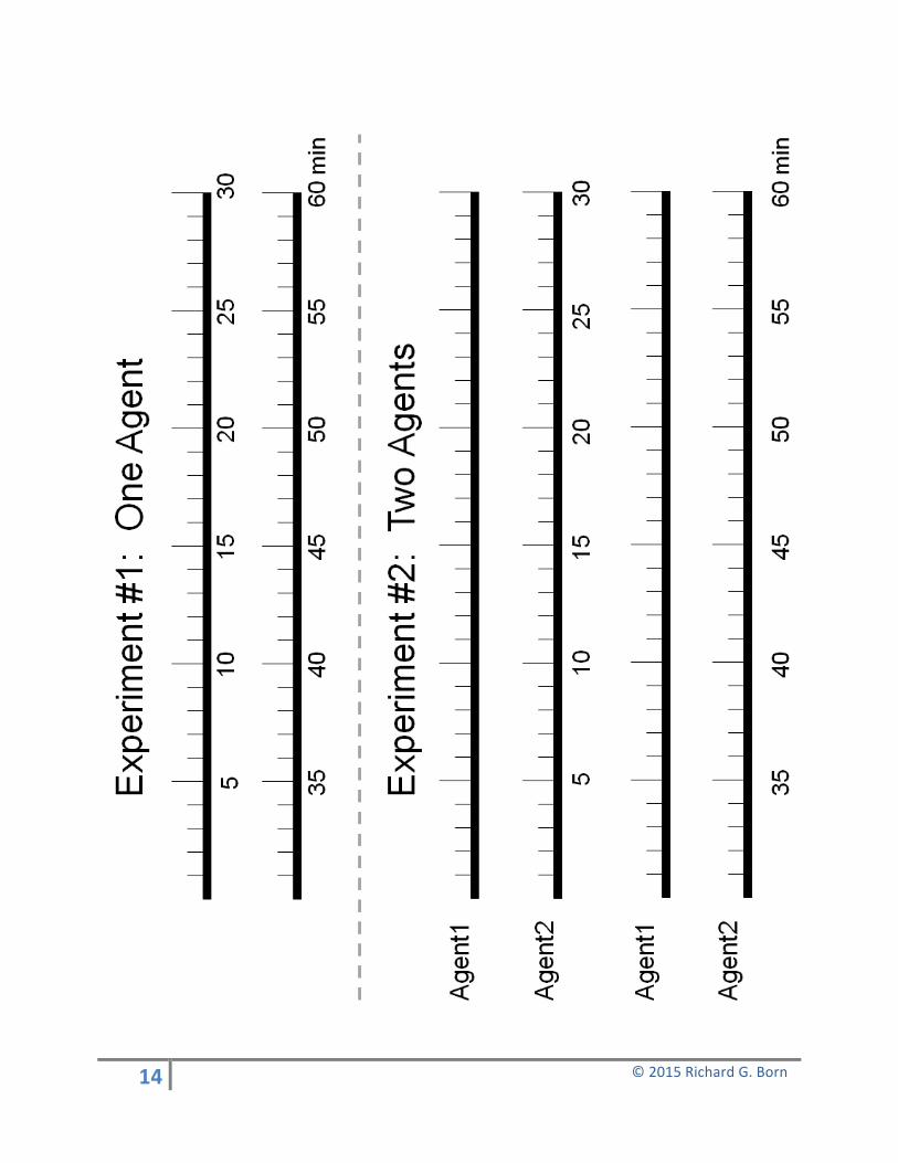
We are finally ready to do the simulation experiment. It is recommended to have the entire class do the experiment once together with the instructor’s guidance to make sure that everyone understands how to go about collecting the data during the experiment. Ozobot generated random number data sheets are provided for each student to record result as shown on page 13. From these data sheets, the student can then construct the simulation time-line sheet shown on page 14. The class usually understands why they need to do two experiments, i.e., one experiment in which there is one agent answering calls and one in which there are

12" !!!!!!!!!!!!!!!!!!!!!!!!!!!!!!!!!!!!!!!!!!!!!!!!!!!!!!!!!!!!!!!!!!!!!!!!!!!!!!!!!!!!!!!!!!!!!!!!!!!!!!!!!!!!!!!!!!!!!!!!!!!!©!2015!Richard!G.!Born!

!

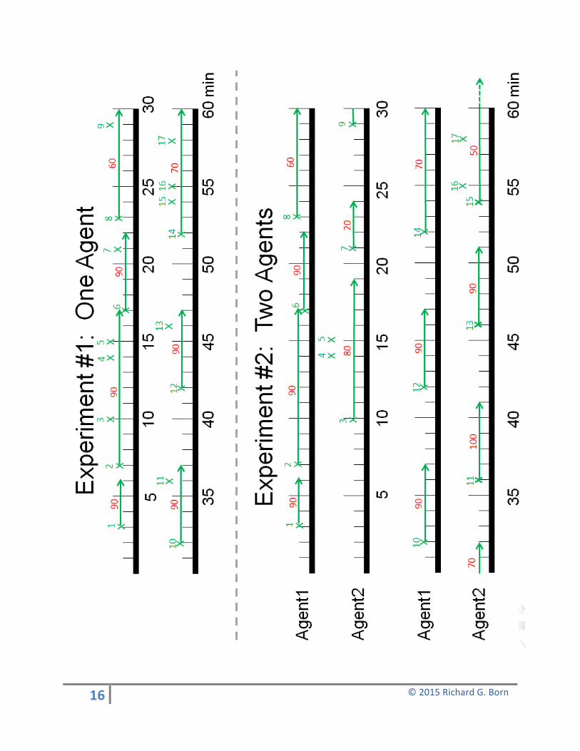
two agents. But the instructor must point out that we need to apply the same random input data to both experiments. When asked why, someone in the class may respond by saying that it is important that we have the same sequence of call interarrivals, call durations, and pledge amounts for both experiments. If the results are different for the two experiments, then we have good reason to believe that the results differ because the number of agents differs. This can lead to a good discussion of the need to control variables in an experiment. See an example Ozobot generated list of random numbers on page 15 and the corresponding completely filled in timeline data sheet for the experiment shown on page 16. On the timeline chart call arrivals are indicated by marking an X at the appropriate place on the timeline. An arrow whose length indicates the random call duration in minutes is then drawn to the right of the X. If the call is a lost call, the X will appear without the arrow to its right. The pledge amount for each of the calls is recorded above its corresponding arrow in red. The numbers in green above each X are caller numbers—1st caller, 2nd caller, 3rd caller, etc. When getting near the end of the experiment, the students often find that the arrow goes beyond 60 minutes, meaning that the call is not completed during the hour simulated. They then need to agree on how to handle the pledge amount for this particular call. It is suggested that the pledge amount be included in those for the hour simulated. Finally, they realize that the experiment has ended when the random interarrival time generated by Ozobot would place a call after the simulation hour has elapsed. Having completed the experiments once as a class under the guidance of the teacher, students can then break up into groups and perform the experiments again with each group using its own Ozobots. Group results can then be averaged, as will be discussed later in the section on output analysis. In order to get some meaningful averages, it is desirable to have at least six groups doing the experiments. One of the cardinal rules of discrete-event simulation modeling is to never base recommendations to management on only a single simulation run of your model. Page 17 contains a detailed discussion of how the time-line data sheet on page 16 with its X’s and arrows is constructed from the data table on page 15.

13" !!!!!!!!!!!!!!!!!!!!!!!!!!!!!!!!!!!!!!!!!!!!!!!!!!!!!!!!!!!!!!!!!!!!!!!!!!!!!!!!!!!!!!!!!!!!!!!!!!!!!!!!!!!!!!!!!!!!!!!!!!!!©!2015!Richard!G.!Born!

!

Table of Ozobot Generated Random Numbers for the Telethon Simulation

Caller Number Interarrival Time (Minutes)

Call Duration (minutes)

Pledge Amount ($)

1 2 3 4 5 6 7 8 9 10 11 12 13 14 15 16 17 18 19 20 21 22 23 24 25

14" !!!!!!!!!!!!!!!!!!!!!!!!!!!!!!!!!!!!!!!!!!!!!!!!!!!!!!!!!!!!!!!!!!!!!!!!!!!!!!!!!!!!!!!!!!!!!!!!!!!!!!!!!!!!!!!!!!!!!!!!!!!!©!2015!Richard!G.!Born!

!

15" !!!!!!!!!!!!!!!!!!!!!!!!!!!!!!!!!!!!!!!!!!!!!!!!!!!!!!!!!!!!!!!!!!!!!!!!!!!!!!!!!!!!!!!!!!!!!!!!!!!!!!!!!!!!!!!!!!!!!!!!!!!!©!2015!Richard!G.!Born!

!

Example Table of Ozobot Generated Random Numbers

Caller Number Interarrival Time (Minutes)

Call Duration (minutes)

Pledge Amount ($)

1 3 3 90

2 4 10 90

3 3 9 80

4 4 8 80

5 1 7 80

6 2 5 90

7 4 3 20

8 2 7 60

9 6 3 70

10 3 5 90

11 4 5 100

12 6 5 90

13 4 5 90

14 6 8 70

15 2 8 50

16 1 8 70

17 3 5 50

18 4 3 60

16" !!!!!!!!!!!!!!!!!!!!!!!!!!!!!!!!!!!!!!!!!!!!!!!!!!!!!!!!!!!!!!!!!!!!!!!!!!!!!!!!!!!!!!!!!!!!!!!!!!!!!!!!!!!!!!!!!!!!!!!!!!!!©!2015!Richard!G.!Born!

!

17" !!!!!!!!!!!!!!!!!!!!!!!!!!!!!!!!!!!!!!!!!!!!!!!!!!!!!!!!!!!!!!!!!!!!!!!!!!!!!!!!!!!!!!!!!!!!!!!!!!!!!!!!!!!!!!!!!!!!!!!!!!!!©!2015!Richard!G.!Born!

!

It may be helpful to the reader if we provide an explanation of how to fill out the timelines for the first few callers. This will now be done for the Ozobot data on page 15 and the corresponding timeline on page 16. It is suggested that both of these pages be in view during the discussion that follows.

Experiment #1: One Agent

Caller Number 1: The interarrival time is 3 minutes; therefore an X is placed at the 3-minute mark on the timeline and the caller number 1 is written above the X. The call duration is 3 minutes; therefore an arrowed segment is drawn from the 3 to the 6 minute marks. The pledge amount is $90; therefore 90 is written above the arrowed segment.

Caller Number 2: The interarrival time is 4 minutes. This means that the call arrives 4 minutes after the previous call; therefore an X is placed at 3+4=7 minutes to indicate the call arrival. The caller number 2 is written above the X. The call duration is 10 minutes; therefore an arrowed segment is drawn from 7 to 17 minutes. The pledge amount is again $90; therefore 90 is written above the arrowed segment.

Caller Number 3: The interarrival time is 3 minutes. This means that the call arrives at 7+3=10 minutes. Since the agent is busy, the caller must hang up and we have a lost call. To indicate that the call is lost, we write an X at the call arrival time of 10 minutes and the caller number 3 is written above the X.

This process continues until the entire timeline has been filled out. The simulation stops with caller number 18 because the call arrival time is beyond the end of the simulation time of 1 hour (60 minutes).

Experiment #2: Two Agent

Caller Number 1: The interarrival time is 3 minutes; therefore an X is placed at the 3-minute mark on the timeline for agent 1 and the caller number 1 is written above the X. (Remember that we agreed to assign calls to the lowest numbered agent if more than one agent is free.) The call duration is 3 minutes; therefore an arrowed segment is drawn from the 3 to the 6 minute marks. The pledge amount is $90; therefore 90 is written above the arrowed segment.

18" !!!!!!!!!!!!!!!!!!!!!!!!!!!!!!!!!!!!!!!!!!!!!!!!!!!!!!!!!!!!!!!!!!!!!!!!!!!!!!!!!!!!!!!!!!!!!!!!!!!!!!!!!!!!!!!!!!!!!!!!!!!!©!2015!Richard!G.!Born!

!

Caller Number 2: The interarrival time is 4 minutes. This means that the call arrives 4 minutes after the previous call; therefore an X is placed at 3+4=7 minutes on the timeline for agent 1 to indicate the call arrival. The caller number 2 is written above the X. The call duration is 10 minutes; therefore an arrowed segment is drawn from 7 to 17 minutes. The pledge amount is again $90; therefore 90 is written above the arrowed segment.

Caller Number 3: Since agent 1 is busy and agent 2 is free, this call is assigned to agent 2. The interarrival time is 3 minutes; therefore an X is written at the 7+3=10 minute mark on the timeline for agent 2. The caller number 3 is written above the X. Since the call duration is 9 minutes, an arrowed line segment is drawn from 10 to 19 minutes. Since the pledge amount is $80, the number 80 is written above the arrow.

Caller Number 4: The interarrival time is 4 minutes. This means that the call arrives at 10+4=14 minutes. Both agents are already busy, with agent 1 handling caller number 2 and agent 2 handling caller number 3. Therefore the caller must hang up and we have a lost call. To indicate the lost call, we place an X at its 14 minute arrival time, and write the caller number 4 above the X.

This process continues until the timelines for both agents have been completed. The simulation stops with caller number 18 because the call arrival time is beyond the end of the simulation time of 1 hour (60 minutes).

This process is admittedly tedious, but going through this once or twice helps you to understand the inner-workings of discrete-event simulation software. Discrete-event simulation software is designed to handle all of these details automatically for you. There are many discrete-event simulation software packages available in the marketplace. Some even allow you to see animations of events as they happen during the simulation. One package that has been designed specifically for business education is aGPSS—a General Purpose Simulation System+, developed by Ingolf Ståhl. The author of this lesson has collaborated with Ståhl for about 25 years, and together, we have written introductory tutorials and books on the modeling of business processes. The link at the bottom of this page provides details for anyone interested in learning more about simulation modeling with aGPSS.

+ http://agpss.com

19" !!!!!!!!!!!!!!!!!!!!!!!!!!!!!!!!!!!!!!!!!!!!!!!!!!!!!!!!!!!!!!!!!!!!!!!!!!!!!!!!!!!!!!!!!!!!!!!!!!!!!!!!!!!!!!!!!!!!!!!!!!!!©!2015!Richard!G.!Born!

!

Step 5: Output Analysis

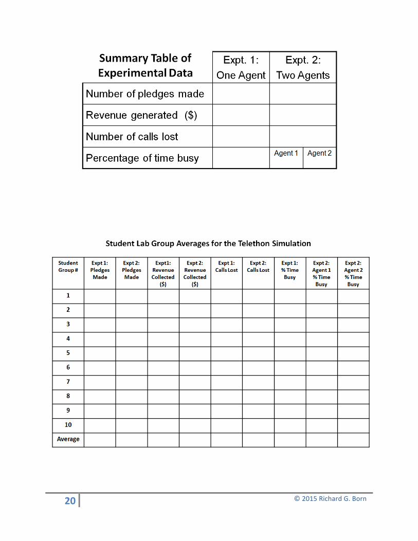
Having completed the experiments, the final step in simulation modeling is output analysis. At this point we are ready to answer the questions initially posed on page 3. Each student group is asked to complete the Summary Table of Experimental Data that appears at the top on the next page. A copy of this table is shown below, with the summary data filled in. The summary data in this table were calculated by studying the timelines on page 16.

We now explain how the summary data were obtained for the case of one agent. The method is similar for two agents.

• Number of pledges made: Simply count the number of arrowed line segments.

• Revenue generated: Add up the pledge amounts shown in red above the arrowed line segments.

• Number of calls lost: Count the number of X’s that do not have a line segment attached—they represent lost calls.

• Percentage of time busy: Count the number of minutes the agent is busy and divide by the total simulation time. 43/60 x 100% ≈ 72%.

A table is provided at the bottom of the next page to collect the summary data from each of the student lab groups and then compute averages for each of the items. From the averages, some reasonable recommendations can be made for radio station management. Recommendations will typically indicate:

• The number of pledges and revenue collected can be nearly doubled with two agents taking calls.

• The number of lost calls can be approximately halved with two agents. • Agent 2 can be assigned additional tasks since agent 2 is busy only about

50% of the time.

20" !!!!!!!!!!!!!!!!!!!!!!!!!!!!!!!!!!!!!!!!!!!!!!!!!!!!!!!!!!!!!!!!!!!!!!!!!!!!!!!!!!!!!!!!!!!!!!!!!!!!!!!!!!!!!!!!!!!!!!!!!!!!©!2015!Richard!G.!Born!

!

21" !!!!!!!!!!!!!!!!!!!!!!!!!!!!!!!!!!!!!!!!!!!!!!!!!!!!!!!!!!!!!!!!!!!!!!!!!!!!!!!!!!!!!!!!!!!!!!!!!!!!!!!!!!!!!!!!!!!!!!!!!!!!©!2015!Richard!G.!Born!

!

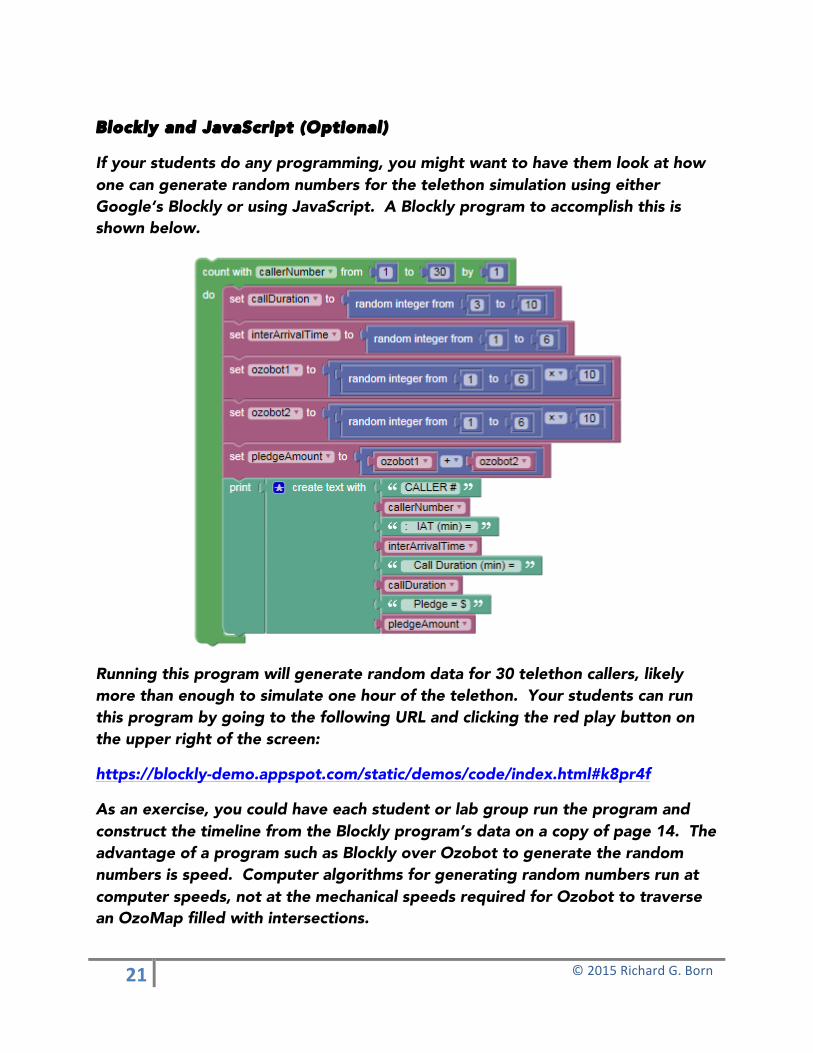
Blockly and JavaScript (Optional)

If your students do any programming, you might want to have them look at how one can generate random numbers for the telethon simulation using either Google’s Blockly or using JavaScript. A Blockly program to accomplish this is shown below.

Running this program will generate random data for 30 telethon callers, likely more than enough to simulate one hour of the telethon. Your students can run this program by going to the following URL and clicking the red play button on the upper right of the screen:

https://blockly-demo.appspot.com/static/demos/code/index.html#k8pr4f

As an exercise, you could have each student or lab group run the program and construct the timeline from the Blockly program’s data on a copy of page 14. The advantage of a program such as Blockly over Ozobot to generate the random numbers is speed. Computer algorithms for generating random numbers run at computer speeds, not at the mechanical speeds required for Ozobot to traverse an OzoMap filled with intersections.

22" !!!!!!!!!!!!!!!!!!!!!!!!!!!!!!!!!!!!!!!!!!!!!!!!!!!!!!!!!!!!!!!!!!!!!!!!!!!!!!!!!!!!!!!!!!!!!!!!!!!!!!!!!!!!!!!!!!!!!!!!!!!!©!2015!Richard!G.!Born!

!

Are your students into doing JavaScript and HTML? If so, you may want to make use of an HTML/JavaScript program that corresponds to the Blockly program to produce random numbers for the radio station’s telethon:

Your students can run this program by going to the following URL:

http://rborn.org/telethon

23" !!!!!!!!!!!!!!!!!!!!!!!!!!!!!!!!!!!!!!!!!!!!!!!!!!!!!!!!!!!!!!!!!!!!!!!!!!!!!!!!!!!!!!!!!!!!!!!!!!!!!!!!!!!!!!!!!!!!!!!!!!!!©!2015!Richard!G.!Born!

!

Suggestions for Classroom Use

Discuss the first three steps in simulation modeling with the class: Problem Formulation, Data Collection and Analysis, and Model Development, as they relate to the radio station telethon.

Then with the entire class working as a whole, go through the Model Experimentation step. One student can get the call interarrival times by using the OzoMap on page 8, another student can get the call durations by using the OzoMap on page 6, and a third student can use Ozobots on page 10 to get the pledge amounts. Each student in the class can fill out a copy of the data sheet on page 13 as the three students with the Ozobots and OzoMaps call out the random numbers generated by Ozobot. Then the teacher can help the class as a whole fill out copies of the timelines on page 14 first for Experiment 1: One Agent and then Experiment 2: Two Agents. Finally, the teacher can help the students fill out copies of the Summary of Experimental Data on page 20.

As homework, students with their own Ozobots can repeat the entire process on their own at home. If they don’t have Ozobots at home, they can make use of either the Blockly program or the HTML/JavaScript program to generate the needed random numbers. Links to these programs appear on pages 21 and 22.

During the next class period, students can record their results from their Summary of Experimental Data sheets to the Student Lab Group Averages for the Telethon data sheet. Averages can be calculated for each of the output statistics. Finally, the class can have a discussion of conclusions and recommendations that might be made to radio station management.

STEM Topics

• Interdisciplinary—robotics, math, statistics, probability, and simulation modeling working together

• Computer Science—colored visual codes are used to program a line-following robot; Blockly and JavaScript programming

• Apply domain-specific vocabulary when communicating science, technology, engineering, and mathematics concepts

• Engage in inquiry and critical thinking to solve complex business problems

24" !!!!!!!!!!!!!!!!!!!!!!!!!!!!!!!!!!!!!!!!!!!!!!!!!!!!!!!!!!!!!!!!!!!!!!!!!!!!!!!!!!!!!!!!!!!!!!!!!!!!!!!!!!!!!!!!!!!!!!!!!!!!©!2015!Richard!G.!Born!

!

Intended Grade Levels

11th through 16th Grades

Materials

Ozobots (1 per every 3 to 4 students, fully charged)

8½” x 11” bright white cardstock for printing OzoMaps on pages 6, 8, and 10 for student lab groups

Paper copies of the data sheets on pages 13, 14 and 20 for each student lab group

Estimated Time Frame

Approximately 75 minutes