a leisurely look at the bootstrap, the jackknife, and...

A Leisurely Look at the Bootstrap, the Jackknife, and Cross-ValidationAuthor(s): Bradley Efron and Gail GongSource: The American Statistician, Vol. 37, No. 1 (Feb., 1983), pp. 36-48Published by: American Statistical AssociationStable URL: http://www.jstor.org/stable/2685844 .Accessed: 04/08/2011 19:22

Your use of the JSTOR archive indicates your acceptance of the Terms & Conditions of Use, available at .http://www.jstor.org/page/info/about/policies/terms.jsp

JSTOR is a not-for-profit service that helps scholars, researchers, and students discover, use, and build upon a wide range ofcontent in a trusted digital archive. We use information technology and tools to increase productivity and facilitate new formsof scholarship. For more information about JSTOR, please contact [email protected].

American Statistical Association is collaborating with JSTOR to digitize, preserve and extend access to TheAmerican Statistician.

http://www.jstor.org

http://www.jstor.org/action/showPublisher?publisherCode=astata

http://www.jstor.org/stable/2685844?origin=JSTOR-pdf

http://www.jstor.org/page/info/about/policies/terms.jsp

A Leisurely Look at the Bootstrap, the Jackknife, and Cross-Validation

BRADLEY EFRON and GAIL GONG*

This is an invited expository article for The American Statistician. It reviews the nonparametric estimation of statistical error, mainly the bias and standard error of an estimator, or the error rate of a prediction rule. The presentation is written at a relaxed mathematical level, omitting most proofs, regularity conditions, and technical details.

KEY WORDS: Bias estimation; Variance estimation; Nonparametric standard errors; Nonparametric confidence intervals; Error rate prediction.

1. INTRODUCTION

This article is intended to cover lots of ground, but at a relaxed mathematical level that omits most proofs, regularity conditions, and technical details. The ground in question is the nonparametric estimation of statistical error. "Error" here refers mainly to the bias and standard error of an estimator, or to the error rate of a data-based prediction rule.

All of the methods we discuss share some attractive properties for the statistical practitioner: they require very little in the way of modeling, assumptions, or analysis, and can be applied in an automatic way to any situation, no matter how complicated. (We will give an example of a very complicated prediction rule indeed). An important theme of what follows is the substitution of raw computing power for theoretical analysis.

The references upon which this article is based (Efron 1979a,b, 1981a,b,c, 1982; Efron and Gong 1982) ex- plore the connections between the various nonparametric methods, and also the relationship to famil- iar parametric techniques. Needless to say, there is no danger of parametric statistics going out of business. A good parametric analysis, when appropriate, can be far more efficient than its nonparametric counterpart. Of- ten, though, parametric assumptions are difficult to justify, in which case it is reassuring to have available the comparatively crude but trustworthy nonparametric answers.

What are the bootstrap, the jackknife, and cross-

validation? For a quick answer, before we begin the main exposition, we consider a problem where none of the three methods are necessary, estimating the standard error of a sample average.

The data set consists of a random sample of size n from an unknown probability distribution F on the real line,

XI, X,, X., - F. (1)

Having observed XI = xi, X, =x, . I,= xn, we compute the sample average x- = n x,ln for use as an estimate of the expectation of F.

An interesting fact, and a crucial one for statistical applications, is that the data set provides more than the estimate x It also gives an estimate for the accuracy of x-, namely

&=:n.(n - ) X (2)

6 is the estimated standard error of X= x, the root mean squared error of estimation.

The trouble with formula (2) is that it does not, in any obvious way, extend to estimators other than X, for example the sample median. The jackknife and the bootstrap are two ways of making this extension. Let

n __ -X X1 (3) x-(,) = n - n

the sample average of the data set deleting the nth point. Also, let x(.)= = x(,)/n, the average of the deleted averages. (Actually x-(.) = x-, but we need the dot notation below.) The jackknife estimate of standard error is

&J=[n 1 (x(.))2] (4)

The reader can verify that this is the same as (2). The advantage of (4) is an easy generalizability to any estimator 0 = 6(XI, X2, . . , Xn). The only change is to substitute 6(,) = (XI, X, X+, . . ., Xn) for x-(,) and 0( ) = 0(,)n for X(.).

The bootstrap generalizes (2) in an apparently different way. Let F be the7empirical probability distribution of the data, putting probability mass l/n on each x,, and let X*, X , X* be a random sample from F,

X*,. X*2, .--, Xn_F (5)

In other words each X* is drawn independently with replacement and with equal probability from the set {xl,

... , x4. Then X = n X*,/n has variance

*Bradley Efron is Professor of Statistics and Biostatistics at Stan- ford University. Gail Gong is Assistant Professor of Statistics at Carnegie-Mellon University. The authors are grateful to Rob Tibshir- ani who suggested the final example in Section 7; to Samprit Chat- terjee and Werner Stuetzle who suggested looking at estimators like "BootAve" in Section 9; and to Dr. Peter Gregory of the Stanford Medical School who provided the original analysis as well as the data in Section 10. This work was partially supported by the National Science Foundation and the National Institutes of Health.

36 (D The American Statistician, February 1983, Vol. 37, No. I

var* X* =1 E (xi -X)2' (6) i=1

var* indicating variance under sampling scheme (5). The bootstrap estimate of standard error for an estimator 6(Xl, X2, * * , Xn) iS

as= [var. ( X2, X , X,)] (7)

Comparing (7) with (2) we see that [nl(n - 1)]1/2

&B= a for 0 = X. We could make &B exactly equal &, for 0 X, by adjusting definition (7) with the factor [nl(n - 1)]11/2, but there is no general advantage in doing so. A simple algorithm described in Section 2 allows the statistician to compute UB no matter how complicated 0 may be. Section 3 shows the close connection between UB and &J.

Cross-validation relates to another, more difficult, problem in estimating statistical error. Going back to (1), suppose we try to predict a new observation from F, call it X0, using the estimator X as a predictor. The expected squared error of prediction E [X0 - X]2 equals ((n + 1)/n),u2 where L2 iS the variance of the distribution F. An unbiased estimate of ((n + 1)/n)112 is

(n + 1)&2. (8)

Cross-validation is a way of obtaining nearly unbiased estimators of prediction error in much more complicated situations. The method consists of (a) deleting the points xi from the data set one at a time; (b) recalcu- lating the prediction rule on the basis of the remaining n -1 points; (c) seeing how well the recalculated rule predicts the deleted point; and (d) averaging these predictions over all n deletions of an xi. In the simple case above, the cross-validated estimate of prediction error is

n

[Xi - X(]. (9)

A little algebra shows that (9) equals (8) times n21(n2- 1), this last factor being nearly equal to one.

The advantage of the cross-validation algorithm is that it can be applied to arbitrarily complicated prediction rules. The connection with the bootstrap and jackknife is shown in Section 9.

2. THE BOOTSTRAP

This section describes the simple idea of the bootstrap (Efron 1979a). We begin with an example. The 15 points in Figure 1 represent various entering classes at American law schools in 1973. The two coordinates for law school i are xi = (Yi, z.),

yi = average LSAT score of entering students at school i,

zi= average undergraduate GPA score of entering students at school i.

(The LSAT is a national test similar to the Graduate Record Exam, while GPA refers to undergraduate grade point average.)

The observed Pearson correlation coefficient for these n = 15 pairs is p(x1, x2, . . ., x15) = .776. We want to attach a nonparametric estimate of standard error to p. The bootstrap idea is the following:

1. Suppose that the data points xi, x2, ..., x15 are independent observations from some bivariate distribution F on the plane. Then the true standard error of p is a function of F, indicated a(F),

u(F) = [varF M(X, X2, . .. , xn)]112.

(It is also a function of sample size n, and the functional form of the statistic p, but both of these are known to the statistician.)

2. We don't know F, but we can estimate it by the empirical probability distribution f,

f: mass I on each observed data point xi, n

i=1, 2, n.

3. The bootstrap estimate of a(F) is

aB = a(F). (10)

For the correlation coefficient and for most statistics, even very simple ones, the function a(F) is impossible to express in closed form. That is why the bootstrap is not in common use. However in these days of fast and cheap computation UB can easily be approximated by Monte Carlo methods:

(i) Construct F, the empirical distribution function, as just described.

(ii) Draw a bootstrap sample X1, X2, ..., X* by independent random sampling from F. In other words, make n random draws with replacement from {xl, x2, . . .x, Xn. In the law school example a typical bootstrap sample might consist of 2 copies of point 1, 0 copies of point 2, 1 copy of point 3, and so on, the total number of copies adding up to n = 15. Compute the bootstrap replication, p* = p(X*, X .,X*), that is, the value of the statistic, in this case the correlation coefficient, evaluated for the bootstrap sample.

(iii) Do step (ii) some large number "B" of times,

3.50 - *5

*8

3.30 .2

GPA 3.10 _ *10

*6 - *7

@15 2.90 - .14

2 _70 *.3 @13 @121

2.70 1 a l I

540 560 580 600 620 640 660 680 LSAT

Figure 1. The law school data (Efron 1979B). The data points, beginning with School #1, are (576, 3.39), (635, 3.30), (558, 2.81), (578, 3.03), (666, 3.44), (580, 3.07), (555, 3.00), (661, 3.43), (651, 3.36), (605, 3.13), (653, 3.12), (575, 2.74), (545, 2.76), (572, 2.88), (594, 2.96).

? The American Statistician, February 1983, Vol. 37, No. 1 37

Normal theory density H> Histogram

Histogram percentiles

16% 50% 84%

-.4 -.3 -.2 -.1 0 2

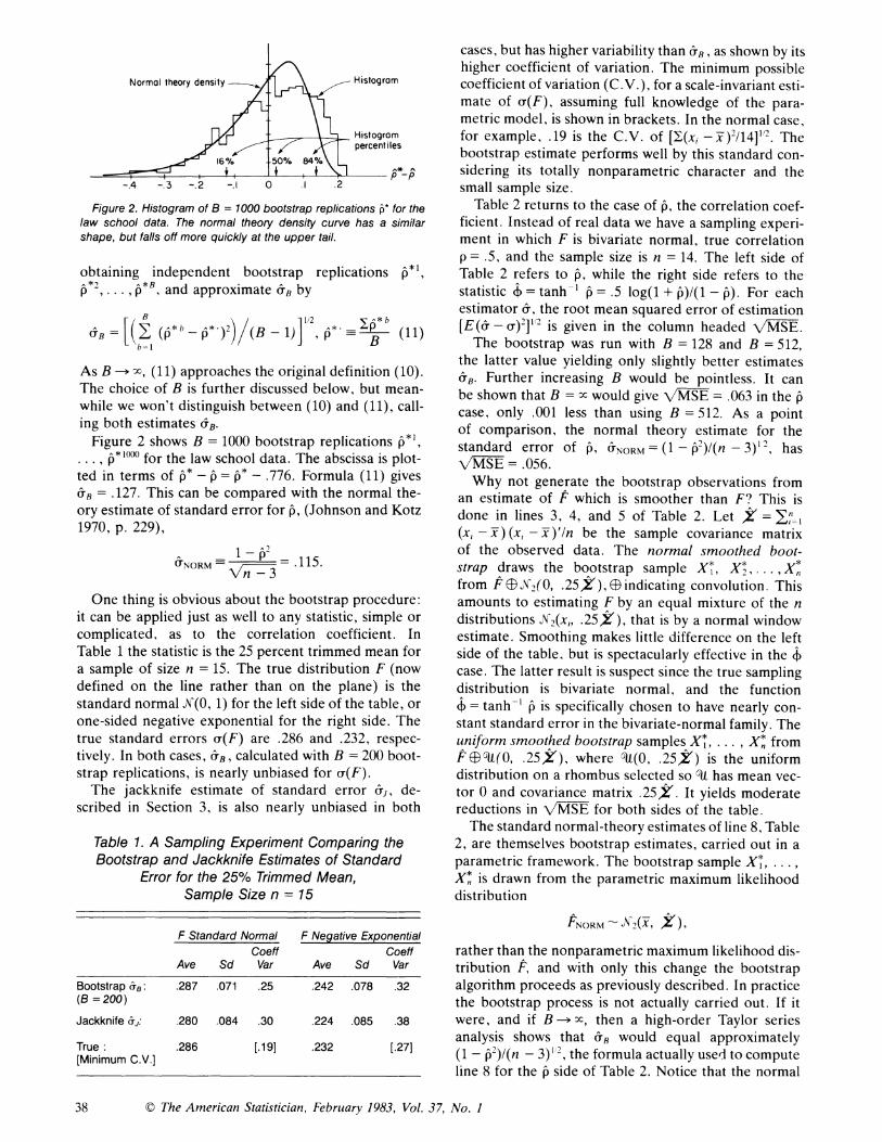
Figure 2. Histogram of B = 1000 bootstrap replications p* for the

law school data. The normal theory density curve has a similar

shape, but falls off more quickly at the upper tail.

obtaining independent bootstrap replications p', p*2 I p*B , and approximate&Bby

aB = [( E .-)p ) (B - 1) P_- (11)

As B xc, (11) approaches the original definition (10). The choice of B is further discussed below, but mean- while we won't distinguish between (10) and (11), call- ing both estimates 1B-

Figure 2 shows B = 1000 bootstrap replications p', . .., p*'? for the law school data. The abscissa is plot-

ted in terms of p* - p= p* - .776. Formula (11) gives aB = .127. This can be compared with the normal theory estimate of standard error for p, (Johnson and Kotz 1970, p. 229),

&NORM X z * 11 5 -

One thing is obvious about the bootstrap procedure: it can be applied just as well to any statistic, simple or complicated, as to the correlation coefficient. In Table 1 the statistic is the 25 percent trimmed mean for a sample of size n = 15. The true distribution F (now defined on the line rather than on the plane) is the standard normal X(0, 1) for the left side of the table, or one-sided negative exponential for the right side. The true standard errors a(F) are .286 and .232, respectively. In both cases, &B, calculated with B = 200 bootstrap replications, is nearly unbiased for ca(F).

The jackknife estimate of standard error &j, described in Section 3, is also nearly unbiased in both

Table 1. A Sampling Experiment Comparing the Bootstrap and Jackknife Estimates of Standard

Error for the 25% Trimmed Mean, Sample Size n = 15

F Standard Normal F Negative Exponential

Coeff Coeff Ave Sd Var Ave Sd Var

Bootstrap &B .287 .071 .25 .242 .078 .32 (B = 200)

Jackknife &JJ: .280 .084 .30 .224 .085 .38

True: .286 [.191 .232 [.27] [Minimum C.V.]

cases, but has higher variability than aB, as shown by its higher coefficient of variation. The minimum possible coefficient of variation (C.V.), for a scale-invariant estimate of a(F), assuming full knowledge of the parametric model, is shown in brackets. In the normal case, for example, .19 is the C.V. of [ I (x,--) /14]12. The bootstrap estimate performs well by this standard considering its totally nonparametric character and the small sample size.

Table 2 returns to the case of p, the correlation coefficient. Instead of real data we have a sampling experiment in which F is bivariate normal, true correlation p = .5, and the sample size is n = 14. The left side of Table 2 refers to p, while the right side refers to the statistic $ = tanhW -I = .5 log(1 + p)/(1 - p). For each estimator 6, the root mean squared error of estimation [E(a - U)2]1/2 is given in the column headed MSE.

The bootstrap was run with B = 128 and B = 512, the latter value yielding only slightly better estimates &B. Further increasing B would be pointless. It can be shown that B = x would give MSE = .063 in the p case, only .001 less than using B = 512. As a point of comparison, the normal theory estimate for the standard error of p, &NORM = (1 - )1(n - 3)12, has /MSE = .056.

Why not generate the bootstrap observations from an estimate of F which is smoother than F? This is done in lines 3, 4, and 5 of Table 2. Let X =, (x, - x-) (x, - x-)'In be the sample covariance matrix of the observed data. The normal smoothed bootstrap draws the bootstrap sample Xl, X*, .. ., X from F eD X2(O, .25Z), e indicating convolution. This amounts to estimating F by an equal mixture of the n distributions XNS(x,, .25k), that is by a normal window estimate. Smoothing makes little difference on the left side of the table, but is spectacularly effective in the 4 case. The latter result is suspect since the true sampling distribution is bivariate normal, and the function 4 = tanh-' p is specifically chosen to have nearly constant standard error in the bivariate-normal family. The uniform smoothed bootstrap samples X .,X* from Fe6DN0, .25,Z), where t(0, .25X) is the uniform distribution on a rhombus selected so t has mean vector 0 and covariance matrix .25,. It yields moderate reductions in MSE for both sides of the table.

The standard normal-theory estimates of line 8, Table 2, are themselves bootstrap estimates, carried out in a parametric framework. The bootstrap sample Xl, ... . X* is drawn from the parametric maximum likelihood distribution

F'NORM~ J<(,,)

rather than the nonparametric maximum likelihood distribution F, and with only this change the bootstrap algorithm proceeds as previously described. In practice the bootstrap process is not actually carried out. If it were, and if B-*x, then a high-order Taylor series analysis shows that UB would equal approximately (1 - ip2)/(n - 3)' 2 the formula actually used to compute line 8 for the p side of Table 2. Notice that the normal

38 ? The American Statistician, February 1983, Vol. 37, No. I

Table 2. Estimates of Standard Error for the Correlation Coefficient p and for + = tanh 1 p; Sample Size n = 14, Distribution F Bivariate Normal With True Correlation p = .5. From a Larger Table in Efron (1981b)

Summary Statistics for 200 Trials Standard Error Standard Error Estimates for p Estimates for )

Ave Std Dev CV VMSE Ave Std Dev CV VMSE

1. Bootstrap B= 128 .206 .066 .32 .067 .301 .065 .22 .065 2. Bootstrap B = 512 .206 .063 .31 .064 .301 .062 .21 .062 3. Normal Smoothed Bootstrap B 128 .200 .060 .30 .063 .296 .041 .14 .041 4. Uniform Smoothed Bootstrap B 128 .205 .061 .30 .062 .298 .058 .19 .058 5. Uniform Smoothed Bootstrap B 512 .205 .059 .29 .060 .296 .052 .18 .052

6. Jackknife .223 .085 .38 .085 .314 .090 .29 .091 7. Delta Method .175 .058 .33 .072 .244 .052 .21 .076

(Infinitesimal Jackknife)

8. Normal Theory .217 .056 .26 .056 .302 0 0 .003

True Standard Error .218 .299

smoothed bootstrap can be thought of as a compromise between using F and FNORM to begin the bootstrap process.

3. THE JACKKNIFE

The jackknife estimate of standard error was introduced by Tukey in 1958 (see Miller 1974). Let P(i) = P(xI, x2, . . ., xi-1, xi+1, . . ., x,) be the value of the statistic when xi is deleted from the data set, and let P(.)= (1/n) In P(i). The jackknife formula is

- ) n) 1/2 UJ= [((n - 1)/n ) (^ p(.)_ t))2]'

Like the bootstrap, the jackknife can be applied to any statistic that is a function of n independent and identically distributed variables. It performs less well than the bootstrap in Tables 1 and 2, and in most cases investi- gated by the author (see Efron 1982), but requires less computation. In fact the two methods are closely related, which we shall now show.

Suppose the statistic of interest, which we will now call O(xl, X2, . . . , Xv) is of functional form: 0 F0(), where 0(F) is a functional assigning a real number to any distribution F on the sample space. Both examples in Section 2 are of this form. Let P= (P1, P2, . PO) be a probability vector having nonnegative weights sum- ming to one, and define the reweighted empirical distribution F(P): mass Pi on xi, i = 1, 2, . . ., n. Correspond- ing to P is a resampled value of the statistic of interest, say 0(P) = 0(F(P)). The shorthand notation 0(P) as- sumes that the data points x1, x2, ..., xn are fixed at their observed values.

Another way to describe the bootstrap estimate 6B iS as follows. Let P* indicate a vector drawn from the rescaled multinomial distribution

P* 4ultn(n, P?)ln, (Po (1/n) (1, 1, . 1)'), (12)

meaning the observed proportions from n random draws on n categories, with equal probability 1/n for each category. Then

0B [var*, (p*)]/2, (13)

where var, indicates variance under distribution (12). (This is true because we can take P* = #fX* = xi}ln in step 2 of the bootstrap algorithm.)

Figure 3 illustrates the situation for the case n = 3. There are 10 possible bootstrap points. For example, the point P* = (2, 3, 0)' is the second dot from the left on the lower side of the triangle, and occurs with bootstrap probability 9, under (12). It indicates a bootstrap sample Xl, X", X3 consisting of two x,'s and one x2. The center point Po (3, 3, 3)' has bootstrap probability 9.

The jackknife resamples the statistic at the n points

P(i) (1/(n - 1)) (1, 1, . . . 0 1,, 1, I . ., 1)' (O in ith place),

i = 1, 2, ..., n. These are indicated by the open circles in Figure 3. In general there are n jackknife points, compared with (2n7 1) bootstrap points.

The trouble with bootstrap formula (13) is that 0(P) is usually a complicated function of P (think of the examples in Sec. 2), and so var, 0(P*) cannot be evalu-

x3

1/27

1/9 1/9

p (2) P 0 (1)

1/9 2/9 1/9

x1 1/27 1/9 P (3) 1/9 1/27 x2

Figure 3. The bootstrap and jackknife sampling points in the case n = 3. The bootstrap points (-) are shown with their probabilities.

(? The American Statistician, February 1983, Vol. 37, No. 1 39

ated except by Monte Carlo methods. The jackknife trick approximates 0(P) by a linear function of P, say 0L (P). and then uses the known covariance structure of (12) to evaluate var, OL(P*). The approximator OL(P) is chosen to match 0(P) at the n points P= P(,). It is not hard to see that

OL(P) = 0(.) + (P P0)YU (14)

where 0(.)= (1/n) L; 0(,1=/(in) E) 0(P(,)), and U is a column vector with coordinates U, = (n - 1) (O(.) - 6(,).

Theorem. The jackknife estimate of standard error equals

crJ=Kn _i var. OL(P*)

which is [nl(n -1)]1 2times the bootstrap estimate of standard error for 0L (Efron 1982).

In other words the jackknife is, almost,' a bootstrap itself. The advantage of working with 0L rather than 0 is that there is no need for Monte Carlo: var* OL(P*) =var, (P* - P0)'U =- IU>ln, using the covariance matrix for (12) and the fact that )2U, = 0. The disadvantage is (usually) increased error of estimation, as seen in Tables 1 and 2.

The fact that &j is almost 0&B for a linear approximation of 0 does not mean that &j is a reasonable approximation for the actual 6B. That depends on how well 0L approximates 0. In the case where 0 is the sample median, for instance, the approximation is very poor.

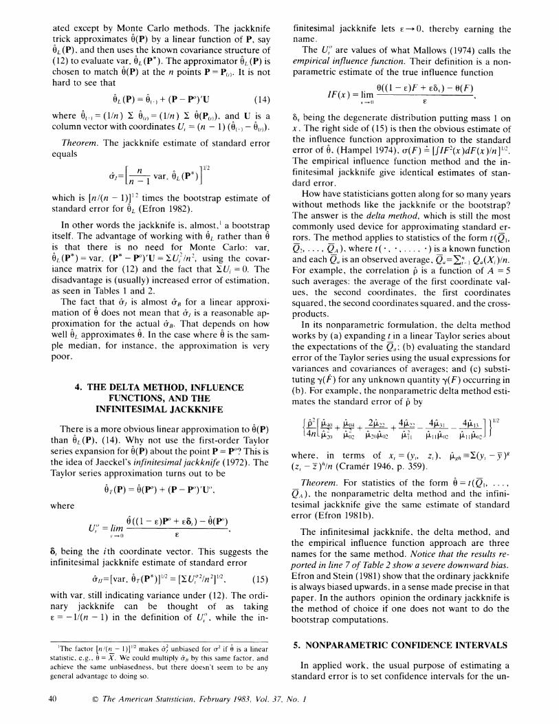
4. THE DELTA METHOD, INFLUENCE FUNCTIONS, AND THE

INFINITESIMAL JACKKNIFE

There is a more obvious linear approximation to 0(P) than OL(P), (14). Why not use the first-order Taylor series expansion for 0(P) about the point P - P0? This is the idea of Jaeckel's infinitesimal jackknife (1972). The Taylor series approximation turns out to be

OT(P) = 0(PO) + (P -P'U',

where

,lim 6 ((1 - E)P0 + Es,) - 0(P0) F - (0 F

5, being the ith coordinate vector. This suggests the infinitesimal jackknife estimate of standard error

&SsJ= [var. 6T(P*)]'/ = [iuo 2In ] 112 ( 15) with var. still indicating variance under (12). The ordinary jackknife can be thought of as taking E = -1/(n - 1) in the definition of U.'. while the in-

finitesimal jackknife lets E-+ 0, thereby earning the name.

The U,7 are values of what Mallows (1974) calls the empirical influence function. Their definition is a nonparametric estimate of the true influence function

IF(x) = lim 0((1 - F)F + Eb,) - 0(F) lF( ) = )

ll e (} ~~~E

6. being the degenerate distribution putting mass 1 on x. The right side of (15) is then the obvious estimate of the influence function approximation to the standard error of 0, (Hampel 1974), u(F) [fIF(x)dF(x)In]'. The empirical influence function method and the infinitesimal jackknife give identical estimates of standard error.

How have statisticians gotten along for so many years without methods like the jackknife or the bootstrap? The answer is the delta method, which is still the most commonly used device for approximating standard errors. The method applies to statistics of the form t(Q1, Q2. QA) where t(,.. ) is a known function and each QO is an observed average, QOa= >% I Qa (Xi)/n. For example, the correlation p is a function of A = 5 such averages: the average of the first coordinate values, the second coordinates, the first coordinates squared, the second coordinates squared, and the cross- products.

In its nonparametric formulation, the delta method works by (a) expanding t in a linear Taylor series about the expectations of the Qa; (b) evaluating the standard error of the Taylor series using the usual expressions for variances and covariances of averages; and (c) substi- tuting y(F) for any unknown quantity -y(F) occurring in (b). For example, the nonparametric delta method estimates the standard error of p by

J 0+ 11iO + 4 422 4i31 4 13112

l4nLp.20 P,02 P2(Jf)2 PI PI!Pu(-2 IP1 P(J2 JJ

where, in terms of x, (y,, z,), 14J2- - Y )

(z, - z)"ln (Cramer 1946, p. 359).

Theorem. For statistics of the form 0 t(Q.. QA ) the nonparametric delta method and the infinitesimal jackknife give the same estimate of standard error (Efron 1981b).

The infinitesimal jackknife, the delta method, and the empirical influence function approach are three names for the same method. Notice that the results re- ported in line 7 of Table 2 show a severe downward bias. Efron and Stein (1981) show that the ordinary jackknife is always biased upwards, in a sense made precise in that paper. In the authors opinion the ordinary jackknife is the method of choice if one does not want to do the bootstrap computations.

5. NONPARAMETRIC CONFIDENCE INTERVALS

In applied work, the usual purpose of estimating a standard error is to set confidence intervals for the un-

'The factor [nl(n - 1)11/2 makes 6&' unbiased for a& if 0 is a linear statistic, e.g.. 0 = X. We could multiplv a,, by this same factor, and achieve the same unbiasedness. but there doesn't seem to be any general advantage to doing so.

40 (? The American Statistician. February 1983, Vol. 37, No. I

known paramater. These are typically of the crude form o + z,,,cr, with zat being the 100(1 - a) percentile point of a standard normal distribution. We can, and do, use the bootstrap and jackknife estimates 'B, ( in this way. However in small-sample parametric situations, where we can do exact calculations, confidence intervals are often highly asymmetric about the best point estimate 0. This asymmetry, which is 0(1//'>) in magnitude, is substantially more important than the Student's t correction (replacing 0 ? Z,, by 0 + t<,, with t, the 100(1 - a) percentile point of the appropriate t distribution), which is only O(1/n). This section discusses some nonparametric methods of assigning confidence intervals, which attempt to capture the correct asymmetry. it is abbreviated from a longer discussion in Efron (1981c), and also Chapter 10 of Efron (1982). All of this work is highly speculative, though encouraging.

We return to the law school example of Section 2. Suppose for the moment that we believe the data come from a bivariate normal distribution. The standard 68 percent central confidence interval (i.e., x= .16, 1 - 2a = .68) for p in this case is [.62, .87] = - .16, p + .09], obtained by inverting the approximation 4) N(4) + pI(2(n - 1)), 1/(n - 3)). Compared to the crude interval '

? Z.16 cTNORM = Z = [- .12, p + .12], this demonstrates the magnitude of the asymmetry effect described previously.

The asymmetry of the confidence interval [p-.16, p + .09] relates to the asymmetry of the normal-theory density curve for p5, as shown in Figure 2. The bootstrap histogram shows this same asymmetry. The striking similarity between the histogram and the density curve suggests that we can use the bootstrap results more ambitiously than simply to compute &B.

Two ways of forming nonparametric confidence intervals from the bootstrap histogram are discussed in Ef- ron (1981c). The first, called the percentile method, uses the lOOa and 100(1 - a) percentiles of the bootstrap histogram, say

OE[O(t), O(1 - t)], (16)

as a putative 1 - 2a central confidence interval for the unknown parameter 0. Letting

#I-) _ b < t}

then 0(a) = (a), 0(1-()='(1 - a). In the law school example, with B = 1000 and t - .16, the 68 percent interval is p E [.65, .91] = [p - .12, p + .13], almost exactly the same as the crude normal-theory interval P C+ NORM

Notice that the median of the bootstrap histogram is substantially higher than p in Figure 2. In fact, CO5) = .433, only 433 out of 1000 bootstrap replications having p* <f. The bias-corrected percentile method makes an adjustment for this type of bias. Let ?(z) indicate the CDF of the standard normal distribution, so 1>(za) = 1 - ax, and define

The bias-corrected putative 1 - 2(x central confidence interval is defined to be

0 E [ -{)(2zo - zX)}, C 1{1(2zo + z,)}]. (17)

If C(O) = .50, the median unbiased case, then z0 = 0 and (8) reduce to the uncorrected percentile interval (16). Otherwise the results can be quite different. In the law school example z0 = .F(.433) = - .17, and for a = .16, (8) gives pE[C'1{f(-1.34)}, C-&{sF(.66)}] =

-.17, p + .10]. This agrees nicely with the normal- theory interval [A - .16, p + .09].

Table 3 shows the results of a small sampling experiment, only 10 trials, in which the true distribution Fwas bivariate normal, p = .5. The bias-corrected percentile method shows impressive agreement with the normal- theory intervals. Even better are the smoothed intervals, last column. Here the bootstrap replications were obtained by sampling from tfflDX(O, .25X), as in line 3 of Table 2, and then applying (17) to the resulting histogram.

There are some theoretical arguments supporting (16) and (17). If there exists a normalizing transformation, in the same sense as = tanh- 1p is normalizing for the correlation coefficient under bivariate-normal sampling, then the bias-corrected percentile method au- tomatically produces the appropriate confidence intervals. This is interesting since we do not have to know the form of the normalizing transformation to apply (17). Bayesian and frequentist justifications are given also in Efron (1981c). None of these arguments is overwhelm- ing, and in fact (17) and (16) sometimes perform poor- ly. Some other methods are suggested in Efron (1981c), but the appropriate theory is still far from clear.

6. BIAS ESTIMATION

Quenouille (1949) originally introduced the jackknife as a nonparametric device for estimating bias. Let us denote the bias of a functional statistic 0 = 0(s) by

Table 3. Central 68% Confidence Intervals for p, 10 Trials of Xi, X2, ..., X1,5 Bivariate Normal With True

p=.5. Each Interval Has p Subtracted From Both Endpoints

Smoothed and Bias-Corrected Bias-Corrected

Normal Percentile Percentile Percentile Trial p Theory Method Method Method

1 .16 (-.29, .26) (-.29, .24) (-.28, .25) (-.28, .24) 2 .75 (-.17, .09) (-.05, .08) (-.13, .04) (-.12, .08) 3 .55 (-.25, .16) (-.24, .16) (-.34, .12) (-.27, .15) 4 .53 (-.26, .17) (-.16, .16) (-.19, .13) (-.21, .16) 5 .73 (-.18, .10) (-.12, .14) (-.16, .10) (-.20, .10) 6 .50 (-.26, .18) (-.18, .18) (-.22, .15) (-.26, .14) 7 .70 (-.20, .11) (-.17, .12) (-.21, .10) (-.18, .11) 8 .30 (-.29, .23) (-.29, .25) (-.33, .24) (- .29, .25) 9 .33 (-.29, .22) (-.36, .24) (-.30, .27) (-.30, .26) 1 0 .22 (- .29, .24) (- .50, .34) (- .48, .36) (-.38, .34)

AVE .48 (-.25, .18) (-.21, .19) (-.26, .18) (-.25, .18)


1, a = E{0(F) - O(F)}. In the notation of Section 3, Quenouille's estimate is

pi= (n - 1)(0() -) (18) Subtracting 1j from 0, to correct the bias leads to the jackknife estimate of 0, 0;= nO - (n - 1)0(.), see Miller (1974), and also Schucany, Gray, and Owen (1971). There are many ways to justify (18). Here we follow

the same line of argument as in the justification of 6f]. The bootstrap estimate of 1, which has an obvious mo- tivation, is introduced, and then (18) is related to the bootstrap estimate by a Taylor series argument.

The bias can be thought of as a function of the unknown probability distribution F, 1 = 1(F). The bootstrap estimate of bias is simply

B = 1(F) = E4f0(F*) - 0(F)}. (19)

Here E* indicates expectation with respect to bootstrap sampling, and Ft* is the empirical distribution of the bootstrap sample.

In practice 1B must be approximated by Monte Carlo methods. The only change in the algorithm described in Section 2 is at step (iii), when instead of (or in addition to) CB we calculate

B

In the sampling experiment of Table 2 the true bias, of pj for estimating p, is 13 = -.014. The bootstrap estimate 1B, taking B = 128, has expectation -.014 and standard deviation .031 in this case, while 1J has expectation -.017, standard deviation .040. Bias is a negligible source of statistical error in this situation compared with variability. In applications this is usually made clear by comparison of 1B with CB.

The estimates (18) and (19) are closely related to each other. The argument is the same as in Section 3, except that we approximate 0(P) with a quadratic rather than a linear function of P, say OQ (P) =

+(P- PO)'b + 1(P - PO)'c(P- PO). Let OQ(P) be any such quadratic satisfying

OQ(PO) = o(Po) = 0 and OQ(P(i)) = 0(P(o)), i = 1, 2, .. ., n.

Theorem. The jackknife estimate of bias equals

n-in J=n - 1 [E{Q (P*) - '}],

which is nl(n - 1) times the bootstrap estimate of bias for OQ (Efron 1982).

Once again, the jackknife is, almost, a bootstrap estimate itself, except applied to a convenient approximation of 0(P).

More general problems. There is nothing special about bias and standard error as far as the bootstrap is concerned. The bootstrap procedure can be applied to almost any estimation problem.

Suppose that R (X,, X2, . .., Xn; F) is a random variable, and we are interested in estimating some aspect of R 's distribution. (So far we have taken R = 0(F) - 0(F)

and have been interested in the expectation , and the standard deviation cr of R.) The bootstrap algorithm proceeds as described in Section 2, with these two changes: at step (ii), we calculate the bootstrap replication R * = R (X*, X*, ..., X*; F), and at step (iii) we calculate the distributional property of interest from the empirical distribution of the bootstrap replications R* 1

D* 2 D* B R , . . . , R

For example, we might be interested in the probability that the usual t statistic VNi (X - ,u)/S exceeds 2, where ,u = E{X} and S2 = I(Xi - X)21(n - 1). Then R =NV"(X* - -)/S*, and the bootstrap estimate is #fR*b>2}1B. This calculation is used in Section 9 of Efron (1981c) to get confidence intervals for the mean ,u in a situation where iiormality is suspect.

The cross-validation problem of Sections 8 and 9 involves a different type of error random variable R. It will be useful there to use a jackknife-type approximation to the bootstrap expectation of R,

E*{R* } = R? + (n - 1)(R(.) - R?). (20)

Here R 0 = R (xi, x2, . . ., Xn; F) and R(.) = (ll/n )R(i), R(i) = R (xi, x2, . . . , xi 1, xi+1, . . ., Xn; F). The justification of (20) is the same as for the theorem of this section, being based on a quadratic approximation formula.

7. MORE COMPLICATED DATA SETS

So far we have considered the simplest kind of data sets, where all the observations come from the same distribution F. The bootstrap idea, and jackknife-type approximations (which are not discussed here), can be applied to much more complicated situations. We begin with a two-sample problem.

The data in our first example consist of two independent random samples,

Xli X2, . . . X X. - F and YI, Y2i ... ., Yn~ -C,

F and G being two possibly different distributions on the real line. The statistic of interest is the Hodges- Lehmann shift estimate

0=median{yj-x;i=1, ..., m,j=1, ..., n}.

We desire an estimate of the standard error c(F, G). The bootstrap estimate is simply

UBO(F, 6),

6 being the empirical distribution of the yi. This is evaluated by Monte Carlo, as in Section 3, with obvious modifications: a bootstrap sample now consists of a random sample X*, X*, ..., X, drawn from F and an independent random sample Y*, ..., Y* drawn from . (In other words, m draws with replacement from {x1,

X2 . .,m}, and n draws with replacement from {Yf, Y2, ***mYn}-) The bootstrap replication 0* is the median of

the mn differences yj* - Xi*. Then UB iS approximated from B independent such replications as on the right side of (11).

Table 4 shows the results of a sampling experiment in

42 ?) The American Statistician, February 1983, Vol. 37, No. I

Table 4. Bootstrap Estimates of Standard Error for the Hodges-Lehmann Two-Sample Shift Estimate; m = 6, n = 9; True Distributions Both F and G

Uniform [0, 1]

Expectation St. Dev. C. V. MSE

B = 100 .165 .030 .18 .030 Separate

B = 200 .166 .031 .19 .031

B = 100 .145 .028 .19 .036 Combined

B = 200 .149 .025 .17 .031

True Standard Error .167

which m = 6, n = 9, and both F and G were uniform distributions on the interval [0, 1]. The table is based on 100 trials of the situation. The true standard error is c(F, G) = .167. "Separate" refers to UB calculated exactly as described in the previous paragraph. The improvement in going from B = 100 to B = 200 is too small to show up in the table.

"Combined" refers to the following idea: suppose we believe that G is really a translate of F. Then it wastes information to estimate F and G separately. Instead we can form the combined empirical distribution

I 1 H: mass m+ on m + n

X1, X2, . . ., Xm, Yi - 6, Y2 - 0. yYn-6.

All m + n bootstrap variates Xl, ..., XA, Y7, ,.Yn are then sampled independently from H. (We could add 0 back to the Y, values, but this has no effect on the bootstrap standard error estimate, since it just adds the constant 0 to each bootstrap replication V*.)

The combined method gives no improvement here, but it might be valuable in a many-sample problem where there are small numbers of observations in each sample, a situation that arises in stratified sampling. (See Efron 1982, Ch. 8.) The main point here is that "bootstrap" is not a well-defined verb, and that there may be more than one way to proceed in complicated situations. Next we consider regression problems, where again there is a choice of bootstrapping methods.

In a typical regression problem we observe n independent real-valued quantitives Yi =yi,

Y, =gi(I) + Ei, i = 1, 2, . . , n. (21)

The functions g,( ) are of known form, usually gi() = g(3; ti), where ti is an observed p-dimensional vector of covariates; i is a vector of unknown parameters we wish to estimate. The gi are an independent and identically distributed random sample from some distribution F on the real line,

81 E 2 . . En , F

where F is assumed to be centered at zero in some sense, perhaps E{E} =0 or Prob{e < 0} =0.5.

Having observed the data vector V = y =(y1., n we estimate <3 by minimizing some measure of distance

between y and the vector of predicted values q(3)= (gl (13),. gn (13)),

:min D(y, iq(1)).

The most common choice of D is D (y, q) =

(yi - i)

Having calculated 1, we can modify the one-sample bootstrap algorithm of Section 2, and obtain an estimate of 13's variability:

(i) Construct F putting mass l/n at each observed residual,

F: mass l/n on ii = y, - g, (13)

(ii) Construct a bootstrap data set

Y7 = g() + E*, i = 1, 2, n,

where the E* are drawn independently from F, and calculate

*:min D (Y*, M(n))

(iii) Do step (ii) some large number B of times, obtaining independent bootstrap replications *1, *2 .. *B, and estimate the covariance matrix of (3 by

[E (0*b - *) (0*- 3*.) ) (B - 1)1,

(13* = 143*b)

In ordinary linear regression we have gi(1) = t' 1 and D(y, lj) = I(yi - qi)2. Section 7 of Efron (1979a) shows that in this case the algorithm above can be carried out theoretically, B =, and yields

n it (B= (> tit;) 6.2 = E I/n. (22)

This is the usual answer, except for dividing by n instead of n - p in &2. Of course the advantage of the bootstrap approach is that XB can just as well be calculated if, say, gi(1) = exp (ti 1) and D(y, 1q) = [|, - 'rij

There is another simpler way to bootstrap the regression problem. We can consider each covariate- response pair x, = (t,, yi) to be a single data point obtained by random sampling from a distribution F on p + 1 dimension space. Then we apply the one-sample bootstrap of Section 2 to the data set xi, x,, ..., xn.

The two bootstrap methods for the regression problem are asymptotically equivalent, but can perform quite differently in small-sample situations. The simple method, described last, takes less advantage of the special structure of the regression problem. It does not give answer (22) in the case of ordinary least squares. On the other hand thle simple method gives a trustworthy estimate of 1's variability even if the regression model (21) is not correct. For this reason we use the simple method of bootstrapping on the error rate prediction problem of Sections 9 and 10.

As a final example of bootstrapping complicated data

?) The American Statistician, February 1983, Vol. 37, No. 1 43

we consider a two-sample problem with censored data. The data are the leukemia remission times listed in Table 1 of Cox (1972). The sample sizes are m = n = 21. Treatment-group remission times (weeks) are 6+, 6, 6, 6, 7 9+ 10 +, 10, 11+, 13, 16, 17+, 19+, 20+, 22, 23, 25+, 32+, 32+, 34+, 35+; control-group remission times (weeks) are 1. 1, 2, 2, 3, 4, 4, 5, 5, 8, 8, 8, 8, 11, 11, 12. 12, 15, 17, 22, 23. Here 6+ indicates a censored remission time, known only to exceed 6 weeks, while 6 is an uncensored remission time of exactly 6 weeks. None of the control-group times were censored.

We assume Cox's proportional hazards model, the hazard rate in the control group equaling eO times that in the Treatment group. The partial likelihood estimate of 3 is 3 = 1.51, and we want to estimate the standard error of 3. (Cox gets 1.65, not 1.51. Here we are using Breslow's convention for ties (1972), which accounts for the discrepancy.)

Figure 4 shows the histogram for 1000 bootstrap replications of *. Each replication was obtained by the two-sample method described for the Hodges-Lehmann estimate:

(i) Construct FPputting mass at each point 6+, 6, 6, 35+, and 6 putting mass Iy at each point 1, 1, . . .

23. (Notice that the "points' in F include the censoring information.)

(ii) Draw Xl, X*, . . .<, X* by random sampling from F, and likewise YL Y,, ..., Y*, by random sampling from G. Calculate * by applying the partial-likelihood method to the bootstrap data.

The bootstrap estimate of standard error for 3, as given by (11), is &B = .42. This agrees nicely with Cox's asymptotic estimate 6^ = .41. However, the percentile method gives quite different confidence intervals from those obtained by the usual method. For x = .05, 1 - 2(x = .90, the latter interval is 1.51 + 1.65 - .41 = [.83. 2.19]. The percentile method gives the 90 percent central interval [.98, 2.35]. Notice that (2.35 - 1.51)! (1.51 - .98) = 1.58, so that the percentile interval is considerably larger to the right of 3 than to the left. (The bias-corrected percentile method gives almost the same answers as the uncorrected method in this case since C((r) = .49.)

0 5 1.0 1.5 2.0 2.5 3.0

Figure 4. Histogram of 1000 bootstrap replications of * for the leukemia data, proportional hazards model. Courtesy of Rob Tibshirani, Stanford.

There are other reasonable ways to bootstrap censored data. One of these is described in Efron (1981a), which also contains a theoretical justification for the method used to construct Figure 4.

8. CROSS-VALIDATION

Cross-validation is an old but useful idea, whose time seems to have come again with the advent of modern computers. We discuss it in the context of estimating the error rate of a prediction rule. (There are other important uses; see Stone 1974; Geisser 1975.)

The prediction problem is as follows: each data point xI = (t,, y,) consists of a p-dimensional vector of explanatory variables t,, and a response variable y,. Here we assume y, can take on only two possible values, say 0 or 1, indicating two possible responses, live or dead, male or female, success or failure, and so on. We observe xi, xi, . . ., xn, called collectively the training set, and indicated x = (xi, x2, . . ., xn). We have in mind a formula -r(t; x) for constructing a prediction rule from the training set, also taking on values either 0 or 1. Given a new explanatory vector t0,, the value -r(to; x) is supposed to predict the corresponding response y(.

We assume that each x, is an independent realization of X = (T, Y), a random vector having some distribution F on p + 1-dimensional space, and likewise for the "new case" X(, = (T(, Y(). The true error rate err of the prediction rule -q(; x) is the expected probability of error over X( - F with x fixed,

err=E{Q[Yn, -r(T(, x)]}.

where Q [y, -r] is the error indicator

Q[Y' N]= 1 if y , -q. An obvious estimate of err is the apparent error rate

~~~~~~~~~~~~1 1 err=- E{Q [Y(,, -(T(X; x)]} n Q [y, ,-(t,; x)]

The symbol E indicates expectation with respect to the empirical distribution F, putting mass 1/n on each x,. The apparent error rate is likely to underestimate the true error rate, since we are evaluating -r(, x)'s per- formance on the same set of data used in its construction. A random variable of interest is the overoptimism, true minus apparent error rate,

R (x, F) = err - err

= E{Q [ Y(,, q(T1; x)]} - E{Q [ Y(, -(TO; x)]}. (23)

The expectation of R (X, F) over the random choice of XI, X9,, Xn from F,

w(F) ER (X, F) (24) is the expected overoptimism.

The cross-validated estimate of err is

err' Z Q [y, -j(t,; X())] .

-r(t,; x, ) being the prediction rule based on x(,) =

44 ? The American Statistician, February 1983, Vol. 37, No. I

(xl, x,, ... . x,i-, x?+l, ... I, x). In other words err. is the error rate over the observed data set, not allowing xI = (t,, y,) to enter into the construction of the rule for its own prediction. It is intuitively obvious that err' is a less biased estimator of err than is err. In what follows we consider how well err' estimates err, or equivalently how well

w -err' - err

estimates R (x, F) = err - err. (These are equivalent problems since err' - err = w - R(x, F).) We have used the notation , rather than R., because it turns out later that it is actually w being estimated.

We consider a sampling experiment involving Fish- er's linear discriminant function. The dimension is p = 2 and the sample size of the training set is n = 14. The distribution F is as follows: Y = 0 or 1 with probability -, and given Y = y the predictor vector T is bivariate normal with identity covariance matrix and mean vector (y - I, 0). If F were known to the statistician, the ideal prediction rule would be to guess yo = 0 if the first component of t(, was '0, and to guess y( = 1 otherwise. Since F is assumed unknown, we must estimate a prediction rule from the training set.

We use the prediction rule based on Fisher's estimated linear discriminant function (Efron 1975),

-rj(t; x) 1if x + t is>

The quantities & and a are defined in terms of n, and nl, the number of y, equal to zero and one, respectively; to and tl, the averages of the t, corresponding to those yi equaling zero and one, respectively; and S=

tit' - n(tnt() - nittljl/n:

(X [t 1S -1t- tl tS -t,]l2,

13 = [tS - t 5 l

Table 5 shows the results of 10 simulations ("trials") of this situation. The expected overoptimism, obtained from 100 trials, is w = .098, so that R = err - err is typically quite large. However, R is also quite variable from

Table 5. The First 10 Trials of a Sampling Experiment Involving Fisher's Linear Discriminant Function. The

Training Set Has Size n = 14. The Expected Overoptimism is w =.096, see Table 6

Error Rates Estimates of Overoptimism Appar- Over- Cross- Jack- Bootstrap

True ent optimism validation knife (B = 200) Trial n., n, err err R wt

A B

1 9,5 .45a .286 .172 .214 .214 .083 2 6,8 .312 .357 -.045 .000 .066 .098 3 7,7 .313 .357 -.044 .071 .066 .110 4 8,6 .351 .429 -.078 .071 .066 .107 5 8,6 .330 .357 - .027, .143 .148 .1 02 6 8,6 .318 .143 .175 .214 .194 .073 7 8,6 .310 .071 .239 .071 .066 .087 8 6,8 .382 .286 .094 .071 .056 .097 9 7,7 .360 .429 -.069 .071 .087 . 127

10 8,6 .335 .143 - .192 .000 .010 .048

trial to trial, often being negative. The cross-validation estimate w is positive in all 10 cases, and does not correlate with R. This relates to the comment that wx is trying to estimate w rather than R. We will see later that w. has expectation .091, and so is nearly unbiased for w. However, w is too variable itself to be very useful for estimating R, which is to say that err' is not a particularly good estimate of err. These points are discussed further in Section 9, where the two other estimates of w appearing in Table 5, C(j and CO, are introduced.

9. BOOTSTRAP AND JACKKNIFE ESTIMATES FOR THE PREDICTION PROBLEMS

At the end of Section 6 we described a method for applying the boostrap to any random variable R (X, F). Now we use that method on the overoptimism random variable (23), and obtain a bootstrap estimate of the expected overoptimism w(F).

The bootstrap estimate of w w(F), (24), is simply

COB = W(I(F).

As usual (aB must be approximated by Monte Carlo. We generate independent bootstrap replications R* 1, R,

R* B, and take

l 1B WB ==- R b

B h=1

As B goes to infinity this last expression approaches E*{R* }, the expectation of R* under bootstrap resampling, which is by definition the same quantity as W(() = CB. The bootstrap estimates CB seen in the last column of Table 5 are considerably less variable than the cross-validation estimates X .

What does a typical bootstrap replication consist of in this situation? As in Section 3 let P* = (P*, P*, . . ., P* ) indicate the bootstrap resampling proportions P* = #{X, = x,}ln. (Notice that we are considering each vector x, = (t,, y,) as a single sample point for the purpose of carrying out the bootstrap algorithm.) Fol- lowing through definition (13), it is not hard to see that

n

R* =R(X*, F)= (P -P*) Q[yI, -r(t,; X*)], (25)

where P?= (1, 1, . 1)'/n as before, and -(, X*) is the prediction rule based on the bootstrap sample.

Table 6 shows the results of two simulation experiments (100 trials each) involving Fisher's linear discriminant fraction. The left side relates to the bivariate normal situation described in Section 8: sample size n = 14. dimension d = 2, mean vectors for the two randomly selected normal distributions = (+,, 0). The right side still has n = 14, but the dimension has been raised to 5, with mean vectors (+1, 0, 0, 0, 0). Fuller descriptions appear in Chapter 7 of Efron (1982).

Seven estimates of overoptimism were considered. In the d = 2 situation, the cross-validation estimate ~, for example, had expectation .091, standard deviation .073, and correlation - .07 with R. This gave root mean


Table 6. Two Sampling Experiments Involving Fisher's Linear Discriminant Function. The Left Side of the Table Relates to the Situation of Table 5: n = 14, d = 2, True Mean Vectors = (-+-2, 0).

The Right Side Relates to n = 14, d = 5, True Mean Vectors = (1 0, 0, 0, 0)

Dimension 2 Dimension 5 Overoptimism Exp. Sd. Exp. Sd.

R(X, F) w = .096 .113 Corr MSE w =. 184 .099 Corr. VM/ISE

1. Ideal Constant .096 0 0 .113 .184 0 0 .099 2. Cross-

Validation .091 .073 -.07 .139 .170 .094 -.15 .147 3. Jackknife .093 .068 -.23 .145 .167 .089 -.26 .150 4. Bootstrap

(B = 200) .080 .028 -.64 .135 .103 .031 -.58 .145 5. BootRand

(B = 200) .087 .026 -.55 .130 .147 .020 -.31 .114 6. BootAve

(B = 200) .100 .036 -.18 .125 .172 .041 -.25 .118 7. Zero 0 0 0 .149 0 0 0 .209

squared error, of w for estimating R or equivalently of err, for estimating err,

[E[(w - RI 2 [E(err- - err) -] .139.

The bootstrap, line 4, did only slightly better, 'M S-E= .135. The zero estimate C -= 0, line 7, had MSE= .149,

which is also [E(err - err)2], the MSE of estimating err by the apparent error err, with zero correction for overoptimism. The "ideal constant" is w itself. If we knew w, which we don't in genuine applications, we would use the bias-corrected estimate err + w. Line 1, left side, says that this ideal correction gives

'MS-E = .113. We see that neither cross-validation nor the bootstrap

are much of an improvement over making no correction at all, though the situation is more favorable on the right side of Table 6. Estimators 5 and 6, which will be described later, perform noticeably better.

The "jackknife," line 3, refers to the following idea: since CB = E*{R*} is a bootstrap expectation, we can approximate that expectation by (19). In this case (25) gives R" = 0, so the jackknife approximation is simply cji= (n - 1) R(.). Evaluating this last expression, as in Chapter 7 of Efron (1982), gives

w n { Q[y,, q(t,, X(,)) - Q[y, q(t,, X(i))]) n}

This looks very much like the cross-validation estimate, which can be written

n

w IQ nE{[Y" 1l(t,, x(,)] Q[y,, 9(t,, x)]}.

As a matter of fact, C(i and w have asymptotic correlation one (Gong 1982). Their nearly perfect correlation can be seen in Table 5. In the sampling experiments of Table 6, corr(Uj, UT) =.93 on the left side, and .98 on the right side. The point here is that the cross- validation estimate &1) is, essentially, a Taylor series approximation to the bootstrap estimate c%.

Even though COB and wX are closely related in theory and are asymptotically equivalent, they behave very differently in Table 6: wX is nearly unbiased and un- correlated with R, but has enormous variability; COB has small variability, but is biased downwards, particularly in the right-hand case, and highly negatively correlated with R. The poor performances of the two estimators are due to different causes, and there are some grounds of hope for a favorable hybrid.

"BootRand," line 5, modified the bootstrap estimate in just one way: instead of drawing the bootstrap sample Xl*, X*. X* from F, it was drawn from

FRAND: mass ((1 - )In on (t,, 1)

i =l1, 2, .. ., n.

This is a distribution supported on 2n points, the observed points x, = (t,, y,) and also the complementary points (t,, 1 - y,). The probabilities rr, were those natu- rally associated with the linear discriminant function,

rr, 1/1 +exp - ((x + t' )]

(see Efron 1975), except that rr, was always forced to lie in the interval [.1, .91.

Drawing the bootstrap sample X*. X* from FRAND instead of Fis a form of smoothing, not unlike the smoothed bootstraps of Section 2. In both cases we support the estimate of F on points beyond those actually observed in the sample. Here the smoothing is en- tirely in the response variable y. In complicated problems, such as the one described in Section 10, t, can have complex structure (censoring, missing values, cardinal and ordinal scales, discrete and continuous variates, etc.) making it difficult to smooth in the t space. Notice that in Table 6 BootRand is an improvement over the ordinary bootstrap in every way: it has smaller bias, smaller standard deviation, and smaller negative correlation with R. The decrease in MSE is especially impressive on the right side of the table.

"BootAve,7 line 6, involves a quantity we shall call ,. Generating B bootstrap replications involves mak-

ing nB predictions -q(t,, X*h), i = 1, 2, . n, b = 1, 2, ..., B.Let

_ 1 if P*bO= , if pth>0

Then

Wo(),.h I fIb Q [y',, (ti, X* h)/1,b I,b-err.

In other words, I, + err is the observed bootstrap error rate for prediction of those yi where x, is not involved in the construction of -( , X*). Theoretical arguments can be mustered to show that i- will usually have expectation greater than w, while usually has expectation less than w. "BootAve" is the compromise estimator WtAVE =(ci)B + (ci())/2. It also performs well in Table 6, thoulgh there is not yet enough theoretical or numerical evidence to warrant unqualified enthusiasm.

The bootstrap is a general all-purpose device that can be applied to almost any problem. This is very handy,

46 ?) The American Statistician, February 1983, Vol. 37, No. I

Table 7. The Last 11 Liver Patients. Negative Numbers Indicate Missing Values

Cons- Ster- Anti- Mal- Anor- Liver Liver Spleen As- Bili- Alk Albu- Pro- Histo- tant Age Sex oid viral Fatigue aise exia Big Firm Palp Spiders cites Varices rubin Phos SGOT min tein logy

y 1 2 3 4 5 6 7 8 9 10 11 12 13 14 15 16 17 18 19 20 #

1 1 45 1 2 2 1 1 1 2 2 2 1 1 2 1.90 -1 114 2.4 -1 -3 145 0 1 31 1 1 2 1 2 2 2 2 2 2 2 2 1.20 75 193 4.2 54 2 146 1 1 41 1 2 2 1 2 2 2 1 1 1 2 1 4.20 65 120 3.4 -1 -3 147 1 1 70 1 1 2 1 1 1 -3 -3 -3 -3 -3 -3 1.70 109 528 2.8 35 2 148 0 1 20 1 1 2 2 2 2 2 -3 2 2 2 2 .90 89 152 4.0 -1 2 149 0 1 36 1 2 2 2 2 2 2 2 2 2 2 2 .60 120 30 4.0 -1 2 150 1 1 46 1 2 2 1 1 1 2 2 2 1 1 1 7.60 -1 242 3.3 50 -3 151 0 1 44 1 2 2 1 2 2 2 1 2 2 2 2 .90 126 142 4.3 -1 2 152 0 1 61 1 1 2 1 1 2 1 1 2 1 2 2 .80 95 20 4.1 -1 2 153 0 1 53 2 1 2 1 2 2 2 2 1 1 2 1 1.50 84 19 4.1 48 -3 154 1 1 43 1 2 2 1 2 2 2 2 1 1 1 2 1.20 100 19 3.1 42 2 155

but it implies that in situations with special structure the bootstrap may be outperformed by more specialized methods. Here we have done so in two different ways. BootRand uses an estimate of F that is better than the totally nonparametric estimate F. BootAve makes use of the particular form of R for the overoptimism problem.

10. A COMPLICATED PREDICTION PROBLEM

We end this article with the bootstrap analysis of a genuine prediction problem, involving many of the complexities and difficulties typical of genuine problems. The bootstrap is not necessarily the best method here, as discussed in Section 9, but it is impressive to see how much information this simple idea, combined with massive computation, can extract from a situation that is hopelessly beyond traditional theoretical solutions. A fuller discussion appears in Efron and Gong (1981).

Among n = 155 acute chronic hepatitis patients, 33 were observed to die from the disease, while 122 survived. Each patient had associated a vector of 20 covariates. On the basis of this training set it was desired to produce a rule for predicting, from the covariates, whether a given patient would live or die. If an effective prediction rule were available, it would be useful in choosing among alternative treatments. For example, patients with a very low predicted probability of death could be given less rigorous treatment.

Let xi = (ti, yi) represent the data for patient i, i = 1, 2, .. ., 155. Here ti is the 20-dimensional vector of covariates, and yi equals 1 or 0 as the patient died or lived. Table 7 shows the data for the last 11 patients. Negative numbers represent missing values. Variable 1 is the constant 1, included for convenience. The meaning of the 19 other predictors, and their coding in Table 7, will not be explained here.

A prediction rule was constructed in 3 steps:

1. An a = .05 test of the importance of predictor j, Ho: j = 0 versus HI: j * 0, was run separately for j = 2, 3, ..., 20, based on the logistic model

Tr(t, ) log 1 - (t) + t,

Tr(ti) Prob{patient i dies}.

Among these 19 tests, 13 predictors indicated predictive power by rejecting Ho:j = 18, 13, 15, 12, 14, 7, 6, 19, 20, 11, 2, 5, 3. These are listed in order of achieved significance level, j = 18 attaining the smallest alpha.

2. These 13 predictors were tested in a forward multiple-logistic-regression program, which added predictors one at a time (beginning with the constant) until no further single addition achieved significance level aL = .10. Five predictors besides the constant survived this step, j = 13, 20, 15, 7, 2.

3. A final forward, stepwise multiple-logistic-regression program on these five predictors, stopping this time at level a= .05, retained four predictors besides the constant, j = 13, 15, 7, 20.

At each of the three steps, only those patients having no relevant data missing were included in the hypothesis tests. At step 2 for example, a patient was included only if all 13 variables were available.

The final prediction rule was based on the estimated logistic regression

log r(ti)- ~ ,~1 1 - rr(tJ) J=1, 13, 15, 7, 20

where j was the maximum likelihood estimate in this model. The prediction rule was

-q(t; x) = if Y, '

ti ' (26)

c = log 33/122. Among the 155 patients, 133 had none of the predic-

tors 13, 15, 7, 20 missing. When the rule -q(t; x) was applied to these 133 patients, it misclassified 21 of them, for an apparent error rate err = 21/133 = .158. We would like to estimate how overoptimistic e-rr is.

To answer this question, the simple bootstrap was applied as described in Section 9. A typical bootstrap sample consisted of X*, X*, ..., X*5, randomly drawn with replacement from the training set x1, x2, ,x155 The bootstrap sample was used to construct the bootstrap prediction rule -9( , X*), following the same three steps used in the construction of -q( *, x), (26). This gives a bootstrap replication R* for the overoptimism random variable R = err - err, essentially as in (25), but with a modification to allow for difficulties caused by missing predictor values.


WB

-.10 -.05 0 .05 .10 .15

Figure 5. Histogram of 500 bootstrap replications of overoptimism for the hepatitis problem.

Figure 5 shows the histogram of B = 500 such replications. 95 percent of these fall in the range 0 - R * .12. This indicates that the unobservable true overoptimism err - err is likely to be positive. The average value is

B

(B = B E R *b= .045, b=1

suggesting that the expected overoptimism is about 3 as large as the apparent error rate .158. Taken literally, this gives the bias-corrected estimated error rate .158 + .045 = .203. There is obviously plenty of room for error in this last estimate, given the spread of values in Figure 5, but at least we now have some idea of the possible bias in err.

The bootstrap analysis provided more than just an estimate of w(F). For example, the standard deviation of the histogram in Figure 5 is .036. This is a depend- able estimate of the true standard deviation of R

13 7 20 15 13 19 6 20 16 19 20 19 14 18 7 16 2 18 20 7 11 20 19 15 20 13 12 15 8 18 7 19 15 13 19 13 4 12 15 3 15 16 3 15 20 4 16 13 2 19 18 20 3 13 15 20 15 13 15 20 7 13 15 13 14 12 20 18 2 20 15 7 19 12

13 20 15 19

Figure 6. Predictors selected in the last 25 bootstrap replications for the hepatitis program. The predictors selected by the actual data were 13, 15, 7, 20.

(see Efron 1982, Ch. VII), which by definition equals [E(err - err- _ )2]112, the \/M@E of e5irr + w as an estimate of err. Comparing line 1 with line 4 in Table 6, we expect err + 0B = .203 to have VK4WE at least this big for estimating err.

Figure 6 illustrates another use of the bootstrap replications. The predictions chosen by the three-step selec- tion procedure, applied to the bootstrap training set X*, are shown for the last 25 of the 500 replications. Among all 500 replications, predictor 13 was selected 37 percent of the time, predictor 15 selected 48 percent, predictor 7 selected 35 percent, and predictor 20 selected 59 percent. No other predictor was selected more than 50 percent of the time. No theory exists for interpreting Figure 6, but the results certainly discourage confidence in the casual nature of the predictors 13, 15, 7, 20.

[Received January 1982. Revised May 1982.]

REFERENCES

BRESLOW, N. (1972). Discussion of Cox (1974), Journal of the Royal Statistical Society, Ser. B, 34, 216-217.

COX, D.R. (1972), "Regression Models With Life Tables," Journal of the Royal Statistical Society, Ser. B, 34, 187-000.

CRAMER, H. (1946), Mathematical Methods of Statistics, Princeton: Princeton University Press.

EFRON, B. (1975), "The Efficiency of Logistic Regression Com- pared to Normal Discriminant Analysis," Journal of the American Statistical Association, 70, 897-898.

(1979a), "Bootstrap Methods: Another Look at the Jack- knife," Annals of Statistics, 7, 1-26.

(1979b), "Computers and the Theory of Statistics: Thinking the Unthinkable," SIAM Review, 21, 460-480.

(1981a), "Censored Data and the Bootstrap," Journal of the American Statistical Association, 76, 312-319.

(1981b), "Nonparametric Estimates of Standard Error: The Jackknife, the Bootstrap, and Other Resampling Methods," Bio- metrika, 00, 00-0.

(1981c), "Nonparametric Standard Errors and Confidence Intervals," Canadian Journal of Statistics, 9, 139-172.

(1982), "The Jackknife, the Bootstrap, and Other Re- sampling Plans," SIAM, monograph #38, CBMS-NSF.

EFRON, B., and GONG, G. (1981), "Statistical Theory and the Computer," unpublished manuscript.

GEISSER, S. (1975), "The Predictive Sample Reuse Method With Applications," Journal of the American Statistical Association, 70, 320-328.

GONG, G. (1982), "Cross-validation, the Jackknife, and the Boot- strap: Excess Error Estimation in Forward Logistic Regression", Ph.D. dissertation, Dept. of Statistics, Stanford University.

HAMPEL, F. (1974), "The Influence Curve and its Role in Robust Estimation," Journal of the American Statistical Association, 69, 383-393.

JAECKEL, L. (1972), "The Infinitesimal Jackknife," Bell Laborato- ries Memorandum #MM 72-1215-11.

JOHNSON, N., and KOTZ, S. (1970), Continuous Univariate Distri- butions (vol. 2), Boston: Houghton Mifflin.

MALLOWS, C.L. (1974), "On Some Topics in Robustness", Memo- randum, Bell Laboratories, Murray Hill, New Jersey.

QUENOUILLE, M. (1949), "Approximate Tests of Correlation in Time Series," Journal of The Royal Statistical Society, Ser. B, 11, 18-84.

SHUCANY, W.; BRAY, H.; and OWEN, 0. (1971), "On Bias Reduction in Estimation," Journal of the American Statistical As- sociation, 66, 524-533.

STONE, M. (1974), "Cross-Validatory Choice and Assessment of Statistical Predictions," Journal of the Royal Statistical Society, Ser. B, 36, 111-147.

48 ? The American Statistician, February 1983, Vol. 37, No. 1

a leisurely look at the bootstrap, the jackknife, and...

Documents