a large-deviations analysis of the gi/gi/1 srpt queue · spor-report reports in statistics,...
TRANSCRIPT

A large-deviations analysis of the GI/GI/1 SRPT queue
Citation for published version (APA):Nuyens, M., & Zwart, B. (2005). A large-deviations analysis of the GI/GI/1 SRPT queue. (SPOR-Report : reportsin statistics, probability and operations research; Vol. 200506). Eindhoven: Technische Universiteit Eindhoven.
Document status and date:Published: 01/01/2005
Document Version:Publisher’s PDF, also known as Version of Record (includes final page, issue and volume numbers)
Please check the document version of this publication:
• A submitted manuscript is the version of the article upon submission and before peer-review. There can beimportant differences between the submitted version and the official published version of record. Peopleinterested in the research are advised to contact the author for the final version of the publication, or visit theDOI to the publisher's website.• The final author version and the galley proof are versions of the publication after peer review.• The final published version features the final layout of the paper including the volume, issue and pagenumbers.Link to publication
General rightsCopyright and moral rights for the publications made accessible in the public portal are retained by the authors and/or other copyright ownersand it is a condition of accessing publications that users recognise and abide by the legal requirements associated with these rights.
• Users may download and print one copy of any publication from the public portal for the purpose of private study or research. • You may not further distribute the material or use it for any profit-making activity or commercial gain • You may freely distribute the URL identifying the publication in the public portal.
If the publication is distributed under the terms of Article 25fa of the Dutch Copyright Act, indicated by the “Taverne” license above, pleasefollow below link for the End User Agreement:
www.tue.nl/taverne
Take down policyIf you believe that this document breaches copyright please contact us at:
providing details and we will investigate your claim.
Download date: 29. Dec. 2019

TU/e technische universiteit eindhoven
SPOR-Report 2005-06
A large-deviations analysis of the GI / GI / 1 SRPT queue
M. NuyensB. Zwart
SPOR-ReportReports in Statistics, Probability and Operations Research
Eindhoven, May 2005The Netherlands
Idepartment of mathematics and computing science

SPOR-ReportReports in Statistics, Probability and Operations Research
Eindhoven University of TechnologyDepartment of Mathematics and Computing ScienceProbability theory, Statistics and Operations researchP.O. Box 5135600 MB Eindhoven - The Netherlands
Secretariat: Main Building 9.10Telephone: + 31402473130E-mail: [email protected]: http://www.win.tue.n1Imath!bs/spor
ISSN 1567-5211

A large-deviations analysis of the GIIGIII SRPT queue
Misja Nuyens* and Bert Zwartt.t
*Department of Mathematics
Vrije Universiteit Amsterdam
De Boelelaan 1081, 1081 HV Amsterdam, The Netherlands
[email protected], phone +31 20 5987834, fax +31 20 5987653
tCW!
P.O. Box 94079, 1090 GB Amsterdam, The Netherlands
+Department of Mathematics & Computer Science
Eindhoven University of Technology
P.O. Box 513, 5600 MB Eindhoven, The Netherlands
zwart@win. tue. nl, phone +31 40 2472813, fax +31 40 2465995
May 20, 2005
Abstract
We consider a GIIGIII queue with the shortest remaining processing time discipline (SRPT)
and light-tailed service times. Our interest is focused on the tail behavior of the sojourn-time
distribution. We obtain a general expression for its large-deviations decay rate. The value of
this decay rate crit~cally depends on· whether there is mass in the endpoint of the service-time
distribution or not. An auxiliary priority queue, for which we obtain some new results, plays an
important role in our analysis. We apply our SRPT-results to compare SRPT with FIFO from
a large-deviations point of view.
2000 Mathematics Subject Classification: 60K25 (primary), 60FIO, 90B22 (secondary).
Keywords f3 Phrases: busy period, large deviations, priority queue, shortest remaining process
ing time, sojourn time.
Short title: Large deviations for SRPT
1

1 Introduction
In queueing theory the shortest remaining processing time (SRPT) discipline is famous, since it is
known to minimize the mean queue length and sojourn time over all work-conserving disciplines,
see for example Schrage [22] and Baccelli & Bremaud [3]. Recent developments in communication
networks have led to a renewed interest in queueing models with SRPT. For example, Harchol-Balter
et al. [13] propose the usage of SRPT in web servers. An important issue in such applications is the
performance of SRPT for customers with a given service time. Bansal & Harchol-Balter [4] give
some evidence against the opinion that SRPT does not work well for large jobs. They base their
arguments on mean-value analysis. Some interesting results on the mean sojourn time in heavy
traffic were recently obtained by Bansal [5] and Bansal & Gamarnik [6], who show that SRPT
significantly outperforms FIFO if the system is in heavy traffic.
In the present paper we approach SRPT from a large-deviations point of view. We investigate
the probability of a long sojourn time, assuming that service times are light-tailed. For heavy-tailed
(more precisely, regularly varying) service-time distributions, Nunez-Queija [18] has shown that the
tail of the sojourn-time distribution W{VSRPT > x} and the tail of the service-time distribution
W{B > x} coincide up to a constant. This appealing property is shared by several other preemptive
service disciplines, for example by Last-In-First-Out (LIFO), Foreground-Background (FB) and
Processor Sharing (PS); see [7] for a survey. Non-preemptive service disciplines, like FIFO, are
known to behave worse: the tail of the sojourn time behaves like xW{B > x}. This is the worst
possible case, since it coincides with the tail behavior of a residual busy period; for details see
again [7].
For light-tailed service times the situation is reversed. In a fundamental paper, Ramanan &
Stolyar [20] showed that FIFO maximizes the decay rate (see Section 2 for a precise definition)
of the sojourn-time distribution over all work-conserving service disciplines. Thus, from a large
deviations point of view, FIFO is optimal for light-tailed service-time distributions. Since for any
work-conserving service discipline the sojourn time is bounded by a residual busy period, the decay
rate of the residual busy period is again the worst possible. Recently, it has been shown that this
worst-case decay-rate behavior of the sojourn time is exhibited under LIFO, FB [15], and, under
an additional assumption, PS [17].
The present paper shows that a similar result holds for both non-preemptive and preemptive
SRPT, under the assumption that the service-time distribution has no mass at its right endpoint.
Thus, for many light-tailed service-time distributions, as for example phase-type service times, large
sojourn times are much more likely under SRPT than under FIFO. The derivation of this result is
based upon a simple probabilistic argument; see Section 4.1.
The case where there is mass at the right endpoint of the service-time distribution may be
considered to be a curiosity; however, from a theoretical point of view, it actually turns out to
2

be the most interesting case. The associated analysis, carried out in Section 4.2, is based on a
relation with a GIlGIll priority queue. Since we could not find large-deviations results in the
literature (an in-depth treatment of the MIG/1 priority queue is provided by Abate & Whitt [1]),
we analyze this GIIGIII priority queue in Section 3. Another noteworthy feature of this case is
that the resulting decay rate is strictly larger than the one under LIFO, but strictly smaller than
under FIFO (with the exception of deterministic service times, for which the FIFO decay rate is
attained). A similar result was recently shown in Egorova et al. [10] for the MIDl1 PS queue.
However, in general examples of service disciplines that exhibit this "in-between" behavior are rare;
see Section 5.1 of this paper for an overview.
Our results on SRPT suggest that, from a large-deviations point of view, it is not advisable
to switch from FIFO to SRPT. However, in Section 6 we show that this suggestion should be
handled with care. Specifically, we investigate the decay rate of the conditional sojourn time, i.e.,
the sojourn time of a customer with service time y. We show that there exists a critical service
time y* such that SRPT is better than FIFO for service times below y* and worse for service times
larger than y*. A performance indicator is the fraction of customers with service time exceeding
y*. We show that this fraction is close to zero for both low and high loads; numerical experiments
suggest that this fraction is still very small for moderate values of the load.
This paper is organized as follows. Section 2 introduces notation and states some preliminary
results. In particular, the decay rates of the workload and busy period are derived in complete
generality. Section 3 treats a two-class priority queue with renewal input and investigates the tail
behavior of the low-priority waiting time. The results on SRPT are presented in Section 4. Section
5 treats various implications of the results in Sections 3 and 4. First, we compare our results with
the decay rates for LIFO and FIFO, and show that the decay rate of the sojourn time under SRPT
is strictly in between these two if the service-time distribution has mass at its right endpoint. We
then treat the special case of Poisson arrivals; in particular we show that our results for the priority
queue agree with those of Abate & Whitt [1]. In addition, we consider the behavior of the decay
rates in heavy traffic. Conditional sojourn times are investigated in Section 6. We summarize our
results and propose directions for further research in Section 7.
2 Preliminaries: workload and busy period
In this section we introduce the notation and derive two preliminary results. We consider a station
ary, work-conserving GIIGIII queue, with the server working at unit speed. Generic inter-arrival
and service times are denoted by A and B. To avoid trivialities, we assume that P{B > A} > 0
(otherwise there would be no delays). Define the system load p = lE{B}/lE{A} < 1. Since p < 1,
the workload process is positive recurrent and the busy period P has finite mean. The moment
3

generating function of a random variable X is denoted by lPx(s) = lE{esX }. Throughout the paper
we assume that B is light-tailed, i.e., that lPB (s) is finite in a neighborhood of 0. Let W be the
workload seen by a customer upon arrival in steady state. This workload coincides with the FIFO
waiting time. Furthermore, let WY be the steady-state workload on arrival epochs in the GIIGIII
queue with service times BY = BI(B < y). Let pY denote the busy period in such a queue. Our
first preliminary result concerns the logarithmic tail asymptotics for W.
Proposition 2.1 As x ---t 00, we have that log JP>{W > x} tV -'Ywx, with
'Yw = sup{s: lPA(-S)lPB(S) ~ I}. (2.1)
We call 'Yw the decay rate of W. Generally, for any random variable U, we call 'Yu the decay
rate of U if for x ---t 00,
logJP>{U > x} = -'Yux+o(x).
If lPA(-'Yw)lPB(-Yw) = 1; several proofs of Proposition 2.1 are available, see e.g. Asmussen
[2], Ganesh et ai. [11] and Glynn & Whitt [12]. We believe that the result in its present general
ity is known as well, but could not find a reference. For completeness, a short proof is included here.
Proof of Proposition 2.1
The upper bound follows from a famous result of Kingman [14]:
10gJP>{W > x} ~ -'Ywx.
For the lower bound we use a truncation argument. From Theorem XIII.5.3 of [2] (the condition
of that theorem is easily seen to be satisfied for bounded service times), it follows that
log JP>{WY > x} tV -'Y~x,
with 'YJt = sup{s: lPA(-S)lPBv(S) ~ I}. Consequently, since JP>{W > x} 2: JP>{WY > x},
lim inf .!.log JP>{W > x} 2: -'Y~.x .....co x
Since lPBv(S) is increasing in y, and lPBv(S) converges to lPB(S) as y ---t 00, the decay rate 'YJt is
decreasing in y, and converges to a limit 'Y~ 2: 'Yw. Since 'Y~ E [0, 'YJt] for any y, and lPA(-S)lPBv(S) is
convex in s and has a negative derivative in 0, we have lPA(-'Y~)lP BV('Y~) ~ 1 for all y. Consequently,
This implies that 'Y~ ~ 'Yw, so that limY.....co 'YJt = 'Y~ = 'Yw. This yields the desired lower limit. 0
4

We continue by deriving an expression for the decay rate /,p of the busy period P. Sufficient
conditions for precise asymptotics of lP{P > x}, which are of the form Cx-3/2e-'Px, are given in
Palmowski & Rolski [19]. These asymptotics follow from a detailed analysis, involving a change-of
measure argument. We show that logarithmic asymptotics (which are of course implied by precise
asymptotics) can be given without any further assumptions.
Proposition 2.2 As x ~ 00, we have log lP{P > x} r'V -/,px, with
/,p = sup{s - w(s)},8;:::0
(2.2)
(2.3)
Proof
We first derive an upper bound. Let X(t) be the amount of work offered to the queue in the interval
[0, t]. In Lemma 2.1 of Mandjes & Zwart [17] it is shown that for each s ~ 0,
w(s) = lim ~ loglE{e8X(t)}.t-+oo t
Using the Chernoff bound, we have for all s ~ 0,
lP{P > t} ::; lP{X(t) > t} ::; e-8t+logJE{exp{8X(t)}}.
Consequently,
lim sup ~ loglP{P > t} ::; -s + lim sup ~ loglE{exp{sX(t)}} = -(s - w(s)).t-+oo t t-+oo t
Minimizing over s yields the upper bound for lP{P > t}. We now turn to the lower bound, for
which we again use a truncation argument. First, note that
lP{P > x} ~ lP{pY > x}.
For truncated service times, the assumptions in [19] for the exact asymptotics (d. Equation (33)
in [19]) are satisfied, and we have, with obvious notation,
liminf ~loglP{P> x} ~ lim .!.loglP{PY > x} = -sup{s - wY(s)} = -/':.x-+oo x x-+oo x 8;:::0
So to prove the theorem, it suffices to show that /'~ ~ /,p for y ~ 00. Define fY (s) = s - wY(s).
It is clear that fY(s) ~ f(s) = s - w(s) pointwise as y ~ 00 and that fY(s) is decreasing in y.
Consequently, we have that the limit of /'~ for y ~ 00 exists and that
/'; = lim /'~ = lim sup fY(s) ~ sup f(s) = /,p-y-+oo y-+oo 8;:::0 8;:::0
5

It remains to show that the reverse inequality holds. For this, we use an argument similar to one in
the proof of Cramers theorem (d. Dembo & Zeitouni [9], p. 33). Take Yo such that lP{BY > A} > 0
for y > Yo· Then there exist 5, TJ > 0 such that lP{BY - A 2: 5} 2: TJ > 0 for y 2: Yo. Hence, for
y 2: Yo,
For s large enough, we now have
14.>A(-S) 2: 4.>BY(S)
Since 4.>A:1(s) is increasing in s, we find that for sand y large enough,
s+4.>A:l(4.>B~(S)) S;s+4.>A:1
(4.>A(-S)) =0.
Since 4.> A:1 (1/4.>By (s )) is decreasing in y and is continuous in s, we see that for y 2: Yo the level
sets L y = {s : fY(s) 2: "Y;} are compact. Moreover, since fY(s) is decreasing in y, the level sets are
nested with respect to y. Consequently, the intersection of the level sets L y contains at least one
element, say so· By the definition of So, we have fY(so) 2: "Y; for every y. Thus, since fY converges
pointwise,
"Yp = supf(s) 2: f(80) = lim fY(so) 2: "Y;.s~O y-+oo
We conclude that "Y~ -t "Yp as Y -t 00, which completes the proof.
3 The GI / GI /1 priority queue
o
In this section, we consider the following GI/GI /1 two-class priority queue. Customers arrive
according to a renewal process with generic inter-arrival time A. An arriving customer is of class
1 with probability p, in which case he has service time Bl. Customers of class 2 have service time
B2. Class-l customers have priority over class-2 customers. We assume that 0 < p < 1, and that
plE{B1} +(1- p)lE{B2 } < lE{A}, which ensures that the priority queue is stable. We are interested
in the steady-state waiting time W2 of a class-2 customer, that is, the time a class-2 customer has
to wait before he enters service for the first time. Note that W2 is independent of whether the
priority mechanism is preemptive or not.
Let Nl (t) be the renewal process generated by the arrivals of the class-l customers, i.e., N 1(t) =
max{n : A1,1 + ... + A 1,n S; t}. Here A1,i is the time between the arrival of the (i - l)-st and i-th
customer. A generic class-l inter-arrival time is denoted by AI. Note that Al is a geometric sum
of "original" inter-arrival times A:
6

Define
Nl(t)
XI(t) = L BI,i.i=1
Hence, XI(t) is the amount of work of type 1 that has arrived in the system by time t. Let PI be
a generic busy period of class 1 customers. Finally, let PI (x) be a busy period of class-1 customers
with an initial customer of size x, so
Denoting the total workload in the queue at arrivals again by W (d. Section 2), we have the
following fundamental identity:
(3.1)
where W and {PI(x),x 2: O} are independent. This identity holds since, using a discrete-time
version of PASTA, W is also the workload as seen by an arriving customer of class 2. Set
(3.2)
The main result of this section is the following.
Theorem 3.1 As x ---t 00, we have 10glP'{W2 > x} "" -'YW2X, with
'YW2 = sup {s - WI(S)}.sE[O"w]
(3.3)
Before we give a proof of this theorem, we first describe some heuristics, starting from W2 g,PI(W). The most likely way for W2 to become large (i.e., W2 > x) involves a combination of two
events: (i) W is of the order ax for some constant a 2: 0; (ii) PI (ax) is of the order x. Clearly, there
is a trade-off: as a becomes larger, scenario (i) become less likely, while scenario (ii) becomes more
likely. Thus, we need to find the optimal value of a. For this we need to know the large-deviations
decay rates associated with events (i) and (ii). The decay rate of event (i) is simply a'Yw. To obtain
the decay rate of event (ii), note that
One can show that the RHS probability has decay rate sUPs2':o{(l- a)s - WI (s)}. Thus, the optimal
value of a, and the decay rate 'YW2' can be found by optimizing the expression
inf{a'Yw + sup[(l- a)s + WI(S)]}.a2':° s2':O
7

It is possible to show that the value of this program coincides with SUPsE[O,'Yw] { S- Wl(S)}, Moreover,
the optimal value of a is 0 if the optimizing argument of S - Wl(S) is strictly less than 'Yw, and it is
1- w~ ('Yw) if SUPsE[O,'Yw] {s - Wl(S)} = 'Yw - Wl('Yw). In the proof below, we only use these heuristics
to "guess" the correct value of a.
Note that the two cases a > 0 and a = 0 correspond to two qualitatively different scenarios
leading to a large value of W2 • If a = 0, then the customer sees a "normal" amount of work upon
arrival, while a > 0 results in a workload of the order ax at time O. This distinction between two
different scenarios is typical in priority queueing, see Abate & Whitt [1] and Mandjes & Van Uitert
[16] for more discussion.
Proof
We start with the upper bound. Using the Chernoff bound, we find that for S 2: 0,
Using (2.3) with X(t) replaced by X l (t), we see that for all S E [O,'Yw),
lim sup .!.logJP>{W2 > x} :::; -[s - Wl(S)],X-+OO X
The proof of the upper bound is completed by minimizing over s, and noting that SUPSE[O,'Yw){s
Wl(S)} = SUPsE[O,'Yw]{s - Wl(S)},
We now turn to the lower bound. From the proof of Proposition 2.2, we see that PI has decay
rate 'YPI = suPs~o{s - Wl(S)}, Let SI be the unique optimizing argument. In addition, let r be the
probability that at the arrival of a class-2 customer to the steady state queue at least one customer
of type 1 is waiting. It is obvious that r > O. Since PI (W) 2:st PIon this event, we see that
JP'{Pl (W) > x} 2: rJP>{Pl > x},
which by (3.1) implies that
lim inf .!.log JP'{W2 > x} 2: -'YPI'x-+oo X
Thus, if SI :::; 'Yw, we can conclude from this and the upper bound that
lim .!.log JP>{W2 > x} = -'YPI'x-+oo X
What remains is to consider the case S1 > 'Yw. Since the concave function S - WI (s) is increasing
between 0 and SI, we see that SUPSE[O,'Yw]{s - Wl(S)} = 'Yw - wlbw). Thus, to complete the proof
of the theorem, it suffices to show that
(3.4)
8

Note that for any a> 0,
(3.5)
Combining (3.5) and Lemma 3.2 below, we see that by taking a = 1 - \lt~bw),
log IP{W2 > x} ~ -a'Ywx + o(x) + log IP{PI (ax) > x} = -xbw - WI bw)) + o(x),
which coincides with (3.4), as was required.
We now provide the result that was quoted in the proof above.
Lemma 3.2 Set a = 1 - \lt~ bw). If 'Yw < 811 then
o
Proof
To prove the lemma we use a change-of-measure argument. Define a probability measure IPv{-} for
v ~ 0 such that
IPv{AI,i E dx} = e-W1 (v)xIP{AI ,i E dx}/<I> A l(-WI(V)), i 2: 1,
IPv{BI,i E dx} = evxIP{BI,i E dX}/<I>Bl(V), i 2: 1.
Choose v = Ve such that
E: < a.
We denote this probability measure by IPVe {.}. The drift under this new measure is 1-a+E, making
the event {PI (ax) > x} extremely likely for large x. Note that Vo = 'Yw, by the definition of a, and
since \lt~ (8) is strictly increasing.
Let Fn be the Borel cr-algebra generated by AI,I, ... , AI,n, BI,I, ... , BI,n. Define S;~I = AI,I +... + AI,n and S!f1 = BI,I + ... + BI,n. Note that NI(x) := NI(X) + 1 is a stopping time w.r.t. the
filtration (Fn). Furthermore, note that the event {PI (ax) > x} is FiV(xrmeasurable. Finally, note
that for every E: > 0 small enough, the process l/M~, n 2: 1, with
is a martingale w.r.t. Fn under IP{-}, since the definition of WI ensures that <I>Al (-WI (ve))<I> BI (ve) =1. Thus, we have the following fundamental identity (see for example Theorem XIII.3.2 in [2]):
9

Furthermore, we have for any event S ~ Fi!I(x),
(3.6)
Take here
S == Se := {S~:(X) :::; (1 - a + c)x} .
Note that S~:(X)+I > x by definition and apply the definition of Se to obtain from (3.6) the following
lower bound for lP'{PI (ax) > x}:
1 1liminf -loglP'{PI (ax) > x} 2:: -ve(1- a + c) + 'l1 1(ve) + liminf -log lP've {PI (ax) > x, Se}.
x--+oo X X--+OO X
By the law of large numbers, we have that lP've {PI (ax) > x; Se} is bounded away from zero,
uniformly in x for every c > O. Consequently,
Now let c 1O. This yields
liminf.!:.loglP'{PI(ax) > x} 2:: -/'w(1-a)+'l1 l bw),X--+OO x
and the statement of the lemma follows. o
From Theorem 3.1 we can deduce the decay rate of the sojourn time V2 of class-2 customers.
This turns out to be the same for both preemptive and non-preemptive service.
Theorem 3.3 As x ---t 00, we have loglP'{V2 > x} rv -/'W2X, where /'W2 is as in (3.3).
Proof
For the non-preemptive case, we have V2 = W 2 + B2, where W2 and B2 are independent. Since
the decay rate of B2 is larger than /'W2' and since the decay rate of a sum of independent random
variables is equal to the smallest decay rate (see for example [15] for a short proof), the result for
this case follows immediately. In the preemptive case, we use that
which gives us the lower bound. The upper bound follows the same lines of the proof of Theorem
3.1 and noting that lE{e'Yw B2} < 00. 0
10
4 Shortest Remaining Processing Time
In this section we present our results on the sojourn time under the SRPT discipline. Define VSRPT
as the steady-state sojourn time of a customer under the preemptive SRPT discipline. Further,
define the right endpoint XB by XB = sup{x : lP{B > x} > O}. When it comes to determining the
decay rate of VSRPT, it turns out to be crucial whether
lP{B = XB} = 0, (4.1)
or not. In the first subsection, we show that if (4.1) holds, then the decay rate of VSRPT is equal to
'Yp, the decay rate of the busy period P. If (4.1) does not hold, the situation is more complicated.
In that case we use the results of the previous section to show that the decay rate of VSRPT is equal
to 'YW2' where W2 is the waiting time in a certain auxiliary priority queue. This is the subject of
the second subsection. We also show that for the non-preemptive SRPT discipline the same results
hold.
4.1 No mass at the right endpoint
In this section we prove the following theorem.
Theorem 4.1 Suppose that lP{B = XB} = O. Then loglP{VsRPT > x} f"V -'YpX for x ~ 00, with
'Yp as in (2.2).
Proof
Let VSRPT be the sojourn time of a tagged customer with service time B. Since VSRPT :::; P*,
where P* is the residual busy period P(W), and since for light tails the decay rate of P* coincides
with that of P (this follows from Lemma 3.2 in [1]), we see that
lim sup ~ log lP{VSRPT > x} :::; -'Yp'x--+oo x
Thus, it suffices to show that the corresponding result holds for the lower limit. For this, we
construct a lower bound for lP{VSRPT > x}. Assume first that XB = 00. Let A be the last inter
arrival time before the tagged customer arrives, Bo be the service time of that customer, and a be
such that lP{A < a} > O. Then, for all y,
lP{VSRPT > x} > lP{VSRPT > x;B > y,A < a,Bo :::; y}
> lP{A < a}lP{B > y}lP{Bo:::; y}lP{py-a > x}.
The last inequality holds since conditional on A < a, B > y and B o :::; y, the tagged customer
has to wait at least for the sub-busy period generated by the customer that arrived before him,
11

and this sub-busy period is stochastically larger than py-a. Since JP>{A < a}JP>{B > y} > 0, and
JP>{Bo :s; y} > 0 for y large enough, we have that
lim inf .!.log JP>{VSRPT > x} 2: -'Ypy- a
x--+oo x
for y large enough. Letting y ---t X B = 00, we obtain 'Y~-a ---t 'Yp, as in the proof of Proposition 2.2.
If XB < 00, the above proof can be modified in a straightforward way if JP>{A < a} > 0
for all a > O. However, this may not be the case in general and therefore we have to make a
more involved construction. By definition of XB, there exists a decreasing sequence (En) such that
JP>{XB - En < B < XB - En/2} > 0 for all n, and En ---t 0 as n ---t 00. Since JP>{B > A} > 0,
we can assume that El is such that JP>{A < XB - 2Ed > O. Let Rn be the event that the last
LxB/ EnJ customers that arrived before the tagged customer had a service time in the interval
[XB - En, XB - En/2]' and that the last LXB/EnJ inter-arrival times were smaller than XB - 2En. By
definition of En, we have IP'{Rn} > 0 for all n.
Furthermore, by the SRPT priority rule, we see by induction that on the event Rn, after
the kth of the last n inter-arrival times, there is a customer with remaining service time larger
than kEn. Hence, at the arrival of the tagged customer, there is a customer in the system with
remaining service time in the interval [XB - En, XB - En/2]. If the tagged customer has service time
B > XB - En/2, his sojourn time satisfies VSRPT 2: pXB-en on Rn. Consequently, for all n E N,
This implies
liminf .!.log JP>{VSRPT > x} 2: _'YpxB-en.X--+OO X
Letting n ---t 00, and hence En 10, we get 'Y:B- en ---t 'Yp, as before. This completes the proof. 0
The property that the decay rate of the sojourn time is equal to that of the busy period is
shared by a number of disciplines, see Section 5.1. Further, we remark that for light tails, 'Yp is the
smallest possible decay rate for the sojourn time in the class of all work-conserving disciplines: the
sojourn time is bounded above by the residual busy period P*, and for light-tailed service times
P* has decay rate 'Yp (d. Lemma 3.2 in [1]).
4.2 Mass at right endpoint
If there is mass at the right endpoint XB of the service-time distribution, then the tail behavior of
VSRPT is more complicated. To obtain the decay rate of VSRPT for this case, we identify the SRPT
queue with the following two-class priority queue. Let the customers of class 1 be the customers
with service time strictly less than XB. Then B 2 = XB and B 1 is such that
x 2: O.
12
(4.2)

Theorem 4.2 Suppose that JP>{B = XB} > O. Then logJP>{VsRPT > x} rv -,VX for x --t 00, with
IV = sup {s - WI(S)},sE[O,"Yw]
where WI is as in (3.2), and B I is as in (4.2).
(4.3)
Proof
First, note that if q = JP>{B = XB} = 1, we have a G/D/1 SRPT queue, which has the same
dynamics as a FIFO queue. Indeed we obtain WI == 0, implying IV = IW' d. Proposition 2.1.
Assume therefore that 0 < q < 1, let VSRPT be the sojourn time of a tagged customer with service
time B, and write
JP>{VSRPT > x} = qJP>{VSRPT > x IB = XB} + (1- q)JP>{VSRPT > x I B < XB}.
From the nature of the SRPT discipline, or a simple coupling argument, it is obvious that
JP>{VSRPT > x I B < XB} ::S JP>{VSRPT > x I B = XB}.
Therefore, it suffices to consider the tail behavior of VSRPT, where
JP>{VSRPT::S x} = JP>{VSRPT::S x I B = XB}.
First, we note that VSRPT is bounded from below by the time it takes until our tagged customer
receives service for the first time. A crucial observation is that this period coincides with the
low priority waiting-time W2 defined in Section 3. Second, note that VSRPT is upper bounded by
the sojourn time V2 of a class-2 customer in the above priority queue. Hence, we have W2 ::Sst
VSRPT ::Sst V2·
Further, V2 satisfies V2 4 PI(W + XB) for preemptive service; for non-preemptive service, we
have V2 4 PI (W) + x B. Since the logarithmic asymptotics of W + xB coincide with those of W, we
can mimic the proof of Theorem 3.1 to see that in both cases the decay rate of V2 coincides with
that of W2. Hence the decay rate of VSRPT is given by (3.3), and the proof is completed. 0
The intuition of how VSRPT becomes large is the same as that of W2 in Section 3. In Section
5.1 below, we show that if there is mass in the endpoint XB, then the decay rate of the sojourn
time lies strictly between the maximal value (obtained for FIFO) and the minimal value (LIFO).
5 Complements
In the previous two sections we have derived expressions for the decay rates I W 2 and IV' In this
section we derive some properties of these decay rates. Specifically, in Section 5.1 we compare IW2
13

and lV with lW and lP' We show that for q = IP'{B = XB} E (0,1), we always have lP < lW2 < lW'
Consequently, if q E (0,1), we also find that lV = lV(q) E hp'lw). As explained in the introduction,
this is a non-standard result. We also indicate that lV can take any value between lP and lW'
depending on the value of q.
Further, in Section 5.2 we specialize our expression of lW2 to the case of Poisson arrivals. For
priority queues, a quite involved expression for the decay rate was given in [1]. We show that this
expression can be simplified, and that it coincides with our expression of lW2'
Finally, in Section 5.3, we derive heavy-traffic approximations for lW2'
5.1 Comparison with other service disciplines
In this subsection, we compare the decay rates lW2 and lV with the decay rate of the sojourn time
under FIFO and LIFO, which respectively equal lW and lP'
We first show that for the priority queue described in Section 3, the decay rate of W2 is different
from those of P and W.
Proposition 5.1 Assume 0 < p < 1. Then lP < lW2 < lW'
Proof
Since 'l1 1(s) > 0 for s > 0, we have by Theorem 3.1 that
lW2 = sup {s - 'l1 1(s)} < sup S = lW'sE[O,'Yw] SE[O,'Yw]
To prove the inequality lW2 > lP' we provide a different construction of the function 'l1 1(s). Let
Bp be a service time which is equal to B 1 with probability p and 0 with probability 1 - p. It is
clear that <I>Bp(S) < <I>B(S). The amount of work X 1(t) generated by class-l customers between
time 0 and t is the same in distribution as the amount of work generated by the arrival process
with inter-arrival times A and service times Bp . We thus get that 'l11(s) = -<I>A1(lj<I>Bp(s)). Since
<I>A(S) is strictly increasing in s, so is its inverse <I>A1(s). Combining this with <I>Bp(S) < <I>B(S) leads
to the conclusion that 'l1 1(s) < 'l1(s). Recall that the residual busy period P* satisfies P* 4 peW);
its decay rate is given by sUPsE[O,'Yw]{s - 'l1(s)}, as can be seen by mimicking the proof of Theorem
3.1. Hence,
lW2 = sup {s - 'l1 1(s)} > sup {s - 'l1(s)} = lp.'sE[O,'Yw] sE[O,'Yw]
The proof is completed by recalling that for light-tailed service times, lP = lP*'
(5.1)
o
From Theorem 4.2 and Proposition 5.1 we conclude a similar result for the SRPT discipline.
Corollary 5.2 If 0 < IP'{B = XB} < 1, then lP < lV < lW'
14
Hence, if there is mass in the endpoint XB, then the decay rate of the sojourn time under SRPT
lies strictly between those under LIFO and FIFO.
The following consequence of Theorem 4.2 indicates that in some sense, all values between
those of LIFO and FIFO are assumed. Let Fg be the mixture of a distribution bounded by c, and
a distribution with all mass in c, such that lP{B = c} = q. Assume that c < lE{A}, and let 'Yv(q)
denote the decay rate of the sojourn time in a queue with service-time distribution Fq .
Proposition 5.3 The decay rate 'Yv(q) is continuous in q. In particular, it increases from 'Yp(O)
to 'Yw (1), and assumes all values in between.
Proof
By Theorem 4.2, it is enough to show that 'Yw(q) and WI(S) are continuous in q. Since cPBI is
constant in q, and cPAl is continuous in q, also WI (s) is continuous in q. Furthermore, since cPA is
constant in q, cPB is continuous in q, and 'Yw(q) is finite for all q, Proposition 2.2 implies that 'Yw(p)
is continuous in q, and the proof is completed. [J
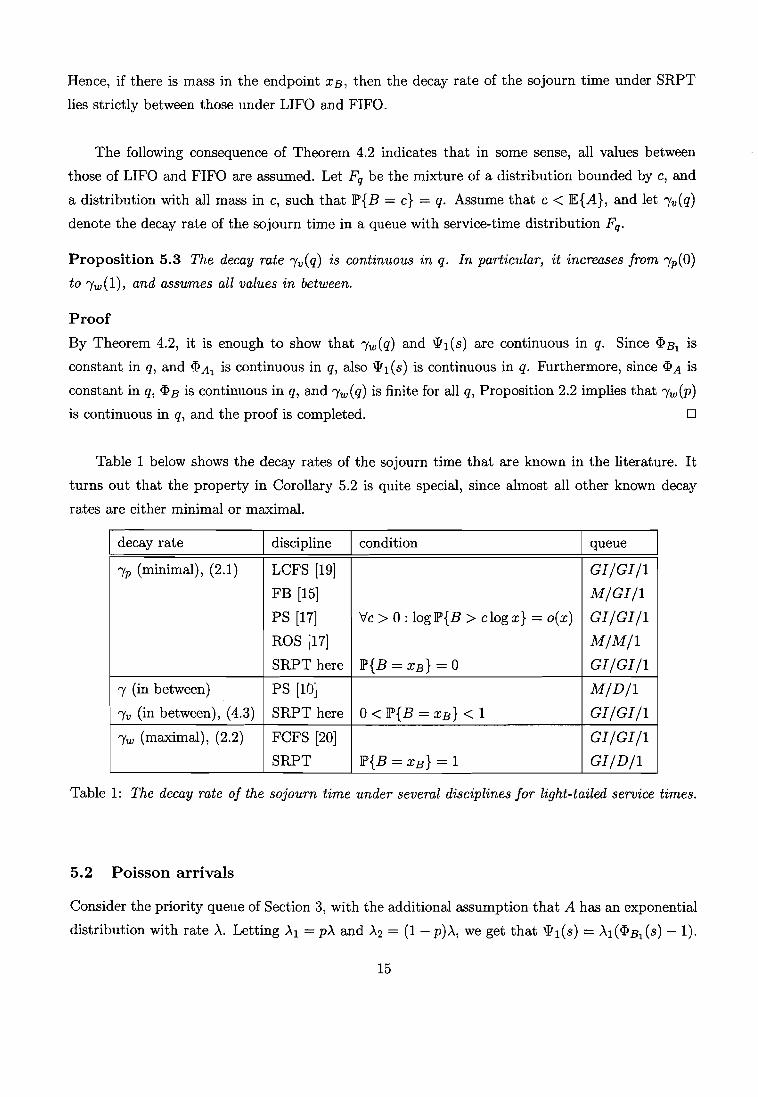
Table 1 below shows the decay rates of the sojourn time that are known in the literature. It
turns out that the property in Corollary 5.2 is quite special, since almost all other known decay
rates are either minimal or maximal.
decay rate discipline condition queue
'Yp (minimal), (2.1) LCFS [19] GI/GI/l
FB [15] M/GI/l
PS [17] 'tic> 0: loglP{B > clog x} = o(x) GI/GI/l
ROS [17] M/M/l
SRPT here lP{B = XB} = 0 GI/GI/l
'Y (in between) PS [10] M/D/l
'Yv (in between), (4.3) SRPT here O<lP{B=XB}<1 GI/GI/l
'Yw (maximal), (2.2) FCFS [20] GI/GI/l
SRPT IP'{B = XB} = 1 GI/D/l
Table 1: The decay rate of the sojourn time under several disciplines for light-tailed service times.
5.2 Poisson arrivals
Consider the priority queue of Section 3, with the additional assumption that A has an exponential
distribution with rate A. Letting Al = PA and A2 = (1- p)A, we get that WI(S) = AI(cPBI(S) -1).
15

Thus, we have
'YW2 = sup {S - Al(<:I.>B1(S) -1)}.sE[O,')'w]
Suppose that 1 - Al <:I.>Sl ('Yw) > O. Then the maximum value is attained in 'Yw and we have
This expression is rather explicit, as 'Yw is the positive solution of the equation
(5.2)
(5.3)
(5.4)
The goal of this subsection is to show that in the case of Poisson arrivals, our expression (5.3)
coincides with the expression of 'YW2 given by Abate & Whitt [1]. Assuming that lE{B1} = 1, it is
shown in [1], p. 18, that -'YW2 is the solution of 1(s) = 1IP, with
A PI ~ (1) P2f(s) = ho (s) + 92e(ZI(S)),
PI + P2 PI + P2
h~I)(s) = 1- b1(sJ = 1 - b1(s) 92e(S) = 1 - 92(S) ,S + PI - Plbl(S) ZI(S) , S921
where b1(s) is the LST of the MIGl1 busy period, 92(S) = <:I.>B2(-S) and 921 = lE{B2}.
Our expression of 'YW2 seems preferable, although we hasten to add that the form provided by
[1] is more convenient when considering the more complicated task of obtaining precise asymptotics,
as is done in [1].
We now simplify the description of 'YW2 in [1]. Since P = PI + P2, we have
1 = ~ = I(s) = PI 1- b1(s) + P2 1- 92(ZI(S)).PI + P2 P PI + P2 ZI(S) PI + P2 ZI(s)lE{B2}
Hence,
Consequently,
(5.5)
Since the LST of the busy period satisfies the fixed point equation
(5.6)
16

we can rewrite (5.5) as
and thus, using the definition of ZI (8),
Using the definition of IW in (5.4), we see that IW2 is the solution of IW = -ZI(8). We now give
an alternative expression for - ZI (8). An alternative expression for the busy period transform was
found by Rosenkrantz [21]: defining ¢(8) = Al(1- q,Bl (-8)) - 8, it holds that
(5.7)
Since q, Bl (8) is strictly increasing, it follows from (5.6) and (5.7) that ZI (8) = ¢-1 (s). Hence, IW2
is the solution of IW = _¢-I(s), and thus we obtain
which is indeed equal to our expression (5.3).
To conclude this section, we remark that for the M/G/1 queue, the decay rate IV can take on
a simple form. Suppose that 1 - Al q,~l (,w) > 0, and that °< JP>{B = x B} < 1. Then by Theorem
4.2 and the expression for IW given in (5.4), we have
IV = IW - Al(q,Bl(,W) -1) = A(q,B(,w) -1) - Al(q,Bl(,W) -1)
= A2(q,B2(,W) - 1) = AJP>{B = xB}(eXB'Yw -1).
5.3 Heavy traffic
We now examine the behavior of the decay rate IV of the SRPT sojourn time in heavy traffic. The
aim of this section is to show that the behavior of this decay rate critically depends upon whether
JP>{B = XB} > °or not. If JP>{B = XB} = 0, then IV = IP by Theorem 4.1. The results in Section
4.2 of [17] then imply that IV rv C(1- p)2 for some constant C. We now show that a fundamentally
different behavior applies if JP>{B = XB} > 0.
Since, in this case, we have a relationship with the GI / G1/1 priority queue, we consider first
the setting of Section 3. We let the service time B2 increase in such a way that P~ 1. Specifically,
we consider a sequence of systems indexed by r, such that p, AI, A 2 and B 1 are all fixed, and that
B2 = B 2(r) is such that the traffic load satisfies Pr = 1- l/r. Let Iw(Pr) denote the decay rate of
the workload in such a queue.
17
If we let O"~ < 00 be the variance of A and assume that the variance of B(r) = B 1 + B 2(r)
converges to 0"1, then it holds that for r ~ 00 (d. Corollary 3 of [12]),
(5.8)
with K = 2/(0"~ + 0"1). In particular, "Yw(Pr) 1 O. Consequently, if r is large enough, we always
have "Yw2(Pr) = "Yw(Pr) - Wl("(w(Pr)) by Theorem 3.1. Since Wl(S) ,...., p(l)s as s 10, where p(l) is
the load in the high priority queue, we obtain the following heavy-traffic result for "YW2'
Proposition 5.4 For P~ 1 as described above, we have
"YW2 ,...., K(1 - p(I))(1 - p).
Thus, also "Yv is of the order (1- p) if JP>{B = XB} > O. This behavior is notably different from
the (1 - p)2 behavior of "Yp.
6 Conditional sojourn times
Our results in Section 4 and 5 show that the decay rate "Yv for SRPT is smaller than "Yw, which is
the decay rate of the waiting (and sojourn) time under FIFO. Thus, one could say that according
to this performance measure, SRPT is worse than FIFO.
The reason that the sojourn-time decay rate under SRPT is small is apparent when taking a
closer look at the proof in Section 4.1: the sojourn time of a customer with a (very) large service
time looks like a residual busy period. However, smaller customers may have a much shorter sojourn
time. In fact, for the conditional sojourn time VSRPT(Y) = [VSRPT I B = y] under the preemptive
SRPT discipline, the following proposition holds.
Proposition 6.1 IfJP>{B = y} = 0, then logJP>{VsRPT(Y) > x},...., -"Y~x as x ~ 00.
Proof
For the lower bound, we remark that VSRPT(Y) is stochastically larger than the residual busy
period p*y in the queue with service time BY. This residual busy period has decay rate "Y~. For the
upper bound, we consider an alternative queue with generic service time BY, stationary workload
at arrival instants WYand busy period pY. Now observe that in the original queue, at any point
in time, at most one customer with original service time larger than Y has remaining service time
smaller han y. Hence, we can bound
VSRPT(Y) ~st pY(WY + Y + y),
18
where pY(x) is a busy period in the alternative queue starting with an exceptional customer of
length x. Applying the Chernoff bound, and arguing like in the proof of Proposition 2.2, we find
lim sup ~ 10gJP>{VSRPT(Y) > t} ~ - sup {s - 'lJY(s)} = -'YZ*,t-+oo t SE[O,')'wY ]
where the last equality follows from (5.1). The upper bound follows from noting that pY and p*y
have the same decay rate, and the proof is completed. 0
Suppose that B has a density, so that 'YZ is continuous in y. Then the function 'YZ strictly
decreases in Y, and converges to 'Yp > 'Yw as Y ---t 00. Further, 'Y~ ---t 00 as Y ---t 0, since 'lJY(s) ---t 0
as y ---t O. Hence, there exists a critical value y* for which 'Yf = 'Yw. Thus, when the decay rate
is used as a performance measure, one could say that FIFO is a better discipline than SRPT for
customers of size larger than y*; the fraction of customers that suffer from a change from FIFO to
SRPT is JP>{B > y*}. We now describe the behavior of y* as a function of p for p ---t 1 and p ---t O.
Proposition 6.2 Let y* = sup{y : 'Y~ 2: 'Yw}. If p ---t 1, then y* ---t XB.
Proof
Let y < XB be fixed, and let 'Y~(p) be the decay rate of pY as a function of p, and define 'Yw(p)
similarly. Since pY is a busy period in a stable queue, even when p = 1 in the original queue, we
have 'Y~(p) 2: 'Y~(1) > 0 for all p < 1. By (5.8), we have for p large enough,
Hence, for p large enough, y* 2: y. Since y < XB was arbitrary, the proof is completed. 0
Proposition 6.3 If the service time B has decay mte 'Yb E (0,00), then y* ---t 00 for p ---t O.
Proof
Let p ---t 0 by setting the generic inter-arrival time equal to rA and letting r ---t 00. Since lPr A (x) ---t 0
for all x < 0, we have lP;l(x) ---t 0 for all 0 < x < 1. Hence, for all y,
P ---t O. (6.9)
The workload does not depend on the discipline as long as the discipline is work-conserving. Further,
conditioned on it being positive, the workload under FIFO is stochastically larger than a residual
service time, which for light-tailed distributions has the same decay rate as B. Hence, we have
'Yw(p) ~ 'Yb < 00 for all p. It then follows from (6.9) that 'Yit(p) > 'Yw(p) eventually as p ---t 0 for all
y, and we can conclude that y* ---t 00 as p ---t O. 0
19

6.1 Numerical example
As an illustration, we compute y* and lP{B > y*} for the M / M /1 queue with lE{B} = 1 and arrival
rate>. (so that p = >.). Figure 1 shows the probabilities lP{B > y*} for various values of p.
0.2 r-------r----,----,----,.--------,
lP{B > y*(p)}
0.15
0.1
0.05
+++-+++++.+++ +++
+++++ ++++~ ~
++ +~ ~
++ ++ ++ +
+ +; +
+ +++ +
: ++ +
++
++
++
++
++
++
0.80.8p0.40.2
04'--_----'- --'- --'- -'--__-'
o
Figure 1: The probabilities lP{B > y*(p)} for p E (0,1) in the M/M/l queue.
From the figure, it is clear that y* becomes very large under low and high loads. But even for
moderate values of p it is clear that about 85 percent of the customers would prefer (from a large
deviations point of view) SRPT over FIFO.
7 Conclusions
To conclude the paper, we summarize our results. For the GI/GI /1 queue with light-tailed service
times, we obtained expressions for the logarithmic decay rate of the tail of the workload, the busy
period, the waiting time and sojourn time of low-priority customers in a priority queue, and the
sojourn time under the (preemptive and non-preemptive) SRPT discipline.
For the sojourn time under SRPT, it turns out that there are three different regimes, namely
for service times with no mass, with some mass and with all mass in the endpoint of the service-time
distribution. In the first case the decay rate is minimal among all work-conserving disciplines, in
the last case it is maximal, but if there is some mass in the endpoint, then the decay rate lies strictly
in between these two. The large-deviations results for the unconditional sojourn times suggest that
a switch from FIFO to SRPT is not advisable. The results in Section 6 show that this suggestion
is only valid for very large service times: in the M / M /1 queue, at least about 85 percent of the
customers would benefit from a change from FIFO to SRPT.
20

There are several topics that are interesting for further research. First of all, large deviations
for the queue length under SRPT are not well understood. A second problem is to obtain precise
asymptotics for the tail behavior of the low-priority waiting time, or perhaps even the sojourn
time. Finally, it would be interesting to compare conditional sojourn times of FIFO and PS from a
large-deviations point of view. It is not clear to us which discipline performs better, and what the
influence of the job size might be.
Acknowledgments
We would like to thank Marko Boon for helping us out with the numerics in Section 6.1, and Ton
Dieker and Michel Mandjes for several useful comments.
References
[1] Abate, J., Whitt, W. (1997). Asymptotics for MIG/1low-priority waiting-time tail probabil
ities. Queueing Systems 25, 173-233.
[2] Asmussen, S. (2003). Applied Probability and Queues. Second edition. Springer.
[3] Baccelli, F., Bremaud, P. (2003). Elements of Queueing Theory. Third edition. Springer.
[4] Bansal, N., Harchol-Balter, M. (2001). Analysis of SRPT scheduling: investigating unfairness.
Proceedings of A eM Sigmetrics, 279-290.
[5] Bansal, N. (2004). On the average sojourn time under MIMI1 SRPT. Operations Research
Letters 33, 195-200.
[6] Bansal, N., Gamarnik, D. (2005). Handling load with less stress. Submitted for publication.
[7] Borst, S.C., Boxma, O.J., Nunez-Queija, R., Zwart, A.P. (2003) The impact of the service
discipline on delay asymptotics. Performance Evaluation 54, 177-206.
[8] Cox, D., Smith, W. (1961). Queues. Methuen.
[9] Dembo, A., Zeitouni, O. (1998). Large Deviations Techniques and Applications. Springer.
[10] Egorova, R., Zwart, R, Boxma, O.J. (2005). Sojourn time tails in the MIDI! Processor
Sharing queue. Report PNA-R05xx, CWI, Amsterdam. Submitted for publication.
[11] Ganesh, A., O'Connell, N., Wischik, D. (2003). Big Queues. Springer.
[12] Glynn, P., Whitt, W. (1994). Logarithmic asymptotics for steady-state tail probabilities in a
single-server queue. Journal of Applied Probability 31A, 131-156.
21

[13] Harchol-Balter, M., Schroeder, B., Bansal, N., Agrawal, M. (2003). Sizebased scheduling to
improve web performance. ACM Transactions on Computer Systems 21, 207-233.
[14] Kingman, J.F.C. (1964). A martingale inequality in the theory of queues. Proceedings of the
Cambridge Philosophical Society 59, 359-361.
[15] Mandjes, M., Nuyens, M. (2005). Sojourn times in the M/G/l FB queue with light-tailed
service times. Probability in the Engineering and Informational Sciences 19, 351-361.
[16] Mandjes, M., Van Uitert, M. (2005). Sample path large deviations for tandem and priority
queues with Gaussian input. Annals of Applied Probability 15, 1193-1226.
[17] Mandjes, M., Zwart, B. (2004). Large deviations for sojourn times in processor sharing queues.
Queueing Systems, under revision.
[18] Nuiiez-Queija, R. (2000). Processor-Sharing Models for Integrated-Service Networks. PhD the
sis, Eindhoven University of Technology.
[19J Palmowksi, Z., Rolski, T. (2004). On busy period asymptotics in the GI/GI/l queue. Sub
mitted for publication, available at
http://www.math.uni.wroc.pl/-zpalma/publication.html
[20J Ramanan, K., Stolyar, A. (2001). Largest weighted delay first scheduling: large deviations and
optimality. Annals of Applied Probability 11, 1-48.
[21J Rosenkrantz, W. (1983). Calculation of the Laplace transform of the length of the busy period
for the MIG/l queue via martingales. Annals of Probability 11,817-818.
[22] Schrage, L. (1968). A proof of the optimality of the shortest remaining service time discipline.
Operations Research 16, 670--690.
22