a lagrangian analysis of the impact of transport and

HAL Id: hal-00328458https://hal.archives-ouvertes.fr/hal-00328458

Submitted on 25 Aug 2006

HAL is a multi-disciplinary open accessarchive for the deposit and dissemination of sci-entific research documents, whether they are pub-lished or not. The documents may come fromteaching and research institutions in France orabroad, or from public or private research centers.

L’archive ouverte pluridisciplinaire HAL, estdestinée au dépôt et à la diffusion de documentsscientifiques de niveau recherche, publiés ou non,émanant des établissements d’enseignement et derecherche français ou étrangers, des laboratoirespublics ou privés.

A Lagrangian analysis of the impact of transport andtransformation on the ozone stratification observed in

the free troposphere during the ESCOMPTE campaignAugustin Colette, Gérard Ancellet, Laurent Menut, Steve R. Arnold

To cite this version:Augustin Colette, Gérard Ancellet, Laurent Menut, Steve R. Arnold. A Lagrangian analysis of the im-pact of transport and transformation on the ozone stratification observed in the free troposphere duringthe ESCOMPTE campaign. Atmospheric Chemistry and Physics, European Geosciences Union, 2006,6 (11), pp.3503. �hal-00328458�

https://hal.archives-ouvertes.fr/hal-00328458

https://hal.archives-ouvertes.fr

Atmos. Chem. Phys., 6, 3487–3503, 2006www.atmos-chem-phys.net/6/3487/2006/© Author(s) 2006. This work is licensedunder a Creative Commons License.

AtmosphericChemistry

and Physics

A Lagrangian analysis of the impact of transport andtransformation on the ozone stratification observed in the freetroposphere during the ESCOMPTE campaign

A. Colette1, G. Ancellet1, L. Menut2, and S. R. Arnold3

1Service d’Aeronomie/Institut Pierre-Simon Laplace, Centre National de la Recherche Scientifique, Universite Pierre etMarie Curie, 4, place Jussieu, P.O. Box 102, 75252 Paris Cedex 05, France2Laboratoire de Meteorologie Dynamique/Institut Pierre-Simon Laplace, Centre National de la Recherche Scientifique, EcolePolytechnique, 91128 Palaiseau Cedex, France3Institute for Atmospheric Science, School of Earth and Environment, University of Leeds, Leeds, LS2 9JT, UK

Received: 11 November 2005 – Published in Atmos. Chem. Phys. Discuss.: 21 March 2006Revised: 28 June 2006 – Accepted: 3 August 2006 – Published: 25 August 2006

Abstract. The ozone variability observed by troposphericozone lidars during the ESCOMPTE campaign is analyzedby means of a hybrid-Lagrangian modeling study. Transportprocesses responsible for the formation of ozone-rich layersare identified using a semi-Lagrangian analysis of mesoscalesimulations to identify the planetary boundary layer (PBL)footprint in the free troposphere. High ozone concentrationsare related to polluted air masses exported from the IberianPBL. The chemical composition of air masses coming fromthe PBL and transported in the free troposphere is evaluatedusing a Lagrangian chemistry model. The initial concentra-tions are provided by a model of chemistry and transport.Different scenarios are tested for the initial conditions andfor the impact of mixing with background air in order to per-form a quantitative comparison with the lidar observations.For this meteorological situation, the characteristic mixingtime is of the order of 2 to 6 days depending on the initialconditions. Ozone is produced in the free troposphere withinmost air masses exported from the Iberian PBL at an averagerate of 0.2 ppbv h−1, with a maximum ozone production of0.4 ppbv h−1. Transport processes from the PBL are respon-sible for an increase of 13.3 ppbv of ozone concentrations inthe free troposphere compared to background levels; about45% of this increase is attributed to in situ production duringthe transport rather than direct export of ozone.

Correspondence to:A. Colette([email protected])

1 Introduction

Transport and transformation of photochemically reactivespecies in the troposphere are topics of sustained attention.Ozone is one of the main oxidants in the atmosphere; itis either produced in the stratosphere, the planetary bound-ary layer (PBL) or the free troposphere (FT). In the PBL,ozone precursors include biogenic and anthropogenic emis-sions (from both transports and industrial activities). Oncein the troposphere, ozone can be transported over long dis-tances enhancing local pollution in remote places (Zhang andTrivikrama Rao, 1999) or perturbing fragile equilibrium inpristine areas (e.g. when transported to the poles, Eckhardt etal., 2003). In addition, increased background ozone concen-trations in the troposphere play an important role in globalclimate change because of its radiative properties (Bernstenet al., 1997).

In this paper, we focus on transport processes from thePBL and their impact on free tropospheric ozone variability.Cotton et al. (1995) suggest that the PBL is vented towardthe FT 90 times per year on a global scale. This coupling oc-curs through a wide spectrum of transport mechanisms: lo-cal circulations – either orographic (Henne et al., 2004) orsea breezes (Bastin and Drobinski, 2006), convective sys-tems (Hauf et al., 1995) or frontal systems (Cooper et al.,2002). If such transport processes occur above polluted ar-eas, they export ozone or its precursors to the FT.

The European ESCOMPTE program (Experience sur Sitepour Contraindre les Modeles de Pollution Atmospheriqueet de Transport d’Emissions, Cros et al., 2004) was designedto gather measurements in order to better assess atmospheric

Published by Copernicus GmbH on behalf of the European Geosciences Union.

3488 A. Colette et al.: Impact of transport and transformation on ozone variability

chemistry transport models (CTM). Many publications re-lated to the ESCOMPTE campaign are included in Cros andDurand (2005). During this campaign, several troposphericozone profilers were operated, so that the ozone stratifica-tion above the PBL and its temporal evolution are well doc-umented (Ancellet and Ravetta, 2005).

The goal of the present study is first to identify the trans-port mechanisms responsible for the observed ozone vari-ability in the FT, and second to assess the photochemicaltransformation occurring during the transport. Three modelsare coupled to achieve a hybrid-Lagrangian reconstruction ofthe observed ozone variability. A mesoscale non-hydrostaticmodel is used to compute high-resolution backtrajectories inorder to identify air masses coming from the polluted PBL.A CTM designed for PBL simulations allows the evaluationof the chemical composition of selected air masses at thetime and place of export from the PBL. Then, photochem-ical transformation during the transport is computed using aLagrangian chemistry model. This approach leads to a re-construction of the ozone variability that matches observa-tions and allows the discussion of the impact of mixing withbackground air as well as the quantification of ozone pro-duction rates for different transport pathways. The advan-tages of such a Lagrangian approach compared to Euleriansimulations are twofold. First, at similar computational cost,scales resolved with a Lagrangian model are smaller (Norton,1994), which is of crucial importance considering the largeozone variability observed during ESCOMPTE. Second, bytracking air masses, it allows a better understanding of theirtemporal evolution during the transport.

The field campaign, ozone lidar measurements and thegeneral synoptic context are presented in Sect. 2. Section 3addresses the results of the hybrid-Lagrangian analysis of theobserved tropospheric ozone variability. A mesoscale mod-eling study leads to the identification of transport processesdiscussed in Sect. 3.1. The influence of photochemical trans-formation is investigated in Sects. 3.2 and 3.3. First, we de-scribe a purely advective reconstruction of the ozone vari-ability with a reverse domain filling method. Second, a La-grangian chemistry model is used to simulate the transforma-tion occurring during the transport in the free troposphere;so that a quantitative comparison with lidar observations caneventually be conducted.

2 The ESCOMPTE campaign

2.1 General description

The ESCOMPTE campaign (Cros et al., 2004) took place inJune and July 2001 in the Aix-Marseille area (South-EasternFrance). The region is densely inhabited; iron, steel, petro-chemistry factories and oil refineries are located around theBerre pond. The area is thus highly exposed to anthropogenicemissions of pollutants both from transports and industrial

activities. The local vegetation is also an important source ofvolatile organic compounds.

In the ESCOMPTE region, a wide range of dynamic forc-ing plays a role in trace gases circulation. Within the PBL,valley breezes develop in the Alpilles and Luberon massifsand in the Durance and Rhone valleys. Strong sea breezesthat can penetrate as far as 100 km inland are frequently ob-served (Bastin et al., 2005; Puygrenier et al., 2005). At night,land breezes can store polluted air masses above the mar-itime boundary layer and thus build reservoirs of aged pol-luted air that may return onshore on the following day (Gan-goiti et al., 2001; Ancellet and Ravetta, 2005). Above thePBL, local circulations have a limited impact and synopticand mesoscale processes predominate. When a trough is lo-cated over the Balkan countries, the Alps and Massif Centralchannel a strong northerly flow (the Mistral) that shall carryanthropogenic trace gases from the Lyons and Paris agglom-erations (Corsmeier et al., 2005). In the following, we willdiscuss in details how intra-European transport can importpolluted air masses to the ESCOMPTE domain. Last, thisarea is exposed to the long-range transport of polluted airmasses; Lelieveld et al. (2002) suggest that air masses trans-ported through the Westerlies above the Northern AtlanticOcean during summer often veer to South-Eastern Francewhen reaching the European continent.

During the campaign, measurements included an en-hanced network of ground based stations, balloon sound-ings, constant volume balloon flights, sodars, radars, windand ozone lidars and 6 instrumented aircrafts. In the presentpaper, we will primarily use measurements performed by theService d’Aeronomie (CNRS, France) with the troposphericlidar ALTO (Ancellet and Ravetta, 1998).

2.2 Selection of the time frame

Four intensive observation periods (IOP) were conductedduring the ESCOMPTE campaign. We performed a prelim-inary analysis to define the most interesting case studies inthe framework of the coupling between the PBL and the FT.IOP2 (between 21 and 26 June) was recognized as an appro-priate period because of its long duration, the variability ofmeteorological conditions monitored and the quality of thedataset available. A first trajectory analysis was performedusing large-scale wind fields for the whole IOP2 to target thetime frame when mesoscale transport influenced the tropo-spheric ozone variability in the ESCOMPTE area. For thispurpose, we used the Lagrangian particle dispersion modelFLEXPART 5.1 (Stohl et al., 1998). The model was drivenby 6-hourly ECMWF operational analyses (T511L60) inter-leaved with forecasts every 3 h (ECMWF, 1995). The se-lected domain extended from 100 W to 40 E of longitude and20 N to 80 N of latitude. In addition to advective transportat the scale of the global reanalyses, the FLEXPART modelaccounts for subgrid-scale orographic and convective vent-ing (Stohl et al., 2005), and its efficency at discriminating

Atmos. Chem. Phys., 6, 3487–3503, 2006 www.atmos-chem-phys.net/6/3487/2006/

A. Colette et al.: Impact of transport and transformation on ozone variability 3489

air masses coming from the PBL or from the tropopause re-gion has been demonstrated in the past, e.g. by Stohl andTrickl (1999).

Ozone measurements performed on 21 and 22 June arepresented in Ancellet and Ravetta (2005). The FLEXPARTanalysis shows that positive and negative ozone anomaliesobserved these days are associated to synoptic transport pro-cesses active above the Northern Atlantic Ocean.

According to the FLEXPART simulations, the highestproportion of free tropospheric air observed above the ES-COMPTE area coming from the European PBL (and thuspossibly influenced by continental emissions) is found be-tween 23 and 26 June. During this period, 33% of the freetroposphere below 5 km a.s.l. correspond to air masses re-cently extracted from the PBL, mostly above the IberianPeninsula. Consequently, the 23 to 26 June period is wellsuited for an analysis of the impact of mesoscale couplingbetween the PBL and the FT on the ozone variability.

According to the FLEXPART model, the selected ozone-rich air masses were free of any stratospheric signature. Thehypothesis of a stratospheric origin is further discarded byconsidering aerosol backscatter measurements of the ALTOlidar presented in Ancellet and Ravetta (2005) that is clearlyabove typical values expected for stratospheric air masses.In addition, carbon monoxide measurements performed onboard the Dornier aircraft (Saıd et al., 2005) indicate con-centrations of about 150 ppbv in the vicinity of the selectedtropospheric layers on 24th June. This value is in the rangeexpected for aged polluted air masses. On the contrary, in thePBL, CO concentrations exceed 200 ppbv for local pollutionplumes and is of the order of 100 ppbv for clean air masses.

2.3 Synoptic situation

On 23 June a Mistral regime ends. During the follow-ing days, the axis of a strong ridge extending from Mo-rocco to Norway moves slowly eastward over France andis associated with weak northwesterly to westerly winds inthe free troposphere (see the meteorological analyses of theDeutscher Wetterdienst for 24 June at 500 hPa on Fig. 1a).In the PBL, sea breezes develop daily. On 26 June, the windregime turns southwesterly as the ridge moves eastward and asurface low pressure system develops South of Ireland. Con-sequently, this day is discarded from the following analysis.

At the surface, the analyses (e.g. Fig. 1b) show that a ther-mal low develops daily above Spain between 20 and 25 June.Mill an et al. (1997) explain in details how such a situationfavors the export of PBL air to the lower FT; orographic cir-culations and sea breezes playing an important role inlandand along the coast, respectively. These two types of lo-cal circulations can also be observed in conjunction alongmountainous coastlines. Millan et al. (1997) also mentionthe importance of the convective activity. METEOSAT in-frared images suggest that shallow convection occurred be-tween 21 and 25 June above Spain. However, it did not orga-

nize in large Mesoscale Convective Systems (MCS); one ofthe strongest events is shown on Fig. 1c.

To sum up, the thermal low above Spain exports PBL airto the FT where it is advected to the ESCOMPTE domain bythe weak westerly flow. The paths followed by air massesarriving above the ALTO measurement site below 5 km be-tween 23 and 25 June are presented on Fig. 1d. Exclusivelyair parcels coming from the PBL are displayed; their trajecto-ries illustrate well the synoptic situation summarized above.

2.4 Ozone profiling

The most complete coverage of free tropospheric ozone wasperformed by ground-based lidars. Two instruments wereoperated during the campaign. The Service d’Aeronomie(CNRS, France) operated the ALTO lidar at Aix-les-Milles(5.48 E, 43.58 N, 110 m a.s.l.). This instrument is based onthe DIAL technique (DIfferential Absorption Lidar) usingtwo wavelength pairs: 266–289 nm and 289–316 nm. Thefirst pair is very well suited for measurements at short dis-tances (below 1.5 km) although no reliable measurement canbe performed below 0.5 km. The second pair allows mea-surements up to 4–5 km. The 316 nm signal is used for re-trieving the aerosol backscattering ratio. Ozone is biasedwhen estimated by the DIAL technique in the presence ofhigh aerosol load. Consequently an additional correction isperformed using the backscatter estimate at 316 nm. Whenaerosols concentration is too high, uncertainty is so impor-tant that ozone measurements are discarded. Details on theinstrument are given in Ancellet and Ravetta (1998). Aerosolmeasurements, ozone correction and validation of the mea-surements performed during ESCOMPTE can be found inAncellet and Ravetta (2005). During the campaign, the spa-tial and temporal variability of tropospheric ozone was alsodocumented by airborne and balloon borne instruments. Acomparative analysis of in situ and remote sensing ozonemeasurements is described in Ancellet and Ravetta (2005)who show how to relate spatial variability revealed by theaircrafts with the temporal variability of the ground-based li-dar.

The ALTO record is sparse, that is why lidar measure-ments by the Ecole Polytechnique Federale de Lausanne(EPFL, Switzerland) are also presented here (Simeonov etal., 2004). The instrument was based at Saint-Chamas(35 km west of Aix-les-Milles, 5.04 E, 43.32 N, 210 m a.s.l.).The EPFL record presents a good temporal continuity. Theinstrumental setup is very similar to the ALTO lidar how-ever no correction of ozone in the presence of aerosols isperformed. For both instruments, ozone measured above4000 m a.g.l. is discarded because of the low signal to noiseratio.

Ozone records are presented on Figs. 2a and b. At first or-der, even if the instruments are not co-localized, these twodatasets present some similar patterns. For both records,below 1500 m a.s.l. important local pollution plumes are

www.atmos-chem-phys.net/6/3487/2006/ Atmos. Chem. Phys., 6, 3487–3503, 2006


Fig. 1. Meteorological analyses of the Deutscher Wetterdienst for 24 June 2001 12:00 UT, geopotential at 500 hPa(a), and sea level pressure(b). METEOSAT infrared image for 24 June 12:00 UT(c). Mesoscale backtrajectories from the ALTO measurement site associated toPBL-FT coupling(d).

observed on 24 and 25 June. The synoptic situation is an-ticyclonic on these two days, which favors the developmentof sea breezes that can transport ozone produced in the leeof urban or industrial areas to the measurement sites. Re-garding free tropospheric ozone variability, the most strikingpattern is a large enhanced ozone structure observed betweenthe afternoon of 23 June and the morning of 25 June centeredat 2500 m a.s.l. Other interesting patterns include the lowozone concentrations measured in the morning of 23 Juneand an ozone depleted layer centered at 1500 m a.s.l. on 24June.

More quantitatively, we found a +10 ppbv difference onaverage between EPFL and ALTO data for the 23 to 25 Juneperiod. To our understanding, the lack of aerosol correctionin the EPFL algorithm should explain this offset. Conse-quently, EPFL data will be used for the qualitative compar-ison with modeled ozone variability, while ALTO measure-ments are preferred for the quantitative comparison of ozoneconcentrations (note that for a more appropriate reading ofFig. 2, we chose to account for this offset in the correspond-ing color scales).

3 Modeling analyses

The modeling analysis includes three steps: the identifi-cation of transport pathways with a 3-D mesoscale model(MesoNH); the estimation of trace gases concentrations inthe PBL when the air mass is exported to the FT using aCTM (CHIMERE); the analysis of the photochemical trans-formation during the transport using a Lagrangian chemistrymodel (CiTTyCAT).

3.1 Transport pathways

3.1.1 Description of the MesoNH model

MesoNH is a non-hydrostatic mesoscale model developedjointly at Laboratoire d’Aerologie (CNRS, France) and atthe French Centre National de Recherche Meteorologiques(Meteo-France). Complete description of the model is givenin Lafore et al. (1998); the version used here is 4.5.1. Thedomain is centered on Southern France with 72×72 30 km-wide grid cells. The vertical grid is terrain following with 48levels ranging from 60 m to 19 km a.s.l., including 10 levelsbelow 1 km. The simulation is initialized and relaxed at the



boundaries toward T511L60 ECMWF operational analyses(ECMWF, 1995). 7 simulations lasting 30 h each with 6 h ofspin up were performed between 19 and 25 June 2001.

In these simulations semi-Lagrangian tracking of airparcels is activated (Gheusi and Stein, 2002). This methodconsists basically in modeling an additional variable in theEulerian simulation: the 3-D field of the initial coordinates ofthe grid cells at the initialization of the run. Consequently, ateach timestep, the initial position of every grid cell is knownthroughout the domain. In addition to advection, these airparcels undergo sub-grid scale processes such as turbulentmixing. In this study, the semi-Lagrangian analysis is usedto compute backtrajectories that are more reliable for docu-menting mesoscale processes than classical Lagrangian tra-jectories, where wind fields are interpolated in the advectionprocess.

3.1.2 Mesoscale trajectories

We mentioned in Sect. 2.2 that, according to the FLEX-PART model, most air masses arriving above the ALTO mea-surement site are coming from the Iberian PBL. Howeverthis trajectory analysis can be significantly improved usingthe mesoscale simulation. Mesoscale backtrajectories werecomputed every hour between 23 and 25 June. Their end-ing points correspond to the ALTO measurement site every250 m between the surface and 5000 m a.s.l. Trajectories arerun for 3 days back in time. Indeed, considering the ex-tension of the domain and free tropospheric wind velocities,the parcels leave the domain within 3 days if they remain inthe FT. Turbulent kinetic energy (TKE) is interpolated fromthe mesoscale simulation along the trajectories to diagnoseif air masses are coming from the PBL. If the TKE exceeds0.2 m2 s−2 (Gheusi et al., 2004) for more than 3 contiguoushours of time, the air mass is considered as being inside thePBL. However, an additional test is required to discard TKEgenerated by clear air turbulence, i.e. when high TKE levelsare modeled above 3000 m in the vicinity of mountain rangesin relation with lee waves breaking. At the altitudes consid-ered (below 5000 m a.s.l.), turbulence related to shearing inthe jet streak does not occur. With this TKE criterion wefound that 48% of the trajectories are coming from the PBLamong a total of about 1350 trajectories.

The results of the trajectory analysis are synthesized onFig. 3. If during the 72 h before arriving in the ESCOMPTEarea, the trajectory has been in the PBL, a square is plotted onthe top panel at the time and altitude of arrival of the trajec-tory. On the second panel, the square is plotted at the locationof export from the PBL. The color of the squares correspondto the time the air parcels spent in the FT. When this time isshorter than 2 h, we can conclude that the corresponding airmass is influenced by the local PBL. Every afternoon, suchair masses are detected above the observation site, in relationwith the diurnal cycle of the PBL. This evolution of the localPBL is correlated with the enhanced ozone concentrations

23/06/01 24/06/01 25/06/01 26/06/010

500

1000

1500

2000

2500

3000

3500

4000

4500

5000

Altit

ude

(m a

sl)

O3 (ppbv)

20

30

40

50

60

70

80

90

100

23/06/01 24/06/01 25/06/01 26/06/010

500

1000

1500

2000

2500

3000

3500

4000

4500

5000

Altit

ude

(m a

sl)

O3 (ppbv)

30

40

50

60

70

80

90

100

110

Fig. 2. Tropospheric ozone profiles measured by the ALTO(a) andEPFL (b) lidars between 23 and 25 June in the ESCOMPTE area.Color scales differ to account for the 10 ppbv offset between theinstruments.

measured by the lidar at mid-day in the 1000–1500 m alti-tude range which suggest a connection with local pollutionplumes. Among the trajectories arriving above 750 m a.s.l.,17% were extracted from the PBL in the ESCOMPTE regionand 31% are associated to an export from the Iberian PBLone to two days before the end of the trajectory.

The main free tropospheric ozone-rich layer centeredaround 2500 m on 24 June (Fig. 2) matches well with thefootprint of air masses exported from the distant PBL onFig. 3a. The trajectory analysis shows that this layer isconstituted of air masses coming from widespread loca-tions above Spain; but the relative homogeneity of a sin-gle tracer such as ozone in these air masses is not necessar-ily contradictory with their very variable geographical ori-gins. Compared to this event, observed ozone concentrationsare slightly lower after 14:00 UT on 25 June in the altituderange 2500–3000 m. This feature can be related to the het-erogeneity of the origins of the air masses according to themesoscale model. Using global GCM simulations, Dufouret al. (2005), attributed the decrease of ozone concentrationsobserved on this day to vertical mixing with a tropical airmass in the upper layers. This hypothesis on the vertical



23/06/01 24/06/01 25/06/01 26/06/010

500

1000

1500

2000

2500

3000

3500

4000

4500

5000Al

titud

e (m

asl)

Time in FT (hours)

0

10

20

30

40

50

60

−10 −8 −6 −4 −2 0 2 4 6

36

38

40

42

44

46

0

10

20

30

40

50

60

70

80

Fig. 3. Footprint of air masses with a PBL origin arriving above theALTO measurement site according to the mesoscale backtrajecto-ries. A square is plotted for each trajectory coming from the PBL.The color of the square corresponds to the time the air parcel spentin the free troposphere before arriving in the ESCOMPTE area. Toppanel: squares are plotted at the ending point of the trajectory (timeand altitude above the lidar); bottom panel: squares are plotted atthe location of extraction from the PBL. A red circle is plotted atthe ALTO measurement site.

mixing is somewhat supported by the heterogeneity revealedby our analysis. Low ozone concentrations measured by li-dar on 23 June and in the morning of the 24th at moderatealtitudes (around 1500 m), correspond to air masses exemptfrom any PBL signature. These trajectories are coming fromthe troposphere above the Northern Atlantic Ocean which isconsistent with their relatively low ozone content (Reeves etal., 2002). The same conclusion holds for high altitude airmasses (above 3000 m) observed in the afternoon of 24 Juneand 25 June. To sum up, this analysis shows that positiveozone anomalies observed by lidar above 1500 m a.s.l. be-tween 23 June 12:00 UT and 25 June 23:00 UT are syn-chronized with air masses having undergone export from thePBL, while ozone depleted layers are associated to aged freetropospheric air masses.

In the following, we will attempt to quantify the ozonecontent of air masses exported from the PBL according tothe trajectory analysis. Prior to this step, the precise fractionof lidar data corresponding to air masses transported fromthe Iberian PBL must be selected. Possible mismatches inthe timing between the model and the observations prohibit astraightforward comparison (Methven et al., 2001). Methvenet al. (2003) propose a correction procedure using comple-mentary in situ measurements such as the specific humidityand the equivalent potential temperature; but in our case theonly available quantities above the lidar are the ozone con-centrations and the aerosol backscattering ratio. Using largescale FLEXPART simulations we ensured that neither longrange transport of pollutants nor stratospheric intrusions didplay any role. So ozone-rich layers whose temporal and spa-tial extension is similar to the PBL footprint given on Fig. 3are selected as coming from the PBL (see the black contourson Fig. 2a). The only exception is found on 23 June whenwe discarded two layers (centered at 2500 m and 1500 m) be-cause we did not find any matching evidence of PBL exportwith the mesoscale model.

3.1.3 Transport processes analysis

Local processes play an important role in trace gases dis-tribution in the ESCOMPTE area. In the framework of thecampaign, Bastin et al. (2005), Kahltoff et al. (2005) or Puy-grenier et al. (2005) propose analyses of PBL processes thatmay lead to an export to the FT. In this paper, we decided tofocus on free tropospheric air masses extracted from the dis-tant PBL, i.e. air masses that have undergone transport andtransformation in the free troposphere.

Figure 3b shows the very large variability of geographicalorigins of air masses arriving in the FT above the ALTO lidar.To synthesize the information and identify the main transportpathways, the trajectories were clustered using the k-meansmultivariate clustering technique (Mac Queen, 1967). Eachtrajectory is characterized by its date, latitude and longitudeof extraction from the PBL, and its date and altitude of ar-rival. To maximize the consistency of the clusters of trajec-tories we imposed a high number of clusters (about 20).

The clusters are displayed on Fig. 4 in a similar way ason Fig. 3a. Here, colors and labels correspond to the clus-ters of trajectories and exclusively air masses extracted fromthe distant PBL are presented. This way, one can infer therelation between air masses arriving above the ALTO mea-surement site and clusters of air masses listed on Table 1.Table 1 summarizes the characteristics of each cluster of tra-jectories, including the date and approximate location of ex-traction. We find that export from the Iberian PBL occurreddaily during this period and that these processes took placeat very widespread locations above Spain. The consistencyof the clusters can be inferred from the root mean square dis-tance (RMS) between the locations of uptake from the PBLfor the trajectories belonging to each cluster. The number of



06/23 06/24 06/25 06/260

500

1000

1500

2000

2500

3000

3500

4000

4500

5000

6 6

22 6 6 11 11 15

1 1 1 1 1 1 1 1 22 15 6 22 10 6 15 11 6 15 15 15 15 15 15 15 11 11 19

7 22 1 1 1 1 1 1 1 1 1 1 6 6 6 6 6 6 6 6 10 10 10 10 10 10 10 1 8 8 6 11 11 15 19 19

7 7 22 1 1 1 1 1 1 1 1 1 4 4 6 6 6 11 6 6 8 10 10 10 10 1 8 8 8 1 1 8 8 8 11 8 15 19 19 19

7 7 7 7 7 20 1 1 1 1 4 4 4 4 4 4 4 4 2 2 2 11 11 11 10 10 10 1 1 8 8 8 8 8 8 11 8 13 13 13

17 16 16 16 7 7 7 7 7 20 20 20 1 1 1 1 4 4 4 4 4 4 4 4 17 2 2 2 2 2 11 2 1 1 1 1 8 13 13 13 19

16 16 7 7 7 20 16 7 20 20 20 9 9 9 5 5 4 4 4 4 4 2 2 2 2 2 2 2 2 2 5 5 14 14 13 13 13 14 12

17 16 17 17 16 16 9 9 20 9 16 9 21 5 5 5 5 5 5 2 2 14 2 2 2 2 2 5 5 14 13 14 12 12

17 17 16 18 18 21 9 9 9 9 9 21 5 5 5 5 5 5 2 17 14 14 2 5 5 14 14 13 12 12 12 12 12

17 16 18 18 17 21 9 9 9 21 3 3 3 3 3 3 3 17 14 5 14 12

18 18 18 21 7 23 21 3 3 3 3 3 3

18 18 18 3 23 23 21 3 3 3 3 12

3 23 23 3 3 3 3 3

Altit

ude

(m a

sl)

Cluster

0

2

4

6

8

10

12

14

16

18

20

22

Fig. 4. Same as Fig. 3a for air masses extracted from the PBL outside of the ESCOMPTE region. Labels and color shading correspond tothe references of the clusters of trajectories (see Table 1).

trajectories belonging to each cluster is also given to assessthe significance of the clusters.

Modeled convective available potential energy (CAPE) isused to diagnose if convection could be responsible for theexport to the FT. METEOSAT images suggest that convec-tion did not organized in large MCS. Consequently in areaswhere modeled CAPE is high, export from the PBL remainslimited to shallow convection. When CAPE levels are negli-gible, the most likely processes playing a role in the export tothe free troposphere are thermal circulations. As mentionedin Sect. 2.3, depending on the location of export, these ther-mal circulations can be purely orographic, sea breezes, or acombination of both.

For most clusters, the export occurred in the afternoon –when convection and thermal circulations reach their peakefficiency in terms of PBL venting. The only trajectories thatleft the PBL in the morning belong to clusters 3 to 6. Theycorrespond to air masses where ozone production is maxi-mum as will be discussed in Sect. 3.5.

Using Eulerian chemistry simulations, Cousin et al. (2005)suggest that free tropospheric ozone variability measured bythe ALTO lidar is influenced by air masses coming from theBarcelona area. The fact that they did not detect any trans-port processes from more distant places above Spain is prob-ably related to the limited extent of their simulation domain.Dufour et al. (2005) propose another explanation for the freetropospheric ozone variability. They focus on CTM simula-

tions and, by shutting down the two-way coupling betweenfour nested domains, they discuss the origin of ozone-richlayers observed by the ALTO lidar on 24 and 25 June. Theysuggest stratospheric intrusions played an important role be-cause some ozone-rich layers are not simulated when cli-matological boundary conditions are used above 5000 m. Infact, an export from the PBL followed by tropospheric trans-port above 5000 m would give the same results. At the conti-nental scale, the resolution of their CTM is similar to that ofECMWF analyses used in the FLEXPART simulation pre-sented above. According to the FLEXPART model, manyair masses coming from the Iberian PBL were indeed trans-ported at about 5000 m of altitude.

3.2 Trace gases concentrations in the Iberian PBL

At this stage, we have shown a relationship between freetropospheric ozone-rich air masses observed in the ES-COMPTE area and modeled air masses exported from theIberian PBL. The chemical composition of these air masseswhen they left the PBL can be evaluated using CTM simula-tions. In this study we used the model CHIMERE (versionV200501G).



06/23 06/24 06/25 06/260

500

1000

1500

2000

2500

3000

3500

4000

4500

5000

Altit

ude

(m a

sl)

10

20

30

40

50

60

70

80

90

100

110

06/23 06/24 06/25 06/260

500

1000

1500

2000

2500

3000

3500

4000

4500

5000

Altit

ude

(m a

sl)

0

0.5

1

1.5

2

2.5

3

3.5

4

4.5

Fig. 5. Reverse domain filling of ozone(a) and NOx (b) concentrations (in ppbv) for air masses arriving above the ALTO lidar and comingfrom the Iberian PBL. Concentrations at the date and location of export from the PBL are interpolated from the CHIMERE simulation.

3.2.1 Description of the CHIMERE model

The model is described in Vautard et al. (2001) and the vali-dation of continental scale simulations is given by Schmidtet al. (2001). The most up to date information regardingthe model can be found athttp://euler.lmd.polytechnique.fr/chimere/.

The CTM is driven by MM5 meteorological fields (Vau-tard et al., 2005). Surface emissions are those of the annualEMEP inventory (http://www.emep.int) converted to hourlyfluxes using the GENEMIS database (GENEMIS, 1994).The general circulation model LMDz-INCA (Hauglustaineet al., 2004) provides monthly means for the boundary con-ditions. The chemical mechanism is MELCHIOR (Lattuati,1997) which includes 333 reactions of 82 gaseous species.

In the present simulation, the domain covers Western Eu-rope with 67×46 0.5-degree wide horizontal grid cells. The

vertical grid is hybrid sigma-pressure up to 350 hPa with 30levels (12 below 1 km) and the timestep is 2.5 min. The simu-lation runs continuously between 15 June and 29 June. In thefollowing, CHIMERE outputs will be used to initialize theLagrangian simulation. Good et al. (2003) warned that us-ing CTM simulations with a T42 horizontal resolution to ini-tialize a Lagrangian model induces spurious mixing of tracegases. However, this effect is minimized here, consideringthe 0.5 degree horizontal resolution of CHIMERE.

3.2.2 Reverse domain filling of trace gases

For each trajectory, at the latitude and longitude of extractionfrom the PBL we interpolate the concentration of 19 species:O3 (ozone), H2O2 (hydrogen peroxide), NO (nitric oxide),NO2 (nitrogen dioxide), HONO (nitrous acid), HNO3 (nitricacid), PAN (peroxyacetyl nitrate), CO (carbon monoxide),


http://euler.lmd.polytechnique.fr/chimere/

http://euler.lmd.polytechnique.fr/chimere/

http://www.emep.int


Table 1. Clusters of coherent mesoscale trajectories for air masses extracted from the Iberian PBL and arriving above the ALTO lidar.Reference of the clusters (same as Fig. 4), day, time, and altitude of arrival in the ESCOMPTE area and day, time, and location of extractionfrom the PBL, average RMS distance to the center of the cluster, number of trajectories belonging to each cluster, detection of high MesoNHCAPE levels at the date and location of extraction, and photochemical ozone production along the trajectory for the CiTTyCAT simulationsselected in Sect. 3.4. Clusters with outstanding high and low production rates are highlighted in bold. The table is sorted depending on thedate of extraction from the PBL.

Cluster Arrive on Arrive at Left PBL on Left PBL from: Left PBL from: RMS N.traj CAPE P(O3) REF P(O3) 3NOx(DD/MM HH UT) m (asl) (DD/MM HH UT) (closest city) (lat,lon) (km) (ppbv h−1) (ppbv h−1)

7 23/06 20UT 2958 21/06 18UT Salamanca – Coimbra (−6.8 E, 40.4 N) 90 18 0.01 0.1217 23/06 19UT 3613 21/06 22UT Cordoba – Badajoz (−5.3 E, 38.4 N) 124 11 0.00 0.1116 23/06 16UT 3375 22/06 14UT Galician coast (−4.5 E, 42.7 N) 94 12 0.05 0.1318 23/06 15UT 4175 22/06 16UT Salamanca (−6.3 E, 41.1 N) 76 10 −0.05 0.059 23/06 21UT 3633 22/06 16UT Zaragosa – Valencia (−1.4 E, 40.8 N) 99 15 yes 0.02 0.0820 23/06 22UT 3138 22/06 17UT North Zaragosa (−0.2 E, 42.4 N) 28 9 yes 0.04 0.1221 23/06 20UT 4000 22/06 18UT Madrid (−3.0 E, 41.1 N) 78 8 0.07 0.1823 23/06 18UT 4550 22/06 21UT Zaragosa (−1.5 E, 41.2 N) 78 5 yes 0.18 0.1322 24/06 11UT 2100 23/06 02UT North Zaragosa (0.0 E, 42.4 N) 58 5 yes 0.03 0.1111 25/06 06UT 2357 23/06 04UT Badajoz – Sevilla (−6.1 E, 39.0 N) 72 14 −0.01 0.093 23/06 23UT 4354 23/06 08UT Burgos – Pamplona (−1.8 E, 42.6 N) 61 24 0.31 0.406 24/06 22UT 2154 23/06 08UT Valadolid (−3.6 E, 41.9 N) 63 21 0.36 0.444 24/06 09UT 2923 23/06 09UT Burgos (−2.4 E, 42.5 N) 39 23 0.27 0.3515 25/06 11UT 2041 23/06 12UT Madrid – Valencia (−2.4 E, 39.8 N) 142 12 0.14 0.212 24/06 15UT 3240 23/06 14UT Valadolid (−3.4 E, 41.5 N) 59 27 yes 0.09 0.215 24/06 09UT 3571 23/06 15UT Burgos – Pamplona (−1.4 E, 42.8 N) 76 21 0.24 0.411 24/06 12UT 2472 23/06 16UT SE Pyreneans (0.8 E, 42.8 N) 64 45 yes 0.10 0.2210 25/06 01UT 2400 23/06 16UT Zaragosa (−1.6 E, 40.8 N) 29 15 yes 0.03 0.218 25/06 06UT 2597 23/06 17UT S Madrid (−4.2 E, 40.1 N) 55 18 0.07 0.1613 25/06 16UT 3187 23/06 18UT Granada (−3.8 E, 37.3 N) 76 12 0.04 0.1814 24/06 22UT 3604 23/06 20UT W Madrid (−4.5 E, 40.4 N) 76 12 0.05 0.2312 25/06 20UT 3846 24/06 14UT North Granada (−3.0 E, 38.8 N) 64 13 −0.03 0.0719 25/06 21UT 2388 24/06 17UT Zaragosa (−2.1 E, 41.4 N) 72 9 0.02 0.14

Average 0.09±0.12 0.19±0.11

SO2 (sulfur dioxide), CH4 (methane), C2H6 (ethane), C4H10(butane), C2H4 (ethene), C3H6 (propene), C5H8 (isoprene),HCHO (formaldehyde), CH3CHO (acetaldehyde), HCO-CHO (glyoxal), CH3COCHO (methylglyoxal). For our pur-pose, we must quantify the composition of air masses whenthey left the PBL. The mesoscale backtrajectories are usedexclusively in the free troposphere, i.e. trajectories are con-sidered to start at the top of the PBL. This way, we avoid ac-counting for mixing processes occurring when the air masscrosses the dynamical barrier constituted by the PBL top.However, since the updrafts did not necessarily started at thetop of the PBL, the proxy we used for the composition ofair masses exported to the free troposphere is the average oftrace gases concentrations in the PBL at the location of ex-port (here the depth of the PBL is given by the MM5 model).

Reverse domain filling (RDF) of ozone and NOx concen-trations are displayed on Figs. 5a and b for each trajectoryat the time and altitude of arrival in the ESCOMPTE area.On this figure we represent the composition that air masseshad when they left the PBL. Using this RDF technique wefind that some air masses have low ozone content, which donot match lidar observations. Most of these air masses areassociated to high NOx levels. According to Fig. 4 and Ta-ble 1, these air masses left the PBL in the morning, i.e. whenozone production was not yet initiated, which explain theirozone and NOx load. After having left the PBL with highNOx concentrations, these air masses are advected for a cou-ple of days in the free troposphere and ozone production isvery likely to occur during the transport. Similar results are

discussed by Lawrence et al. (2003). By redistributing exclu-sively ozone in convective systems, they find that convectionhas a negative effect on the total tropospheric ozone burdenwhereas if they include precursors, the convective transportinduces an increase of background ozone. To sum up, thispurely advective RDF approach does not yield a satisfactorycomparison with the measurements and underlines the needto account for the photochemical transformation.

3.3 Transport and transformation

A more realistic comparison between observed and modeledozone in air masses coming from the distant PBL will beachieved by accounting for the photochemical transforma-tion along Lagrangian trajectories.

3.3.1 Description of the CiTTyCAT model

The Cambridge Tropospheric Trajectory model of Chemistryand Transport (CiTTyCAT) is a Lagrangian chemistry modeldesigned to evaluate trace species transformation along pre-scribed trajectories. The model is described in Wild etal. (1996) and Evans et al. (2000). Reactions of Ox, HOxand NOx are included as well as methane oxidation and aparameterized hydrocarbon degradation scheme. The totalnumber of species considered is 88. Photolysis rates are com-puted using a two-stream method accounting for the effectof cloudiness on a climatological basis. Dry deposition isincluded but plays a limited role in the present simulationswhere air parcels are transported in the free troposphere.



06/23 06/24 06/25 06/260

500

1000

1500

2000

2500

3000

3500

4000

4500

5000

Altit

ude

(m a

sl)

O3 (ppbv)

10

20

30

40

50

60

70

80

90

100

110

Fig. 6. Ozone concentrations simulated with the CiTTyCAT modelfor the reference run represented at the date and altitude of arrivalof the air masses above the ALTO measurement site.

In this study, air masses follow MesoNH trajectories. Pres-sure, water content and temperature along the trajectoriesare interpolated from the mesoscale model. Initial chemi-cal compositions of air masses are provided by CHIMEREsimulations using the methodology presented in Sect. 3.2.2.

3.3.2 Uncertainties of the chemical initialization

Wild fires may influence trace gases concentrations of airmasses exported from the PBL whereas they are not includedin the CTM simulation that relies on climatological surfaceemissions. Forest fires could thus induce important uncer-tainties. Some forest fires were detected in Spain on 23 Juneas hot spots by the AVHRR instrument. However, these fireswere not detected by the MODIS instrument. This differ-ence may be due to different sensibilities and detection al-gorithms for small isolated fires. The instruments may alsohave flown above the area at different times and a cloud couldhave occulted fires for the MODIS instrument. In addition,these fires were not reported by the Global Fire Monitor-ing Center (http://www.fire.uni-freiburg.de/). Consequently,wild fires were limited in space and time and their impact onobserved trace gases emissions and transport – e.g. throughpyro-convective events – should remain very limited.

Chemical initialization plays an important role in ozonephotochemical production. As described by Kleinman etal. (1997), ozone production is constrained by (1) the avail-ability of NO, (2) the loss of hydroxyl radicals through re-combination with NO2, and (3) production of HOx (= OH+ HO2 + RO2). Reeves et al. (2002) have shown that,for low NOx concentrations, water vapor plays an impor-tant role. But, for the photochemical regimes explored here,ozone production will be driven at first order by NOx and

Volatile Organic Compounds (VOC) levels. Nevertheless,modeled water vapor mixing ratios and NO2 photolysis rateswere checked against balloon borne and airborne observa-tions in the ESCOMPTE area and showed a good agreement(not shown). Consequently, uncertainties related to the rep-resentation of water vapor and photolysis rates will remainlimited.

On the contrary, significant biases were identified betweenNO2 concentrations given by the CHIMERE model in theSpanish PBL and surface measurements of the EMEP net-work. For the time period between 20th and 25th June,the temporal average of surface NO2 concentrations accord-ing to 7 Spanish stations of the EMEP network is 987 pptv(σ=559 pptv). While at the altitude and location of thesestations, the CHIMERE model gives an average NO2 con-tent of 441 pptv (σ=205 pptv). Observational error as highas 25% (as reported by Schmidt et al., 2001) can not ex-plain this discrepancy. A weakness of the emission modelabove Spain could be responsible for this gap. But thefact that this underestimation is more important at the sta-tions located above 800 m a.s.l. suggests that the difficultyto represent correctly pollutants dispersion in mountainousarea plays a role too. However, considering the size of thegrid cells and the lifetime of NOx in the PBL, the reliabil-ity of comparison with surface stations remains limited. Bymeans of a comparison between CHIMERE simulations andtropospheric NO2 columns measured by the GOME instru-ment (http://www.doas-bremen.de/), Konovalov et al. (2005)present similar results. Although they perform in strong as-sumptions on vertical distribution of NO2, they find that, onaverage for the summer of 2001, the model underestimatesNO2 concentrations above Spain.

This underestimation should also be put in perspectivewith the study of Parrish et al. (2004), who report a sys-tematic underestimation of trace species transport throughshallow venting processes while deep convection transportis generally accurate in global CTMs. And such an under-estimation of the venting of nitrogen oxides could lead to apremature ageing of air masses and thus bias the partitioningof NOy toward less NOx. However, this hypothesis can notbe checked against surface observations because of the lackof such data in the Spanish PBL.

Consequently, the main uncertainty of the chemical ini-tialization will be related to initial NOx levels prescribed bythe CHIMERE model. Therefore, we decided to explorean alternate initialization where initial NOx concentrationsare artificially multiplied by a factor 3. The comparisonsdiscussed in the previous paragraph allowed to define therange of concentrations to be explored. And the fact thatNOx underestimation at the top of the PBL could be due ei-ther to the emission inventory or to NOx venting in the PBLjustified to adjust NOx levels at the top of the PBL ratherthan changing the emission inventory. However, multiplyingNOx concentrations at the top of the PBL without changingsecondary pollutants concentrations (such as ozone) is not


http://www.fire.uni-freiburg.de/

http://www.doas-bremen.de/


realistic. And we also performed simulations with prescribedinitial ozone concentrations perturbed of 5%. Indeed, com-parisons of ozone measured at the Spanish EMEP surfacestations with the CHIMERE simulation are quite good. Theaverage surface ozone measured is 69.1 ppbv and the modelgives 71.1 ppbv. These simulations will be used in Sect. 3.4.2to quantify the uncertainties of the hybrid-Lagrangian recon-struction.

3.3.3 Results of the Lagrangian photochemical simulation

Modeled ozone concentrations at the ending point of the tra-jectories are presented on Fig. 6 and can be compared withlidar measurements of Fig. 2a. At this stage, mixing is notincluded, so that the air parcels are isolated from the sur-rounding environment.

Compared to the RDF approach discussed in Sect. 3.2.2,ozone concentration has increased in the main layer cen-tered on 2500 m between 23 June and the morning of 25June. Consequently the match between observed and mod-eled ozone is better. The high-ozone layer measured by theALTO lidar on 24 June at 12:00 UT and centered around2500 m is not reproduced, but the presence of a small cloudleads to an important uncertainty regarding this layer (An-cellet and Ravetta, 2005). For trajectories arriving during theafternoons of 23 and 25 June, ozone concentrations are simi-lar to those presented on Fig. 5, suggesting that the net ozoneproduction is very limited during the transport.

At the initialization of the hybrid Lagrangian simula-tion, average ozone and NOx concentrations prescribedby the CTM are 68.6 ppbv (σ=12.8 ppbv) and 1350 pptv(σ=1650 pptv), respectively. Accounting for the photochem-ical transformation along the trajectories leads to ozone andNOx concentrations of 75.6 ppbv (σ=7.2 ppbv) and 160 pptv(σ=84 pptv). According to the ALTO lidar, the averageozone content of air masses coming from the PBL (as definedin Sect. 3.1.2) is 72.9 ppbv (σ=7.7 ppbv). Consequently, ac-counting for the photochemical transformation during thetransport allows to compensate for the underestimation ob-tained with the RDF technique.

The large ozone anomaly was also reproduced success-fully by the CHIMERE model itself, even though the av-erage ozone content of this air mass was slightly overesti-mated: 75.3 ppbv (σ=3.4 ppbv) and the variability of freetropospheric ozone was much lower than in the observations.But the Eulerian approach only give instantaneous picturesof ozone variability and does not allow to further investi-gate photochemical transformation of air masses during theirtransport as will be discussed below.

The average net ozone production rates within each clusteris given in Table 1. Ozone is produced in most air masses,although it is degraded in the free troposphere for 31% of tra-jectories. This proportion may appear as a quite large frac-tion of the air parcels, but this decrease is often very lim-ited, only 5% of the trajectories exhibit an ozone decrease of

more than 4.6 ppbv. Air parcels presenting such a decreasein ozone content were exported from the PBL with high ini-tial ozone load and low NOx, which suggest that ozone pro-duction occured in the PBL, before the transport to the freetroposphere.

As mentioned in Sect. 3.3.2, we performed an additionalsimulation to assess the sensitivity of our results to pre-scribed initial NOx concentrations. In the additional run, ini-tial NOx levels were multiplied by a factor 3, the concentra-tions of the other species being kept constant. Then, ozoneis produced along 96% of the trajectories; average ozone andNOx concentrations at the ending point of the trajectories are80.7 ppbv (σ=8.5 ppbv) and 430 pptv (σ=1120 pptv), respec-tively.

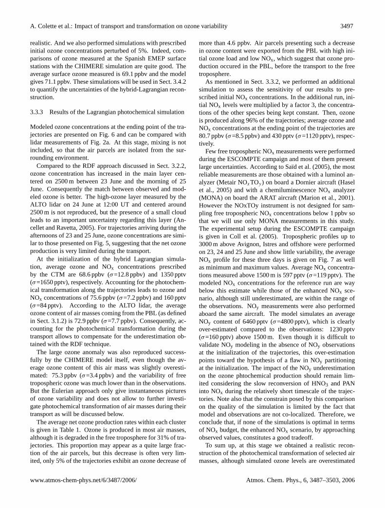
Few free tropospheric NOx measurements were performedduring the ESCOMPTE campaign and most of them presentlarge uncertainties. According to Saıd et al. (2005), the mostreliable measurements are those obtained with a luminol an-alyzer (Metair NOxTOy) on board a Dornier aircraft (Haselet al., 2005) and with a chemiluminescence NOx analyzer(MONA) on board the ARAT aircraft (Marion et al., 2001).However the NOxTOy instrument is not designed for sam-pling free tropospheric NOx concentrations below 1 ppbv sothat we will use only MONA measurements in this study.The experimental setup during the ESCOMPTE campaignis given in Coll et al. (2005). Tropospheric profiles up to3000 m above Avignon, Istres and offshore were performedon 23, 24 and 25 June and show little variability, the averageNOx profile for these three days is given on Fig. 7 as wellas minimum and maximum values. Average NOx concentra-tions measured above 1500 m is 597 pptv (σ=119 pptv). Themodeled NOx concentrations for the reference run are waybelow this estimate while those of the enhanced NOx sce-nario, although still underestimated, are within the range ofthe observations. NOy measurements were also performedaboard the same aircraft. The model simulates an averageNOy content of 6460 pptv (σ=4800 pptv), which is clearlyover-estimated compared to the observations: 1230 pptv(σ=160 pptv) above 1500 m. Even though it is difficult tovalidate NOy modeling in the absence of NOy observationsat the initialization of the trajectories, this over-estimationpoints toward the hypothesis of a flaw in NOy partitioningat the initialization. The impact of the NOy underestimationon the ozone phtochemical production should remain lim-ited considering the slow reconversion of HNO3 and PANinto NOx during the relatively short timescale of the trajec-tories. Note also that the constrain posed by this comparisonon the quality of the simulation is limited by the fact thatmodel and observations are not co-localized. Therefore, weconclude that, if none of the simulations is optimal in termsof NOx budget, the enhanced NOx scenario, by approachingobserved values, constitutes a good tradeoff.

To sum up, at this stage we obtained a realistic recon-struction of the photochemical transformation of selected airmasses, although simulated ozone levels are overestimated



0 1000 20000

500

1000

1500

2000

2500

3000Al

titud

e (m

)

NOx (pptv)

Fig. 7. NOx profiling with the MONA instrument on board theARAT aircraft in the ESCOMPTE region. The average profile forthe flights of the 23rd, 24th, and 25th of June is given (bold) as wellas minimum and maximum values.

compared to lidar measurements. Consequently, we decidedto account for the mixing with background air to achieve abetter comparison with the observations.

3.4 Impact of the mixing along the trajectories

For both the reference run and the “enhanced NOx” scenario,the hybrid-Lagrangian model overestimates ozone concen-trations. The fact that air parcels are isolated from the sur-rounding environment plays a role in this overestimation(Wild et al., 1996) and justifies the need to account for themixing with background air.

3.4.1 Methodology

In this study, we chose to mix air parcels with a climatolog-ical background. The species concerned by this mixing are:O3, H2O2, NO, NO2, HONO, HNO3, CO, SO2, CH4, C2H6,C4H10, C2H4, C3H6 and PAN. A test case where mixing waslimited to ozone showed that the impact of mixing of theother constituents was limited. The strength of the mixing ischaracterized by a characteristic time, i.e. the e-folding timenecessary to reach background concentrations if the compo-sition of air parcels were exclusively subject to the mixing.

The relaxation field is a climatology corresponding to thethree-dimensional average of CHIMERE outputs between 15June and 25 June. The average free tropospheric ozone con-centration along trajectories coming from the Spanish PBL is64.7 ppbv (σ=7.8 ppbv) which is in the range of the climatol-ogy based on balloon soundings proposed by Logan (1999).The purpose of this parameterization of the mixing is to ac-count for the interactions with background air. That is whythe relaxation field is climatological. Mixing with time de-pendant 3-D CHIMERE outputs would make sense if onewould expect that the trajectory encountered an Europeanpolluted plume that was simulated by CHIMERE, while theMesoNH model would have missed the mixing of air masseswith distinct origins. However, considering the resolution ofthe semi-Lagrangian trajectories, such an event would havebeen detected in the analysis of transport processes.

The mean and standard deviation of modeled ozone distri-butions as well as average NOx concentrations are given onFig. 8 for characteristic mixing times between half a day and7 days. Results of the no-mixing runs and measured ozoneand NOx concentrations are also given.

3.4.2 Results

Modeled and observed standard deviations of ozone aregiven on Fig. 8c. Figure 8d displays the Fisher test used forcomparing the standard deviation of two populations whentheir mean is not known and the 95% confidence level (Bev-ington and Robinson, 1992). The reference is the ALTOrecord. The standard deviation of ozone distributions in CiT-TyCAT outputs decreases with the characteristic mixing timesince concentrations are relaxed toward a climatological 3-Dfield. Increasing initial NOx concentrations tend to producemore ozone in air masses where NOx levels were already sig-nificant. Consequently, standard deviations for these high-NOx simulations are higher. For the enhanced NOx scenario,the mixing time should not be faster than about 2.5 days forthe standard deviation of ozone to remain statistically similarto that measured by the lidar. For the reference simulation,the modeled and measured standard deviations become sim-ilar if the mixing time is larger than 5.5 days.

Average ozone concentrations are displayed on Fig. 8a.The Student t-test and its 95% confidence level are givenon Fig. 8b, the reference being the ALTO estimate. Again,we find that average ozone concentrations are overestimatedfor no-mixing CiTTyCAT runs. Accounting for the mixingmakes average ozone more realistic. Nonetheless for the en-hanced NOx scenario, it is not statistically similar to mea-sured ozone concentrations if mixing time differs from 1.5 to2.5 days. For the reference run, mixing times included in the3 to 7 days range give satisfactory results.

To sum up, the optimum between average and standarddeviation of modeled ozone is reached for a characteristicmixing time of 6 and 2.5 days depending on the initial NOxconcentrations considered. As mentioned above, important



0 1 2 3 4 5 6 7 no mix0.5

1

1.5

2

2.5Fisher test on standard deviation

0 1 2 3 4 5 6 7 no mix

4

6

8

Standard deviation of ozone concentrations (ppbv)

0 1 2 3 4 5 6 7 no mix

−10

0

10

Student T−test on average ozone

0 1 2 3 4 5 6 7 no mix606570758085

Average ozone concentration (ppbv)

0 1 2 3 4 5 6 7 no mix0

200

400

600Average NOx concentration (pptv)

Characteristic time of turbulent mixing (days)

Fig. 8. Average and standard deviation of ozone concentrations(a, c) and average NOx (e) modeled with the hybrid-Lagrangian modelfor different characteristic time of turbulent mixing. For the reference run (blue) and the enhanced initial NOx scenario (red). Results ofno-mixing simulations are also displayed as well as observations (black, ALTO for ozone and MONA for NOx). Panels(b) and(d) presentstatistical tests for the validity of the comparison with the ALTO record with 95% confidence levels (dashed). The shaded areas correspondto optimum mixing times for the reference (blue), the enhanced NOx simulations (red), or both (violet).

uncertainties exist regarding the NOx levels at the initializa-tion of the trajectories. For all the scenarios investigated,modeled NOx concentrations are below the average mea-sured NOx concentrations (Fig. 8e). Nonetheless, results aremuch more realistic in the enhanced NOx cases than in thereference runs.

Now that we have identified the best simulations, we willbe able to quantify ozone production efficiency during thetransport in the free troposphere. Before proceeding to thisanalysis, we must assess uncertainties on mixing time dis-cussed here above. First, as we mentioned in Sect. 3.3.2,simulations with a 5% change in initial ozone concentrationswere performed. These simulations yield to a 2.5 ppbv dif-ference at the ending point of the trajectory for the enhanced

NOx scenario. According to Fig. 8a, this difference corre-sponds to an uncertainty smaller than 1 day on the character-istic mixing time. Second, a 5% change in the ozone clima-tological background leads to a 0.2 day change in the charac-teristic mixing time (because the relaxation toward the clima-tological field follows an exponential law). We can thus con-clude that the uncertainty on the characteristic mixing time isabout 1 day.

3.5 Ozone production efficiency

Net ozone production (P(O3)) along the trajectories can beinferred from photochemical ozone production and loss dur-ing the transport as modeled by CiTTyCAT. For the referencesimulation the optimum mixing time is 6 days (Sect. 3.4.2).



With this value, we find an average ozone production rate of0.09 ppbv h−1 (σ=0.12 ppbv h−1). However, if ozone con-centrations are satisfactory in the reference run, NOx lev-els are underestimated. Consequently, the average produc-tion rate of 0.19 ppbv h−1 (σ=0.11 ppbv h−1) obtained witha mixing time of 2.5 days in the enhanced NOx scenario isprobably a better estimate.

Production rates in the clusters of trajectories are given onTable 1 for both simulations. The clusters behave similarlywhen increasing initial NOx concentration, i.e. P(O3) in-creases in every cluster. One exception is found for cluster 23because (1) its initial NOx is already very high (Fig. 5b), al-lowing to switch to a NOx saturated regime as described inSillman (1999) and (2) this cluster is of little significancewith only 5 trajectories (Table 1). For some clusters, pro-duction rates stand out of the distribution, i.e. are greater orsmaller than the average plus or minus one standard devia-tion. In clusters 3, 4, 5 and 6, production is very high (about0.4 ppbv h−1 for the enhanced NOx scenario). Trajectoriesbelonging to these clusters were exported toward the FT inthe morning with high initial NOx and moderate ozone con-centrations, paving the way for high ozone production dur-ing free tropospheric transport. Such ozone production lev-els are comparable to those found by Evans et al. (2000) andMethven et al. (2003) for polluted air masses associated torecent export from the PBL. Low production rates (net de-struction of ozone) are found in clusters 12 and 18. Thesetrajectories were exported from the PBL in areas of low emis-sions according to CHIMERE (around Salamanca and Northof Granada).

On average for all the trajectories, the initial ozoneconcentration when air masses left the Iberian PBL was68.6 ppbv (σ=12.8 ppbv). The final average concentrationabove the ESCOMPTE area is 74.7 ppbv (σ=5.8 ppbv) ac-cording to the enhanced NOx run with a 2.5 day mixing time.Consequently, 6.1 ppbv of ozone are produced in the free tro-posphere. If the tropospheric ozone burden for this periodis approximated as the average ozone concentrations mea-sured by lidar above 2000 m, we find a background level of61.4 ppbv. We can thus conclude that PBL venting is respon-sible for an increase of 13.3 ppbv of free tropospheric ozoneconcentrations, about 45% of this increase being related tophotochemical production during the transport. Accountingfor the 1 day uncertainty on the optimum mixing time dis-cussed above, we find the contribution of free troposphericproduction of the order of 30% to 50% (38 to 45% for thereference run). Using a global CTM, Liang et al. (1998)found that, on an annual basis, ozone production in the freetroposphere is twice as large as direct export for the Ameri-can PBL. The comparison of our approach (small scale, andlimited to the ESCOMPTE period and location) to an annualestimate with a global model can only be used to put ourresults in a broader perspective. But both approaches leadto highlighting the need to account for ozone photochemicalproduction during the transport in the free troposphere.

4 Conclusion

The free tropospheric ozone variability observed by lidar dur-ing the ESCOMPTE campaign was investigated by means ofa hybrid-Lagrangian modeling study. The purpose of thiswork was to document the respective impact of transport andtransformation on the observed free tropospheric ozone vari-ability.

High-resolution backtrajectories were computed using amesoscale model including semi-Lagrangian tracking of airparcels. Ozone-rich layers are related to air masses extractedrecently from the Iberian PBL. A similar synoptic situationwas discussed by Millan et al. (1997) who reports that ex-port from the Iberian PBL occurs through local scale circu-lations (sea-breezes and orographic winds or a combinationof both) or convective activity. The chemical composition ofair masses when they left the PBL was inferred from CTMsimulations. Comparison with the observations shows thatphotochemical transformation in the troposphere can not beneglected.

This transformation was modeled using a Lagrangianchemistry model which allowed simulating successfully thelarge ozone rich anomalies measured by lidar. One of the re-markable features is the fact that the shape and the ozone con-tent of the large ozone-rich layer measured between the after-noon of 23 June and the morning of 25 June are well repro-duced. We found that this event was constituted of air massescoming from widespread locations above Spain and their ini-tial trace gases composition showed a high variability. Nev-ertheless, when these air masses reach the ESCOMPTE areathey appear (according to both the measurement and the La-grangian reconstruction) as a single layer with relatively ho-mogeneous ozone content.

Different scenarios regarding initial NOx concentrationswere investigated to achieve a satisfactory comparison withozone and NOx measurements performed during the ES-COMPTE campaign. Modeled ozone concentrations areoverestimated if mixing with background air is neglected.The optimum simulations are found for a characteristic mix-ing time of the order of 6 and 2.5 days for the reference runand the enhanced NOx scenario (initial NOx levels multipliedby a factor 3), respectively. The uncertainty regarding thesemixing times is about 1 day.

According to the simulation based on the optimum mixingtime, ozone is produced during the transport for the major-ity of air masses. Ozone production efficiency is highest forair masses that left the PBL in the morning (0.4 ppbv h−1),i.e. before photochemical transformation began in the PBL.On average, ozone production rate during the transport is ofthe order of 0.2 ppbv h−1; that is an 13.3 ppbv increase dur-ing the transport in the free troposphere.

We found that the contribution of ozone produced in thefree troposphere is at most as important as direct export ofozone in the PBL. These two processes are responsible forabout 45% and 55% of the ozone increase related to PBL



venting, respectively. During this event, we sampled airmasses coming from widespread locations above Spain andat different times of the day. We can thus conclude that theSpanish PBL was a net exporter of ozone and of its precur-sors to the free troposphere during that period.

Acknowledgements.We thank all the participants to the ES-COMPTE campaign that contributed to the gathering of animpressive dataset, and especially P. Perros for NOx measurmentsand the EPFL team for ozone lidar profiling. The MesoNHteam is gratefully acknowledged for assistance with the code(F. Gheusi, J. Escobar). R. Vautard provided MM5 simulationsto drive CHIMERE simulations. Inputs for the CHIMERE modelwere provided by EMEP (yearly totals), IER (time variations),TNO (aerosol emissions), and UK Department of Environment(VOC speciation). A. Stohl gave helpful advices regarding theFLEXPART model. E. Real is also acknowledged for assistanceregarding CiTTyCAT. EUMETSAT granted access to satelliteimagery. Meteorological analyses were provided by ECMWF. Thiswork was funded in part by Total (C. Puel and O. Duclaux).

Edited by: H. Wernli

References

Ancellet, G. and Ravetta, F.: A compact airborne lidar for tro-pospheric ozone (ALTO): description and field measurements,Appl. Opt., 37, 5509–5521, 1998.

Ancellet, G. and Ravetta, F.: Analysis and validation of ozonevariability observed by lidar during the ESCOMPTE-2001 cam-paign, Atmos. Res., 74, 435–459, 2005.

Bastin, S. and Drobinski, P.: Sea breeze induced mass transport overcomplex terrain in southeastern France: A case study, Quart. J.Roy. Met. Soc., 132, 405–423, 2006.

Bastin, S., Drobinski, P., Dabas, A., Delville, P., Reitebuch O., andWerner, C.: Impact of the Rhone and Durance valleys on sea-breeze circulation in the Marseille area, Atmos. Res., 74, 303–328, 2005.

Bernsten, T. K., Isaksen, I. S. A., Myhre, G., Fuglestvedt, J. S.,Stordal, F., Larsen, T. A., Freckleton, R. S., and Shine, K. P.:Effects of anthropogenic emissions on tropospheric ozone and itsradiative forcing, J. Geophys. Res., 102, 28 101–28 126, 1997.

Bevington, P. R. and Robinson, D. K.: Data reduction and erroranalysis for the physical sciences, 2nd edition, McGraw-HillBook Co, New York, USA, 328 p., 1992.

Coll I., Pinceloup, S., Perros, P. E., Laverdet, G., and Le Bras, G.:3D analysis of the High Ozone Production Rates observed duringthe ESCOMPTE campaign, J. Atmos. Res., 74, 477–505, 2005.

Cooper, O. R., Moody, J. L., Parrish, D. D., Trainer, M., Ryerson,T. B., Holloway, J. S., Hubler, G., Fehsenfel, F. C., and Evans,M. J.: Trace gas composition of midlatitude cyclones over thewestern North Atlantic Ocean: A conceptual model, J. Geophys.Res., 107(D7), doi:10.1029/2001JD000901, 2002.

Corsmeier, U., Behrendt, R., Drobinski P., and Kottmeier, C.: Themistral and its effect on air pollution transport and vertical mix-ing, Atmos. Res., 74, 275–302, 2005.

Cotton, W. R., Alexander, G. D., Hertenstein, R., Walko, R. L.,McAnelly, R. L., and Nicholls, M.: Cloud venting, A review

and some new global annual estimates, Earth-Sci. Rev., 39(3–4),169–206, 1995.

Cousin, F., Tulet, P., and Rosset, R.: Interaction between local andregional pollution during ESCOMPTE 2001: impact on surfaceozone concentrations (IOP2a and 2b), Atmos. Res., 74, 117–137,2005.

Cros, B. and Durand, P.: Preface, Guest editors, Atmos. Res., 74(1–4), 2005.

Cros, B., Durand, P., Cachier, H., Drobinski, P., Frejafon, E.,Kottmeier, C., Perros, P. E., Peuch, V.-H., Ponche, J.-L., Robin,D., et al.: The ESCOMPTE program: an overview, Atmos. Res.,69, 241–279, 2004.

Dufour, A., Amodei, M., Ancellet, G., and Peuch, V.-H.: Observedand modelled “chemical weather” during ESCOMPTE, Atmos.Res., 74, 161–189, 2005.

Eckhardt, S., Stohl, A., Beirle, S., Spichtinger, N., James, P.,Forster, C., Junker, C., Wagner, T., Platt, U., and Jennings, S.G.: The North Atlantic Oscillation controls air pollution trans-port to the Arctic, Atmos. Chem. Phys., 3, 1769–1778, 2003,http://www.atmos-chem-phys.net/3/1769/2003/.

ECMWF: User Guide to ECMWF Products 2.1, MeteorologicalBulletin M3.2, ECMWF, Reading, UK, 49 p., 1995.

Evans, M. J., Shallcross, D. E., Law, K. S., Wild, J. O. F., Sim-monds, P. G., Spain, T. G., Berrisford, P., Methven, J., Lewis,A. C., McQuaid, J. B., Pillinge, M. J., Bandyf, B. J., Penkettf,S. A., and Pyle, J. A.: Evaluation of a Lagrangian box modelusing field measurements from EASE (Eastern Atlantic SummerExperiment) 1996, Atmos. Environ., 34(23), 3843–3863, 2000.

Gangoiti, G., Millan, M. M., Salvador, R., and Mantilla, E.: Long-range transport and re-circulation of pollutants in the westernMediterranean during the project Regional Cycles of Air Pollu-tion in the West-Central Mediterranean Area, Atmos. Environ.,35(36), 6267–6276, 2001.

GENEMIS: Generation of European Emission Data for Episodesproject, EUROTRAC annual report 1993, part 5, EUROTRACinternational scientific secretariat, Garmisch-Partenkirchen, Ger-many, 1994.

Gheusi, F. and Stein, J.: Lagrangian description of airflows usingEulerian passive tracers, Quart. J. Roy. Met. Soc., 128, 337–360,2002.

Gheusi, F., Cammas, J. -P., Cousin, F., Mari, C., and Mascart, P.:Quantification of mesoscale transport across the boundaries ofthe free troposphere: a new method and applications to ozone,Atmos. Chem. Phys. Discuss., 4, 8103–8139, 2004,http://www.atmos-chem-phys-discuss.net/4/8103/2004/.

Good, P., Giannakopoulos, C., O’Connor, F. M., Arnold, S. R., deReus, M., and Schlager, H.: Constraining tropospheric mixingtimescales using airborne observations and numerical models,Atmos. Chem. Phys., 3, 1023–1035, 2003,http://www.atmos-chem-phys.net/3/1023/2003/.

Hasel, M., Kottmeier, C., Corsmeier, U., and Wieser, A.: Airbornemeasurements of turbulent trace gas fluxes and analysis of eddystructure in the convective boundary layer over complex terrain,Atmos. Res., 74, 381–402, 2005.

Hauf, T., Schulte, P., Alheit, R., and Schlager, H.: Rapid verticaltrace gas transport by an isolated midlatitude thunderstorm, J.Geophys. Res., 100(D11), 22 957–22 970, 1995.

Hauglustaine, D. A., Hourdin, F., Jourdain, L., Filiberti, M.-A., Walters, S., Lamarque, J.-F., and Holland, E. A.: In-


http://www.atmos-chem-phys.net/3/1769/2003/

http://www.atmos-chem-phys-discuss.net/4/8103/2004/



teractive chemistry in the Laboratoire de Meteorologie Dy-namique general circulation model: Description and back-ground tropospheric chemistry evaluation, J. Geophys. Res., 109,doi:10.1029/2003JD003957, 2004.

Henne, S., Furger, M., Nyeki, S., Steinbacher, M., Neininger, B.,deWekker, S. F. J., Dommen, J., Spichtinger, N., Stohl, A., andPrevot, A. S. H.: Quantification of topographic venting of bound-ary layer air to the free troposphere, Atmos. Chem. Phys., 4, 497–509, 2004,http://www.atmos-chem-phys.net/4/497/2004/.

Kalthoff, N., Kottmeier, C., Thurauf, J., Corsmeier, U., Saıd, F.,Frejafon, E., and Perros, P. E.: Mesoscale circulation systemsand ozone concentrations during ESCOMPTE: a case study fromIOP 2b, Atmos. Res., 74, 355–380, 2005.

Kleinman, L. I., Daum, P. H., Lee, J. H., Lee, Y.-N., Nunnerma-cker, L. J., Springston, S. R., Newman, L., Weinstein-Lloyd, J.,and Sillman, S., Dependence of ozone production on NO andhydrocarbons in the troposphere, Geophys. Res. Lett., 24(18),2299–2302, doi:10.1029/97GL02279, 1997.

Konovalov, I. B., Beekmann, M., Vautard, R., Burrows, J. P.,Richter, A., Nuß, H., and Elansky, N.: Comparison and evalua-tion of modelled and GOME measurement derived troposphericNO2 columns over Western and Eastern Europe, Atmos. Chem.Phys., 5, 169–190, 2005,http://www.atmos-chem-phys.net/5/169/2005/.

Lafore, J.-P., Stein, J., Asencio, N., Bougeault, P., Ducrocq, V.,Duron, J., Fischer, C., Hereil, P., Mascart, P., Masson, V., Pinty,J.-P., Redelsperger, J.-L., Richard, E., and Vila-Guerau de Arel-lano, J.: The Meso-NH Atmospheric Simulation System. Part I:adiabatic formulation and control simulations. Scientific objec-tives and experimental design, Ann. Geophys., 16, 90–109, 1998,http://www.ann-geophys.net/16/90/1998/.

Lattuati, M.: Contributiona l’etude du bilan de l’ozone tro-pospheriquea l’interface de l’Europe et de l’Atlantique Nord:Modelisation lagrangienne et mesures en altitude, Ph.D. Thesis,Universite Paris 6, Paris, 1997.

Lawrence, M. G., Von Kuhlmann, R., Salzmann, M., andRasch, P. J.: The balance of effects of deep convectivemixing on tropospheric ozone, Geophys. Res. Lett., 30(18),doi:10.1029/2003GL017644, 2003.

Lelieveld, J., Berresheim, H., Borrmann, S., Crutzen, P. J., Den-tener, F. J., Fischer, H., Feichter, J., Flatau, P. J., Heland,J., Holzinger, R., Korrmann, R., Lawrence, M. G., Levin, Z.,Markowicz, K. M., Mihalopoulos, N., Minikin, A., Ramanathan,V., de Reus, M., Roelofs, G. J., Scheeren, H. A., Sciare, J.,Schlager, H., Schultz, M., Siegmund, P., Steil, B., Stephanou,E. G., Stier, P., Traub, M., Warneke, C., Williams, J., and Ziereis,H.: Global Air Pollution Crossroads over the Mediterranean, Sci-ence, 298(5594), 794–799, 2002.

Liang, J., Horowitz, L. W., Jacob, D. J., Wang, Y., Fiore, A. M., Lo-gan, J. A., Gardner, G. M., and Munger, J. W.: Seasonal budgetsof reactive nitrogen species and ozone over the United States,and export fluxes to the global atmosphere, J. Geophys. Res.,103(D11), doi:10.1029/97JD03126, 1998.

Logan, J. A.: An analysis of ozonesonde data for the troposphere:Recommendations for testing 3-D models and development ofa gridded climatology for tropospheric ozone, J. Geophys. Res.,104(D13), doi:10.1029/1998JD100096, 1999.

MacQueen, J.: Some methods for classification and analysis multi-

variate observations, 5th Berkeley Symposium of MathematicalStatistics and Probability 1, 281–297, 1967.

Marion, T., Perros, P. E., Losno, R., and Steiner, E.: OzoneProduction Efficiency in Savanna and Forested Areas dur-ing the EXPRESSO Experiment, J. Atmos. Chem., 38(1),doi:10.1023/A:1026585603100, 2001.

Methven, J., Evans, M., Simmonds, P., and Spain, G.: Estimatingrelationships between air mass origin and chemical composition,J. Geophys. Res., 106(D5), 5005–5020, 2001.

Methven, J., Arnold, S. R., O’Connor, F. M., Barjat, H., Dewey, K.,Kent, J., and Brough, N.: Estimating photochemically producedozone throughout a domain using flight data and a Lagrangianmodel, J. Geophys. Res., 108(D9), doi:10.1029/2002JD002955,2003.

Mill an, M. M., Salvador, R., Mantilla, E., and Kallos, G.: Photoox-idant dynamics in the Mediterranean basin in summer: Resultsfrom European research projects, J. Geophys. Res., 102(D7),doi:10.1029/96JD03610, 1997.

Norton, W. A.: Breaking Rossby Waves in a Model Stratosphere Di-agnosed by a Vortex-Following Coordinate System and a Tech-nique for Advecting Material Contours, J. Atmos. Sci., 51, 654–673, 1994.

Parrish, D. D., Ryerson, T. B., Holloway, J. S., Neuman, J. A.,Roberts, J. M., Williams, J., Stroud, C. A., Frost, G. J., Trainer,M., Hubler, G., Fehsenfeld, F. C., Flocke, F., and Weinheimer, A.J.: Fraction and composition of NOy transported in air masseslofted from the North American continental boundary layer, J.Geophys. Res., 109, D09302, doi:10.1029/2003JD004226, 2004.

Puygrenier, V., Lohou, F., Campistron, B., Saıd, F., Pigeon, G.,Benech, B., and Serca, D.: Investigation on the fine structureof sea-breeze during ESCOMPTE experiment, Atmos. Res., 74,329–353, 2005.

Reeves, C. E., Penkett, S. A., Bauguitte, S., Law, K. S., Evans, M. J.,Bandy, B. J., Monks, P. S., Edwards, G. D., Phillips, G., Barjat,H., Kent, J., Dewey, K., Schmitgen, S., and Kley, D.: Potentialfor photochemical ozone formation in the troposphere over theNorth Atlantic as derived from aircraft observations during AC-SOE, J. Geophys. Res., 107(D23), doi:10.1029/2002JD002415,2002.

Saıd, F., Corsmeier, U., Kalthoff, N., Kottmeier, C., Lothon, M.,Wieser, A., Hofherr, T., and Perros, P. E.: ESCOMPTE exper-iment: intercomparison of four aircraft dynamical, thermody-namical, radiation and chemical measurements, Atmos. Res., 74,217–252, 2005.

Schmidt, H., Derognat, C., Vautard, R., and Beekmann, M.: A com-parison of simulated and observed ozone mixing ratios for thesummer of 1998 in Western Europe, Atmos. Environ., 35(36),6277–6297, 2001.

Sillman, S.: The relation between ozone, NOx and hydrocarbons inurban and polluted rural environments, Atmos. Env., 33, 1821–1845, 1999.

Simeonov, P., Ristori, P., Balin, I., Calpini, B., and van den Bergh,H.: A new DIAL based on a N2 Raman converter for ozone mon-itoring; design and application during the ESCOMPTE Cam-paign, Proc. of the XX Quaternary Ozone Symposium, Greece,109–110, 2004.

Stohl, A. and Trickl, T.: A textbook example of long-rangetransport: Simultaneous observation of ozone maxima ofstratospheric and North American origin in the free tropo-




http://www.ann-geophys.net/16/90/1998/


sphere over Europe, J. Geophys. Res., 104, 30445–30462,10.1029/1999JD900803, 1999.

Stohl, A., Hittenberger, M., and Wotawa, G.: Validation of theLagrangian particle dispersion model FLEXPART against largescale tracer experiment data, Atmos. Environ., 32(24), 4245–4264, 1998.

Stohl, A., Forster, C., Frank, A., Seibert, P., and Wotawa, G.: Tech-nical note: The Lagrangian particle dispersion model FLEX-PART version 6.2, Atmos. Chem. Phys., 5, 2461–2474, 2005,http://www.atmos-chem-phys.net/5/2461/2005/.

Vautard, R., Beekmann, M., Roux, J., and Gombert, D.: Validationof a hybrid forecasting system for the ozone concentrations overthe Paris area, Atmos. Environ., 35(14), 2449–2461, 2001.

Vautard, R., Honore, C., Beekmann, M., and Rouil, L.: Simulationof ozone during the August 2003 heat wave and emission controlscenarios, Atmos. Environ., 39(16), 2957–2967, 2005.

Wild, O., Law, K. S., McKenna, D. S., Bandy, B. J., Penkett, S. A.,and Pyle, J. A.: Photochemical trajectory modeling studies ofthe North Atlantic region during August 1993, J. Geophys. Res.,101, 29 269–29 288, 1996.

Zhang, J. and Trivikrama Rao, S.: The Role of Vertical Mixing inthe Temporal Evolution of Ground-Level Ozone Concentrations,J. Appl. Met., 38, 1674–1691, 1999.



a lagrangian analysis of the impact of transport and

Documents