A LABORATORY MANUAL

FOR

ELECTRICAL ENGINEERING 201.3

REVISED 2007

Department of Physics & Engineering Physics

University of Saskatchewan

E.E. 201.3 Laboratory Manual

TABLE OF CONTENTS

INTRODUCTION Page A: General Instructions ......................................................................... i B: Laboratory Reports .......................................................................... iii C: Graphical Representation and Interpretation of Experimental Data ....................................................................... vii D: Discussion of Errors ......................................................................... xv E: Significant Figures ........................................................................... xvii F: Estimating Absolute Errors from Random Causes .......................... xix G: Propagation of Errors in Calculations .............................................. xxi H: Sample Calculations ......................................................................... xxix I: Comparing Two Quantities .............................................................. xxx

Experiment

E30 A. AC Measurements of Capacitance & Inductance ........................................ 1

B. Phase Measurements in AC Circuits ............................................................ 3

E31 Phasor Analysis .................................................................................................. 8

E36 The Electric Current Balance ............................................................................. 16

E50 Electromagnetic Induction: Faraday’s and Lenz’s Laws .................................. 21

E52 Magnetic Circuits ............................................................................................... 27

E55 DC Response of RC, LR, and LCR Circuits …………..………………………. 34

i

A: GENERAL INSTRUCTIONS

Safety in the Laboratory

The safety issues related to the equipment and procedures used in the Electrical Engineering 201 laboratory are as follows:

thermal hazards due to high current in rheostat (experiment E36) electrical hazards, including potentially high current and ac line voltage (all experiments)

General Safety Policies

No food or drink is to be consumed in the laboratory Liquids brought into the lab room must be kept in sealed containers, which are not to be opened in the lab room and which must be placed on the floor (i.e. below the lab bench).

Follow all instructions In addition to the instructions in the laboratory manual, follow all verbal and written instructions provided by the instructional staff.

Come Prepared to the Laboratory

A proper understanding of your physics class requires a combination of studying the lecture material, solving problems, and performing experiments in the laboratory. An attempt has been made to relate the experimental work directly to the lecture material. Due to space and equipment limitations, however, experimental work may, in some cases, have to be carried out before the topic has been covered in the lectures. To compensate for this, before coming to the laboratory you should carefully read the sections of your text which are covered in the assigned experiment. If the material has been taken in lectures, the lecture notes should be studied as well. After having done this preparatory reading, carefully review the object, theory and procedure outlined in the lab manual so that you have an understanding of the purpose of the experiment, what data will be required to accomplish that purpose, and how that data will be collected. Use the material presented in this manual to plan in advance the way the experimental work should be organized.

Partners

Students will work in pairs (or groups of 3 if necessary) but each student is expected to prepare her or his own account of the work. This does not imply that partners should not cooperate; time and effort can be saved by working together in sharing the numerical calculations, checking results, and discussing the theory and performance of each experiment. Partners should share the work so that both partners understand the whole of the experiment and become familiar with the equipment. If your performance could be improved by exchanging partners, please request the demonstrator in your laboratory to arrange this, if possible.

Laboratory Schedule

A schedule of experiments will be posted in display cases near the laboratory. Each experiment normally occupies one morning or afternoon. Limited provision will be made in the schedule for the performance of those experiments which, for a legitimate reason, are not carried out at the regularly scheduled time.

ii

Grades

Each instructor will explain the arrangements for submitting the reports, and for returning the marked reports. Each student is responsible for submitting on time a complete account of each of her/his experiments. Laboratory reports are marked by the student assistants. Note that all the assigned experiments must be completed to obtain credit in the course.

Materials

Each student should bring to the laboratory a physics laboratory notebook (coil-bound with ¼" grid paper), an inexpensive set of geometrical instruments and a calculator with trigonometric functions. Specific instructions about the materials required for the laboratory will be given in the first meeting of the class.

Absenteeism

Students who are absent from a laboratory period may be allowed to arrange with the laboratory instructor to perform the experiment some other time. If there are extenuating circumstances, such as ill health, etc., this should be discussed with the demonstrator as soon as possible.

Assistance in the Laboratory

The demonstrator in the laboratory is there to assist you. When something arises which you do not understand, and which cannot be resolved with the help of your partner, please consult the demonstrator.

Before leaving the laboratory, return equipment to its original location so that the next group will not start their experiment at a disadvantage. Disconnect electrical connections and return the connecting wires to the cupboards. Turn off any gas, water, or air sources that were used during the experiment.

iii

B: LABORATORY REPORTS

One of the aims of this laboratory is to teach you the methods that professional physicists have found satisfactory for recording the performance of experiments. Two criteria should be met by a satisfactory laboratory report:

1. A person with an educational background similar to yours should be able to easily follow through the experiment by reading your report, and if desired should be able to easily perform the experiment, obtaining results similar to yours.

2. The results of your study should stand out clearly and the conclusions drawn from these results should follow logically.

A suggested approach follows on the organization of your work to meet the above criteria. Details, such as correct procedures for drawing graphs, calculating errors, etc. are covered in later sections.

A log book format, rather than a formal lab report format will be used. The emphasis is on whether or not you understood and properly performed the experiment. The information contained in the log book should clearly indicate how the experiment was performed, what measurements were made, how these measurements were analyzed, and what conclusions were drawn. It is essential that you read the laboratory manual before coming to the lab so that you have a basic understanding of what you will be doing. The report for each experiment will contain the following sections:

Heading title of experiment, date experiment performed, your name, partner's name overall format of report worth ½ mark

Object one or two sentences describing purpose of experiment worth ½ mark

Experiment Data Collection diagram of equipment, notes outlining procedure steps, and data, for each part of the

experiment a brief procedure note should accompany the equipment diagram, e.g. “The spark timer is

used to record a trace of the position of the cart at equally spaced time intervals.” This note can be written before you come to the laboratory, all other procedure notes are to be done at the time the measurements are made and are to be very brief. If the result of a particular step in the procedure is the measurement of a single quantity, the procedure note can be incorporated in the recording of the measurement. For example, “distance between legs of air track, measured with tape measure: L = 153.2 ± 0.4 cm” would be a suitable procedure note. If a number of measurements are made by repetition of a single procedure, the procedure note forms a description of the corresponding table of values, e.g. “A ruler was used to measure the displacement, x, of the cart in 0.200 s time intervals at various points along the spark trace.”

data should be tabulated whenever possible

iv

tables must be titled, and as much information as possible is to be put in the column headings rather than included with each entry. The heading of a column contains a one- or two-word descriptive label, the symbol for the quantity being tabulated, the units, the power of ten if scientific notation is being used, and the experimental error (if constant for all values in column). Individual column entries will be numbers or numbers ± errors. See Table 1 further in this introduction for an example of a proper table.

data must be recorded, with their errors and units, directly into the lab notebook (transfer of measurements recorded on scrap paper wastes time and can introduce mistakes)

incorrect data are to be neatly crossed out with a single line in such a way that they are still legible

worth 3 marks

Analysis this section involves manipulation of the raw observational data by graphing, making

numerical calculations, or in some other way specified in the instructions sample calculation and error calculation for each different equation units must be carried through calculations use a separate, complete page for each graph analysis results should be presented in tabular form whenever possible if possible, compare experimental results with theoretical or accepted values. The primary

criterion to be used when comparing values is whether or not the values agree within experimental error (i.e. do the error ranges overlap?). Although it is not the preferred comparison criterion, percentage difference between experimental and accepted/theoretical values may be used on occasion.

worth 3 marks marks are lost in ½ mark increments for the following: calculation errors graph format errors units not carried through calculations poor presentation of results

Conclusion state results (with experimental error) and state whether or not there is agreement within

experimental error with theoretical or accepted values must include a discussion of the physical concepts examined in the experiment worth 2 marks

Sources of Error state as many factors as you can think of which might have affected the outcome of the

experiment, and which were not accounted for in any way explain how each of the above factors would be expected to affect your calculated results,

and whether the effects would be large or small random measuring error need not be mentioned (it is usually accounted for in error

calculations) the possibility of incorrectly calibrated measuring instruments should not be mentioned

unless there is a particular reason for doing so. The same holds for the possibility of incorrect calculations

v

worth 1 mark NOTE: BEFORE coming to the lab the Heading and Object should be written, the equipment

diagram should be drawn, and the Data Tables should be prepared.

Point-form may be used for the written sections of the report, but you must ensure that the meaning of your comments is clear.

At the discretion of the marker, a report may be worth an additional 1 mark (max. mark = 10). To receive this bonus mark the report must contain work in addition to that required by the manual. For example, provide constructive criticism and suggestions for improvement of the experiment or obtain additional data from which further conclusions relating to the experiment can be drawn.

NOTE: An average lab report is worth 7.0 marks. A good lab report is worth 8.0 marks. A very good lab report is worth 8.5 to 9.0 marks. An excellent lab report is worth 9.0 to 10 marks.

LOG BOOK STYLE SAMPLE The following is intended to show by example the style that is expected for your log book reports. 15 DEC 94 DETERMINATION OF GALVANOMETER BRIAN ZULKOSKEY FULL-SCALE DEFLECTION CURRENT

Object: to determine the current required to deflect the galvanometer needle to full-scale. Experiment: The following circuit was connected: Decade Resistance Box: R = 20,000 ± 1% The Current Control of the Heathkit Supply was set at maximum. The Voltage Control was initially set at minimum and was then slowly increased until the Galvanometer read full-scale (50) when button #3 was depressed. With the Galvanometer reading full-scale when button #3 was depressed: Heathkit Supply Voltage = 10.20 0.01 V

G

Heathkit Supply

decade resistor

galvanometer

vi

Analysis: Calculation of Full-scale Deflection Current (galvanometer resistance ignored):

IV

R 10 20

20 0005100 10 4.

,.

VA = 510.0 A

Error Calculation for Full-scale Deflection Current:

IV

RVR

I V R V R RV

RV

R

R

I

1

1 22 2

6

0 01

20 00010 20

200

20 000

5 6 10

|( )|.

,( . )

( , )

.

VV

A = 0.056 10 A = 5.6 A-4

The experimental value obtained for the galvanometer full-scale deflection current is 510.0 ± 5.6 A. Conclusion: The experimental value of 510.0 ± 5.6 A is reasonably close to the quoted nominal value of 500 A for the galvanometer full-scale deflection current. Using a simple circuit and Ohm’s Law enabled determination of one of the galvanometer parameters that must be known to use the galvanometer as a measuring instrument. Sources of Error: All of the errors in this procedure are expected to have small effects on the result. – if the galvanometer is not properly zeroed the measured full-scale current value will be too

large or too small depending on which side of 0 the needle initially lies (systematic error). – mechanical friction in the needle suspension may cause varying needle response (random

error). – judgement error in deciding when the meter is reading exactly full-scale (random error). – to account for possible variations in the meter response due to ‘direction of deflection’-

dependent mechanical properties, the full-scale deflection currents should have been measured for the meter deflecting to each side of 0, and the results averaged.

vii

C: GRAPHICAL REPRESENTATION AND INTERPRETATION OF EXPERIMENTAL DATA

In order to understand a physical problem, one usually studies the dependence of one quantity upon another. Whereas sometimes such a dependence is obtained theoretically, at times it must be arrived at experimentally. The experimental determination involves obtaining experimentally a series of values of one quantity corresponding to the various arbitrary values of the other and then subjecting the data to some kind of analysis. One of the most convenient and useful means of treating the experimental data is by graphical analysis.

A graph shows the relation between the two quantities in the form of a curve. Suppose we are interested in looking at the relation between the volume of a piece of iron and its mass. If we make measurements on pieces of iron, we find that 1 cm3 has a mass of 7.87 g, 2 cm3 has a mass of 15.74 g, 3 cm3 has a mass of 23.61 g, and so on. This kind of relation in which doubling the volume doubles the mass, tripling the volume triples the mass, is called direct proportion. In Physics you will encounter many cases of such relations. In describing this relation we say:

(i) mass ‘is directly proportional to’ volume of iron or mass ‘varies directly as’ the volume of iron.

(ii) Mathematically we can write the relation as M V, where M is the mass of a piece of iron and V is its volume and the symbol means ‘is proportional to’. If we have two different volumes of iron, V1 and V2, their masses M1 and M2 may be expressed as

2

1

2

1

V

V

M

M

Another form of this relation expresses the fact than when mass and volume are related by direct proportion, they have a constant ratio. Thus

V

M of one sample =

V

M of another sample = k

The constant k is called the proportionality constant. In our example of iron

k = 7.87 g for each cubic centimetre

We now express this relation as an equation for any piece of iron:

V

M = k or M = kV, where the value of k as determined experimentally is 7.87 g/cm3.

An equation established in this way is an empirical equation.

We can illustrate this relation between mass and volume for iron by a graph. In trying to study the mass of a piece of iron as a function of its volume, we chose certain values for the volume and determined the corresponding values for the mass. In such a situation volume is said to be the independent variable and the mass is the dependent variable. Generally, the independent variable should be the variable that is altered in regular steps in the experiment, and the dependent variable is the quantity which is measured for each regular step of the independent variable. The independent variable (in our case the volume of a piece of iron) is plotted along the x axis and the dependent variable (in our case, the mass of the piece of iron) is plotted along the y axis. To plot the data we must choose scales – one for the vertical direction, marking off some suitable number of grams for each vertical division of the paper, and one for the horizontal

viii

direction, marking off volumes in cm3. Now we can place a point on the graph for each pair of values that we know.

Volume, V (cm3)

Mass, M (g)

1 7.87

2 15.74

3 23.61

Note that a straight line can be drawn through the data points: the graph is linear. The ratio

V

M is the same for all points on the line, i.e. as already noted,

V

M = k or M = kV where k is

a constant. As seen here and discussed in the next section, M = kV is the equation of a straight line passing through the origin if M and V are plotted against each other. k is the slope of the line. General Linear Relationship

A straight line plot of y versus x indicates that the relationship is linear and is of the form

y = mx + b

where b is the intercept on the y-axis (the value of y when x = 0) and m is the slope of the line.

As an example, consider an examination of the relation between the strain (x) produced in a spring as a function of the applied force (F). A linear relation implies

F = kx + b

where k and b are constants. For this example refer to the data in Table 1.

Table 1: Spring Constant, Spring #1

Force, F (± 0.05N)

Average Strain, x (± 0.1 cm)

0.19 3.0 0.40 6.2 0.71 9.6 1.00 12.6 1.26 16.0 1.50 19.2

5

10

15

20

25

0 1 2 3

Volume (cm3)

Mas

s (g

)

ix

(x4, y4) = (19.2 cm, 1.55 N) (x2, y2) = (17.8 cm, 1.40 N)

N/m8.33N/cm0833.0

cm0.12

N00.1

cm8.5cm8.17

N40.0N40.1

slope12

12

xx

yy

N/m8.70N/cm0870.0

cm2.16

N41.1

cm0.3cm2.19

N14.0N55.1

slopemax34

34

xx

yy

(slope) = max slope – slope slope = 8.33 ± 0.37 N/m = 8.70 N/m – 8.33 N/m = 0.37 N/m (x1, y1) = (5.8 cm, 0.40 N) (x3, y3) = (3.0 cm, 0.14 N)

Average Strain, x (cm)

Graph 1: Force vs. Average Strain to determine Spring Constant

For

ce, F

(N

)

x

The experimentally obtained points usually do not lie exactly on a straight line; this is expected, because experimental data are never exact. In a straight line plot of experimental results, the straight line goes above some points and below others and represents an honest attempt on the part of the plotter to show the trend of the data. See Graph 1.

If the plot of y versus x yields a straight line, the relationship is linear and is of the form

y = mx + b

If m = 0, y does not depend on x. If the plot is a straight line passing through the origin, b = 0.

If the graph directly relating the variables does not give a straight line, one may search for the form of the function by considering a few of the common types of relationships one by one.

Power Relationship

One common type of relationship is of the form

u = cVn

where u and V are variables, c is a constant and n is the (constant) power to which V is raised and may be integral, fractional, positive, or negative. Taking logs of both sides gives

log u = log c + n log V

Letting log u = y, log c = b, and log V = x the equation becomes

y = nx + b

where both n and b are constants. The relationship can now be plotted as a straight line. A procedure of this type is called rectification of the data before plotting. In this case, instead of plotting u versus V, the rectified data, log u versus log V, is plotted. The slope of the line obtained will give the value of the exponent n. Such a plot is called a log-log plot and is a general method by which an exponent may be determined.

Figure 1: Rectification of a Power Relationship

xi

Consider Newton's Law of Gravitation (2r

MmGF ). As shown in Figure 1, the plot of F versus

r does not clearly show the functional relationship between F and r. An inspection of the plot of log F versus log r shows a slope of –2 and thereby indicates the inverse square relation.

Exponential Relationship

Some physical situations are described by an exponential relationship. Such relationships are most commonly written as powers of the number e (= 2.71828...), the base of natural logarithms.

Consider the general form of an exponential relationship: axceu where c and a are constants.

Taking logarithms to the base e (ln) of both sides of the equation gives

ln u = ln c + ax

Since c is a constant, ln c is also a constant, and therefore a plot of ln u versus x will be a straight line with slope a and y-intercept ln c. Such a plot is called a semi-log plot.

This type of relationship is illustrated by the following example:

The radioactive decay of a radioactive isotope is given by teNN 0

where N is the activity at time t, N0 is the initial activity at t = 0, and is the decay constant of the isotope. As shown in Figure 2, the plot of N versus t is curved but the semi-log plot, ln N versus t is linear, indicating that N varies exponentially with t.

Figure 2: Rectification of an Exponential Relationship

Other situations may arise where some thought is needed to devise a plot that will yield a straight line.

It is, however, not necessary to rectify the data to check the agreement of a theory with an experiment. A graph can be plotted of the results expected on the basis of theory as applied to the physical situation under study. The experimental points can be shown on the same graph. If the theory describes the situation adequately the experimental points will lie along the theoretical curve. If, however, the experimental data points do not follow the theoretical curve then either the proposed theory is inadequate or the experiment was not designed or performed properly.

xii

Special types of graph paper (log-log, semi-log) are available to quickly and easily test for and/or show power and exponential relationships. These papers are not marked in uniform squares. The distances along the axes are made proportional to the logarithms of the numbers that are shown on the axes. Calculators and computer plotting programs have replaced these special types of graph paper to a certain extent.

Figure 3 shows the data used in the graphs of Figure 1 (F vs. r) and Figure 2 (N vs. t) plotted on log-log and semi-log paper respectively.

The straight lines obtained indicate the power and exponential relationships respectively of these two sets of data. As discussed earlier, the slope of log F vs. log r is the value of the exponent in the power relationship. This can be determined from the log-log paper plot as follows:

210

02

)10log()1log(

)1log()100log(

loglog

loglogslopelog-log

12

12

rr

FF

Also as discussed earlier, the slope of ln N vs. t is the decay constant (the constant multiplying the variable in the exponent) of the exponential relationship. This can also be determined relatively easily from the semi-log paper plot.

decay constant = 1

12

12 s665.0s50

)8.1ln()5ln(lnln

tt

NN

Figure 3: Use of log-log and semi-log graph paper

To summarize the procedure of graphical analysis of experimental data, consider two quantities y and x:

xiii

(a) If the plot of y versus x is a random scatter of points, y is not solely dependent on x in a smooth manner.

(b) If the plot of y versus x yields a straight line, the relationship is linear and is of the form y = mx + b. If m = 0, y does not depend on x. If the plot is a straight line passing through the origin, b = 0.

(c) If the plot of y versus x is not a straight line but log y versus log x yields a straight line then the relationship is that of a power law, the form being y = cxn.

(d) If the plot of ln y (or log y) versus x is a straight line then the relationship has an exponential form y = ceax. It may be necessary in practice to try plotting the log of one quantity versus the second quantity, and then the log of the second quantity versus the first.

When drawing graphs, the following rules are to be observed in order that the graphs neatly and clearly represent the experimental data.

1. Draw the axes. Axes are not normally placed along the boundaries between the graph paper and the margin although in some cases it may be necessary to do so because of the extent of the graph. Axes are usually drawn one or two large divisions in from the left and up from the bottom margin respectively. Label each axis with the variable being plotted (e.g. mass, period, time, etc.) and the units.

2. Mark the scales along the axes. The following points should be considered in choosing the scale:

a) the graph should be easy to read and it should be possible to easily interpolate values without the need for a calculator. Make each large division equal to 1, 2, 4, 5 or 10 units. Do NOT use scales of 3, 6, 7, 9, ... units per division;

b) the resultant curve should fill the whole graph and should not be confined to a small area of the graph paper;

c) the geometrical slope of the curve (if it is a straight line) should be approximately unity;

d) the point (0, 0) should not appear on the scales unless the point (0, 0) is a significant point on the graph.

3. Plot the points carefully. Mark each point so that the plotted point stands out clearly. When two sets of different data are plotted on the same set of axes use different symbols (e.g. circles and crosses) for each set of data.

4. Fit a curve to the plotted points. Most of the graphs drawn will be for the purpose of illustrating a law or determining a relationship. Hence it is reasonable to assume that the graph should be a uniformly smooth curve, possibly a straight line. Owing to the limits of experimental accuracy not all the plotted points will be exactly on the smooth curve or straight line. Use a transparent French curve or straight edge and draw a curve through the plotted points so that:

a) the curve is smooth;

b) the curve passes as close as possible to all the data points;

c) when taken in moderately sized groups, as many points fall on one side of the curve as on the other.

Note that the curve need not pass through any one point, and certainly need not pass through the end points as these end points are usually obtained at the limits of the accuracy of the

xiv

measuring instrument. Use dashes to show the extrapolation of the curve past the range of the data points.

5. Give the completed graph a descriptive title (what is being plotted and why). This should be placed in a position where it does not interfere with the curve.

6. If a slope calculation is required it should be done on the graph page or on the page immediately following the graph page. This reduces the possibilities of error in slope calculations and makes interpretation of the graph easier. A LARGE triangle should be drawn on the graph with vertices (x1, y1) and (x2, y2) as shown in Graph 1. The vertices are then used to calculate the slope according to the formula:

x

y

xx

yy

12

12

run

riseslope

Data points should not be used in slope calculations.

The experimental error in the slope can be calculated by performing an error calculation (discussed in a later section) on the slope equation.

7. It is sometimes desirable to indicate the experimental error in the plotted data points (see the section Discussion of Errors). This is done with ERROR BARS, which are shown in Graph 1. Vertical error bars are drawn by going above and below a data point a distance, determined by the vertical scale, corresponding to the error in the y-value. Horizontal error bars are drawn by going on either side of the data point a distance corresponding to the error in the x-value.

When error bars are drawn, the experimental error in the slope of a straight line is determined by one of the following methods:

Method 1

a) as already discussed, the best-fit straight line is drawn and its slope is calculated;

b) another line is drawn on the graph, this EXTREME-FIT line is the line passing through or near the error bars of all the data points and having the maximum or minimum possible slope;

c) the error in the best-fit slope is then taken as the absolute value of the difference between the extreme-fit slope and the best-fit slope.

Method 2

a) both the maximum-slope and the minimum-slope EXTREME-FIT lines are drawn on the graph;

b) the average slope is taken as the average of the slopes of the maximum-fit and minimum-fit lines;

c) the error in the average slope is taken as half the difference between the maximum-fit slope and the minimum-fit slope.

2

min)(max)(;

2

min)(max

slopeavgslopeavg

xv

D: DISCUSSION OF ERRORS Accuracy of Physical Measurements

Whether an experiment is of a precision type in which the answer is the magnitude of a quantity or of a qualitative nature in which the main aim is to substantiate a qualitative conclusion, it always involves taking measurements. Every measurement of a physical quantity is uncertain by some amount. When an observation or a result is recorded, one may ask the question - how precisely do we know this quantity? What we are asking for is a statement of some range of confidence in the quoted value or an expression of the uncertainty, sometimes called the error, in the quantity. By the word error we do not mean mistake but rather the uncertainty in the quantity.

There are three types of errors that may occur in experimental work:

1. Blunders or Mistakes on the part of the observer in reading the instruments or recording observations can be avoided by the exercise of reasonable care and therefore need no discussion. Some simple rules that will reduce the possibility of such mistakes are:

(a) consider whether or not the reading taken is reasonable. Is it of the order of magnitude expected?

(b) record the reading immediately and directly in the laboratory notebook. Do not attempt to remember it even for a few minutes nor record it on a loose sheet;

(c) whenever possible have your partner check your reading.

2. Systematic Errors refer to uncertainties that influence all the measurements of a particular quantity equally. These errors may be inherent in the calibration of a particular instrument or in the particular design of the apparatus used. For example, the reading on a certain thermometer may be consistently too high because the thermometer was incorrectly calibrated. Systematic errors can usually be eliminated either by calibrating the particular instrument under conditions similar to those of the experiment or by applying a correction term in the calculations. In those cases where it is known to be necessary to apply a correction for a systematic error in the experiments performed in this laboratory, the instructors will give the details of the procedure to be followed.

3. Experimental or Random Errors remain even when all mistakes and systematic errors have been avoided or accounted for. Thus when a given measurement is repeated the resulting values, in general, do not agree exactly. No one has so far designed a perfect experiment: imperfections in our senses; in the instruments we use; and chance variations in conditions assumed to remain constant all combine to cause uncertainties in our measurements. These random errors are unavoidable and their exact magnitude cannot be determined.

A good example of these random deviations or accidental errors is provided by the shot pattern obtained when an accurately zeroed and solidly clamped rifle is fired at a target. The pattern of fire will show a scatter of shots about the centre of fire, the number of shots in a given annular ring of constant width being progressively less as the distance from the centre of fire increases. The same effect may be demonstrated by repeatedly dropping a dart or sharp-pointed pencil vertically onto a mark on a piece of paper. The scatter of the shots about the aiming mark is analogous to the spread of experimentally obtained values about their mean value, due to accidental errors.

It is often difficult to determine the magnitude of systematic errors in an experiment. For example, in the case discussed of a systematic error introduced by a poorly calibrated thermometer one doesn't know if the error is 1° or 10° unless the thermometer is compared to a

xvi

reliable thermometer. In the case of random errors, however, the data taken in the experiment is enough to indicate how large these errors are.

A common way of approximating the magnitude of random errors is the use of significant figures. For a more reliable estimate of these errors, statistical methods and error calculations are employed.

xvii

E: SIGNIFICANT FIGURES

Numerical quantities have a different meaning in physics than they do in mathematics. The term ‘significant figures’ refers to the fact that while to a mathematician numbers are exact quantities, to a physicist a number is often a measured quantity and therefore inexact. A rough approximation of the uncertainty or experimental error in a number is indicated by the physicist by only writing those figures of the number in which he/she has confidence, i.e. by only writing the figures that are significant. For example, to a mathematician, 16 is the same as 16.0 or 16.00, but to a physicist, if x is a length measurement then x = 16 cm means 15.5 cm < x < 16.5 cm; x = 16.0 cm means 15.95 cm < x < 16.05 cm; and x = 16.00 cm means 15.995 cm < x < 16.005 cm.

Note that zeros used as place holders between the decimal point and the number are not significant and that zeros after the number may or may not be significant. To avoid this possible source of confusion very large and very small numbers are often written in scientific notation (also called power of ten notation). In this notation the number is written with one figure to the left of the decimal point and then multiplied by the appropriate power of ten.

e.g. 001804 = 1.804 × 10–3 (4 sig. fig.)

These conventions regarding significant figures are illustrated in the following table:

Two Significant Figures

Three Significant Figures

Four Significant Figures

32 32.0 32.00 .0032 .00320 .003200

3.2 × 104 3.20 × 104 3.200 × 104 When using significant figures in calculations remember that the result of a calculation cannot be expressed to a greater degree of accuracy than the numbers from which it is calculated. For example, consider a case in which the length of an object is 20.5 cm and the width is 14.23 cm, and we are interested in finding the sum of the length and width of the object. Representing unknown figures by a question mark, we may write the sum as: 20.5?? 14.23? 34.7? Notice that the sum of a known figure and an unknown one is an unknown figure. The result of this example can be generalized to the following statement: the result of an addition or subtraction calculation is rounded off to the same number of DECIMAL PLACES as the number with the least decimal places that is used in the calculation. (Note that before applying this rule all the numbers involved in the calculation must be expressed to the same power of ten if scientific notation is being used.)

Similarly, when multiplying or dividing, a result can have no more SIGNIFICANT FIGURES than does the number with the fewest significant figures that is used in computing the result.

xviii

Exercises on Significant Figures

1. How many significant figures do each of the following numbers have? (a) 6.3 × 103 (b) .00370 (c) 6700 (d) 670.0 × 103

2. Round off to 2 significant figures and express in scientific notation: (a) 3.95 (b) .02862 (c) 219 (d) 4326

3. Calculate to the appropriate number of significant figures and express in scientific notation: (a) 63400 + 82 (b) 480 ÷ .060 (c) 379 – (6 × 103) (d) 8900 ÷ 30 (e) 290 + 6.7 (f) .030 – .003 (g) 321 × 3

4. Suppose that you are instructed to draw a line ten centimetres long using an ordinary ruler (one which has millimetres marked on it). How will the length of the line be best expressed?

(a) 1 × 101 cm (b) 10 cm (c) 10.0 cm (d) 10.00 cm

xix

F: ESTIMATING ABSOLUTE ERRORS FROM RANDOM CAUSES

The ABSOLUTE error in a quantity is the estimate of the range of values to be expected due to experimental errors. The absolute error has the same units as the quantity and is denoted by the Greek symbol lower-case delta () in front of the symbol for the quantity. For example, if a length measurement is denoted by x then x is the absolute error in this length. Experimental error can also be expressed relative to the quantity. This RELATIVE error is defined as the absolute error divided by the quantity. In symbols the relative error would be x/x for the example mentioned above. If expressed as a percentage, the relative error becomes a PERCENTAGE error, and is calculated by (x/x) × 100%.

The correct use of significant figures gives a rough estimate of the magnitude of random errors involved in taking readings. A more precise and reliable method of determining random errors is to determine absolute errors by estimation or calculation and then to use these values in subsequent calculations. Generally speaking, calculated values can be no more precise than the individual measurements. In fact, the errors accumulate so that the calculated value is usually less precise than the measurements on which it is based. The errors in a calculated quantity can be determined from the errors in each of the directly measured quantities on which the calculation is based. Before proceeding to calculate the experimental error, however, we must decide what numerical value shall be given to the absolute error in any measurement. The following rules may be used for assigning absolute errors:

1. When a quantity is just measured once, the measured value is taken as being the ‘true’ value and the absolute error due to random causes is estimated as the MAXIMUM INSTRUMENTAL ERROR in the measuring instrument. The maximum instrumental error will usually be the least count of the instrument (the size of the smallest scale division). For example in measuring the length of an object with a meter stick, the error would be ±1 mm since 1 mm is the smallest scale division on the meter stick.

2. A more accurate estimate of error can be obtained when a quantity is measured several times. The effect of random errors is usually to cause measurements to be distributed according to a normal curve (also called a bell-shaped or a Gaussian curve). An example of such a distribution would be obtained by a person shooting billiard balls at a meter stick placed at the edge of a billiard table. If he/she aimed at the 50 cm mark then his/her record of hits after many trials might look like the following:

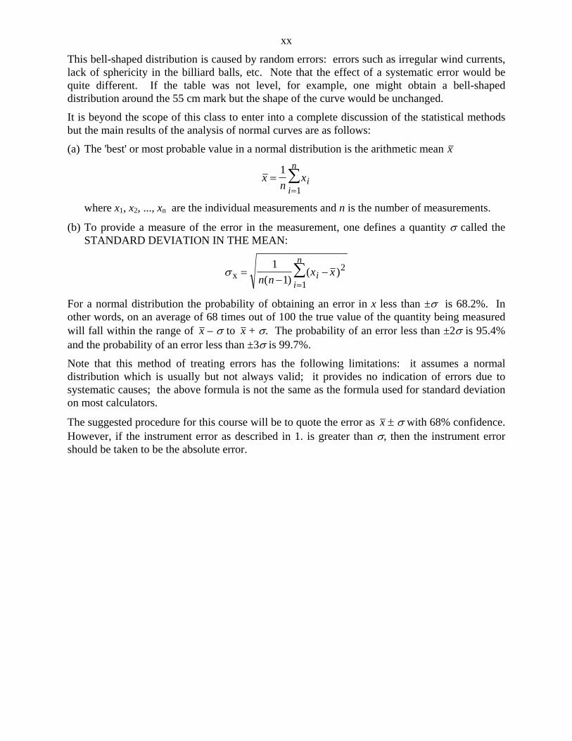
xx

This bell-shaped distribution is caused by random errors: errors such as irregular wind currents, lack of sphericity in the billiard balls, etc. Note that the effect of a systematic error would be quite different. If the table was not level, for example, one might obtain a bell-shaped distribution around the 55 cm mark but the shape of the curve would be unchanged.

It is beyond the scope of this class to enter into a complete discussion of the statistical methods but the main results of the analysis of normal curves are as follows:

(a) The 'best' or most probable value in a normal distribution is the arithmetic mean x

xn

xii

n

1

1

where x1, x2, ..., xn are the individual measurements and n is the number of measurements.

(b) To provide a measure of the error in the measurement, one defines a quantity called the STANDARD DEVIATION IN THE MEAN:

x

1

12

1n nx xi

i

n

( )( )

For a normal distribution the probability of obtaining an error in x less than ± is 68.2%. In other words, on an average of 68 times out of 100 the true value of the quantity being measured will fall within the range of x – to x + . The probability of an error less than ±2 is 95.4% and the probability of an error less than ±3 is 99.7%.

Note that this method of treating errors has the following limitations: it assumes a normal distribution which is usually but not always valid; it provides no indication of errors due to systematic causes; the above formula is not the same as the formula used for standard deviation on most calculators.

The suggested procedure for this course will be to quote the error as x with 68% confidence. However, if the instrument error as described in 1. is greater than , then the instrument error should be taken to be the absolute error.

xxi

G: PROPAGATION OF ERRORS IN CALCULATIONS In a number of cases the quantity of interest cannot be measured directly – it is calculated by using two or more directly measured quantities. When uncertain quantities are used in numerical calculations one usually wishes to know the error in the result. The simplest method, although not the most accurate, is to determine the maximum possible error. MAXIMUM POSSIBLE ERROR METHOD

CALCULUS TECHNIQUE

One technique for obtaining an error expression is to make use of calculus. If you are familiar with the rules for derivatives you will find this technique relatively simple.

Before proceeding, a brief review of some of the definitions and rules of differential calculus will be helpful.

Suppose y is some function of the variable x. Then the derivative of y with respect to x is dy/dx, sometimes denoted y'. Mathematicians speak of ‘d/dx’ as being the differentiation operator: ‘d( )/dx’ means ‘take the derivative with respect to x’ of whatever function is placed in the parentheses. ‘d( )/dx’ can also be considered to represent the small change d( ) that occurs in ( ), for a small change dx in x, divided by this small change in x.

Therefore, starting from

dy

dxy

and multiplying both sides by the small change dx in x, yields

dy = y dx

Therefore the small change in the variable y arising from a small change in the variable x is calculated by multiplying the small change in x by the derivative of y with respect to x.

The ‘small changes’ are called the DIFFERENTIALS of the appropriate variables.

The rules of calculus for calculating differentials are the same as those for calculating derivatives.

Suppose y = cxn,

Using the exponent rule, the DERIVATIVE of y with respect to x, dy/dx = y', is

dy

dxy ncx n 1

The DIFFERENTIAL of y is

dy = ncxn–1 dx

Similarly, if u, v, and w are functions of some (dummy) variable x:

d

dxu v w

du

dx

dv

dx

dw

dx( ) (derivative)

d(u + v – w) = du + dv – dw (differential)

xxii

d

dxuvw vw

du

dxuw

dv

dxuv

dw

dx( ) (derivative)

d(uvw) = vw du + uw dv + uv dw (differential)

d

dxu

vv du dx u dv dx

v

( / ) ( / )2

(derivative)

d uv

vdu udv

v

2

(differential)

d

dx

d

dx(sin ) cos

(derivative)

d(sin) = cos d (differential)

Application of these rules of calculus to calculation of errors proceeds as follows:

1. Ensure that the original expression is in its simplest form and that each variable is independent of all other variables. You may also find it easier if you replace division with multiplication and negative exponents. e.g. replace a/b with ab–1.

2. Calculate the differential of the expression. (Each symbol representing a measured value is taken as a variable to be differentiated.)

3. Take the absolute value of each term in the differential expression. A TERM is defined as an expression containing ONE differential quantity. e.g. (a/b) dx, uvw dx, y dv, (a–b) dx. The expression (dx – dy) is TWO terms:

(dx – dy) = dx – dy = dx + (–dy)

The effect of this rule is that (dx – dy) becomes

|dx| + |–dy| = dx + dy

i.e. The terms in the differential expression add.

4. Whenever the differential of any variable appears, substitute the absolute error of that variable.

5. When angles are used, the absolute error of the angle must be expressed in radians (not degrees).

The following examples illustrate this technique.

Example 1

The equation for kinetic energy is KE = 12 mv2 where m and v are mass and speed respectively.

The differential of KE is:

dKE = 12 dm v2 + 1

2 m 2v dv

Thus the absolute error of K is:

KE = 12 m v2 + 1

2 m 2v v

where m and v are the absolute errors in m and v.

xxiii

Example 2

The equation for centripetal acceleration is aR

v2

, where R and v are the trajectory radius and

speed of the object undergoing centripetal acceleration. Writing the equation as a = v2R–1, the differential of a is:

da = 2v dv R–1 + v2 (–R–2) dR

Applying rules 3 and 4 yields

a = 2v v R–1 + v2 R–2 R

where v and R are the absolute errors in v and R.

NON-CALCULUS TECHNIQUE

Addition and Subtraction

Consider the sum of two measurements, 25.4 ± 0.1 cm and 7.5 ± 0.2 cm. The result is 32.9 cm. To find the error in this result, consider that the first measurement lies between 25.3 and 25.5 cm. The second measurement lies between 7.3 and 7.7 cm. Therefore the sum lies between 32.6 and 33.2 cm, which may be written as 32.9 ± 0.3 cm. The absolute error in the result is the sum of the absolute errors of the two measurements. In symbolic form this may be written:

(a ± a) + (b ± b) = (a + b) ± (a + b)

To generalize:

if P = Q1 + Q2 + ... + Qn

where Q1, Q2, ... Qn are all measured quantities,

then P = Q1 + Q2 + ... + Qn

Now consider the subtraction of the two measurements from the previous discussion. The result is 25.4 cm – 7.5 cm = 17.9 cm. The limits of the range of the result are obtained by calculating

(25.4 cm + 0.1 cm) – (7.5 cm – 0.2 cm) = 25.5 cm – 7.3 cm = 18.2 cm

and

(25.4 cm – 0.1 cm) – (7.5 cm + 0.2 cm) = 25.3 cm – 7.7 cm = 17.6 cm

Thus the result is expressed as 17.9 ± 0.3 cm. Thus when quantities are subtracted the absolute error in the result is the sum of the absolute errors in the quantities.

Combining this with the result for addition, if P is calculated from the addition and/or subtraction of a number of measured quantities Qi,

P = Q1 + Q2 – Q3 – Q4 + ... + Qn

then P = Q1 + Q2 +Q3 + Q4 + ... + Qn

WHEN QUANTITIES ARE ADDED OR SUBTRACTED THE MAXIMUM POSSIBLE ABSOLUTE ERROR IN

THE RESULT IS THE SUM OF THE ABSOLUTE ERRORS IN THE QUANTITIES.

xxiv

Multiplication

Consider a rectangle measured to have sides a ± a and b ± b. The area A and its absolute error A are calculated as follows:

A±A = (a ± a)( b ± b) = ab ± (a)b ± ab) ± (a)b)

Factoring the product ab yields:

A A aba

a

b

b

a b

ab

1( )( )

Noting that ab = A, and ignoring the second order term (a)(b)/ab since it will be small compared to the other terms in the square brackets, yields:

A A

a

a

b

b

i.e. A

A

a

a

b

b

In general, if P is the product of measured quantities Q1, Q2, ... Qn, then the relative error in P is

P

P

Q

Q

Q

Q

Q

Qn

n 1

1

2

2

THE MAXIMUM POSSIBLE RELATIVE ERROR IN A PRODUCT IS THE SUM OF THE RELATIVE

ERRORS IN THE FACTORS. Noting that relative and percentage errors are related by % error = 100 × (relative error), the maximum possible percentage error in a product is the sum of the percentage errors in the factors. Division

Let P be the result of the division of Q by R.

i.e. PQ

R

Then

P PQ Q

R R

QQ

Q

RR

R

Q

R

Q

QR

R

1

1

1

1

Applying the binomial expansion and ignoring 2nd order terms yields:

P PQ

R

Q

Q

R

RP

Q

Q

R

R

1 1

so

P PQ

Q

R

R

i.e. P

P

Q

Q

R

R

xxv

THE MAXIMUM POSSIBLE RELATIVE ERROR IN A QUOTIENT IS THE SUM OF THE RELATIVE

ERRORS IN THE DIVISOR AND DIVIDEND. Powers and Roots

Using the result obtained for multiplication and realizing that the expression Qn means to multiply Q by itself n times, if

P = Qn then

P

Pn

Q

Q

THE MAXIMUM POSSIBLE RELATIVE ERROR IN RAISING A BASE VALUE TO AN EXPONENT IS THE

PRODUCT OF THE EXPONENT AND THE RELATIVE ERROR IN THE BASE.

For a more general example, consider the quantity N given by the following expression:

N = (AB4)/(CD½)

where A, B, C, D are all measured quantities. The maximum possible relative error in N is

N

N

A

A

B

B

C

C

D

D 4 ½

Note that the error in N is influenced more by errors made in measuring B than any of the other quantities. In designing and performing such an experiment great care should be taken to measure B with the highest degree of precision attainable. SUMMARY

1. All measured quantities have associated with them an uncertainty which can be expressed as an absolute or relative error and which limits the number of significant figures of these quantities and any results calculated from them.

2. When uncertain quantities are added or subtracted the maximum possible absolute error of the result is determined by adding the absolute errors of the separate quantities.

3. When uncertain quantities are multiplied or divided the maximum possible relative error of the result is determined by adding the relative errors of the separate quantities.

4. When an uncertain quantity is raised to a power (including a fractional power) the maximum possible relative error in the result is determined by multiplying the relative error in the quantity by the exponent.

5. When uncertain quantities are related in more complicated ways (e.g. log functions, trigonometric functions) the result must be calculated twice, once with the experimental values and then with the extreme values of the quantities. The maximum possible absolute error is the difference between these two values of the complicated function.

xxvi

ADDITION IN QUADRATURE METHOD

For the purposes of this laboratory, it is sufficient to use the maximum possible error as the error in the result of a calculation. The following discussion of the addition in quadrature method is included for completeness and because it is the method most often used by scientists.

Because of the assumed random nature of experimental errors the maximum possible error overestimates the error in the result of a calculation. It is unlikely that all the errors in the uncertain quantities will be in the same ‘direction’, which is what is assumed in the maximum possible error method. A more accurate estimate of the propagation of errors through calculations is obtained by adding the errors in quadrature: the ‘sum of the errors’ is replaced by the ‘square root of the sum of the squares of the errors’.

Thus the absolute error in the result of addition and/or subtraction of uncertain quantities is the square root of the sum of the squares of the absolute errors in the uncertain quantities. If

P = Q1 + Q2 + Q3 + … + Qn

then

P = ( )Qii

2

Similarly, the relative error in the result of multiplication and/or division of uncertain quantities is the square root of the sum of the squares of the relative errors in the uncertain quantities. If

P = QR/T

then

P

P

Q

Q

R

R

T

T

2 2 2

Powers and roots are handled in a similar manner. If

N = (AB4)/(CD1/2)

then

N

N

A

A

B

B

C

C

D

D

2 2 2 2

41

2

xxvii

ERROR CALCULATION QUESTIONS

These questions are designed to help you in reviewing error calculations. In each of the questions you will be given an equation and some data to use in the equation. Each question consists of four parts.

(a) Derive the error equation. The error equation should be in symbols only.

(b) Use the data to do the calculation. Watch your significant figures and the units.

(c) Calculate the absolute error.

(d) Express the answer, with its absolute error, to the appropriate number of significant figures.

SAMPLE

The equation for kinetic energy is KE = 12 mv2 where m and v are mass and speed

respectively. Suppose that the following values were obtained in an experiment:

m = 5.32 ± 0.03 kg and v = 2.37 ± 0.07 m/s

(a) KE = 12 m v2 + 1

2 m 2v v where m and v are the absolute errors in m and v.

(b) KE = 12 (5.32 kg)(2.37 m/s)2 = 14.94 kgm2/s2 = 14.9 J

(c) KE = 12 (0.03 kg)(2.37 m/s)2 + 1

2 (5.32 kg)(2)(2.37 m/s)(0.07 m/s) = 0.967 J

(d) KE = 14.9 ± 1.0 J 1. The equation of an ellipse is

y bx

a= 1

2

2 ,

a = 22.6 ± 0.1 cm, b = 46.9 ± 0.1 cm, x = 12.2 ± 0.1 cm: y = 39.48 0.29 cm

2. From Kepler's third law of planetary motion, the orbital period T of a satellite in a circular

orbit at height h above a massive body of radius R and mass M is:

TR h

GM= 2

3

( ),

R = (1.738 ± 0.001) × 106 m; h = (1.1 ± 0.1) × 106 m

G = 6.67 × 10–11 N·m2/kg2; M = (7.35 ± 0.01) × 1022 kg

T = (1.357 0.073) 104 s 3. Consider an Atwood's machine in which the pulley is neither frictionless nor massless. In

that case the acceleration is

am m g

I R m m m

( )

( / )2 1

21 2

where I is the moment of inertia of the pulley, R is its radius and m is a mass that is used to counteract the friction. Given g = 980 cm/s2, m1 = 100 ± 1 g, m2 = 200 ± 2 g,

I = 950 ± 50 g·cm2, R = 3.5 ± 0.1 cm and m = 5.0 ± 0.1 g: a = 256 15 cm/s2.

xxviii

4. When resistances R1, R2, and R3 are connected in parallel the total resistance, R, is given by

the equation

1 1 1 1

1 2 3R R R R

Given: R1 = 50 5 , R2 = 70 5 , R3 = 95 5 . R = 22.3 1.8

xxix

H: SAMPLE CALCULATIONS For each different equation used in the analysis of an experiment a sample calculation (and possibly a sample error calculation) are required. The following discussion explains what is required in a proper sample calculation.

1. Label the calculation 2. State the values, with their units and experimental errors, that will be used in the sample

calculation. 3. State the equation in symbols. 4. Show the substitution of the values (with their units but not their experimental errors) in the

equation. 5. Give the result of the calculation (don’t worry about significant figures at this stage). 6. State the error equation in symbols. 7. Show the substitution of values (with units) in the error equation. 8. Give the result of the error calculation. 9. State the result and its absolute error with the appropriate number of significant figures.

The following rule is to be used in rounding off the results of calculations: ROUND OFF THE ABSOLUTE ERROR IN THE RESULT TO TWO SIGNIFICANT FIGURES, THEN ROUND OFF THE RESULT TO THE SAME NUMBER OF DECIMAL PLACES AS THE ABSOLUTE ERROR. If scientific notation is being used, express both the result and its absolute error to the same power of ten before applying the second part of this rule.

As an example, suppose the magnitude of the momentum of some object whose mass and speed have been measured is to be calculated. The following is the correct sample calculation:

1. Sample Calculation of Momentum (label)

2. m = 0.675 ± 0.001 kg (statement of values) v = 0.123 ± 0.005 m/s

3. p = mv (equation in symbols) 4. p = (0.675 kg)(0.123 m/s) (substitution of values) 5. p = 0.083025 kg·m/s (calculation result)

6. p = m v + m v (error equation in symbols)

7. p = (0.001 kg)(0.123 m/s) + (0.675 kg)(0.005 m/s) (substitution of values)

8. p = 0.003498 kg·m/s = 0.0035 kg·m/s (error calculation result)

9. p = 0.0830 ± 0.0035 kg·m/s (round off) p = (8.30 ± 0.35) × 10–2 kg·m/s

xxx

I: COMPARING TWO QUANTITIES Experiments sometimes involve determining a physical quantity by two different methods to see if the results of the two methods agree. Sometimes one wishes to compare the experimental results with the predictions of a theory. In either case it is highly unlikely that there will be exact numerical agreement between the values to be compared. To compare the quantities, and decide if there is agreement, their experimental errors must be calculated. If the ranges of the two values overlap the values are said to agree within the limits of the error of that experiment. If the ranges do not overlap, then the values do not agree.

For example, if one determines the value of g to be 979 ± 3 cm/s2 and the known value is 981 cm/s2 then the two values agree because the range of the experimental value (976 cm/s2 to 982 cm/s2) includes the known value.

Bar Graph Comparison gexp = 979 3 cm/s2

975 976 977 978 979 980 981 982 983 cm/s2 | | | | | | | | | | |

Algebraic Comparison

The test for error range overlap can be expressed quantitatively as follows. Let x1 x1 and x2 x2 be two values that are to be tested for agreement within experimental error. If the magnitude of the difference between the values is less than the sum of their absolute errors then the values agree.

i.e. if | x1 – x2 | x1 + x2

then x1 and x2 are said to be equal within experimental error. When experimental errors have not been computed, the experimental value is compared with the standard known value by computing the percentage difference:

%100valueknown

valueknownvaluealexperimentdifference%

When a physical quantity does not have an accepted value, the following equation is used to calculate the percentage difference between values determined by two experimental methods:

%100valuesmaller

valuesmallervaluelargerdifference%

When the percentage change in a value is to be calculated, the following equation is used:

%100valueinitial

valueinitialvaluefinalchange%

range of gexp values

gacc

1

E30A: AC MEASUREMENTS OF CAPACITANCE AND INDUCTANCE E30B: PHASE MEASUREMENTS IN AC CIRCUITS

THEORY In ac circuits, the three basic circuit elements are the resistor, the capacitor, and the inductor.

RESISTOR: Voltage and current are in phase and related by Ohm’s Law:

VR = IR

The average power dissipation is

P I RV

RVI 2

2

CAPACITOR: Voltage lags current by ¼-cycle (90)

Voltage and current are related by the equation

VC = XCI

where XC = 1/C = 1

2fC is the capacitive reactance of the capacitance C at

frequency f.

The average power dissipation is 0.

INDUCTOR: Voltage leads current by 90

Voltage and current are related by the equation

VL = XLI

where XL = L = 2fL is the inductive reactance of the inductance L at frequency f.

The average power dissipation is 0.

A. AC MEASUREMENTS OF CAPACITANCE AND INDUCTANCE Consider the circuit with a capacitor and resistor in series fed by an ac audio generator.

By Ohm's Law for capacitors, the capacitor voltage VC is given by

VC = XCI = 1

2fCI (1)

This can be rewritten as

I = (2CVC) f ,

which is a linear relation between the current, I, and the frequency, f, provided that the capacitance, C, and the voltage across the capacitor, VC, are constant.

An experimental plot of I versus f with VC maintained constant will give a straight line whose slope can be measured.

2

The value of the capacitance is then

C = slope of graph

2VC

(2)

where VC is the value of the constant voltage maintained across the capacitor.

Consider the circuit with an inductor and resistor in series fed by an ac audio generator.

By Ohm's Law for inductors, the inductor voltage VL is given by

VL = XLI = 2 fLI (3)

This can be rewritten as

VL = (2LI) f

which is a linear relation between the inductor voltage, VL, and the frequency, f, provided that the inductance, L, and the current, I, are constant.

An experimental plot of VL versus f with I maintained constant will give a straight line whose slope can be measured.

The value of the inductance is then

L = slope of graph

2I (4)

where I is the value of the constant current maintained through the circuit.

PROCEDURE The equipment consists of two digital multimeters, an audio generator, two carbon resistors (one 330 and one 820 or 1000 ) and a circuit board containing a capacitor and an inductor.

Using one of the digital multimeters as an ohmmeter, measure the resistances of the two given resistors.

A1. Connect the capacitor and the 820 or 1000 resistor in series with the audio generator. Connect one multimeter across the capacitor to measure VC. (Note that the meter gives the rms (effective value) voltage.) Connect the other multimeter across the resistor to measure VR. This enables the current to be determined indirectly by using

Irms = V

RRrms (5)

3

Starting at 2000 Hz, measure the resistor voltage at 1000 Hz intervals to 8000 Hz, keeping VC constant at 2.5 Vrms by adjusting the amplitude of the audio generator output as necessary.

A2. In the circuit used in A1, replace the capacitor with the inductor. Keeping the current constant (by maintaining a resistor voltage of 0.5 Vrms by adjusting the audio generator output amplitude as necessary), measure the inductor voltage, VL, for frequencies from 1000 to 4000 Hz in 500 Hz increments.

ANALYSIS

THERE ARE NO ERROR CALCULATIONS REQUIRED IN PART A.

A1. Use equation (5) to calculate the current at each frequency. Plot the graph of current versus frequency, determine the slope, and use equation (2) to calculate the capacitance.

A2. Use equation (5) to calculate the (constant) current. Plot the graph of inductor voltage versus frequency, determine the slope, and use equation (4) to calculate the inductance.

B. PHASE MEASUREMENTS IN AC CIRCUITS There is a simple method of measuring phase with an oscilloscope in x-y mode of operation (i.e. with both vertical and horizontal input voltages, the sweep circuitry being disconnected). This method is very convenient for phase measurements because the gains of the vertical and horizontal oscilloscope amplifiers do not need to be the same. This is in contrast to the measurement of polarization ellipses (elliptical Lissajous figures) in which case incorrectly shaped ellipses will be obtained if the vertical and horizontal gains are not equal.

The experimental technique for phase-measuring is simple. Referring to the ellipse shown, the phase difference between the vertical input voltage Vy and the horizontal input voltage Vx is given by

y – x = sin–1 A

B

or sin( y – x) = vertical height at centre of ellipse

total vertical height of ellipse

In the case of an ellipse whose major axis is aligned with the x or y directions as shown, the values of A and B are the same, so

y – x = sin–1 (1) = / 2

x

y

x

y

4

which is a result known from Lissajous figures, i.e. a 90 phase difference between the orthogonal x and y oscillations leads to an ellipse whose axes are aligned with the x and y axes (or, as a special case, a circle).

The theoretical support for the measurement of phase angle is very simple.

Consider two ac voltages Vy, Vx of the same frequency . The voltage Vy, given by

Vy = Voy sin ( t + y)

is applied to the vertical input while the voltage

Vx = Vox sin ( t + x)

is applied to the horizontal input. Suppose that the gains of the vertical and horizontal amplifiers are not equal, and that they are given by Gy and Gx. Then the voltages appearing on the scope will be

Vy = GyVy = GyVoy sin ( t + y) (6)

and

Vx = GxVx = GxVox sin ( t + x) (7)

where the x-y coordinate system has its origin at the centre of the ellipse.

The central vertical half-height 12 A is obtained by

setting Vx = 0 in equation (7) above, which gives

t + x = 0 or t = – x

and then by substituting this result into (6), giving

Vy centre = 12 A = GyVoy sin ( y – x) (8)

Equation (8) can be re-arranged to give

sin ( y – x) = 12 A

G Vy oy

(9)

The next step is to realize that the height 12 B of the ellipse, i.e. the maximum y-value, is obtained

when, in equation (6),

sin ( t + y) = 1

at which time Vy = Vy max = 12 B = GyVoy (10)

Substituting (10) into (9),

sin ( y – x) = 12

12

A

B

A

B (11)

5

which is the desired result. Note that the unequal gains Gx and Gy do not affect this measurement, since (9) can be written as

sin ( y – x) = G V

G V

A

By oy y x

y oy

sin( )

12

12

which shows that the gain Gx doesn’t appear in the calculation, and the gain Gy cancels out.

CIRCUIT THEORY The phase ellipse method will be used to measure phase differences between voltages in series resistor-capacitor and series resistor-inductor circuits.

In the following circuit the audio generator is connected to the capacitor and resistor which are connected in series. The phase difference between the capacitor and resistor voltages can be calculated by considering the phasor diagram of these voltages, plotted with the reference axis taken to be in phase with the common current.

The phase T of the total voltage Vac with respect to the current is given by

tan T = V

V

X I

RI

X

R CRC

R

C C 1

while the phase R of the resistor voltage Vbc with respect to the current is 0 (voltage and current are in phase across a resistor). The phase difference between these two voltages is thus

= T – R = tan–1 1

CR

– 0 = tan–1

1

CR

(12)

Solving for the capacitance yields

C = 1

2 fR tan (13)

Consider the following circuit in which the audio generator is connected to the inductor and resistor which are connected in series.

6

As was done for the series R-C circuit, the phase difference between the inductor and resistor voltages can be calculated by considering the phasor diagram of these voltages, plotted with the reference axis taken to be in phase with the common current.

The phase T of the total voltage Vac with respect to the current is given by

tan T = V

V

X I

RI

X

R

L

RL

R

L L

while the phase R of the resistor voltage Vbc with respect to the current is 0 (voltage and current are in phase across a resistor). The phase difference between these two voltages is thus

= T – R = tan–1 L

R

– 0 = tan–1

L

R

(14)

Solving for the inductance yields

L = R

f

tan2

(15)

PROCEDURE The equipment consists of an oscilloscope, the audio generator, a 330 resistor, and the circuit board containing the capacitor and inductor.

B1. Connect the capacitor and 330 resistor in series with the audio generator (see circuit diagram in Theory).

Set the audio generator frequency to 70 kHz (i.e. 70,000 Hz).

Apply the total circuit voltage Vac to Channel 2 of the oscilloscope by connecting leads from the audio generator sine wave output terminals to the CH 2 scope input terminals (be sure to match red and black terminals). Apply the resistor voltage Vbc to Channel 1 of the scope by connecting the CH 1 input terminals to either side of the resistor. Be sure that the black scope terminal is connected to the side of the resistor that is connected to the black audio generator terminal. Put the scope in X-Y mode by pushing-in the X-Y button on the upper right portion of the scope, setting the TRIG SOURCE switch to the upper X-Y position, and setting the VERT MODE switch to the X-Y position.

Using the phase ellipse method (see Theory and Experiment E31) measure the vertical height at centre of ellipse, A, and total vertical height of ellipse, B, for the phase ellipse caused by the phase difference between Vac and Vbc. Remember to also determine the sign of the phase difference. To determine the sign of the phase difference push the X-Y switch so that it is in the

7

out position and set the VERT MODE switch to DUAL so that the actual sine waves Vac (Channel 2) and Vbc (Channel 1) are displayed. If Vac leads Vbc then the phase difference is positive and if Vac lags Vbc then the phase difference is negative.

B2. In the circuit used in part B1, replace the capacitor with the inductor.

Set the audio generator frequency to 300 Hz.

Measure the appropriate phase ellipse dimensions for the phase difference between the total voltage Vac and the resistor voltage Vbc. Determine the sign of the phase difference.

ANALYSIS The sine of the phase difference between the two signals input to the oscilloscope is determined by measuring the vertical height at the centre of the ellipse, A, and the total vertical height of the ellipse, B, and using

sin = A/B (16)

Error calculations are required in this part of the experiment. To help with these calculations, note the following relations:

cos = A

B

A B

B

2 (17)

so =

AB

A BB

2

cos (18)

which is the error in the phase difference calculated using equation (16). Note that this error value is in radians (which is what you want, see 5. on page xxii).

Also, (tan ) = sec2 (19)

Substitution of equation (18) into (19) is then used with equations (13) and (15) to calculate the experimental errors in C and L respectively.

B1. Use equation (16) to calculate the phase difference, , between the total voltage and resistor voltage.

Use equation (13) to calculate the value of the capacitance and its experimental error. How does this value compare with that obtained in part A1?

B2. Use equation (16) to calculate the phase difference, , between the total voltage and resistor voltage.

Use equation (15) to calculate the value of the inductance and its experimental error. How does this value compare with that obtained in part A2?

8

E31: PHASOR ANALYSIS

OBJECT An ac source is connected to simple series and parallel circuits and phasor analysis is used to determine the impedances of the unknown components.

THEORY A phasor is a rotating vector which represents the time variation of a sinusoidal quantity. A phasor diagram is a two-dimensional phasor plot which shows the magnitude and phase angle for the associated sinusoidal wave at a particular time. Phasor diagrams are useful for showing phase differences between two or more sinusoidal quantities.

As an example of the phasor diagram of a sinusoidal voltage, consider the following:

e = 100 sin ( t + 60°) volts

This voltage would be shown on a phasor diagram as:

(The phasor magnitude is usually taken to be the effective (rms) value of the associated wave.)

As with vectors, phasors can be represented in two ways, polar or rectangular. Polar notation specifies the magnitude (effective value) and phase angle of the phasor quantity while rectangular notation specifies the horizontal (real) and vertical (imaginary or j) components of the phasor.

The phasor shown in the following diagram can be represented by both notations as follows:

Polar: eff. value phase angle

A = A

Rectangular: horizontal + j vertical

A = b + jc

Conversion between the two forms of notation is done by using trigonometry to obtain the following relations:

horizontal component = b = A cos vertical component = c = A sin

magnitude = A = b c2 2 phase angle = = arctan (c/b)

Phasor addition or subtraction is done in the same way as for vectors. Rectangular representation is used and the corresponding horizontal and vertical components are added or subtracted.

e.g. if A = 8 + j4 and B = 3 – j2, then A + B = (8 + 3) + j(4 + –2) = 11 + j2

9

Unlike vectors, phasors can also be multiplied or divided. This is done as follows. Polar representation is used. For multiplication, the magnitudes are multiplied and the phase angles are added. For division, the magnitudes are divided and the phase angles are subtracted.

e.g. if A = 4530° and B = 1520°, then A/B = (45/15) (30° – 20°) = 310°

In this lab, phase angles are measured by use of the phase ellipse method (see the Theory for E30 for a derivation of the phase ellipse method equation). The phase ellipse is formed by switching off the internal sweep circuitry of the oscilloscope (X-Y mode). This is done by pushing-in the X-Y button on the upper right portion of the scope, setting the TRIG SOURCE switch to the upper X-Y position, and setting the VERT MODE switch to the X-Y position. If the sinusoidal voltages applied to Channel 1 and Channel 2 of the oscilloscope are out of phase, the oscilloscope display will be an ellipse (if the voltages are in phase, the display will be a straight line with a non-zero slope). The magnitude of the phase angle between the CH 1 and CH 2 signals is then calculated from the arcsine of the ratio of the vertical height at the centre of the ellipse (A) to the total vertical height of the ellipse (B).

A = vertical height at centre of ellipse

B = total vertical height of ellipse

= phase angle between the applied voltages

= arcsin A/B

sin = A/B

To determine the sign of the phase angle, the oscilloscope is used in the normal swept mode and both sinusoidal signals are displayed. Remembering that the oscilloscope beam is swept from left to right across the screen, the signal that peaks ‘first from the left’ is leading in time. Thus in the following diagram signal 1 is ahead in time and has a positive phase angle with respect to signal 2.

A. SERIES CIRCUIT The series circuit shown in Figure A consists of three unknown impedances Z1, Z2, and Z3 and the known resistance RI = 1 k.

The resistor RI is used to determine the current in the circuit by an indirect method.

10

The emf supplied by the source, E, is the phasor sum of the voltage drops across the circuit components:

E = VI + V1 + V2 + V3 (1)

The current I supplied by the source is

I = V

RI

I

(2)

From Ohm’s Law, the total equivalent impedance of the circuit is

Zser = E

I (3)

To determine the values of the unknown impedances their individual voltage drops V1, V2, and V3 must be determined. However, because the audio generator and the oscilloscope used to measure voltages in this lab are connected through a common ground, these voltages cannot be measured directly. Instead the voltages VI, VA, VB, and E as shown in Figure A are measured and the following equations are used:

11

V1 = VA – VI (4)

V2 = VB – VA (5)

V3 = E – VB (6)

The individual impedances are then determined by

Zi = Vi / I (7)

and the total equivalent impedance of the series circuit is given by the phasor sum

Zser = RI + Z1 + Z2 + Z3 (8)

PROCEDURE NOTE: Although error calculations are not required for this experiment, be sure to record the experimental error in all measurements.

Set the frequency of the audio generator to 4 kHz (4,000 Hz).

Connect the unknown impedances and the resistor in series with the audio generator as shown in Figure A. (Note that the red terminal of the audio generator is connected to impedance 3 first.)

Set the multimeter for ac voltage. Connect the multimeter COM terminal and the oscilloscope CH 2 black terminal to the black terminal of the audio generator sine wave output.

Connect together a red lead from the multimeter V- terminal and a red lead from the oscilloscope CH 2 red terminal. This will be your ‘probe’ for measuring magnitude and phase of voltages.

Connect the red and black CH 1 scope terminals across RI. Be sure that the black terminal is connected to the side of the resistor that goes to the black terminal of the audio generator. The CH 1 voltage will be in phase with the current in the circuit and will be used as the reference for phase angle measurements.

To set the voltage input to the circuit, connect the voltage probe (the red leads from the multimeter and CH 2 of the scope) to the red terminal of the audio generator. Adjust the sine wave amplitude controls until the multimeter reads 6.0 V (rms). This is the magnitude of the voltage E.

Using the phase ellipse method (push-in the X-Y button on the upper right portion of the scope, set the TRIG SOURCE switch to the upper X-Y position, and set the VERT MODE switch to the X-Y position) measure the ellipse dimensions so that the phase angle of E with respect to the current in the circuit can be determined. Now push the X-Y switch so that it is in the out position, set the VERT MODE switch to DUAL to observe the two sine wave voltages (E and VI), and note the sign of the phase angle of E (+ or – with respect to the current).

Now connect the voltage probe to the appropriate points in the circuit and measure the magnitudes, ellipse dimensions, and signs of the phase angles of the voltages VI, VA, and VB. (See Figure A.)

12

Record your data in a table similar to the following:

Voltage Phase Ellipse Measurements Sign of Phase ( __ V) Centre Height

( __ cm) Total Height

( __ cm) Phase Angle (+ / –)

Angle (°)

E

VI

VA

VB

ANALYSIS REMEMBER THAT ALL EQUATIONS IN THE THEORY ARE PHASOR EQUATIONS.

No error calculations are required for this experiment.

Throughout the analysis state all phasor results in both polar and rectangular notation.

Using equation (2) calculate the current, I.

Using equations (4), (5), and (6) calculate the voltages V1, V2, and V3.

On a carefully labelled scale phasor diagram, plot the graphical addition of VI, V1, V2, and V3 by drawing the phasors tip to tail. Choose the reference (horizontal) axis to be in phase with the current. (Thus VI will lie along the reference axis.) On the graph, measure the magnitude and phase angle of the graphical phasor sum VI + V1 + V2 + V3.

Compare the magnitude and phase angle of this resultant voltage with the directly measured magnitude and phase angle of E by calculating the percentage difference between the graphical and calculated magnitude of E and calculating the percentage difference between the graphical and calculated phase angle of E.

Use equation (7) to calculate the individual unknown impedances, Z1, Z2, and Z3. For each of the unknown impedances identify the type of impedance (resistive, capacitive, inductive, resistive-capacitive, or resistive-inductive).

Use equation (8) to calculate the phasor sum of the individual impedances, i.e. calculate the total equivalent series impedance of the circuit. Now calculate the equivalent impedance as given by Ohm’s Law (equation (3)). Compare these two values for the equivalent impedance by calculating their percentage difference.

13

B. PARALLEL CIRCUIT

The circuit shown in Figure B1 consists of the two parallel unknown impedances Z2 and Z3 in series with the resistor RI. Z1 is not used in this part of the lab. The total unknown impedance of the parallel section, ZT, is related to Z2 and Z3 through

1 1 1

Z Z ZT 2 3

(9)

The admittance Y is defined as

Y = G + jB = 1/Z (10)

where G is the conductance and B is the susceptance. Y, B, and G are measured in Siemens (S = –1). The total admittance of the parallel part of the circuit is the sum of the two unknown admittances

YT = Y2 + Y3 (11)

The circuit shown in Figure B2 is used to determine the current flowing in each branch (in this figure in the right one) of the parallel arrangement. It is desired to know the current I30 (or I20) in the absence of the resistor RI (i.e. the current that would flow if the resistor had zero resistance). Assuming E is kept constant at 6.0 V and the resistance of RI is set to 0,

E = I30 Z3 (12)

and

14

E – VI3 = I3 Z3. (13)

Since I3 = VI3 / RI , (14)

solving (12) for Z3 and substituting this result and (14) into (13) yields

I30 = EV

E V RI3

I3 I( ) (15)

I20 can be determined in a similar manner.

PROCEDURE The rms output voltage of the audio generator is to be kept constant at 6.0 V (as measured with the digital multimeter) at all times. Since the internal impedance of the generator is not negligible compared with the load impedance, whenever the circuit (load) is changed, the source voltage must be readjusted to 6.0 V. As for part A, the frequency of the generator is set to 4 kHz.

Connect the circuit as shown in Figure B1.

Set the multimeter for ac voltage. Connect the multimeter COM terminal and the oscilloscope CH 2 black terminal to the black terminal of the audio generator sine wave output.

Connect together a red lead from the multimeter V- terminal and a red lead from the oscilloscope CH 2 red terminal. This will be your ‘probe’ for measuring magnitude and phase of voltages.

Connect the red and black CH 1 scope terminals across the sine wave output terminals of the audio generator. The CH 1 voltage will be in phase with the voltage applied to the circuit, E, and will be used as the reference for phase angle measurements. Connect the ‘voltage probe’ to the red terminal of the audio generator sine wave output and adjust the sine wave amplitude controls until the multimeter reads 6.0 V (rms). This is the magnitude of the voltage E.

Connect the ‘voltage probe’ to the appropriate point in the circuit and measure the magnitude and phase angle with respect to E (including sign) of the resistor voltage, VI.

Connect the circuit as shown in Figure B2.

Connect the voltage probe to the red terminal of the audio generator output and readjust the sine wave amplitude controls until the multimeter again reads 6.0 V.

Connect the voltage probe to measure the magnitude and phase angle (with respect to E) of the resistor voltage VI3.

Now reconnect the circuit with the resistor placed in the left branch. Connect the voltage probe to the red terminal of the audio generator and readjust the audio generator output to 6.0 V.

Connect the voltage probe to measure the magnitude and phase angle (with respect to E) of the resistor voltage VI2.

15

ANALYSIS Remember that all equations in the theory are PHASOR equations.

Using the measured values of VI and E in equation (4) calculate the equivalent impedance of the parallel combination. Calculate the equivalent admittance using equation (10).

Calculate I30 and I20 using the measured values of VI3 and VI2 in equation (15).

Calculate I0 (the total current in the circuit if the resistance of RI goes to 0) from I0 = E YT.

On a carefully labelled phasor diagram plot the graphical addition of I30 and I20. Choose the reference (horizontal) axis to be in phase with the applied voltage E. Measure the magnitude and phase angle of the graphical phasor sum of I30 and I20. Compare the magnitude and phase angle of this resultant current with the calculated magnitude and phase angle of I0.

Calculate the admittances of the individual unknown components using Y2 = I20/E and Y3 = I30/E. Using equation (10), calculate the impedances of the unknown components. Compare these values for Z2 and Z3 with the ones determined in Part A of this experiment.

16

36: ELECTRIC CURRENT BALANCE

OBJECT The object of this experiment is to use a technique by which an absolute determination of the Ampere can be made in terms of the forces between parallel current-carrying wires.

THEORY

Figure 1 The current balance is illustrated in Figure 1. It consists of a movable coil and a pair of stationary coils. The three coils consist of ten turns of #20 enamelled, single-cotton-covered magnet wire. The movable coil is pivoted on two knife edges so that it can rotate about a horizontal axis AA through these knife edges.

Consider the wires at the left end of the apparatus as shown in Figure 1. The current Is in the top wire of the stationary coil is parallel to the current Im in the movable coil. Thus, the movable coil experiences an upward magnetic force of attraction toward the top of the stationary coil, causing a torque about the horizontal axis AA. Furthermore, the movable coil current Im is anti-parallel to the current Is in the bottom part of the stationary coil, so there is a magnetic force of repulsion between these currents. This repulsion force is again upward on the movable coil thereby doubling the torque about the horizontal axis.

Examining the horizontal currents on the right side of the current balance shows that the right side of the movable coil experiences two downward magnetic forces, a repulsion from the antiparallel current in the top of the stationary coil and an attraction toward the parallel current in the bottom part of the stationary coil. The result is again a torque on the movable coil.

The net result of the upward forces on the left end of the movable coil and the downward forces on the right end is a magnetic torque which causes the plane of the movable coil to rotate clockwise about the horizontal axis AA as seen from a front view of Figure 1.

Attached to the movable coil are two rods carrying two sliding weights – one large and one small. The sliding weights can be moved to provide gravitational torques which counteract the

17

magnetic torque, and hence can be used to bring the movable coil to equilibrium, as explained in the following discussion.

Consider the cross-sectional view of the current balance shown in Figure 2. On the left, the currents in the top stationary coil and the movable coil are parallel, so there is an upward magnetic force of attraction on the movable coil with magnitude given by

FB = BsnmIm

where Bs =

0 s s

22

n Is is the magnetic field, at the position of the movable coil, due to the current

Is in the top part of the stationary coil, s/2 is the separation between the stationary and movable coils at equilibrium, Im is the current in the movable coil, ns and nm are the number of turns in the stationary and movable coils respectively, and is the length of the left end of the movable coil that is parallel to the wires in the stationary coil.

Substituting for Bs yields

FB =

0 s s m m

22

n I n Is

(1)

Also on the left side there is an upward force FB (identical to that of equation (1)) which arises due to the repulsion between the antiparallel currents in the movable coil and the bottom part of the stationary coil. The total clockwise torque on the movable coil due to the forces on the left side of the movable coil is thus:

= 2FBd (2)

where d is the distance between the supporting knife edge and the outer edge of the movable coil.

Because of the current directions, the right side of the movable coil experiences a net downward force of 2FB, and the torque due to this force is also clockwise with a magnitude of 2FBd. The total clockwise magnetic torque is thus

mag = 4FBd

18

mag = 4

0

22

2 2

n Is

d (3)

where I = Is = Im and n = ns = nm because the coils are series-wired and all have the same number of turns (10).

The clockwise magnetic torque is now counterbalanced by means of a gravitational torque provided by the sliding aluminum weights.

The current-direction switch on the apparatus is set so that when the current I is sent through the current balance, the end of the movable coil near the reference scale goes upward. This magnetic torque is now counterbalanced by a gravitational torque, SW, produced by the sliding large and small aluminum weights.

SW = mLgrL + mSgrS (4)

where r refers to the distances the masses have been moved from their initial positions and the subscripts L and S refer to ‘large’ and ‘small’ respectively.

At equilibrium,

SW = mag (5)

Substitution from equations (4) and (3) yields

mLgrL + mSgrS = 4

0

22

2 2

n Is

d (6)

Solving for I yields

I =

g s

n dm r m r

4 2o

L L S S (7)

or I = k m r m rL L S S (8)

where k =

g s

n d4 2o

(9)

is a constant for each particular apparatus that depends on the fixed dimensions s,, and d and the number of coil turns, n. Equation (8) shows that current can be determined in terms of gravitational torques. This technique, with more refined equipment, is used by Standards Laboratories to define the ampere.

EXPERIMENT 1. Measure s, the average height of the stationary coils, , the average width of the movable

coil, and d, the average distance from the knife edge axis to the ends of the movable coil. Record mL and mS, the masses of the large and small aluminum weights.

2. Adjust the large and small aluminum weights so that they are at the 1 cm mark (closest to the central axis of the movable coil.

19

3. Balance the movable coil, by adjusting the positions of the threaded weights on the brass rods until the pointer on the movable scale aligns with the reference mark on the apparatus. (See note below the table on the next page.)

4. Connect the circuit shown in the following diagram:

The 5 rheostat across the power supply is used as a voltage divider to supply a variable current to the current balance.

5. Pass a current of 1.0 A through the current balance and adjust the reversing switch so that the pointer on the end of the movable coil moves upward relative to the reference mark. Counterbalance the resulting magnetic torque by moving the sliding aluminum weights until the movable coil returns to equilibrium (as indicated by the pointer aligning with the reference mark). Record the final positions of the large and small aluminum weights. Refer to the sample table for a suggested method of recording your measurements and results.

6. Repeat step 5. for currents of 2.0, 3.0, and 4.0 A.

ANALYSIS g = 9.81 m/s2 o = 4 10–7 Tm/A n = 10

1. Use equation (9) to calculate the value of k for your apparatus.

2. Use equation (8) to calculate the theoretical current for each data set. Note that rL and rS are the net displacements of the large and small weights from their initial positions,

i.e. r = final position – initial position

Compare the theoretical currents obtained from your current balance measurements with the currents measured directly with the ammeter.

Do your results confirm the validity of the current balance method of determining current in terms of the forces between current-carrying wires?

20

DATA AND RESULTS FOR ELECTRIC CURRENT BALANCE:

s = __ __ cm = __ __ cm d = __ __ cm

n = 10 mL = __ __ g mS = __ __ g

Large Weight Initial Position: __ __ cm

Small Weight Initial Position: __ __ cm

Ammeter Large Weight Small Weight Calculated Current ( __ A)

Final Pos’n ( 0.1 cm)

rL ( __ cm)

Final Pos’n ( 1.0 cm)

rS ( __ cm)

Current (A)

1.00

2.00

3.00

4.00

NOTES ON POSITIONING THE WEIGHTS AND ESTIMATING THE ERROR IN THE WEIGHT POSITIONS:

1. Take the error in the initial positions of the weights to be 0.1 cm.

2. When balancing, move the weights by division increments. i.e. Ensure that the weights are aligned with one of the distance marks on the rods.

3. Take the error in the final position of the large weight to be 0.1 cm.

4. Take the error in the final position of the small weight to be 1.0 cm.

21

E50: ELECTROMAGNETIC INDUCTION: FARADAY’S AND LENZ’S LAWS

OBJECT The effects of Faraday’s Law and Lenz’s Law will be observed in this experiment. It is important that all results be interpreted in terms of the predictions of these laws.

INTRODUCTION Faraday’s Law: If a circuit is placed in a region of varying magnetic flux, an emf equal to the

time rate of change of the magnetic flux through the circuit is induced in the circuit

emf = – d

dt

In this experiment, the varying magnetic flux is produced by a varying magnetic field, so

emf – dB

dt

Lenz’s Law: For any closed circuit in a region of varying magnetic flux, the direction of the induced current which results from the induced emf is such that it produces a magnetic field that opposes the change in the magnetic flux.

EXPERIMENT A. PERMANENT MAGNET Connect the 300 turn coil to the galvanometer as shown below. Be sure that the coil B terminal is connected to the galvanometer red terminal. Set the rheostat to full resistance.

Take the bar magnet and rapidly push the North end into the square opening in the coil. Observe and record the polarity (+ or –) of the galvanometer deflection. Observe and record the polarity of the deflection as the bar magnet is rapidly withdrawn. Also observe and record whether there is a dependence of the magnitude of the deflection on the speed with which the magnet is moved.

Reverse the bar magnet (i.e. insert South pole first) and repeat the above observations of deflection polarity.

Repeat all the above observations with the 600 turn coil. Also observe and record whether there is a dependence of the magnitude of the deflection on the number of turns in the coil (for this you will have to try to move the magnet at the same speed as you did with the 300 turn coil).

22

Record your observations in a manner similar to the following:

Polarity of Galvanometer Deflection

Coil North in North out South in South out

300 turn

600 turn

Dependence on speed of magnet motion:

Dependence on # of coil turns:

To aid in analyzing the response of the galvanometer, note that the polarity of the galvanometer deflection indicates the polarity of the terminal connected to the red galvanometer post. Also, remember that current flows from positive to negative and that the coil is the source of emf in the circuit (so current flows out of the positive coil terminal, through the circuit, and back into the negative coil terminal).

The coils are wound as shown below – when viewed from above the winding is counterclockwise from terminal A to terminal B.

When terminal B is positive, indicating that current is flowing out of B, the induced magnetic field has a North pole at the top of the coil. When terminal B is negative, indicating that current is flowing into B, the induced magnetic field has a South pole at the top of the coil.

Based on the previous paragraph, interpret your deflection polarity observations in terms of the predictions of Lenz’s Law. Is there agreement? Discuss.

What does Faraday’s Law predict for the dependencies of deflection magnitude on magnet speed and number of coil turns? Do your observations agree with these predictions?

23

B. GENERATION OF ALTERNATING VOLTAGES Connect two 1200 turn coils in series, as shown below, so that the emf’s generated in the windings add constructively. Suspend the bar magnet in a holder above the coils.

Suspend the magnet directly over and about 1 cm above the coils. Wind the string and release the magnet so that it spins in a horizontal plane above the coils. Observe and record the response of the galvanometer and oscilloscope. Note any dependence of magnitude of response on speed of magnet rotation.

Adjust the magnet so that it is much higher above the coils. Again spin the magnet and note whether there is any dependence of instrument response on magnet-coil separation.

Place the two coils on the C core from the mounting frame and repeat the observations of galvanometer and oscilloscope response when the magnet is spun above the coils.

Compare all of your observations with the predictions of Faraday’s Law of Induction.

C. LENZ’S LAW Use a paper wedge to hold the I core in the 600 turn coil as shown. Place the coil on its side and suspend the aluminum ring so that the I core passes through the ring. Connect the circuit as shown.

24

Rapidly slide one of the rheostats from the maximum resistance position to the minimum resistance position and observe and record the motion of the ring. Bring the ring to rest and observe and record its motion as the rheostat is rapidly changed from the minimum resistance position to the maximum resistance position.

Explain the ring’s motion (toward or away from the coil) in terms of Lenz’s Law.

D. THE TRANSFORMER AND MAGNETIC CIRCUITS Procedure

Mount the 300 turn primary and 600 turn secondary coils on the C core in the mounting frame and complete the magnetic circuit with the I core. Be sure that the I core is clamped down firmly with the mounting frame and that its laminations align with those of the C core. Connect the circuit as shown. The variable ac supply (set for 10 V AC), 4.5 rheostat, AC ammeter, and 300 turn coil form the primary circuit and the 600 turn coil, AC ammeter, and 85 rheostat form the secondary circuit.

Connect the oscilloscope as shown so the primary voltage goes to channel 1 and the 600 turn coil voltage goes to channel 2.

1. Plug in the ac power supply. Set the 85 ohm rheostat to full resistance and the 4.5 rheostat for minimum primary voltage. Slowly adjust the primary voltage, VP, by adjusting the 4.5 rheostat, until the secondary current, IS, is 0.10 A (100 mA).

2. Record the secondary voltage VS (peak-to-peak Channel 2 voltage), primary current IP, and primary voltage VP (peak-to-peak Channel 1 voltage) for secondary currents from 0.10 to 0.26 A in increments of 0.04 A.

Note that IS is changed by reducing the 85 rheostat resistance. Do Not adjust the 4.5 rheostat once it has been set as described in step 1.

3. Disconnect a wire in the secondary circuit (i.e. disconnect one of the leads at the 85 rheostat), leaving the secondary open-circuit (IS = 0, RS = ). Record the primary and secondary voltages, VP and VS.

25

Use a table similar to the following:

IS Secondary Voltage (V) IP Primary Voltage (V) VS/ VP VS IS VP IP % Power ( _A) Displ.

( _cm) V/cm VS ( _A) Displ.

( _cm) V/cm VP (W) (W) Loss

0.10

0.14

0.18

0.22

0.26

0.00

Now the effect of introducing nonmagnetic ‘air’ gaps in the magnetic circuit will be examined under the condition of constant secondary current.

Set the 85 rheostat to full resistance and the 4.5 rheostat to zero primary voltage.

4. Loosen the mounting frame clamps and place a paper towel folded into 8 paper thicknesses between the C core and I core. Clamp the I core down firmly and increase the primary voltage by adjusting the 4.5 rheostat until the secondary current, IS, is 0.10 A.

Record VS, IP, and VP.

5. Repeat step 4. for 16 and 32 paper towel thicknesses.

BE SURE TO REDUCE THE PRIMARY VOLTAGE TO 0 BEFORE CHANGING PAPER THICKNESSES.

Use a table similar to the following:

IS = 0.10 A __ A

Paper Secondary Voltage (V) IP Primary Voltage (V) VS IS VP IP % Power Thickness Displ.

( _cm) V/cm VS ( _A) Displ.

( _cm) V/cm VP (W) (W) Loss

0

8

16

32

26

Theory If the transformer were ideal, i.e. no leakage losses or core heating, no eddy losses in the magnetic core, and no Joule heating in the windings, then the power VPIP delivered to the primary would equal the power VSIS transferred to the secondary.

VPIP = VSIS (1)

But the flux in such a case is completely contained in the magnetic circuit so the flux through the secondary and the flux through the primary are equal. Therefore, since the induced emf is

VS = NS d

dt

in the secondary

and

VP = NP d

dt

in the primary,

V

V

N

NaP

S

P

S

(2)

where a is called the turns ratio. From (1) and (2),

V

V

I

I

N

NaP

S

S

P

P

S

Analysis Calculate and tabulate values of primary power, VPIP, and secondary power, VSIS, for the measurements made in part 2. Does the power relation (1) hold for your results? i.e. Does VPIP = VSIS within experimental error?

Calculate the percentage power loss

% Power Loss = V I V I

V I

V I

V IP P S S

P P

S S

P P

100% 1 100%

Plot a graph of % Power Loss versus secondary current for the values measured in part 2. Where do the losses occur?

Calculate, tabulate, and plot the voltage ratio VS/VP versus secondary current for the values measured in parts 2. and 3.

Calculate and tabulate the primary power, VPIP, secondary power, VSIS, and % Power Loss for the values measured in parts 4. and 5. Plot a graph of % Power Loss versus paper thickness (‘air’ gap thickness). Include the zero air gap data previously obtained at IS = 0.10 A in part 2.

In the Conclusion discuss the significance of the shapes of the graphs.

27

E52: MAGNETIC CIRCUITS

OBJECT The ability of magnetic material to provide a path for magnetic flux, the magnetization and hysteresis curves for a magnetic material, and the effect of an air gap in a magnetic circuit are examined in this experiment.

THEORY A magnetic field is that region in which a magnetic material is acted upon by a magnetic force. It is convenient to visualize a magnetic field as consisting of invisible magnetic lines of force. A magnetic line of force represents the path along which a theoretical isolated magnetic pole would move from one pole of a magnet to the other. The term magnetic flux refers to the total number of lines of force in a magnetic field. Magnetic flux is given the symbol , and has SI units of Webers (1 Wb = 1 Vs). Magnetic flux in a magnetic circuit is the counterpart of electric current in an electric circuit. The number of flux lines passing perpendicularly through an area A, divided by the area, is the magnetic flux density, B.

B = /A (1)

and has units of Wb/m2 = Tesla (T).

Just as an electric current cannot flow in an electric circuit until a voltage source is connected, magnetic flux (magnetic lines of force) cannot be established until a magnetomotive force (mmf) is produced. In the case of an electromagnet such as a current-carrying solenoid, magnetic flux appears only when electric current flows in the solenoid. Therefore, magnetomotive force must be a direct result of electric current. The magnetomotive force () produced by a solenoid coil of N turns carrying a current I is NI. The unit of mmf is the ampere-turn. In general a solenoid coil is wound on a magnetic core that controls the path of the magnetic field. The path has a mean length measured along its centre line. Analogous to electric field intensity, the magnetic field intensity or magnetizing force, H, is defined as the mmf per unit length along the path of magnetic flux.

H =

NI (2)

and has units of ampere-turn/meter (A-t/m).

For a particular magnetizing force H, a core will develop a particular flux and a flux density B. Flux density in a magnetic material plotted against magnetizing force forms a magnetization or B-H curve. The opposition to the establishment of magnetic flux is called reluctance. It is defined as the ratio of the drop in mmf to the flux produced (compare with Ohm's law for resistance). The symbol for reluctance is , so

=

(3)

While reluctance relates to a given magnetic circuit, permeability indicates the ability of a type of material to permit the setting up of magnetic lines of force. The reluctance of a section of material of length and cross sectional area A and absolute permeability is given by

28

=

A (4)

Combining the previous two equations and the definitions of B and H yields

= B

H (5)

Since the permeability of free space (0 = 4 10–7 Wb/Am) is constant, the absolute permeability of another material can be expressed relative to the permeability of free space by

= r 0 (6)

where r is the dimensionless quantity called relative permeability. Note that for magnetic materials and r are not constant, but rather depend on B and H.

In part 1 of this experiment, the effect of varying the amount of magnetic material in the circuit is examined. For a constant (peak) mmf, the (peak) flux passing through the circuit will increase as the reluctance in the circuit decreases (equation (3)). The reluctance is reduced by increasing the number of welding rods (magnetic material) in the circuit. Since this essentially replaces a given volume of air (low permeability) with welding rod material (high permeability) the reluctance will decrease and the flux should increase.

In part 2 of the experiment, the magnetization and hysteresis curves will be plotted for a magnetic sample consisting of three welding rods.

In part 3, the effect of an air gap in a magnetic circuit is examined. Simple theory can be used to predict how the flux density should vary with an increase in the length of the air gap. In the following discussion the subscript ‘m’ refers to ‘in magnetic material’, ‘a’ refers to ‘in air’, ‘g’ refers to ‘with gap’, and ‘w’ refers to ‘without gap’.

Consider the following magnetic circuit:

The total mmf applied to the circuit must equal the drop in mmf across each element of the magnetic circuit.

NI = Ha g + Hm m (7)

Since H = B/

NI = B Bag g mg m

0

(8)

29

Although the magnetic flux around the magnetic circuit is constant, the flux density, B, is not, due to fringing in the air gap. Using Ag to denote the effective area of the air gap,

Bag = BmgA / Ag (9)

where A is the actual cross-sectional area of the magnetic material.

Substituting (9) into (8) yields

NI = Bmg{A

A

g

g0

+ m

} (10)

Noting that m = tot – g and taking r for the relative permeability of the magnetic material gives

NI = Bmg{A

A

g

g0

+ tot g

r

0

} (11)

By requiring that the applied mmf be kept constant, the ratio of the flux density in the magnetic material when there is an air gap to the flux density when there is no air gap can be calculated:

NI = Bw tot

r

0

when there is no air gap (12)

Therefore,

Bmg{A

A

g

g0

+ tot g

r

0

} = Bw tot

r

0

(13)

and

B

B A

A

mg

w

tot

r g

g

tot g

r

1 (14)

After simplification,

B

B A

A

mg

w g

tot

r

g

1

1 1

(15)

The effective cross-sectional area of the air gap can be calculated by making an empirical correction. The length of the gap is added to each cross-section dimension of the adjoining magnetic material, and this new area is calculated. Thus

Ag = (a + g)(b + g)

Ag = ab + gb + ga + g2

Ag = A + (a + b)g + g2 (16)

30

Making this substitution and again simplifying,

B

B A

A a b

mg

w g

tot

r

g g

1

1 12

( )

(17)

EQUIPMENT The source of magnetomotive force is a 600 t coil fed current from a PASCO 60 Hz ac supply. The 85 voltage divider rheostat allows the coil current to be varied and the 4.5 rheostat is included in the circuit so that the current may be determined with an oscilloscope.

The peak current can be determined by measuring the peak-to-peak rheostat voltage and dividing by twice the rheostat resistance. The peak applied magnetomotive force is thus

= NI = NV

RRp p

2 (18)

and if the length of the magnetic circuit is known, the magnetic field intensity is H = /.

Magnetic flux is detected by integrating the voltage induced in a 1200 t ‘search’ coil by using an RC integrator with R = 1.0 M and C = 0.33 F. The peak magnetic flux through the search coil is

= RC

N

V

d

C2

(19)

where Nd is the number of turns (1200) and VC is the peak-to-peak voltage across the capacitor.

31

EXPERIMENT 1. EFFECT OF MAGNETIC MATERIAL ON FLUX DENSITY Connect the following circuit:

The two coils should be positioned on their sides with their openings aligned and separated by about 2 cm.

Adjust the position of the slider of the 85 rheostat until the oscilloscope CH 1 voltage (the 4.5 rheostat voltage which is proportional to the mmf source current) is 2.0 V peak-to-peak.

Measure the peak-to-peak flux detector output voltage (CH 2, capacitor voltage which is proportional to magnetic flux and flux density).

Now place one welding rod (magnetic material) through the openings in the two coils. This will reduce the reluctance in the ‘magnetic circuit’ between the two coils. Adjust the 85 rheostat slider position until the mmf voltage (CH 1) is again 2.0 V and measure the flux detector output (CH 2).

Repeat the above measurement, keeping the mmf voltage (CH 1) constant by adjusting the 85 rheostat slider position, for 2, 3, 4, 6, 8, and 10 welding rods linking the coils.

ANALYSIS Plot the flux detector output (peak-to-peak capacitor voltage) vs. number of welding rods.

This plot shows the effect on the magnetic flux of reducing the reluctance in a magnetic circuit.

2. MAGNETIZATION AND HYSTERESIS CURVES (FOR WELDING ROD MATERIAL) The circuit to be used is the same as in 1. Place 3 welding rods through the coils.

Measure the peak-to-peak flux detector output voltage (CH 2) for peak-to-peak mmf voltages (CH 1) of 1 V, 2 V, 3 V, 4 V, 5 V, and maximum voltage. As before, the mmf voltage is varied by adjusting the 85 rheostat slider position.

32

With the 85 rheostat slider set for maximum mmf voltage, push-in the X-Y button on the upper right portion of the scope, set the TRIG SOURCE switch to the upper X-Y position, and set the VERT MODE switch to the X-Y position (this puts the scope in X-Y mode and the hysteresis curve should be displayed). If the hysteresis curve is tilted to the left rather than the right, reverse the CH 2 scope connections. Adjust the oscilloscope scales to obtain a good representation of the hysteresis curve and carefully draw the curve in your notebook.

ANALYSIS Plot flux detector output versus mmf voltage. Since the flux detector output voltage is

proportional to the flux density B and the mmf voltage is proportional to the current and hence magnetic field intensity H, this plot is ‘proportional’ to the B-H curve for the welding rod material.

Compare your sketch of the hysteresis curve with example curves in your textbook and comment.

3. EFFECT OF AN AIR GAP IN A MAGNETIC CIRCUIT You are given a laminated C-core and two pole pieces. Measure the cross-sectional

dimensions a & b and the mean length, tot, of the magnetic core material for no air gap.

The circuit to be used is the same as for the previous two parts of the experiment. Mount the 600 t and 1200 t coils on the C-core, place the black adjustable pole pieces on top with no gap between them, place this assembly in the mounting frame, and tighten the clamps.

Maintain peak magnetizing current constant by maintaining peak-to-peak mmf voltage (CH 1) at 0.8 V. Measure flux detector output voltages VC (CH 2) for air gaps of 0, 0.1 cm, and 0.2 to 1.0 cm in 0.2 cm increments.

Record your data and results in a table similar to the following:

Gap Flux Detector Output Flux Density gap/no gap Ratios

(cm) peak-to-peak displacement

(cm)

VOLT/DIV Voltage (V)

Experimental (Bmg/Bw)expt

Theoretical (Bmg/Bw)theo

0.0

0.1

0.2

0.4

0.6

0.8

1.0

Disconnect the 4.5 rheostat from the circuit and use the available multimeter to measure its actual resistance.

33

ANALYSIS Using the results for no air gap and equations (1), (2), (5), (6), (18), and (19) the following

equation for the relative permeability of the magnetic material can be derived:

r = (0.456 m/V) tot rh CR V

ab0

where tot is the mean length of the magnetic core material in metres, Rrh is the actual ‘4.5 ‘ rheostat resistance in ohms, VC0 is the peak-to-peak flux detector output voltage for 0 air gap in volts, and a & b are the magnetic core cross-sectional dimensions in metres.

Calculate theoretical values of the ratio of B with gap to B without gap for the various gap thicknesses using equation (17). The experimental values of this ratio are calculated by dividing the measured flux detector output voltage with gap to the flux detector voltage measured with no gap.

i.e. {B

Bmg

w

}theo = equation (17) and {B

Bmg

w

}expt = V

VCg

C0

On a single set of axes plot the theoretical and experimental ratios versus gap thickness. Discuss.

34

E55: DC RESPONSE OF SERIES RC, LR, AND LCR CIRCUITS

OBJECT The DC behaviour of series RC, LR, and LCR circuits will be examined experimentally and the results will be compared with predictions based on circuit analysis.

THEORY DC BEHAVIOUR OF A SERIES RC CIRCUIT We wish to consider the behaviour of a series RC circuit when a square wave voltage is applied. This has the same effect as connecting a DC battery across the circuit input terminals, and then removing the battery and shorting the input terminals, periodically with time.

The voltage signals (waveforms) across the capacitor and resistor can be calculated using Kirchhoff’s Voltage Law (KVL), Ohm’s Law, and the equation for voltage across a capacitor. From Ohm’s Law: VR = IR Also VC = Q/C where Q is the charge on the capacitor and C is its capacitance. The current is the rate of charge flow through the resistor, and this is also the rate of change of charge on the capacitor:

IdQ

dt

From KVL, for the square wave generator connected to a resistor and capacitor in series, Vsq wave = VR + VC Consider the ON half of the square wave: Vsq wave = Vo (constant DC voltage)

35

Therefore Vo = VR + VC

Vo = IR + Q/C

V RdQ

dt

Q

C

CV RCdQ

dtQ

o

o

CV Q RCdQ

dt

Q CV RCdQ

dt

RCdt

dQ

Q CV

o

o

o

1

The solution to this equation is Q(t) = CVo (1 – e–t/) Therefore VC(t) = Vo (1 – e–t/)

and VR(t) = RdQ t

dtV eo

t( ) /

For the other half of the square wave cycle, when the output is ‘SHORTED’, the waveforms are obtained in the same way. Now, Vsq wave = 0 (circuit behaves as if a wire were connected across the input terminals) Therefore 0 = VR + VC Solving as before, and assuming that the capacitor has been charged to the full ‘ON’ voltage of the square wave, Vo,

Q(t) = CVo e–t/

VC(t) = Vo e

–t/

VR(t) = –Vo e–t/

36

Plotting the capacitor and square wave voltages on a voltage versus time graph yields:

The time constant, , is the time that would be required for the capacitor to fully charge or discharge if it continued to charge or discharge at its initial rate. Theoretically, = RC for a series RC circuit. DC BEHAVIOUR OF A SERIES LR CIRCUIT Just as a capacitor is a device which stores conduction charges on its plates, an inductor can be thought of as a device for storing current, since it consists of many current loops would closely together. Just as the work done to produce a charge QC on a capacitor C is proportional to the square of the charge,

C

QWork c

2

21 ,

so the work done to set up a current I in an inductance L is proportional to the square of the current:

221 LIWork .

The behaviour of an inductance in a circuit is determined by Faraday’s Law of Induction, which states that the emf generated across the inductor is proportional to the rate of change of the magnetic flux through the inductor. Since the magnetic flux is proportional to the current, the above statement is equivalent to saying that the emf, or voltage VL across the inductor, is proportional to the rate of change of current in the inductor,

dt

dIVL .

The proportionality constant required to make this an equation is called the inductance, L, of the inductor:

dt

dILVL

0.632 Vo

0.368 Vo

Vo VC(t) = Vo (1 – e–t/)

VC(t) = Vo e–t/

37

The inductance has units A

sV

sA

V

/, which is the SI unit the Henry, H. An inductance has a

value of 1 H if one volt potential difference occurs across it when the current is changing at a rate of 1 A/s. The other principle determining the polarity of the potential difference VL is Lenz’s Law, which states that the induced voltage VL has a polarity so as to oppose the change in the current. For example, if the current is increasing

(dt

dIpositive), the inductor will act like a

battery of voltage dt

dIL which sends out

current opposite to the incoming current (opposing the increase).

If the current is decreasing (dt

dInegative),

the inductor will act like a battery of voltage

dt

dIL which sends out current which tries to

increase the incoming current back to its original value (opposing the decrease).

Consider the behaviour of a series LR circuit when a square wave voltage is applied.

The voltage signals (waveforms) across the inductor and resistor can be calculated using Kirchhoff’s Voltage Law (KVL), Faraday’s Law, and Ohm’s Law. From KVL, for the square wave generator connected to an inductor and resistor in series,

Vsq wave = VL + VR Consider the ON half of the square wave:

38

Vsq wave = Vo (constant DC voltage) Therefore

Vo = VL + VR

IRdt

dILVo

When integrated in exactly the same way as was done for the RC circuit, the solution to this equation is

)1()1()( // toLRto eR

Ve

R

VtI

where RL is the time constant.

The inductor voltage is given by

VL(t) = /)( to eV

dt

tdIL

and VR(t) = RI(t) = Vo (1 – e–t/)

For the other half of the square wave cycle, when the output is ‘SHORTED’, the waveforms are obtained in the same way. Now, Vsq wave = 0 (circuit behaves as if a wire were connected across the input terminals) Therefore 0 = VL + VR Solving as before,

)()( /to eR

VtI

VL(t) = /)( to eV

dt

tdIL

VR(t) = Vo e

–t/

39

DC BEHAVIOUR OF A SERIES LCR CIRCUIT Suppose that the circuit shown is operated with the switch in position 1 so that the capacitor charges, acquiring a charge Qo.

If the switch is now flipped to position 2 at t = 0, KVL states that, for t > 0,

0 = VL + VC = C

tQ

dt

tdIL C )()(

Dividing by L and replacing I(t) with dt

tdQC )( yields

0)(1)(

2

2

tQLCdt

tQdC

C

This equation is mathematically identical to the equation from mechanics describing the situation where a mass attached to an ideal spring is pulled away from the equilibrium position. Since the equations are identical in form, the two systems must behave in the same way. When the mass on the spring is pulled aside and released, the system oscillates about its equilibrium position. In exactly the same way, the charge and current in the LC circuit oscillate, and it is not difficult to show that the solution for the charge on the capacitor is

)2cos()( tfQtQ NoC

where fN, the natural oscillation frequency of the circuit, is given by

LCf N 2

1

The voltage across the capacitor thus oscillates according to

)2cos()(

)( tfC

Q

C

tQtV N

oCC

and the voltage across the inductor oscillates according to

40

)2cos()()(

)(2

2

tfC

Q

dt

tQdL

dt

tdILtV N

oCL

Note that VC(t) + VL(t) = 0, in agreement with KVL. In any real circuit containing L and C there is always some resistance R (in the connecting wires and in the inductor itself). The resistance causes the oscillations to damp out or decay exponentially according to the factor

LRte 2/ and, provided R is not too large, the oscillation frequency remains very close to fN.

EXPERIMENT 1. SERIES RC CIRCUIT

(a) Connect the circuit as shown, using a 2.2 k resistor from your resistor board (BC or DE) and the capacitance from the LC board (C = 0.01 F 10%). Set the square wave generator frequency at 3000 Hz.

VL, VC, or Q

t

NfT

1

exponential damping of oscillations

oscillations at frequency fN

41

Connect the oscilloscope to the circuit so that Channel 1 displays the square wave voltage

(the signal being input to the circuit) and Channel 2 displays the capacitor voltage. In your lab notebook, draw axes for a voltage vs. time graph. Allow room for negative as

well as positive voltages. NOTE: This graph should only occupy about a third of a page (not a full page).

From your observations of the oscilloscope display, sketch both the square wave and

capacitor voltage waveforms on the graph. Does the capacitor waveform agree with the theoretically predicted waveform?

Experimentally, can be determined by noting that after one time constant has elapsed,

i.e. when t = , the capacitor will have reached 0.632 Vo when charging and 0.368 Vo when discharging.

Noting that 0.632 5/8 and 0.368 3/8, the time constant can be measured quite

accurately with the oscilloscope by adjusting the oscilloscope scales and the square wave amplitude so that the size of the square wave signal, Vo, is exactly 8 cm high on the screen. Also, a 10× horizontal magnification is obtained by pulling out on the horizontal position control.

5 cm, 0.632 Vo

3 cm, 0.368 Vo

xC xD

8 cm, Vo

10

time/cmsweep

x

42

Measure the charging time constant by measuring the time for the capacitor voltage to rise to 0.632 of the applied voltage and measure the discharging time constant by measuring the time for the capacitor voltage to fall to 0.368 of the applied voltage. These time measurements should be the same, and should equal the theoretical time constant, th = RC.

Calculate th. The value of C is 0.01 F ± 10%, and remember to account for the internal

resistance of the square wave generator. (b) Set R = 10 k. Explain the cause of the resulting waveform observed for the capacitor

voltage. (c) Now interchange the capacitor and the resistor in the network, as shown:

Use Channel 1 of the oscilloscope to display the square wave and use Channel 2 to

display the resistor voltage. To clearly show the full resistor voltage and its relation to the applied square wave voltage, you will need to set the 0 voltage location to the middle of the grid and adjust your VOLT/DIV scales accordingly.

Carefully draw the resistor voltage waveform on the graph on which you have already

drawn the capacitor and square wave voltages. Be sure to check the position of 0 voltage for the resistor waveform, and use the square wave to obtain the proper ‘correspondence in time’ between the resistor and capacitor waveforms.

By comparing the shapes of the capacitor and resistor waveforms on your graph,

determine the approximate shape of the SUM of the capacitor and resistor voltage waveforms.

How does this shape compare with that predicted by Kirchhoff’s Voltage Law (voltage

applied = sum of the voltage drops around a closed loop)?

43

2. SERIES LR CIRCUIT (a) Connect the circuit as shown, using a 2.2 k resistor from your resistor board (BC or

DE) and the inductor from the LC board. Set the square wave generator frequency at 1000 Hz.

Connect the oscilloscope to the circuit so that Channel 1 displays the square wave voltage

(the signal being input to the circuit) and Channel 2 displays the resistor voltage. In your lab notebook, draw axes for a voltage vs. time graph. Allow room for negative as

well as positive voltages. NOTE: This graph should only occupy about a third of a page (not a full page).

From your observations of the oscilloscope display, sketch both the square wave and

resistor voltage waveforms on the graph. Does the resistor waveform agree with the theoretically predicted waveform?

As was done for the RC circuit, measure as accurately as possible the time constant for

both the rise and fall of the resistor voltage.

(b) Given that the theoretical value of the time constant is RL , and remembering to

include the internal resistance of the generator, calculate the value of the inductance. (c) Now interchange the inductor and the resistor in the network, as shown:

44

Use Channel 1 of the oscilloscope to display the square wave and use Channel 2 to

display the inductor voltage. To clearly show the full inductor voltage and its relation to the applied square wave voltage, you will need to set the 0 voltage location to the middle of the grid and adjust your VOLT/DIV scales accordingly.

Carefully draw the inductor voltage waveform on the graph on which you have already

drawn the resistor and square wave voltages. Be sure to check the position of 0 voltage for the inductor waveform, and use the square wave to obtain the proper ‘correspondence in time’ between the inductor and resistor waveforms.

By comparing the shapes of the inductor and resistor waveforms on your graph,

determine the approximate shape of the SUM of the inductor and resistor voltage waveforms.

How does this shape compare with that predicted by Kirchhoff’s Voltage Law (voltage

applied = sum of the voltage drops around a closed loop)?

3. SERIES LCR CIRCUIT (a) Connect the circuit as shown. Set the square wave generator frequency to 60 Hz.

Connect the oscilloscope so that the square wave is used as an external trigger and use Channel 2 to display the voltage across the inductor. You may have to adjust the triggering level control to obtain a stable trace.

(b) Measure the period, T, of the oscillations as accurately as possible. Calculate the

oscillation frequency, Nf , from Tf N1

(c) Calculate the natural oscillation frequency from

LCf N 2

1

using the value of L determined in 2.(b) and C = 0.01 F ± 10%.

45

(d) Measure, as accurately as possible, the time constant for the exponential decay envelope

of the oscillations. Substituting this measured value for and your value of L from 2.(b) into the equation

R

L2 ,

re-arrange and solve for the overall resistance of the circuit.