a kalman filter approach to fisher effect: evidence from

CBN Journal of Applied Statistics Vol. 2 No.1 71

A Kalman Filter Approach to Fisher Effect: Evidence from Nigeria

Omorogbe J. Asemota1 and Dahiru A. Bala2

This paper investigates evidence of a Fisher effect in Nigeria by employing quarterly CPI inflation and Nominal interest rates data. For a more robust result we conducted integration and cointegration tests in order to examine time-series properties of the variables. Using Co-integration and Kalman filter methodologies, the study did not find evidence of a full Fisher effect from 1961:1-2009:4. This result indicates that nominal interest rates do not respond one-for-one to changes in inflation rates in the long run despite the presence of positive relationship among the variables. Our study recommends the adoption of potent policies aimed at checking inflation so as to help reduce high interest rates in order to stimulate growth in the economy.

Keywords: Fisher Effect, Kalman Filter, Inflation, Interest rates, Structural breaks, Cointegration JEL Classification: C32; E31; E43; E58.

1 Introduction Interest rates and inflation are among the most important variables in the economy. The Fisher hypothesis (a relation linking the two variables) was first introduced by Irving Fisher 3(1930). He postulates that the nominal interest rate in any given period is equal to the sum of the real interest rate and the expected rate of inflation. The Fisher relation suggests that when expected inflation rises, nominal interest rate will rise with an equal amount leaving the real interest rate unaltered. The hypothesis has important policy implications for the behavior of interest rates, efficiency of financial markets and the conduct of monetary policy. Over the years, Central Banks have raised and cut interest rates in order to check inflation and to pursue their monetary policy objectives. Recently, rising interest and inflation rates have become a source of concern over their potential to stifle growth. Hence, the Central Bank of Nigeria (CBN) raised the Monetary Policy Rate (MPR)4 by 25 basis points, from 6% to 6.25% in the fourth quarter of 2010. This decision, by the CBN, was to check rising inflation and to influence 1 Address for Correspondence: Omorogbe Joseph Asemota, Department of Economic Engineering, Kyushu University, 6-19-1 Hakozaki, Higashi-ku, Fukuoka, 812-8581, Japan. Email: [email protected]; [email protected] 2 Federal Inland Revenue Service, Abuja-Nigeria; E-Mail: [email protected] 3 Irving Fisher (1867 - 1947) is an American economist who first pointed out the relationship between expected inflation and interest rates in his book: The Theory of Interest, published in 1930. 4 The MPR previously called the Minimum Rediscount Rate (MRR) is the anchor rate at which the Central Bank of Nigeria (CBN) lends to the Deposit Money Banks (DMBs) - DMBs comprises commercial and Merchant Banks. In December, 2006 the CBN introduced the MPR. It is the benchmark interest rate in Nigeria.

72 A Kalman Filter Approach to Fisher Effect: Evidence from Nigeria Asemota and Bala

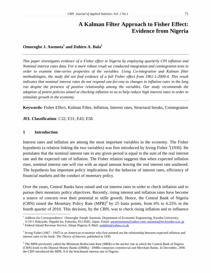
economic activities. Nigeria’s inflation rate has since moved from 13% in the second quarter to 13.7% in the third quarter of 2010 (CBN, 2010). Despite general acceptance of the Fisher hypothesis, empirical evidence has been difficult to establish even with massive literature generated from studying the relationship. While studies by Engsted (1995) and Hatemi-J (2008), among others, found no support for the hypothesis, Mishkin (1992), Evans and Lewis (1995), Wallace and Warner (1993), and Crowder and Hoffman (1996), finds evidence in favour of long-run Fisher effect. Cooray (2002), and Million (2003), reported weak and conflicting results. There are several reasons behind the inability to find evidence of a full Fisher effect. Tobin (1969) noted that investors re-balance their portfolios in favour of real assets during high inflationary periods. In addition, are the different types of interest rates and sample periods used in the empirical analysis. It may also be due to structural changes in the co-integrating vector. Mishkin (1986) noted that the relationship between interest rate and inflation, shift with changes in monetary policy regimes. A long-run Fisher effect implies that when interest rate is higher for a long period of time, the expected inflation rate will also tend to be high; this implies that the two variables are cointegrated; while a short-run effect indicates that a change in the interest rate is associated with an immediate change in the expected inflation rate (Mishkin, 1992).Interest rates affect the demand for and allocation of credits as well as the exchange and inflation rates. They also serve as incentive to savers.. Interest rates represent the cost of borrowing and return on deposits. They range from Monetary Policy Rates, Treasury bills, Deposit to Lending rates. Real interest rates are usually adjusted for changes in the price level while nominal rates are not adjusted and are usually equal to or greater than real interest rates. The divergence between the two rates is affected by inflation, risk, taxes, investment policy, and term to maturity (Uchendu, 1993). From Figure I, it can be observed that interest rates broadly move together from 1961-2009 in Nigeria. Interest rates were largely stable and moving together between 4-6%throughout 1960s to the late 1970s. The rates however showed substantial rise from 1980 to 1987 which was largely attributed to government’s policy of interest rates deregulation in the mid-1980s. They also witnessed high increments in 1993 with average interest rates hovering around 26%. The CBN made concerted efforts to reduce the rate in the mid-1990s, leading to a 13% drop in 2000. Policy rates declined further from2000 to 2007 despite noticeable divergence between the key interest rates compared to the pre-deregulation rates. Studies show that businesses consider interest rate an important factor in investment and would borrow at high rates of return if the investment would justify the high rates5. Similarly, Oresotu’s

5 Recently, the Central Bank of Nigeria (CBN) decided to make public on a weekly basis the average deposit and lending rates obtainable in all Deposit Money Banks (DMBs) to help guide business decisions in the economy. This decision took effect in 2010.


(1992) findings reveal that the key factor affecting nominal lending rate is persistent currency depreciation, through pressure on domestic liquidity.

Figure I: Short and long-term interest rates in Nigeria (1961-2009)

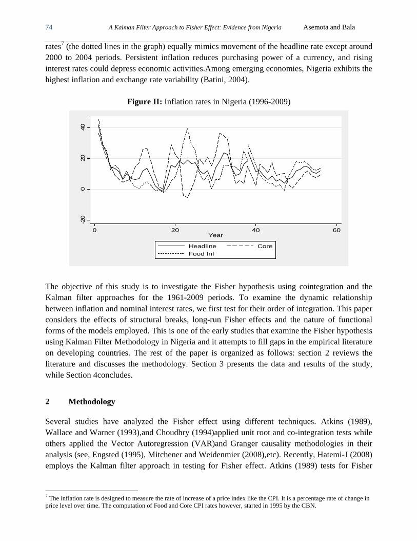
Presently, literature from developed countries on Fisher effect has concentrated on the dangers arising from either very low or high interest rates that include: a distorted allocation of capital, excessive risk-taking, and destabilizing surges in capital flows. The phenomenon of low and negative interest rates presents new challenges to monetary authorities in the US, the EU and Japan. Negative interest rate implies willingness to pay more for a bond today than will be received for it in the future6. Nigeria’s inflation experience since the mid-1990s has been mixed. This is depicted in Figure II which shows the plot of quarterly headline, food and core inflation rates for the last one and a half decades. The headline inflation rates (the solid line) stood at 41.9% in 1996:1, before witnessing substantial decline between 1997 and 1998. This reduction in inflation was due to tight monetary policy posture of the CBN in the mid-1990s. However, there were major increases in headline inflation to 13.55% in 1999:1 and a substantial drop to -1.43% in 2000:1. There were large increases between 2000 and 2002 with inflation rate hovering around 12.25% to19% respectively. A major decline was recorded around 2003:1 (5.8%) before rising substantially to 23.84% and 22.47% in 2003:4 and 2004:1. The inflation rate drops consistently from 2006:1 to 2008:1 and by mid-2008 the rates increased again (see figure 1). The core and food inflation 6 In October, 2009 the Bank of Japan (BOJ) cut its benchmark interest rate to almost zero percent in order to stimulate the economy. Rates had been held at 0.1% since the end of 2008. However, the BOJ earlier lifted the zero interest rate policy in July 2006. In late 1998, interest rates on Japanese six-month treasury bills became negative, yielding an interest rate of -0.004%, with investors paying more for the bills than their face value6 (Mishkin and Eakins, 2006, pp52).

010

2030

1960 1970 1980 1990 2000 2010YEAR

MPRATE T-BILLRT3MONTHS 6MONTHS12MONTHS OVER12MTS


rates7 (the dotted lines in the graph) equally mimics movement of the headline rate except around 2000 to 2004 periods. Persistent inflation reduces purchasing power of a currency, and rising interest rates could depress economic activities.Among emerging economies, Nigeria exhibits the highest inflation and exchange rate variability (Batini, 2004).

Figure II: Inflation rates in Nigeria (1996-2009)

The objective of this study is to investigate the Fisher hypothesis using cointegration and the Kalman filter approaches for the 1961-2009 periods. To examine the dynamic relationship between inflation and nominal interest rates, we first test for their order of integration. This paper considers the effects of structural breaks, long-run Fisher effects and the nature of functional forms of the models employed. This is one of the early studies that examine the Fisher hypothesis using Kalman Filter Methodology in Nigeria and it attempts to fill gaps in the empirical literature on developing countries. The rest of the paper is organized as follows: section 2 reviews the literature and discusses the methodology. Section 3 presents the data and results of the study, while Section 4concludes.

2 Methodology Several studies have analyzed the Fisher effect using different techniques. Atkins (1989), Wallace and Warner (1993),and Choudhry (1994)applied unit root and co-integration tests while others applied the Vector Autoregression (VAR)and Granger causality methodologies in their analysis (see, Engsted (1995), Mitchener and Weidenmier (2008),etc). Recently, Hatemi-J (2008) employs the Kalman filter approach in testing for Fisher effect. Atkins (1989) tests for Fisher

7 The inflation rate is designed to measure the rate of increase of a price index like the CPI. It is a percentage rate of change in price level over time. The computation of Food and Core CPI rates however, started in 1995 by the CBN.

-20

020

40

0 20 40 60Year

Headline CoreFood Inf


effect and found that post-tax nominal interest rates and inflation are co-integrated, and that interest rate influences changes in inflationary expectation set equilibrium. Mishkin (1992), in resolving the puzzle of why a strong Fisher effect occurs for some periods and not for others, identifies the lack of empirical evidence for a short-run Fisher effect to be due to the fact that a strong Fisher effect will only appear in samples where inflation and interest rates have stochastic trends. He claimed that empirical evidence finds no support for a short-run Fisher effect, but supports the existence of a long-run effect in which inflation and interest rates exhibit common trends. Wallace and Warner (1993) applied the expectations model of the term structure of interest rates to establish the conditions under which innovations in short-term inflation will be transmitted to short and long-term interest rates. Their co-integration test finds support for both the Fisher effect and the expectations theory of the term structure. Earlier, Sargent et al.(1973) incorporates rational expectations in their analysis of the Fisher model and finds several implications suggesting that real interest rate was independent of the systematic part of the money supply. However, they did not recommend the adoption of a systematic policy of pegging the nominal interest rate at some fixed level over many periods because such a policy would either be very inflationary or deflationary. Choudhry (1994) analyses the long-run interest-inflation relationships in the USA during the gold standard period (1879-1913) andhis results show that there exists Fisher effects on both the nominal short- and long-term interest rates. Mitchener and Weidenmier (2008) also got the same results with Choudhry (1994), in favour of the existence of Fisher effect in the USA during the same period. Engsted (1995) examines whether long-term interest rates predict future inflation by assuming the existence of rational expectations and constant ex-ante real rates and finds that for the sampled countries, inflation and interest rates may be regarded as non-stationary(1)I processes

that cointegrate to stationary spreads. Evans and Lewis (1995) noted that findings which suggest that nominal interest rate and expected inflation do not move together in the long run can be deceptive when the inflationary process shifts infrequently. They characterize the shifts in inflation by a Markov switching model but were unable to reject long-run Fisher effect. Mishkin and Simon (1995) examine the Fisher effect for Australia and finds weak evidence in support of the hypothesis. Their results indicate that while long-run Fisher effect seems to exist, there is no evidence of a short-run effect, since short-run changes in interest rates reflect changes in monetary policy, while long-run levels indicate inflationary expectations. Yuhn (1995) tests the relation for five countries and reveals that the Fisher effect was not robust to policy changes. His results indicate strong evidence of a long run Fisher effect except for the UK and Canada. However, short-run Fisher effect was only detected in Germany. Crowder and Hoffman (1996) argue that pre-tax nominal interest rates will not move one-for-one with inflation


in the long-run if real interest rates are supposed to be unaffected by permanent shocks to inflation. They suggested calculating variable marginal tax rates for the countries and testing the fisher effect with tax-adjusted interest rates. Darby (1975) equally incorporates tax into interest-inflation interactions. Hamori (1997) employs the Generalized Method of Moments (GMM) technique to test for Fisher effect using Japanese data from 1971–1994as this alternative approach makes it unnecessary to formulate the expected inflation rate explicitly as well as making it possible to simultaneously analyze the returns of multiple assets. Cooray (2002) surveys the literature by analyzing the techniques employed, as well as offering explanations for failure of the Fisher hypothesis. Cooray’s review finds that although studies for the US appear to suggest positive relationship between interest rates and inflation, they do not establish a one-to-one relationship as postulated by Fisher (1930). Million (2003) revisits the Fisher hypothesis, and attributes the inability of some empirical studies to recognize the Fisher effect to be due to errors in inflation expectations. Hatemi-J and Irandoust (2008) were also unable to find empirical support for a full Fisher effect using the Kalman filter algorithm. Their results were however consistent with many existing literature on the subject that found the estimated slope coefficients in the fisher equation to be less than the hypothesized value of one. Busari (2007) used the Hodrick and Prescott filter to analyse inflation into its trend, cyclical, seasonal and random components and finds that past behaviour of the trend component of inflation and money supply are the main determinants of long-run inflation in Nigeria. Marotta (2009) investigates whether size and speed of pass-through of market rates into short-term business lending rates have increased with the introduction of the Euro..His results were contrary to the intuition that a reduced volatility in money market rates is bound to mitigate uncertainty and to ease the transfer of policy rate changes to retail rates. Beyer et al. (2009) tests the long-run Fisher effect for 15 countries.. Their results reveal evidence of breaks in the cointegrating relationship for most of the countries studied. Though Beyer et al. finds support for cointegration between inflation and interest rates, the two variables do not move one-for-one in the long run for all cases. Ito (2009) examines the Fisher hypothesis in Japanese long-term interest rates by analyzing the asymmetric impacts of inflation expectations on interest rates. His co-integration test shows that all interest rates move together with expected inflation in long-run equilibrium. The implication of Ito’s result is that nominal interest rates in Japan were sensitive to inflationary expectations. Obi et al. (2009) investigates the existence of Fisher effect in Nigeria and confirm the existence of a long run partial Fisher effect from 1970-2007.

2.1 Unit root tests without a structural break

Prior to modeling our time series data, we determined the order of integration of the variables. The application of cointegration requires that time series data have the same stochastic structure.


If the order of integration of inflation rate is different from that of interest rate, the data becomes inconsistent with the cointegration procedure. The augmented Dickey-Fuller (ADF) test is the most applied statistical test for determining order of integration of macroeconomic time series. In the case of trending data, it is based on the following regression:

1

1

k

t t i t i ti

y t y d yµ β α ε− −=

∆ = + + + ∆ +∑ (1)

Where tε is a pure white noise error term and where1 1 2t t ty y y− − −∆ = − , 2 2 3t t ty y y− − −∆ = − , etc.

The lagged difference terms are added to make the error term well-behaved.8 Equation (1) tests the null hypothesis of a unit root against a trend stationary alternative. To achieve the most parsimonious model compatible with white-noise residuals, we selected k through the ‘tsig’ approach proposed by Hall (1994). This is a data dependent method that uses a general-to-specific recursive procedure based on the value of the t-statistic on the coefficient associated with the last lag in the estimated autoregression.9 Ng and Perron (1995) demonstrates through a simulation study that the ‘t sig’ approach is preferable to the information based criteria. For our quarterly data, we set the maximum number of lags ( )k to be equal to 12 (see Table 1 in the

Appendix).

2.2 Unit root tests with structural break

2.2.1 Zivot-Andrews unit root test

Perron (1989) demonstrates through a simulation experiment that the augmented Dickey-Fuller (hereafter, ADF) test is biased towards non-rejection of the unit root hypothesis if the data are characterized by stationary fluctuations around a trend function that exhibits a structural change. Perron’s methodology involves incorporation of dummy variables in the ADF test to account for one exogenous (known) structural break. The exogenous imposition of break date was criticized by Zivot-Andrews (hereafter, ZA) (1992). ZA (1992) proposes a data dependent algorithm to determine the breakpoint. Their unit root test procedure transforms Perron’s unit root test, which is conditional on a known breakpoint, into an unconditional unit- root test. Thus, following Perron’s ADF testing strategy, the ZA unit root test is carried out with the following regression equations:

Model A (Crash Model):

1

1

k

t t t i t i ti

y t DU y c yµ β θ α ε− −=

= + + + + ∆ +∑

(2)

8 In statistical parlance, the error term is said to be well-behaved when it is independently and identically normally distributed. 9 This procedure involves starting with a predetermined maximum k say kmax, if kmax is significant, it is chosen. Else, it is reduced by one recursively, until the last lag become significant. However, k is set equal to zero if no lags are significant.


Model B (Changing Growth Model):

1

1

k

t t t i t i ti

y t DT y c yµ β γ α ε− −=

= + + + + ∆ +∑

(3)

Model C (Mixed Model):

11

k

t t t t i t i ti

y t DU DT y c yµ β θ γ α ε− −=

= + + + + + ∆ +∑

(4)

Where 1tDU = if ,t TB> 0 otherwise; tDT t TB= − if ,t TB> 0 otherwise, TB is the date of the

endogenously determined break. Model A, referred to as the “crash model” allows for a one-time change in the intercept of the trend function, model B, referred to as the “changing growth model” allows for a single change in the slope of the trend function without any change in the level; and model C, the “mixed model” allows for both effects to take place simultaneously, i.e., a sudden change in the level followed by a different growth path.10 The null hypothesis for the three models is that the series is integrated (unit root) without structural breaks (α = 1). The test statistic is the minimum “t ” over all possible break dates in the sample. ZA (1992) suggested using a trimming region of (0.10T, 0.90T) to eliminate endpoints. The k extra regressors in the preceding regressions are determined by the ‘t sig’ approach proposed by Hall (1994).

2.2.2 Perron (1997) Unit root test with a structural break

The ZA unit root test only allows for structural break in the null hypothesis, this omits the possibility of a unit root with structural break.11Due to criticism of the Perron (1989) exogenous (known) break test by Zivot-Andrews (1992) and Christiano (1992)12, Perron (1997) re-visits this issue and proposes an endogenous one-break unit root test where the break point is perfectly correlated with the data and the structural break is included in both the null and alternative hypotheses. We consider the innovational outlier model that allows for change in the intercept

10 In our empirical analysis, we report results of model A and model C because Perron (1989) suggests that most macroeconomic time series can be adequately modeled using either model A or model C. In addition, Sen (2003) argued that if one assumes that the location of the break is unknown, it is most likely that the form of the break will be unknown as well. Sen (2003) assesses the performance of the minimum t statistics when the form of the break is mis-specified. His simulation experiment revealed that the loss in power is quite negligible if the mixed model specification is used when in fact that the break occurs according to the crash model or changing growth model, and concluded that practitioners should specify the mixed model in empirical applications. 11Perron (1989) allows for structural break under the null and alternative hypothesis. Lee and Strazicich (2004) noted that if a break exists under the null, undesirable results will inevitably occur. The ZA unit root test will exhibit size distortions leading to spurious rejections of the unit root null hypothesis. Hence, researchers may incorrectly conclude that a series is stationary with break when in fact the series is nonstationary with break. 12 Christian (1992) argued that the choice of the break date to a large extent has to be viewed as being correlated with the data. This is important because both the finite sample and asymptotic distributions of the test statistics depend upon the extent of correlation between the break point and data.


and the slope of the trend function to take place gradually.13 In model A (Crash Model), unit root test is performed using the t -statistic for testing = 1α in the following regression:

Model A:

11

( )k

t t b t t i t i ti

y DU t dD T y c yµ θ β α ε− −=

= + + + + + ∆ +∑ (5)

Where 1tDU = , if bt T> (0 otherwise), ( ) 1,b tD T = if 1t Tb= + (0 otherwise), andbT is the time of the

structural break. The above regression is estimated by OLS and it is in the spirit of the Dickey-Fuller test (1979) and Said and Dickey (1984) methodology, whereby autoregressive moving average (ARMA) processes are approximated by autoregressive processes. For Model C, the test is performed, the t -statistic for testing = 1α in the following regression:

Model C:

1

1

( )k

t t t b t t i t i ti

y DU t DT dD T y c yµ θ β γ α ε− −=

= + + + + + + ∆ +∑ (6)

( ) if 0 otherwise .t bDT t t T= > Perron (1997) noted that selecting Tb based on the parameter of

the change in intercept or slope is likely to allow tests with greater power. We followed this recommendation in our empirical analysis.

2.3 Cointegration Analysis

2.3.1 Cointegration without structural break

If the interest rate (denoted bytN ) and inflation rate (denoted bytF ) are both integrated of order 1,

they are said to be cointegrated if a linear combination of them is integrated of order zero. Statistically, tN and tF are cointegrated, if both are(1)I and if tε is (0)I in the following

cointegrating regression:

= + + t t tN Fα β ε (7)

Cointegration tests are carried out using the Engle and Granger (1987) two-step estimation procedure14. The procedure involves estimating the cointegrating regression equation above using Ordinary Least Squares (OLS) and then conducting unit root tests for the residualsˆtε . Long-run

Fisher effect implies that interest rates and inflation are cointegrated. Enders (1996) noted that the Engle and Granger (hereafter, EG) procedure, though can be easily implemented, have some

13 The additive outlier model assumes that the change to the series occurs instantaneously, which may be a poor description of the data generating process. 14Co-integration is a concept that captures the co-movements of variables towards long-run equilibrium.


limitations. The two-step procedure can lead to multiplicity of errors; any error generated in the first step is automatically transferred to the second stage. In addition, the technique requires specifying the dependent and explanatory variables. In practice, it may be possible to find that one regression indicates that the variables are cointegrated; however, reversing the order indicates no cointegration. Again, the test is deficient when there are three or more variables; hence, there may be more than one cointegrating vector. To circumvent these inherent problems of the EG test; we supplemented the estimation of the cointegration relationship with Johansen (1988) Maximum-Likelihood Estimators. The Johansen cointegration test circumvents the use of two-step estimators, it is also invariant to the choice of variable selected for normalization and can estimate and test for the presence of multiple cointegrating vectors. For description of this procedure, see Johansen (1988).

2.3.2 Cointegration with structural break

The EG and Johansen traditional tests have limitations especially when dealing with a long data span that may have been affected by major economic events such as policy changes, economic, financial or energy crises. Gregory, Nason, and Watt (1996) demonstrate that the power of the ADF based cointegration tests fall sharply in the presence of a structural break (intercept shift). Gregory and Hansen (1996) argue that if a model is cointegrated with a one-time regime shift in the cointegrating vector, the traditional tests discussed in section 2.2.2 may not reject the null and the researcher may falsely conclude that there is no long-run relationship. To obtain robust cointegration results, we also apply the Gregory and Hansen (1996) cointegration test that allows the cointegrating vectors to change at a single unknown time during the sample period. The null hypothesis (no cointegration) is the same with the conventional test, and the alternative is cointegration with structural break. Kasman and Ayhan (2008) noted that the Gregory and Hansen (hereafter, GH) test could especially be insightful when the null hypothesis of no cointegration is not rejected by the conventional tests. GH (1996) estimated three models; the level shift model denoted by C, the second model the level shift with trend (C/T); introduce a time trend into the level shift model and the third model regime shift allows the slope vector and the intercept to change. The three models are given by the following regression equations:

Model 1: Level shift (C)

1 1 2 2 + + + , 1, , . Tt t t ty y e t nτµ µ ϕ α= = K (8)

where 1µ represents the intercept before the shift, and 2µ represents the change in the intercept at

the time of the shift. 1ty and 2ty are integrated variables of order 1.

Model 2: Level shift with trend ( /C T )

1 1 2 2 + + + , 1, , . Tt t t ty t y e t nτµ µ ϕ β α= + = K

(9)

Wheret denotes the time trend.


Model 3: Regime shift ( /C S )

1 1 2 1 2 2 2 + + + , 1, , .T Tt t t t t ty y y e t nτ τµ µ ϕ α α ϕ= + = K

(10)

in this case, 1µ and 2µ are as in model 1, 1α denotes the cointegrating slope coefficients before

the regime shift, and 2α denotes change in the slope coefficients. The dummy variable that

captures structural change is given by:

[ ][ ]

0 =

1 t

if t n

if t nτ

τϕ

τ ≤ > (11)

Where the unknown parameter (0,1)τ ∈ denotes the relative timing of the change point, and [ ]

denotes integer part. The cointegration test statistic for each possible regime shift Tτ ∈ is the smallest value (the largest negative values i.e., the value that provides the strongest evidence against the null hypothesis) across all possible break points. GH (1996) suggests computing the test statistic for each break point in the interval ([0.15n], [0.85n]).

2.4. The Kalman Filter (KF)

The cointegrating regression equation (7) specified in section 2.2.2 assumes that the slope coefficient is constant throughout the data span. Hence, it does not allow the parameter to change across time. This specification may be highly deficient especially in economic and business applications where the level of randomness is high, and also where the constancy of patterns or parameters cannot be guaranteed. Thus, a more flexible model is the time-varying parameter model; it allows the slope parameter to vary randomly across time. In statistical arena, this flexible model is popularly referred to as the state space model. The state space representation of equation (7) is given by:

1

= +

= + t t t t

t t t

N Fα β εβ β η−

+

(12)

The first equation in 12 is called the observation equation or measurement equation while the second is the state or transition equation. The measurement equation relates the observed variables (data) and the unobserved state variable ( tβ ), while the transition equation describes the

evolution of the state variable. The observation error tε and state error tη are assumed to be

Gaussian white noise (GWN) sequences. The overall objective of state space analysis is to study the development of the state (tβ ) over time using observed data. When a model is cast in a state

space form, the Kalman filter is applied to make statistical inference about the model15. The

15The Kalman Filter is a computationally efficient method of updating the estimates of the time-dependent parameters of a multiple regression model as successive values of the dependent variable become available. Exponential smoothing provides an extremely simple example of the recursive calculations involved. The procedure was introduced by Kalman, Rudolf Emil in 1960( see Upton, G and Cook, I (2008)).

82 A Kalman Filter Approach to Fisher Effect: Evidence from Nigeria

Kalman filter (hereafter, KF) is simply a recursive statistical algorithm for carrying out computations in a state space model. A more accurate estimate of the state vector or slope

coefficient can be obtained via Kalman Smoothing (K.S). The unknown variance parameters (

and 2ησ ) in model 12 are estimated by the maximum likelihood estimation via the Kalman filter

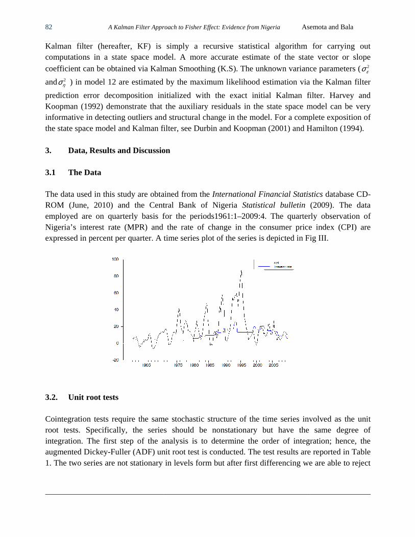
prediction error decomposition initialized with the exact initial Kalman filter. Harvey and Koopman (1992) demonstrate that the auxiliary residuals in the state space model can be very informative in detecting outliers and structural change in the model. For a complete expositionthe state space model and Kalman filter, see Durbin and Koopman (2001) and Hamilton (1994). 3. Data, Results and Discussion 3.1 The Data The data used in this study are obtained from the ROM (June, 2010) and the Central Bank of Nigeria employed are on quarterly basis for the periods1961:1Nigeria’s interest rate (MPR) and the rate of change in the consuexpressed in percent per quarter. A time series plot of the series is depicted in Fig III.

3.2. Unit root tests Cointegration tests require the same stochastic structure of the time series involved as the unit root tests. Specifically, the series should be nonstationary but have the same degree of integration. The first step of the analysis is to determine the order of integration; hence, the augmented Dickey-Fuller (ADF) unit root test is conducted. The test results are repor1. The two series are not stationary in levels form but after first differencing we are able to reject

A Kalman Filter Approach to Fisher Effect: Evidence from Nigeria Asemota and Bala


oefficient can be obtained via Kalman Smoothing (K.S). The unknown variance parameters (

) in model 12 are estimated by the maximum likelihood estimation via the Kalman filter

sition initialized with the exact initial Kalman filter. Harvey and Koopman (1992) demonstrate that the auxiliary residuals in the state space model can be very informative in detecting outliers and structural change in the model. For a complete expositionthe state space model and Kalman filter, see Durbin and Koopman (2001) and Hamilton (1994).

Data, Results and Discussion

obtained from the International Financial StatisticsROM (June, 2010) and the Central Bank of Nigeria Statistical bulletin employed are on quarterly basis for the periods1961:1–2009:4. The quarterly observation ofNigeria’s interest rate (MPR) and the rate of change in the consumer price index (CPI) are expressed in percent per quarter. A time series plot of the series is depicted in Fig III.

the same stochastic structure of the time series involved as the unit cifically, the series should be nonstationary but have the same degree of

integration. The first step of the analysis is to determine the order of integration; hence, the Fuller (ADF) unit root test is conducted. The test results are repor

1. The two series are not stationary in levels form but after first differencing we are able to reject

Asemota and Bala


oefficient can be obtained via Kalman Smoothing (K.S). The unknown variance parameters (2εσ

) in model 12 are estimated by the maximum likelihood estimation via the Kalman filter

sition initialized with the exact initial Kalman filter. Harvey and Koopman (1992) demonstrate that the auxiliary residuals in the state space model can be very informative in detecting outliers and structural change in the model. For a complete exposition of the state space model and Kalman filter, see Durbin and Koopman (2001) and Hamilton (1994).

International Financial Statistics database CD-Statistical bulletin (2009). The data 2009:4. The quarterly observation of

mer price index (CPI) are expressed in percent per quarter. A time series plot of the series is depicted in Fig III.

the same stochastic structure of the time series involved as the unit cifically, the series should be nonstationary but have the same degree of

integration. The first step of the analysis is to determine the order of integration; hence, the Fuller (ADF) unit root test is conducted. The test results are reported in Table

1. The two series are not stationary in levels form but after first differencing we are able to reject


the unit root null hypothesis with or without trend. This implies that the nonstationary series are integrated of order 1.

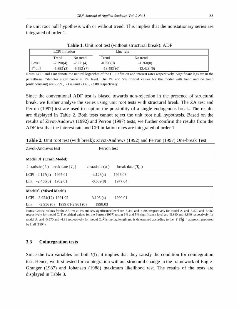
Table 1. Unit root test (without structural break): ADF LCPI Inflation Lint rate

Trend No trend Trend No trend

Level -2.290(4) -2.271(4) -0.705(0) -1.360(0)

1st diff -5.883∗(3) -5.592∗(7) -13.483∗(0) -13.428∗(0)

Notes:LCPI and Lint denote the natural logarithm of the CPI inflation and interest rates respectively. Significant lags are in the

parenthesis. ∗denotes significance at 1% level. The 1% and 5% critical values for the model with trend and no trend (only constant) are -3.99 , -3.43 and -3.46 , -2.88 respectively.

Since the conventional ADF test is biased towards non-rejection in the presence of structural break, we further analyse the series using unit root tests with structural break. The ZA test and Perron (1997) test are used to capture the possibility of a single endogenous break. The results are displayed in Table 2. Both tests cannot reject the unit root null hypothesis. Based on the results of Zivot-Andrews (1992) and Perron (1997) tests, we further confirm the results from the ADF test that the interest rate and CPI inflation rates are integrated of order 1. Table 2. Unit root test (with break): Zivot-Andrews (1992) and Perron (1997) One-break Test

Zivot-Andrews test Perron test

Model A (Crash Model)

t -statistic (k ) break-date (bT ) t -statistic (k ) break-date (bT )

LCPI -4.147(4) 1997:01 -4.128(4) 1996:03

Lint -2.458(0) 1982:01 -0.509(8) 1977:04

Model C (Mixed Model)

LCPI -3.924(12) 1991:02 -3.106 (4) 1990:01

Lint -2.956 (0) 1999:01-2.961 (0) 1998:03

Notes: Critical values for the ZA test at 1% and 5% significance level are -5.340 and -4.800 respectively for model A, and -5.570 and -5.080 respectively for model C. The critical values for the Perron (1997) test at 1% and 5% significance level are -5.340 and-4.840 respectively for

model A, and -5.570 and -4.91 respectively for model C. k is the lag length and is determined according to the ‘ t sig ’ approach proposed

by Hall (1994).

3.3 Cointegration tests Since the two variables are both(1)I , it implies that they satisfy the condition for cointegration

test. Hence, we first tested for cointegration without structural change in the framework of Engle-Granger (1987) and Johansen (1988) maximum likelihood test. The results of the tests are displayed in Table 3.


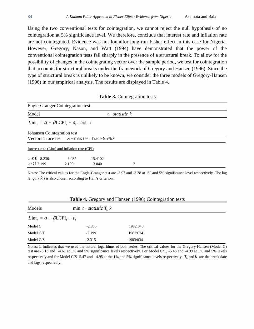
Using the two conventional tests for cointegration, we cannot reject the null hypothesis of no cointegration at 5% significance level. We therefore, conclude that interest rate and inflation rate are not cointegrated. Evidence was not foundfor long-run Fisher effect in this case for Nigeria. However, Gregory, Nason, and Watt (1994) have demonstrated that the power of the conventional cointegration tests fall sharply in the presence of a structural break. To allow for the possibility of changes in the cointegrating vector over the sample period, we test for cointegration that accounts for structural breaks under the framework of Gregory and Hansen (1996). Since the type of structural break is unlikely to be known, we consider the three models of Gregory-Hansen (1996) in our empirical analysis. The results are displayed in Table 4.

Table 3. Cointegration tests

Engle-Granger Cointegration test

Model t statistic− k

int = + LCPI + t t tL α β ε -1.045 4

Johansen Cointegration test Vectors Trace test maxλ − test Trace-95%k Interest rate (Lint) and inflation rate (CPI)

0r ≤ 8.236 6.037 15.4102 1r ≤ 2.199 2.199 3.840 2

Notes: The critical values for the Engle-Granger test are -3.97 and -3.38 at 1% and 5% significance level respectively. The lag length (k ) is also chosen according to Hall’s criterion.

Table 4. Gregory and Hansen (1996) Cointegration tests

Models min t statistic− bT k

int = + LCPI + t t tL α β ε

Model C -2.866 1982:040

Model C/T -2.199 1983:034

Model C/S -2.315 1983:034

Notes: L indicates that we used the natural logarithms of both series. The critical values for the Gregory-Hansen (Model C) test are -5.13 and -4.61 at 1% and 5% significance levels respectively. For Model C/T, -5.45 and -4.99 at 1% and 5% levels

respectively and for Model C/S -5.47 and -4.95 at the 1% and 5% significance levels respectively. bT andk are the break date

and lags respectively.


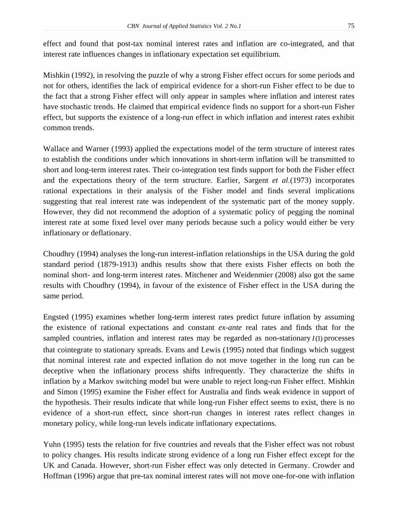
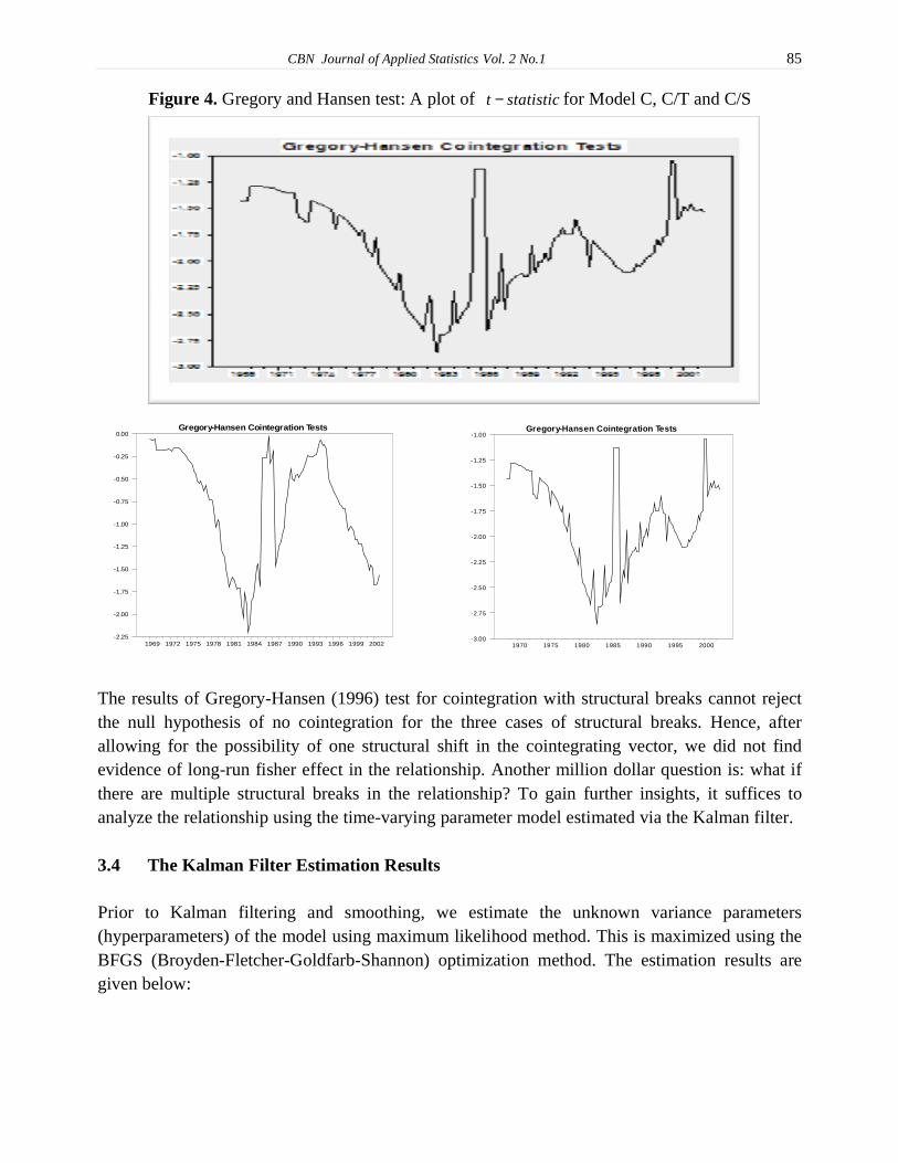
Figure 4. Gregory and Hansen test: A plot of t statistic− for Model C, C/T and C/S

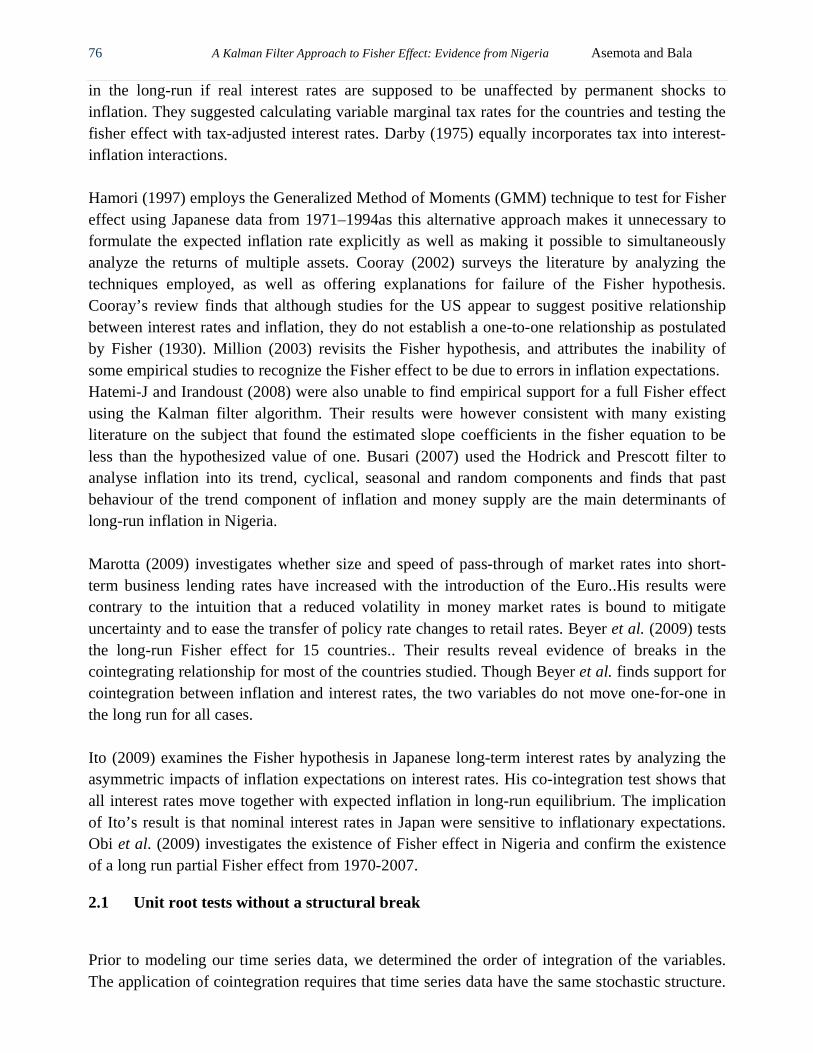
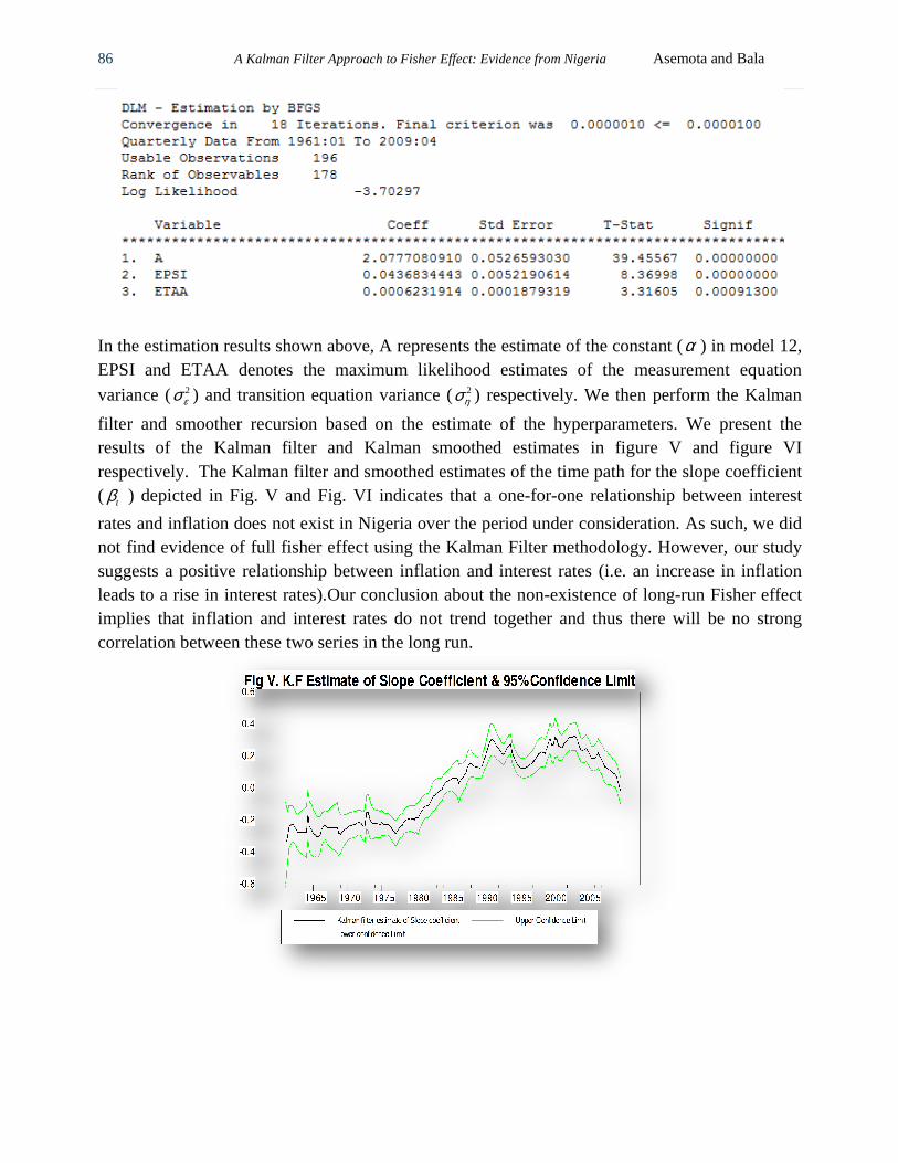
The results of Gregory-Hansen (1996) test for cointegration with structural breaks cannot reject the null hypothesis of no cointegration for the three cases of structural breaks. Hence, after allowing for the possibility of one structural shift in the cointegrating vector, we did not find evidence of long-run fisher effect in the relationship. Another million dollar question is: what if there are multiple structural breaks in the relationship? To gain further insights, it suffices to analyze the relationship using the time-varying parameter model estimated via the Kalman filter. 3.4 The Kalman Filter Estimation Results Prior to Kalman filtering and smoothing, we estimate the unknown variance parameters (hyperparameters) of the model using maximum likelihood method. This is maximized using the BFGS (Broyden-Fletcher-Goldfarb-Shannon) optimization method. The estimation results are given below:

Gregory-Hansen Cointegration Tests

1969 1972 1975 1978 1981 1984 1987 1990 1993 1996 1999 2002-2.25

-2.00

-1.75

-1.50

-1.25

-1.00

-0.75

-0.50

-0.25

0.00Gregory-Hansen Cointegration Tests

1970 1975 1980 1985 1990 1995 2000-3.00

-2.75

-2.50

-2.25

-2.00

-1.75

-1.50

-1.25

-1.00

86 A Kalman Filter Approach to Fisher Effect: Evidence from Nigeria

In the estimation results shown above, A represents the estimate of the constant (EPSI and ETAA denotes the maximum likelihood estimates of the measurement equation

variance ( 2εσ ) and transition equation varian

filter and smoother recursion based on the estimate of the hyperparameters. We present the results of the Kalman filter and Kalman smoothed estimates in figure V and figure VI respectively. The Kalman filter and smoothed estimates of the time path for the slope coefficient ( tβ ) depicted in Fig. V and Fig. VI indicates that a one

rates and inflation does not exist in Nigerinot find evidence of full fisher effect using the Kalman Filter methodology. However, our study suggests a positive relationship between inflation and interest rates (i.e. an increase in inflation leads to a rise in interest rates).Our conclusion about the nonimplies that inflation and interest rates do not trend together and thus there will be no strong correlation between these two series in the long run.

A Kalman Filter Approach to Fisher Effect: Evidence from Nigeria Asemota and Bala

results shown above, A represents the estimate of the constant (EPSI and ETAA denotes the maximum likelihood estimates of the measurement equation

) and transition equation variance ( 2ησ ) respectively. We then perform the Kalman

filter and smoother recursion based on the estimate of the hyperparameters. We present the results of the Kalman filter and Kalman smoothed estimates in figure V and figure VI

ively. The Kalman filter and smoothed estimates of the time path for the slope coefficient ) depicted in Fig. V and Fig. VI indicates that a one-for-one relationship between interest

rates and inflation does not exist in Nigeria over the period under consideration. As such, we did not find evidence of full fisher effect using the Kalman Filter methodology. However, our study suggests a positive relationship between inflation and interest rates (i.e. an increase in inflation

s to a rise in interest rates).Our conclusion about the non-existence of longimplies that inflation and interest rates do not trend together and thus there will be no strong correlation between these two series in the long run.

Asemota and Bala

results shown above, A represents the estimate of the constant (α ) in model 12, EPSI and ETAA denotes the maximum likelihood estimates of the measurement equation

) respectively. We then perform the Kalman

filter and smoother recursion based on the estimate of the hyperparameters. We present the results of the Kalman filter and Kalman smoothed estimates in figure V and figure VI

ively. The Kalman filter and smoothed estimates of the time path for the slope coefficient one relationship between interest

a over the period under consideration. As such, we did not find evidence of full fisher effect using the Kalman Filter methodology. However, our study suggests a positive relationship between inflation and interest rates (i.e. an increase in inflation

existence of long-run Fisher effect implies that inflation and interest rates do not trend together and thus there will be no strong

CBN Journal of Applied Statistics

We further consider the possibility of outliers and structural breaks in our timemodel using the framework of Harvey and Koopmanauxiliary residuals in state space models are useful tools for detestate space model. The detection procedure is to plot the standardized residuals. Since the model is Gaussian, indications of outliers and structural breaks arise for values greater than 2 in absolute value. We plot the standardized auxiliary residuals in Fig VII. The plots of the residuals indicate the presence of outliers in the inflation

Journal of Applied Statistics Vol. 2 No.1

We further consider the possibility of outliers and structural breaks in our time-varying parameter model using the framework of Harvey and Koopman (1992). The duo demonstrates that the auxiliary residuals in state space models are useful tools for detecting outliers and shifts in the state space model. The detection procedure is to plot the standardized residuals. Since the model is Gaussian, indications of outliers and structural breaks arise for values greater than 2 in absolute

ndardized auxiliary residuals in Fig VII. The plots of the residuals indicate the presence of outliers in the inflation-interest rates relationship in 1964, 1973, 1991 and 2000.

87

varying parameter (1992). The duo demonstrates that the

cting outliers and shifts in the state space model. The detection procedure is to plot the standardized residuals. Since the model is Gaussian, indications of outliers and structural breaks arise for values greater than 2 in absolute

ndardized auxiliary residuals in Fig VII. The plots of the residuals indicate interest rates relationship in 1964, 1973, 1991 and 2000.


We find strong evidence of structural breaks in the relationship in 1990 and 1994, and weak evidence of structural break around 2008. 4 Conclusion This paper tests the existence of Fisher effect in Nigeria. Employing unit root tests, co-integration analysis, and the Kalman filter algorithm, we did not find evidence of a long-run Fisher effect from 1961-2009. This is consistent with majority of existing literature on the hypothesis. The results of our unit root tests show that interest rates (MPR) and CPI inflation are integrated of order 1, while the co-integration analysis shows that the two variables are not co-integrated. This article, apart from employing a more flexible time-varying parameter model which allows the slope parameter to vary randomly across time, utilizes the longest available quarterly inflation and interest rate series. Therefore, after allowing for the possibility of one structural shift in the co-integrating vector, we did not find evidence of a long-run Fisher effect in the relationship. Our study recommends the adoption of potent policies by the monetary authorities aimed at checking inflation so as to help reduce high interest rates in order to stimulate growth in the economy. ACKNOWLEDGEMENTS

The first author appreciates the financial support of the Japanese government through the Ministry of Education, Culture, Sports, Science and Technology (MEXT) of Japan. While the second author thank Mohammed Bala Audu, Nura Dauran, Bashua Saeed and Immam Shuaibu, for valuable comments and suggestions.

References Atkins, F.J.(1989).“Co-integration, Error Correction and the Fisher Effect”, Applied Economics, 21:1611 – 1620. Batini, N. (2004).“Achieving and Maintaining Price Stability in Nigeria”, International Monetary Fund Working Paper 0497. Beyer, A., Haug, A.A. and Dewald, W.G.(2009).“Structural Breaks, Co-integration and the Fisher Effect”, European Central Bank Working Paper Series, No. 1013 Busari, D.T. (2007). “On the Determinants of Inflation in Nigeria:1980-2003”.CBN Economic and Financial Review, 45:35-55. Central Bank of Nigeria(2010).Statistical Bulletin, 50 years Special Anniversary Edition, Abuja.

Choudhry, T. (1996).“The Fisher Effect and the Gold Standard: evidence from the USA”, Applied Economic letters,3:553-555.

Christiano, L.(1992).“Searching for a Break in GNP”, Journal of Business and Economic

Statistics, 10:237-250.


Cooray, A. (2002).“The Fisher Effect: A Review of the Literature”, Research papers 0206, Macquarie University, Department of Economics. Crowder, W.J. and Hoffman, D.L.(1996).“The Long-Run Relationship between Nominal Interest

Rates and Inflation: The Fisher Equation Revisited”, Journal of Money, Credit and Banking, 28(1):102 – 118.

Darby, M.R. (1975). “The Financial and Tax Effects of Monetary policy on Interest Rates,

Economic Inquiry, 12: 266-276. Dickey, D. and Fuller, W.A. (1979).“Distribution of the estimators for autoregressive time series with a unit root”, Journal of the American Statistical Association, 74: 427-431. Durbin, J. and Koopman, S.(2001).Time Series Analysis by State Space Methods, Oxford, Oxford University Press. Enders, W. (1996).RATS Handbook for Econometric Time Series, New York: John Wiley and

Sons Inc. Engle, R.F. and Granger, C.W.J.(1987). “Co-integration and Error Correction: Representation, Estimation, and Testing”, Econometrica, 55(2):251-276. Engsted, T.(1995).“Does the Long-Term Interest Rate Predict Future Inflation? A Multi-Country Analysis”, The Review of Economics and Statistics,77(1):42-54. Evans, M.D.D. and Lewis, K.K.(1995).“Do Expected Shifts in Inflation Affect Estimates of Long-Run Fisher Relation?”,The Journal of Finance,50, (1):225 – 253. Fisher, Irving (1930). The Theory of Interest. New York: Macmillan. Gregory, A.W. and Hansen, B.E. (1996).“Residual-based tests for Cointegration in Models with

Regime Shifts”, Journal of Econometrics,70: 99-126. Gregory, A.W., Nason, J.M. and Watt, D.(1996).“Testing for Structural Breaks in Cointegrated

Relationships”, Journal of Econometrics, 71:321-341. Hall, A.D.(1994).“Testing for a unit root in time series with pretest data based model selection”,

Journal of Business and Economic Statistics, 12:461-470. Hamilton, J.D. (1994).Time Series Analysis, Princeton University Press, New Jersey. Hamori, S.(1996).“A simple method to test the Fisher effect”, Applied Economics Letters, 4:477 - 479. Harvey, A.C. and Koopman, S.J.(1992).“Diagnostic Checking of Unobserved Components

Time Series Models”, Journal of Business and Economics Statistics,10(4):377-389. Hatemi-J, A.(2002). “Is the Government’s Inter-temporal budget constraint fulfilled in Sweden?


An application of the Kalman filter”, Applied Economics Letters, 9:433-439. Hatemi-J, A. and Irandoust, M.(2008).“The Fisher Effect: A Kalman Filter Approach to Detecting Structural change”, Applied Economics Letters,15:619-624. Ito, T.(2009).“Fisher Hypothesis in Japan: Analysis of long-term interest rates under different Monetary Policy Regimes”, The World Economy. Johansen, S.(1988). “Statistical Analysis of Cointegration Vectors”, Journal of Economic

Dynamics and Control 12:231-254. Kasman, A. and Ayhan, D.(2008).“Foreign Exchange Reserves and Exchange rates in Turkey:

Structural Breaks, Unit Roots and Cointegration”, Economic modeling, 25:83-92. Lee, J and Strazicich, M.C (2004). “Minimum LM test with one structural break”, Department of

Economics, Appalachian State University. Marotta, G.(2009).“Structural Breaks in the lending Interest rate Pass-through and the Euro”, Economic Modeling, 26:191-205. Million, N.(2003).“The Fisher Effect revisited through an Efficient non-linear unit root testing Procedure”, Applied Economic Letters, 10:951-954. Mishkin, F.S.(1992).“Is the Fisher effect for real? A re-examination of the Relationship between Inflation and interest rates”, Journal of Monetary Economics, 30:195 – 215. Mishkin, F.S.and Simon, J.(1995).“An empirical examination of the Fisher effect in Australia”, NBER Working Paper Series No.5080. Mishkin, F. S. and Eakins, S.G.(2006).Financial Markets and Institutions, Fifth Edition, Pearson International Edition, Addison Wesley, Boston. Mitchener, K.J. and Weidenmier, M.D.(2008).“Searching for Irving Fisher”, National Bureau Of Economic Research (NBER) Working Paper Ng, S. and Perron, P. (1995).“Unit root tests in ARMA models with data dependent methods for

Selection of the truncation lag”,Journalof American Statistical Association, 90: 268-281. Obi, B.,Nurudeen, A., and Wafure, O.B. (2009). “An Empirical Investigation of the Fisher Effect

in Nigeria: A Cointegration and Error Correction Approach”. International Review of Business Research Papers, 5: 96-109.

Oresotu (1992). “Interest rates Behavior under a Programme of Financial Reform: The Nigerian

Case”.CBN Economic and Financial Review, 30(2):109-125. Perron, P.(1989).“The great crash, the oil price shock and the unit root hypothesis”,

Econometrica,57:1361-1401.


Perron, P. (1997).“Further Evidence on Breaking trend functions in macroeconomic variables”, Journal of Econometrics, 80:355-385.

Phillips, P.C.B. and Perron, P. (1988). “Testing for a Unit Root in Time Series Regression”, Biometrika, 75:335-346. Said, S. and Dickey, D. (1984). “Testing for Unit Roots in Autoregressive Moving Average Models with Unknown Order”, Biometrica, 71:599-607. Sargent, T.J., Fand, D and Goldfeld, S.(1973).“Rational Expectations, the Real Rate of Interest,

And the Natural Rate of Unemployment”, Brookings Papers on Economic Activity, 2:429-480.

Sen, A.(2003). “On unit root tests when the alternative is a trend-break stationary process”,

Journal of Business and Economic Statistics,21(1):174-184. Uchendu, O.A.(1993).“Interest Rate Policy, Savings and Investment in Nigeria”, Central Bank of Nigeria Economic and Financial Review, 31(1):34-52. Upton, G and Cook, I. (2008). “A Dictionary of Statistics”, Oxford University Press, Oxford,

UK. pp 199. Wallace, M.S. and Warner, J.T.(1993).“The Fisher Effect and the term Structure of Interest Rates: Tests of Co-integration”, The Review of Economics and Statistics,75,(2):320-324. Yuhn, K.(1996). “Is the Fisher effect robust? Further evidence”, Applied Economics letters, 3:41-44. Zivot, E. and Andrews, D.W.K.(1992).“Further evidence on the Great Crash, the Oil-price

Shock, and the Unit Root Hypothesis”, Journal of Business and Economic Statistics, 10(3): 251-270.

a kalman filter approach to fisher effect: evidence from

Documents