a joint optimization model of ðs inventory and supply

Research ArticleA Joint Optimization Model of ðs, SÞ Inventory and SupplyStrategy Using an Improved PSO-Based Algorithm

Huayang Deng, Quan Shi , and Yadong Wang

Army Engineering University, Shijiazhuang Campus, Shijiazhuang, Hebei 050003, China

Correspondence should be addressed to Quan Shi; [email protected]

Received 9 July 2021; Revised 10 August 2021; Accepted 12 August 2021; Published 31 August 2021

Academic Editor: Thippa Reddy G

Copyright © 2021 Huayang Deng et al. This is an open access article distributed under the Creative Commons Attribution License,which permits unrestricted use, distribution, and reproduction in any medium, provided the original work is properly cited.

This paper mainly discussed the problem of a multiechelon and multiperiod joint policy of inventory and supply network.According to the random lead time and customers’ inventory demand, the ðs, SÞ policy was improved. Based on themultiechelon supply network and the improved, the dynasty joint model was built. The supply scheme in every periodwith the objective of minimum total costs is obtained. Considering the complexity of the model, the improved particleswarm optimization algorithm combining the adaptive inertia weight and grading penalty function is adopted to calculatethis model and optimize the spare part problems in various environments.

1. Introduction

As an important foundation of product maintenance, theresearch on spare parts in product maintenance is increas-ingly applied in industrial and military fields. Along withmore and more research, it becomes more and more mature.

In the last practice, many researchers have studied manyaspects in every field of spare parts. Sherbrooke in the estab-lishment of the aviation spare for maximum availability con-sidered the failure laws of a complex system and establisheda spare part demand model under complex factors [1]. Huet al. analyzed the characteristics of various spare part inven-tory policies and distinguished the best use conditions fordifferent inventory policies [2]. Ghobbar and Friend addeddynamic coordination to the study of multistage spare partsupply to improve the stability of the spare part supply pro-cess and improve system efficiency [3].

With the deepening of the research, the research of sparepart work is not limited to one aspect and gradually beginsto deepen the research on the whole process of spare partwork. Among these, the researchers are more interested inthe joint optimization of spare part inventory and supply pro-cess. In the study of joint optimization, it is resulting from theflexibility and random factors of maintenance mode, to con-

sider multiperiod continuous process than to study spare partstrategy for a certain period which is more valuable.

In the research of inventory policy, considering the char-acteristics of modern inventory, then the ðT , SÞ and ðs, SÞ pol-icies are more in line with the actual inventory managementexperience [4]. According to the ðT , SÞ policy, the capacity willbe replenished to S in the same time interval of time T [5]. Asfor the ðs, SÞ policy, when the capacity decreases less than s, thecapacity is replenished whose capacity maximum is S. In con-trast, the ðs, SÞ policy is more flexible and more complex in theresearch of inventory policy so that the joint inventory policyis less studied. This paper will make use of the characteristicsand advantages of the ðs, SÞ policy in joint optimization tocarry out joint optimization research [6].

In the project of joint optimization of inventory and supply,researchers focus on balancing transportation costs and break-down losses caused by insufficient inventory based on satisfy-ing demand and then determining the supply lead time, toachieve the purpose of maximizing benefits. In many previousworks of literatures, fixed supply lead time is used to calculate,but in contrast to practical experience, this assumption isimpractical, so much literature began to consider details of thisaspect [7]. Reference [6] shows that the supply lead time set isan empirical formula, which is assumed to satisfy Poisson

HindawiWireless Communications and Mobile ComputingVolume 2021, Article ID 7621692, 17 pageshttps://doi.org/10.1155/2021/7621692

https://orcid.org/0000-0002-5385-4988

https://creativecommons.org/licenses/by/4.0/

https://doi.org/10.1155/2021/7621692

distribution in the literature, but the lead time will changedynamically according to the influence of realistic objective,subjective, or random factors. Therefore, the lead time can stillbe further researched. The joint optimization in this paper cancalculate the specific delivery time of each customer by opti-mizing the supply distribution process. The system optimizesthe supply distribution process by adjusting the quantity ofspare parts transporting between different nodes. So, the countsof the spare parts transporting between different nodes areregarded as the decision parameters and the optimization fac-tors. The system can reduce the cost while ensuring the inven-tory consumption throughout the supply cycle as far as possibleby adjusting these parameters.

The problem discussed in this paper is a multiechelonsupply network optimization problem. This paper used animproved optimization algorithm to solve the problem. Anadaptive particle swarm optimization (PSO) algorithm isproposed in this literature [8]. Based on the optimizationframework of the traditional PSO algorithm, the improvedalgorithm can detect and respond to the changes in the optimi-zation environment. Otherwise, we jointed the new parameters,such as the inertia weight and penalty function. The globalexploration and local development ability of the algorithm isadjusted in time to improve the efficiency of the algorithmand adopt an adaptive neighborhood search policy when theenvironment changes.

The rest of this paper is arranged as follows: Section 2outlines spare part supply, inventory policy, and joint opti-mization. Section 3 provides a multiperiod spare part supplyoptimization model based on product characteristics andapplying the ðs, SÞ policy. Section 4 introduces the proposedimproved PSO algorithm. Section 5 gave a numerical case toanalyze the corresponding results. Section 6 combinednumerical examples to analyze the sensitivity of the modeland compare it with the traditional policy. Conclusionsand future work were given in Section 7.

2. Literature Review

2.1. Supply Network Optimization. Many researchers studysupply networks for a long time. The main research objectivesare two aspects. The first one is the supply cycle. Most ofresearch tend to study the supply of spare parts in a singleechelon, while multistage supply should be studied in jointoptimization. Sherbrooke [9] firstly builds the metric modelby multiperiod resupply process. Vaughan studied themultiperiod process of supply to build the ordering policy ofspare parts according to random failure possibility [10]. Theresearch on the supply cycle is developed to multiple periods.

Another one is the supply structure. Cachon [11] built thetwo-echelon supply network. Kennedy et al. [12] research onmultiechelon supply process. The research on the supplynetwork structure began to develop from single-echelon totwo-echelon and multiechelon.

2.2. Inventory Policy. The inventory strategy, aiming at theoptimization goal, can be divided into two main aspects. Onthe one hand, the periodic inventory strategy, which is mainlyrepresented by the ðT , SÞ and ðT ,QÞ inventory strategy,

regards the inventory time as the optimization object. Thiskind of inventory strategy complements the inventory at thespecified time node which is a difference by one period T toreplenish the inventory capacity to S [13, 14]. On the otherhand, the other inventory strategy is mainly represented bythe ðs, SÞ and ðs,QÞ inventory strategy. According to the ðs, SÞand ðs,QÞ inventory strategy, when the capacity level is equalto or less than s, the system will resupply the spare parts toincrease inventory up to S or resupply the stable quantity Q ofspare parts [6, 15, 16].

However, when analyzing the inventory strategy of thesecond kind, the inventory cannot be monitored in real-timeunder the actual situation, so the interval time of monitoringis still considered in the research process. In the process ofoptimization, more researchers’ points focused on the studyof time, so ðs, SÞ and ðs,QÞ which stand for the second kindof inventory strategy are developed into ðs, S, tÞ and ðs,Q, tÞinventory strategy [17, 18]. What is more, the maximuminventory in different nodes can be different.

2.3. Joint Optimization. For the research of joint strategyoptimization, more researchers focus on the joint optimiza-tion of maintenance and inventory policy, and there arerelatively few joint optimization studies on inventory andsupply policy.

Federgruen and Zipkin [19] firstly began to consider thejoint of inventory and supply. In the present, the research ofinventory and supply joint model mostly starts from twoaspects. On the one hand, Spanjers et al. [16] used two eche-lons in the structure of the joint model. Then, Aharon andBoaz studied establishing multiechelon and multiperiod jointmodels [17]. Furthermore, the joint model of decentralizationis established by Aggarwal and Moinzadeh [18].

On the other hand, many researchers begin to studyjoint optimization through fixed-length check inventorystrategy, such as ðT , SÞ and ðT ,QÞ [14, 20]. However, withthe development of joint policy, the complexity of joint opti-mization is getting deeper and wider. This kind of fixed-length check strategy is not suitable for the developed jointpolicy. So, some researchers change to another kind ofinventory strategy, such as ðs, SÞ and ðs,QÞ [10, 21].

2.4. Solution Algorithm. There are many algorithms thatemerged endlessly in the field of algorithm research. Thenew intelligent algorithm which combined the advantages ofdifferent algorithms has also been developed deeply [21–23].

Whether it is a traditional algorithm or a new intelligentalgorithm, there are mainly two types, namely, heuristic andmetaheuristic [24]. Among most supply models, particleswarm optimization (PSO) is mostly used. The PSO algorithmis a parallel algorithm, which makes use of the advantages ofparallel computing of current processors efficiently and greatlyimproves the efficiency of optimization. Kennedy et al. [12]firstly adopted this algorithm. However, considering the diver-sity and complexity of the current supply model, the tradi-tional PSO algorithm solves this kind of model problem fora long time and cannot obtain the result even. In order toimprove this, many researchers begin to work. One hand isthat Clerc and Kennedy [25] adopted the contraction factor

2 Wireless Communications and Mobile Computing

into the algorithm structure. Leong and Yen [26] adjust theinertia weight according to the particles’ positions to speedup the convergence rate. On the other hand, Mezura-Montesand Coello Coello [27] improved the pental function in thealgorithm to improve the optimization ability.

The improved algorithm in this paper combines thenonlinear dynamic inertia weight and the penalty factor ofdynamic correction used to detect the global optimum.Adjusting the convergence weight of particles in global andlocal optimization adapts to the multiperiod iteration ofthe model. It is suitable for solving the multiperiod continu-ous optimization problem.

3. Modelling

3.1. Problem Description Assumptions. The three-echelonspare part supply network consists of supply centers, distri-bution points, and customers, and the organizational struc-ture is shown in Figure 1. Spare parts are sent from thefirst-echelon supply centers to the second-echelon reloadingpoints and then from the reloading points to the third-echelon customers (the third-echelon customers includethe used machines and the storage storehouses). Spare parttransportation at all echelons does not affect the consump-tion of spare parts at the third echelon. The usedmachines at the third echelon are maintained by replace-ment, and the failure rate of spare parts is determined.The storage storehouses at the third echelon adopted theðs, SÞ policy [28].

Because the demand for spare parts is multiperiod andthe demand is intermittent, the purpose of the model is tominimize the total cost under the previous condition of acertain support rate. By adjusting the supply time of eachperiod, the number of spare part supplies in each period isoptimized and the optimal allocation scheme for each periodis found.

The plan formulation process is as follows:First of all, according to the life distribution of parts, the

consumption of spare parts in time intervals can be calcu-lated. Then, according to the requirements of the selectedinventory policy, calculating the spare part demand is possi-ble in the corresponding periods. Secondly, aiming at theminimum cost, the spare part supply network is constructed,supplemented by the corresponding constraints (node dis-tance, capacity, transportation cost, transportation capacity,and others). According to the capacity level of each storagestorehouse to supply at the third echelon, the conditionsconclude the supply level of the system; above all, the opti-mal spare part supply policy will be obtained.

Because the demand for spare parts is multiperiod andthe demand is intermittent, the purpose of the model is tominimize the total cost under the previous condition of acertain support rate. By adjusting the supply time of eachperiod, the number of spare part supplies in each period isoptimized and the optimal allocation scheme for each periodis found.

(1) Assumptions and conditions

(a) The capacity of supply centers at the first echelon isunlimited

(b) The second-echelon reloading points only carry onthe spare part transshipment and do not store up

(c) This joint model only considers one key kind ofparts

(d) Customers at the third echelon have the sameimportance degree

(2) Notions

i = 1, 2, 3⋯N : index of supply centers at first echelon.j = 1, 2, 3⋯M: index of reloading points at second

echelon.k = 1, 2, 3⋯O: index of customers at the third echelon.τ = 1, 2, 3⋯ ψ: index of supply periods.nk: the quantity of customer k’s machines at the third

echelon.t0τ: arrival time of spare part resupply to a customer in

period τ.Sk: the maximum inventory of customer k.sk: the inventory node of customer k.tτ: lead time of resupply in period τ.Tkτ: the supply interval between period τ − 1 and period

τ for customer k theoretically.

Tkτ′: the time from arriving at customer k’s storagestorehouse in the previous period to it in period τ theoreti-cally, as follows:

Tkτ ′ = tkτ−1 + Tkτ: ð1Þ

Tτ: the transporting time of system in period τ.hð f Þ: failure probability density function of the equip-

ment resulting from the failure of the spare parts.FðhÞ: failure cumulative distribution function of the

equipment resulting from the failure of the spare parts.pk: supply support degree of the customer k at third

echelon.Nk

Tkτ: consumption of customer k’s spare parts in thesupply interval of period τ.

First echelon Supplycenter 1

Supplycenter 2

Supplycenter N

Reloadingpoint M

…

…

…

Reloadingpoint 2

Reloadingpoint 1

Customer 1 Customer 2 Customer 3 Customer O

Second echelon

Third echelon

Figure 1: Three-echelon supply network.

3Wireless Communications and Mobile Computing

Nktkτ: consumption of customer k’s spare parts in the

lead time of period τ.Nkτ: consumption of customer k’s spare parts in period τ

.Cij

p: unit transport cost from supply center i to reloadingpoint j.

Cjkp: unit transport cost from reloading point j and

customer k.Cp: total transport cost.Ck

v: unit inventory cost of customer k at third echelon.Ck

o: ordering cost of customer k at third echelon.Clτ: total delay loss by no spare part.

Ckl: delay loss for customer k at third echelon by no

spare part.dτk: the quantity of resupply spare parts to customer k at

third echelon in period τ.Tij

p: the time from supply center i at first echelon toreloading point j at second echelon.

T jkp: the time from reloading point j at second echelon

to reloading point k at second echelon.wp: weight of unit spare part.wc: limited weight of unit transport vehicle.bNM

cτ: the count of transport vehicle from N supplycenters to M reloading points in period τ.

bMOcτ: the count of transport vehicle from M reloading

points to O customers in period τ.

(3) Decision variable and notations

Xτij: the count of the spare parts transporting from sup-

ply center i at first echelon to reloading point j at secondechelon in period τ.

Xτjk: the count of the spare parts transporting from

reloading point j at second echelon to customer k at thirdechelon in period τ.

3.2. Calculation of Spare Part Requirements. First of all,according to the principle of demand traction supply andthe life distribution of spare parts, within the limited timerange of each period, the replacement probability of spareparts (spare part consumption is s) is as follows:

Px sð Þ = Fs hð Þ − Fs+1 hð Þ, ð2Þ

where FsðhÞ represents FðhÞ’s s-fold convolution [29].The formula of supply support degree is as follows:

P = 〠N

s=0Px sð Þ = 〠

N

s=0Fs hð Þ − Fs+1 hð Þ� �

: ð3Þ

At the same time, the consumption formula of parts withdifferent life distributions is given as follows:

(a) Assuming that the life of the part is exponentiallydistributed from the failure rate λ, the consumptionis as follows:

λh + Zp

ffiffiffiffiffiffiλh

p, ð4Þ

where Zp is the quantile of the standard normaldistribution.

(b) Assuming that the life of the component follows thenormal distribution of mean μ and standard devia-tion σ, the consumption is as follows:

hμ+ Zp

ffiffiffiffiffiffiffiffiffiffiσ2hμ3

:

sð5Þ

(c) Assuming that the life of the component follows theWeibull distribution with shape parameter α, scaleparameter β, and position parameter γ = 0, theexpectation of consumption is as follows:

ZpΦ

2 +ffiffiffiffiffiffiffiffiffiffiffiffiffiffiffiffiffiffiffiffiffiffiffiffiffiffiZpΦ

2

� �2+ hE

s24

352

, ð6Þ

where the expectation E and the variance Φ are as Equa-tions (7) and (8) in the following:

E = β ⋅ Γ 1 + 1β

� �, ð7Þ

Φ =ffiffiffiffiffiffiffiffiffiffiffiffiffiffiffiffiffiffiffiffiffiffiffiffiffiffiffiffiffiffiΓ 1 + 2/βð Þ

Γ 1 + 1/βð Þ2 − 1

s: ð8Þ

Supply decision starts with spare part demand. Sparepart resupply in each period τ shall meet all spare partconsumption of the interval time from the former resupplyarriving time tτ−10 in period τ − 1 to the current resupplyarriving time tτ0 in period τ. According to the definition ofTτ′, it can be divided into the counts of consumption insupply interval Tτ and lead time tτ.

According to Equation (2), the spare part consumptionof customer k in the supply interval Tτ

k of the third echelonis as follows:

NTkτ

k = nk ⋅ inf NTkτ

k ∣ pk ≥ 〠NTkτ

k

s=0Fs Tkτ′ − tτ−1� �

− Fs+1 Tkτ′ − tτ−1� �h i8<

:9=;:

ð9Þ

Spare part consumption during lead time tτ at the thirdechelon is as follows:


Ntkτk = nk ⋅ inf Ntkτ

k ∣ pk ≥ 〠Ntkτ

k

s=0Fs tτð Þ − Fs+1 tτð Þ� �8<

:9=;: ð10Þ

Therefore, according to Equations (9) and (10), the sparepart consumption of customer k in the period τ is as follows:

Nτk = nk ⋅ inf Nτ

k ∣ pk ≥ 〠Nτ

k

s=0Fs Tkτ − tτ−1 + tτ� �

− Fs+1 Tkτ − tτ−1 + tτ� �h i8<

:9=;:

ð11Þ

3.3. The Joint Optimization Model Based on the ðs, SÞ andSupply Policy. In the decisions of spare part inventory andsupply, the model may involve the cost of transportation,inventory costs, ordering costs, downtime loss, and so on.

Due to equipment failure and the reduction of spare partinventory, it is necessary to resupply in advance to ensurethe spare parts during maintenance. Otherwise, the hugecost of downtime brings a huge burden to customers.

The goal of the model is to reduce the equipment down-time loss and inventory cost as far as possible and to makethe cost of the whole spare part inventory-supply processlowest under a certain equipment availability. In the discus-sion of this model, the functional model of spare parts is notdiscussed.

According to the characteristics of the ðs, SÞ policy, thecost of this model includes transportation cost, inventorycost, order cost, and downtime loss. The objective functionis as follows:

min Cτ = Cpτ + 〠

O

k

Cvk 〠

M

j

Xτjk

!+ 〠

O

k

Cok + Cl

τ: ð12Þ

Among them, the first item is the transportation cost, thesecond item is the inventory cost, the third item is the ordercost, and the fourth item is the breakdown loss of machines.

According to the ðs, SÞ policy, the consumption of spareparts during the period τ should be equal to the differencebetween Sk and sk, as follows:

NTkτk = Sk − sk: ð13Þ

Combination with Equations (9) and (13) can beexpressed as follows:

nk ⋅ inf Nτk ∣ pk ≥ 〠

Nτk


− Fs+1 Tkτ − tτ−1 + tτ� �h i8<

:9=; = Sk − sk:

ð14Þ

According to Equation (14), the system supply time ofthe third echelon in the period τ can be obtained, but inthe actual supply, the model generally adopts the unifiedsupply, and the supply time should be determined by thesupply level of inventory capacity in the third echelon. Theactual supply time should be the maximum theoretical timein the third echelon:

Tτ =max Tkτ� �

: ð15Þ

Therefore, Equation (14) can be adjusted to


Nτk

s=0Fs Tτ − tτ−1 + tτ

− Fs+1 Tτ − tτ−1 + tτ � �8<

:9=; = Sk − sk ′:

ð16Þ

From Equation (16), the resupply nodes in customers’inventories in fact is determined by which inventory reach-ing the supply point at the latest.

The resupply quantity of spare parts during the period τshould bring the inventory of each cunstomer back to themaximum. When there are spare parts in store, the quantityshould be the difference between the maximum inventoryand the remaining inventory. When the spare parts are usedup, the quantity should be equal to the maximum. It shouldbe expressed as follows:

dτk = 〠M

j

Xτjk =min Sk,Nτ

kð Þ: ð17Þ

Secondly, since the reloading points have no inventorycapacity, the output of spare parts should be equal to theinput of the reloading points, as follows:

〠N

i

Xτij = 〠

O

k

Xτjk: ð18Þ

Furthermore, the quantity of transport is limited and isnot higher than the maximum transfer capacity of eachreloading point, as follows:

〠N

i

Xτij ≤U j: ð19Þ

At the same time, in the resupply process of spare parts,the part of downtime loss should be considered, as follows:

Clτ = 〠

O

k

Clknk −min sk −Ntkτ

k , 0� ��

: ð20Þ

When the remaining spare parts in inventory are suffi-cient to meet the spare part consumption in the lead timetτ, there is no downtime loss, as follows:

sk −Ntkτk ≥ 0: ð21Þ

When the remaining spare parts cannot do it, it is neces-sary to bear the downtime loss of machines that cannotreplace spare parts, as in Equations (22) and (23) in the fol-lowing:

sk −Ntkτk < 0, ð22Þ


Clτ = 〠

O

k

Clknk sk −Ntkτ

k

� �: ð23Þ

In the course of transport, taking into account the trans-port limit of vehicles, the total weight transported by a singlemeans of transport shall not exceed the limit specified by themeans of transport, as in Equations (24) and (25) in the fol-lowing:

bcτNM = 〠N

i

〠M

j

Xτij ×

wc

wp

" #, ð24Þ

bcτMO = 〠M

j

〠O

k

Xτjk ×

wc

wp

" #, ð25Þ

where the Gaussian function is used in the above formu-las, which is rounding up. When the resupply weight exceedsthe limit weight for a vehicle, an additional vehicle is needed.

The transport cost is related to the distance of transportcarrying out transport, as follows:

Cpτ = bcτNM × Cp

ij + bcτMO × Cpjk = 〠

N

i

〠M

j

Xτij ×

wc

wp

" #× Cp

ij

!

+ 〠M

j

〠O

k

Xτjk ×

wc

wp

" #× Cp

jk

!:

In this model, it is one of the previous conditions thatspare parts can start to be delivered to customers only afterall spare parts arrive at the reloading points. For differentcustomers, the delivery time between supply centers andreloading points is the same, but the delivery time betweenreloading points and customers is determined by the timeof the spare parts arriving at the customers. Therefore, thecustomer’s arriving time is different from each other, andthe span of the transportation time is related to the quantityof spare parts transported.

In period τ, the lead time tτ for the entire system is asfollows:

tτ =max XτijT

pij

� �+max Xτ

jkTpjk

� �: ð27Þ

The lead time is determined by the amount of spareparts transported between nodes and transportation time.The system would not start the next resupply until the cur-rent supply ends. So, the lead time should be equal to themaximum resupply time between nodes.

At the same time, as shown in Equation (28) in thefollowing:

t0 = 0, ð28Þ

where the beginning of the system needs not a resupply.

There is a one more thing that the variable is the naturalnumber and positive number, as follows:

Xτij, Xτ

jk ∈N+: ð29Þ

Composed with the previous formulas, the multiperiodjoint model of inventory and supply is as follows:

min Cτ = 〠N

i

〠M

j

Xτij ×

wc

wp

" #× Cp

ij

!+ 〠

M

j

〠O

k

Xτjk ×

wc

wp

" #× Cp

jk

!+ 〠

O

k

Cvk 〠

M

j

Xτjk

!+ 〠

O

k

Cok,

s:t:Xτij, Xτ

jk ∈N+,

Nτk = nk ⋅ Nτ

k ∣ pk ≥ 〠Nτ

k


− Fs+1 Tkτ − tτ−1 + tτ� �h i8<

:9=;,

dτk = 〠M

j

Xτjk =min Sk,Nτ

kð Þ,


Nτk

s=0Fs Tτ − tτ−1 + tτ

− Fs+1 Tτ − tτ−1 + tτ � �8<

:9=; = Sk − sk ′,

〠N

i

Xτij ≤U j,

〠N

i

Xτij = 〠

O

k

Xτjk,

tτ =max XτijT

pij

� �+max Xτ

jkTpjk

� �,

t0 = 0,

Ntτk = nk ⋅ inf Ntτ

k ∣ pk ≥ 〠Ntτ

k

s=0Fs tτð Þ − Fs+1 tτð Þ� �8<

:9=;,

i = 1, 2, 3⋯N ; j = 1, 2, 3⋯M ; k = 1, 2, 3⋯O ;τ = 1, 2, 3⋯ ψ,Xτij, Xτ

jk ∈N+:

ð30Þ

4. Proposed Algorithm

For calculating the proposed model, it is used the intelligentalgorithm in this paper. Because of the learning ability ofthem, especially the PSO algorithm, it can make good useof the existing resources to search the optional decision var-iables fully, so the PSO algorithm is a good method to solveit. So, we decide to adopt the PSO algorithm to solve thisproblem.

On the other hand, there are many assumptions andconditions established in this article. Because of that, thereare many model constraints, and the target environmentstructure is more complicated. As the number of dataincreases, the solution of the PSO algorithm is likely to enterthe “local selection trap” and thus cannot obtain the globaloptimal solution. Therefore, in order to solve this problem,this paper used an improved PSO algorithm.

4.1. Traditional PSO Algorithm. Set the potential solution tothe optimization problem as a group of particles in space.Suppose there are N particles in a D-dimensional searchspace, and the vector of the ith particle in the D-dimen-sional space is expressed as Equation (31) [30].

Xi = xi1, xi2, xi3 ⋯ xiDð Þ, i = 1, 2, 3⋯N: ð31Þ

Each particles have an adaptive value (fitness value)


determined by its location and passing velocity. The “flying”velocity is as follows:

Vi = vi1, vi2, vi3 ⋯ viDð Þ, i = 1, 2, 3⋯N: ð32Þ

Their location updates are as in Equations (33) and (34)in the following:

vid t + 1ð Þ =w ⋅ vid tð Þ + c1 ⋅ r1 ⋅ pid − xid tð Þ½ � + c2 ⋅ r2 ⋅ pid − xid tð Þ½ �,ð33Þ

xid t + 1ð Þ = xid tð Þ + vid t + 1ð Þ: ð34ÞAmong them, Pi

best is the ith particle that so far obtained

the optimal position. The individual extreme point isrecorded as follows:

Pibest = pi1, pi2, pi3 ⋯ piDð Þ, i = 1, 2, 3⋯N: ð35Þ

Gbest is the optimal position that the entire particleswarm has searched so far. The global extreme point isdenoted as follows:

Gbest = gi1, gi2, gi3 ⋯ giDð Þ, i = 1, 2, 3⋯N: ð36Þ

For inertia weight w, it is used to represent the influenceof the initial state on the particle motion. The accelerationdegree ðc1, c2Þ and the acceleration weight coefficient ðr1, r2Þ, which are composed of the last two terms of Equation(33), represent the influence of the particle’s own historicalexperience data and the collective historical data on the par-ticle motion. Find the position of the optimal fitness valueparticles, compare and adjust the local and global extremumpoints. From then on, repeat Equations (33) and (34),update the local and global extremum, and get the optimalextremum of the system [31].

However, the PSO algorithm also has its disadvantages.For an in-depth discussion of it, one of the biggest advan-tages lies in the application of the algorithm. The adjustmentparameters are less, but they directly affect the performanceand convergence of the algorithm [32]. For the weightparameter w, the traditional PSO algorithm can improvethe global search ability and reduce the local search abilityof the algorithm. Therefore, many researchers began to putforward many programmers that improved the weightparameter w, such as the adaptive weight method, the ran-dom weight method, and the linear recursive weightmethod.

4.2. Adaptive Weight Method. The adaptive weight methodmainly has two kinds of optimization directions. Firstly,according to the early convergence degree of particle swarm,and the value of population fitness, the change of inertiaweight w is determined, and the population is divided intothree subsets. It is known that the velocity of the algorithm’sconstringency depends on the dispersion degree of particles.Therefore, when the dispersion degree of particles is a littledispersed, the adaptive weight method reveals details thatdecreasing the value of w does well in speeding up the veloc-

ity of algorithm’s constringency. On the other hand, it canraise the value of w to decrease the degree of falling intothe “local optimal” trap either [32–34].

Secondly, there is also a method used in this paper toadjust the inertia weight w for the global optimal distancefrom the current position, as shown in Figure 2. Becausethe PSO algorithm gets closer to the global optimal in theorythrough optimization, it decreases w continuously with iter-ations. On the contrary, it will increase w to strengthen theability of global research [35].

According to the former discussion, the nonlinear dynamicinertia weight coefficient is determined by the current position.The formula is as follows:

w =wmin −

wmax −wmaxð Þ × fitness − fitnessminð Þfitnessavg − fitnessmin

, fitness ≤ fitnessavg,

wmax, fitness > fitnessavg,

8><>:

ð37Þ

where fitness represents the current fitness value, fitnessminand fitnessavg represent theminimum and average of the fitnessvalues of all current particles. It can be seen from Equation (37)that when the adaptation value difference of each particle is get-ting larger, the inertia weight w will be dereasing. When theadaptation value of each particle swarm is getting closer, theinertia weight w will be increasing.

4.3. Fitness Function. In order to deepen the fluence of the con-straints in the optimization, the penalty function is introducedinto the adaptive function. As a common method to deal withconstraints, the penalty function method can transform theconstraint optimization problem into an unconstrained

BeginInput acceleration degree c1, c2

time of maximum iteration Msearch space dimension Dnumber of individual groups Ninertia weight w

Set condition of stopping iterationInitialize local extremum Pbest

i and global extremum GbestFor condition of stopping iterationDo for i ←1 to N

Do for j ←1 to DDo initialize particle position x(i, j) randomly

initialize particle position v(i, j) randomlyFor i ←1 to NDo for j ←1 to D

Do calculate fitness value of each particleIf (fitness(x(i, j)) < fitness(Pbest

i))Then [Pbest

i ← x(i j)]If (fitness(Pbest

i) < fitness(Gbest))Then [Gbest ← Pbest

i]vid ← w∙vid + c1∙r1∙(pid - xid) + c2∙r2∙(pid - xid)xid ← xid + vid

End

Algorithm 1: Traditional PSO algorithm.


optimization problem. The punishment function method ismainly divided into an internal punishment method and exter-nal punishment method. Set the appropriate parametersaccording to the constraint conditions and establish the penaltyfunction.

The adaptive function is composed of three parts, whichconclude the set variables, the optimized objective function,and the variable constraint condition. The general formula isas follows:

L x i, jð Þ, k½ � = fitness x i, jð Þ½ � + σ ⋅ P x i, jð Þ½ �, ð38Þ

where fitness½xði, jÞ� is the objective function, σ is thepenalty factor, and P½xði, jÞ� is the limit function.

A limit function is a set of nðn = 1, 2, 3⋯NÞ limitingconditions, as follows:

P x i, jð Þ½ � = 〠N

n=1Gn x i, jð Þ½ �: ð39Þ

Among them, Gn½xði, jÞ� is the function of the corre-sponding constraint condition, which is affected by theconstraint function, as follows:

P x i, jð Þ½ � = 〠l

n=1max 0, gn x i, jð Þ½ �f g + 〠

m

n=1max 0, hn x i, jð Þ½ �j j − δf g,

ð40Þ

where m is the quantity of constraints and δ is the toler-ance value of the equality constraint. It is the unequal con-straint, when the condition is as follows:

gn x i, jð Þ½ � ≤ 0: ð41Þ

It is the equivalent constraint, when the condition is asfollows:

hn x i, jð Þ½ � = 0, δ⟶ 0ð Þ: ð42Þ

In most algorithms, a fixed penalty value method isgenerally used. With the iterations of the particle swarmalgorithm, the parameters of the group will change. Adynamic correction method whose penalty value changeswith the constraint value is shown in Reference [34]. Thegeneral formula of the penalty function is as follows:

L x i, jð Þ, k½ � = fitness x i, jð Þ½ � + h kð Þ ⋅ P x i, jð Þ½ �: ð43Þ

Among them, the penalty factor hðkÞ is obtained withthe number of iteration k increases, and the limit functionP½xði, jÞ� is improved to satisfy the requirements of multi-stage iterative changes, as follows:

P x i, jð Þ½ � = 〠m

n=1θ qn x i, jð Þ½ �f g ⋅ qn x i, jð Þ½ �γ qn x i,jð Þ½ �f g, ð44Þ

where qn½xði, jÞ�, θfqn½xði, jÞ�g, and γfqn½xði, jÞ�g are thecorresponding series of violation constraint function, multi-iteration distribution function, and penalty function.

The search space of the constrained optimization prob-lem is composed of feasible points and infeasible points.The feasible points satisfy all the constraints, and the infea-sible points violate at least one constraint. Penalty functiontechnology solves the constrained optimization problemthrough penalty constraints. If the penalty value of penaltyfunction is too high, the optimization algorithm is easy toconverge to the local minimum solution. If the penalty valueis too low, it is difficult to find a feasible optimization solu-tion. The penalty function is divided into fixed penalty valueand dynamic correction of penalty value. The penalty func-tion depends on the constraint condition. The optimizationresult obtained by the dynamic modification of the penaltyvalue with the change of the constraint value is better thanthat of the fixed penalty value.

Start

Initialize the position and velocity of particle random

Calculate fitness of eachparticle

Store value of each particle fitness in individual

Compare individual extremum of each particle

Update positions and parameters of particles

Updated weight

Whether to compare with the distances between the new and best

particles

Update value of each individual extremum

Y

Whether value of individual extremum is higher

than global extremum

Store value of optimal fitness in global extremum

R

Whether to satisfy the cessation conditions

N

N

The best fitness and position

End

Y

Y

extremum

Figure 2: Adjusting the inertial parameter flow at the best global distance.


Above the former discussion, the rules of correspondingparameter satisfied are as the following:

(1) When

qn x i, jð Þ½ � < 1, γ qn x i, jð Þ½ �f g = 1, n = 1, 2, 3⋯m ð45Þ

(2) When


(3) When


(4) When

0:001 ≤ qn x i, jð Þ½ � < 0:1, θ qn x i, jð Þ½ �f g = 20, n = 1, 2, 3⋯m

ð48Þ

(5) When

0:1 ≤ qn x i, jð Þ½ � < 1, θ qn x i, jð Þ½ �f g = 100, n = 1, 2, 3⋯m

ð49Þ

(6) When

qn x i, jð Þ½ � ≥ 1, θ qn x i, jð Þ½ �f g = 300, n = 1, 2, 3⋯m ð50Þ

It can be seen from the penalty function value corre-sponding to the function value listed above that for differentlimit function values, the penalty function is classified. The

closer the function value is, the smaller the penalty amount.On the contrary, the farther the value is, the penalty thelarger the value of the function, the stronger the convergenceefficiency of the improved PSO algorithm mentioned in thearticle.

4.4. Particle Coding. In this article, an integer coding methodis used to index each particle, and the variation of eachdimension of each particle represents the number of spareparts transported between different nodes.

As shown in Figure 3, it represents the quantity of thespare parts transferring to every second-echelon reloadingpoint in the first-echelon supply center i. Resulting from it,x1 ~ xJ represent the number of spare parts transferred fromthe first-echelon supply center 1 to the second-echelonreloading points, xJ+1 ~ xJ×2 represent the number of spareparts transferred from the first-echelon supply center 2 tothe second-echelon reloading points, and so on. WhilexI×J+1 ~ xI×J+K are the quantity of transporting fromsecond-echelon reloading point 1 to the storage storehousesof third-echelon customers, xI×J+K+1 ~ xI×J+K×2 are the quan-tity of transporting from second-echelon reloading point 2to the storage storehouses of third-echelon customers, etc.

4.5. Improved Algorithm Framework. To sum up, this papercombined the inertial weight method and the multistageallocation penalty function method to adjust the global opti-mal distance from the current position and adopts theimproved PSO algorithm. The following is the main processof the improved algorithm:

5. Case Analysis

5.1. Case Description. This paper will provide a case to showthe actual optimization effect and test the correctness of theestablished model and algorithm. Data comes from a spareparts supplier in 2019.

At present, a kind of machine has widely used in a cer-tain area, so that there is a demand that 6 customers needto be supplied spare parts to the three reloading points atfirst echelon by one supply center at first echelon. Whenthe inventory level of spare parts’ capacity reaches the setspare part supply level, the customers send out the requiredsupply information. The first-echelon supply center suppliesthe same. In this case, all customers are factories assumingthat six factories use the machine in the area. Consideringthe complexity of the distance and transportation

The quantity of

The quantity of spare

spare parts from 1st-

parts from 1st

echeclon supply 1center to J 2nd

reloading points at 2nd

echelon to 3rd

echelon customers

• •

• • • • • • • •

• • • • • •

The quantity of spareparts from 2nd


echelon to 3rd

echelon customers

The quantity of spareparts from Jth


echelon to 3rd

echelon customers

echelon reloadingpoints

x1,x2~xI⨯J

xI⨯J-1

,xI⨯J-2

~xJ+J⨯K

xI⨯J+1

x1

x2

xI⨯J+2

xI⨯J+K

xJ

xI⨯J+K+1

xJ+1

xJ+2 x

I⨯Jx2J

xI⨯J+K+2

xI⨯J+2⨯K

xI⨯J-(J-1)K+1

x(I-J)⨯J+1

x(I-J)⨯J+2

xI⨯J-(J-1)K+2

xI⨯J+J⨯K

The quantity ofspare parts from 1st-



The quantity ofspare parts from 1st-



Figure 3: Schematic diagram of particle code.


conditions, the factories reserve spare parts for this kind ofmachine, but because of the particularity of the parts usingthis kind of spare parts, these kinds of parts can only be usedin the factory for the maintenance and replacement of themachine. The lifetime distribution of parts is known, asshown in Table 1.

According to the practice, the production environmentparameters, such as the number of machines put into pro-duction, the number of spare parts stored, the maximuminventory, and the supply support required by productionare different. At the same time, due to the influence ofregional, production products and policies, various factoriespay the cost of ordering, inventory, or breakdown lossescaused by spare parts differently. According to statistics,the relevant parameters and costs are shown in Table 2,among which the left five columns are production environ-ment parameters, which are the number of machines putinto production in each factory, the supply level, the maxi-mum inventory, and the supply support. The three in theright are listed as economic costs, which are spare part stor-age cost, order cost, and delay cost.

Transportation costs are one of the most importantaspects of the cost; as a result of transport conditions andpolicies, the cost of transporting spare parts from the first-echelon supply center to the second-echelon reloadingpoints and the second echelon to the storage storehouse ofthird-echelon factories is different, as shown in Table 3.What is more, the cost of transporting spare parts from thesecond-echelon reloading point to the third-echelon factoryis lower than the cost of transferring spare parts from thefirst-echelon supply center to the second-echelon reloadingpoint due to the impact of transport conditions and policies.While the reloading points have their own limitations, themaximum transportation volume is set to 100, 100, and 120.

In spare part supply, another very important parameteris time. A large part of the time in the actual supply processis determined by the volume of spare part transportation. So,the transportation time of unit spare parts in the supplystructure is provided in Table 4 in the parameter setting.

In this paper, we divided the whole supply process intofive periods, ignoring the transmission time of spare partinformation. At the same time, the supply process adopted

BeginInput acceleration degree c1, c2

time of maximum iteration Msearch space dimension Dnumber of individual groups Ninertia weight w

Set condition of stopping iterationInitialize local extremum Pbest

i and global extremum GbestFor condition of stopping iterationDo for i ←1 to N

Do for j ←1 to DDo initialize particle position x(i, j) randomly

Initialize particle position v(i, j) randomlyFor i ←1 to NDo for j ←1 to D

Do calculate fitness value of each particle according to ((26)) and ((27))If (fitness(x(i, j)) < fitness(Pbest

i))Then [Pbest

i ← x(i j)]If (fitness(Pbest

i) < fitness(Gbest))Then [Gbest ← Pbest

i]Adjust inertial weight(w) according to ((24))vid ← w∙vid + c1∙r1∙(pid - xid) + c2∙r2∙(pid - xid)xid ← xid + vid

End

Algorithm 2: Improved PSO algorithm.

Table 1: Failure distribution of the discussed part.

Name Detail

Failure probability (λ) 0:6 × 10−4 time/hour

Failure distribution function F tð Þ = 1 − e−λt

Failure distribution convolutional function Fs tð Þ = 〠s−1

n

1n!

λtð Þne−λt


road transportation which is widely used. The weight of spareparts is 0.5 tons, and the carrying weight of transporting vehi-cles is limited to 31 tons, without considering the highmediumlimit of transportation. The best supply scheme is obtained bycalculating the above parameters.

Finally, set the PSO algorithm parameter: the maximumnumber of iterations M = 300, the number of individualgroups N = 200, and the penalty factor is as follows:

h kð Þ = kffiffiffik

p, ð51Þ

learning factor c1 = 1:6962, c2 = 1:8962, and the range ofinertia weight ½wmin,wmax� = ½0:6, 0:8�.5.2. Analysis Process. For the joint model in this paper, Equa-tion (18) shows that the transferring quantity of spare partsfrom first to second is the same as the quantity transferredfrom first to third echelon. In the calculation of this case,to decrease the decision parameters and programming space,the code schematic can be simplified to encode the second-level supply. The simplified code is shown in Figure 4.

The simplified code schematic transforms constraintsinto logical relationships between decision parameters tospeed up the convergence rate. X1 ~ xK represent the num-ber of spare parts transported from the second-echelonreloading point 1 to the storage storehouses of third-echelon customers, xK+1 ~ x2×K are the number of spareparts transported from the second-echelon reloading point2 to the storage storehouses of third-echelon customers,

etc. What is more, the sum of each group is the number ofspare parts transported to the second-echelon reloadingpoints at the corresponding first-echelon supply center, suchas the sum of spare parts which includes the number ofxK+1 ~ x2×K which is equal to the number of spare partstransported to the second-echelon reloading points at thefirst-echelon supply center 1.

5.3. Result Analysis. According to the improved PSO algo-rithm proposed in this paper, the corresponding calculationresults are obtained in Table 5.

As shown in Figure 5, they are the change of the objec-tive function, fitness function, and penalty function withthe number of iterations.

In Figure 5, the longitudinal axis represents the functionvalue, and the transverse axis represents the iteration periodand the number of iterations, where Figure 5(b)) representsthe change of the penalty function following the objectivefunction and Figure 5(c)) represents the convergence of theobjective function.

It is learning that the adaptive function and objective func-tion tend to converge slowly with the increase of iteration

Table 2: The correlative parameters of third-echelon factories.

nk sk ′ Sk Pk Zp Ckv (unit: ¥) Ck

o (unit: ¥) Ckl (unit: ¥)

Factory 1 10 20 60 0.90 1.28 200 2000 15000

Factory 2 10 10 60 0.99 2.33 220 2000 25000

Factory 3 8 30 70 0.95 1.65 200 2000 20000

Factory 4 5 25 45 0.90 1.28 210 2000 15000

Factory 5 10 20 50 0.80 0.84 250 2000 10000

Factory 6 12 20 80 0.99 2.33 225 2000 10000

Table 3: The correlative parameters of third-echelon factories.

Supply center Factory 1 Factory 2 Factory 3 Factory 4 Factory 5 Factory 6

Reloading point 1 5700 600 480 540 480 480 570

Reloading point 2 6000 480 450 510 450 510 630

Reloading point 3 4800 510 330 570 600 510 480

Table 4: Transportation time of spare parts (unit: km).

Supply center Factory 1 Factory 2 Factory 3 Factory 4 Factory 5 Factory 6

Reloading point 1 13 5 2 2 4 3 2



The quantity of spareparts from 1st


echelon to 3rd

echelon customers

The quantity of spareparts from 2nd


echelon to 3rd

echelon customers

The quantity of spareparts from Jth


echelon to 3rd

echelon customers

x1,x2~xJ⨯K• • • • • • • •x

1x2

xK

xK+1

xK+2 x

J⨯Kx2⨯J

x(J-1)K+1

x(J-1)K+2

Figure 4: Simplified particle code schematic.


period and times from Figures 5(a) and 5(c)). They tend to bethe same at the same time, which shows that the convergenceof the results is better, and the convergence of the first stage isslow.

On the other hand, since the adaptive weights used inthis paper are closely related to the value of the objectivefunction, the curve of the penalty function in Figure 5(b))is similar to the objective function. At the same time, the fit-ting value when all periods are finished tends to 0, indicatingthat the result is the minimized optimal solution.

The results of the decision variables are shown in Tables 5and 6. As can be seen from Table 6, they are shown which areinventory node, the cost of supply at each period, the total costof the system, and the quantity of spare part delays. Secondly,

in Table 5, columns 1-6 are the volume of transport from thesecond-echelon reloading point 1 to the third-echelon facto-ries, 7-12 are the volume of transport from the second-echelon reloading point 2 to the third-echelon factories, and13-18 are the volume of transport from the second-echelonreloading point 3 to the third-echelon factories. According toEquation (18) and the former discussion, the volume of trans-portation from the first-echelon supply center to the second-echelon reloading points can be calculated.

As shown in Table 7, compared to the last three columnsincluded in Table 6, the calculated volume of transport isfrom the first-echelon supply center to the second-echelonreloading points. Among them, column 19 is the sum of col-umns 1-6, that is, the transfer volume of the transfer of the

Table 5: Results of calculation by improved PSO.

1 2 3 4 5 6 7 8 9 10 11 12 13 14 15 16 17 18

Period 1 6 4 0 8 17 9 0 8 24 8 12 9 0 12 19 8 16 43

Period 2 0 7 23 7 11 10 6 8 24 17 14 0 0 9 12 26 0 7

Period 3 0 8 12 10 12 4 0 0 0 20 13 0 0 0 42 9 0 9

Period 4 0 5 40 8 12 6 0 0 14 8 6 5 0 44 0 6 15 8

Period 5 35 0 15 7 15 5 0 8 0 11 12 1 0 12 0 10 14 8

0 100 200 300 400 500Item

600 700 800 900 1000

3.5 ⨯1010

The changes of objective funtion,adaptation function and penalty function

ObjectiveConstraintFitness

The changes of penalty function

The changes of penalty function

0 100 200 300 400 500Item

600 700 800 900 1000

⨯1010

⨯105

3

2.5

2

1.5Func

tion

1

0.5

0

3.5

3

2.5

2

1.5Func

tion

(b)

(c)

(a)

2.3

2.2

2.1

2

1.9

1.8

1.7

1.6

Func

tion

1

0.5

0

0 100 200 300 400 500Item

600 700 800 900 1000

0 100 200 300 400 500Item

600 700 800 900 1000

Objective

Figure 5: Simplified particle code schematic.


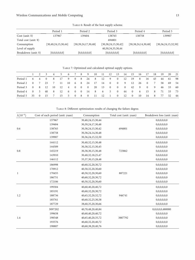
Table 6: Result of the best supply scheme.

Period 1 Period 2 Period 3 Period 4 Period 5

Cost (unit: ¥) 137967 139404 138765 138758 139907

Total cost (unit: ¥) 694801

Consumption [30,40,24,15,30,44] [30,39,24,17,30,48] [30,38,24,15,30,42] [30,38,24,14,30,48] [30,36,24,15,32,50]

Level of supply 40,50,34,35,30,44

Breakdown (unit: ¥) [0,0,0,0,0,0] [0,0,0,0,0,0] [0,0,0,0,0,0] [0,0,0,0,0,0] [0,0,0,0,0,0]

Table 7: Optimized and calculated optimal supply options.

1 2 3 4 5 6 7 8 9 10 11 12 13 14 15 16 17 18 19 20 21

Period 1 6 4 0 8 17 9 0 8 24 8 12 9 0 12 19 8 16 43 44 61 98

Period 2 0 7 23 7 11 10 6 8 24 17 14 0 0 9 12 26 0 7 58 69 54

Period 3 0 8 12 10 12 4 0 0 0 20 13 0 0 0 42 9 0 9 46 33 60

Period 4 0 5 40 8 12 6 0 0 14 8 6 5 0 44 0 6 15 8 71 33 73

Period 5 35 0 15 7 15 5 0 8 0 11 12 1 0 12 0 10 14 8 77 32 44

Table 8: Different optimization results of changing the failure degree.

λ 10−4

Cost of each period (unit: yuan) Consumption Total cost (unit: yuan) Breakdown loss (unit: yuan)

0.6

137967 30,40,24,15,30,44

694801

0,0,0,0,0,0

139404 30,39,24,17,30,48 0,0,0,0,0,0

138765 30,38,24,15,30,42 0,0,0,0,0,0

138758 30,38,24,14,30,48 0,0,0,0,0,0

139907 30,36,24,15,32,50 0,0,0,0,0,0

0.8

144112 30,40,32,15,30,48

723862

0,0,0,0,0,0

144509 30,38,32,15,30,45 0,0,0,0,0,0

145219 30,38,30,15,30,48 0,0,0,0,0,0

143910 30,40,32,18,25,47 0,0,0,0,0,0

146112 35,37,30,15,28,48 0,0,0,0,0,0

1

186998 40,60,32,20,30,72

887221

0,0,0,0,0,0

170912 40,50,32,20,30,60 0,0,0,0,0,0

170455 40,50,32,20,30,60 0,0,0,0,0,0

186751 40,60,32,20,30,72 0,0,0,0,0,0

172106 40,50,32,20,30,60 0,0,0,0,0,0

1.2

199304 40,60,40,20,40,72

946741

0,0,0,0,0,0

185191 40,60,32,20,30,72 0,0,0,0,0,0

188756 40,65,32,20,32,72 0,0,0,0,0,0

185761 40,60,32,25,30,58 0,0,0,0,0,0

187729 38,60,35,20,30,66 0,0,0,0,0,0

1.4

3097202 40,70,48,20,40,84

3887792

0,0,0,0,0,480000

199658 40,60,40,20,40,72 0,0,0,0,0,0

198548 40,65,40,20,35,72 0,0,0,0,0,0

193576 40,60,32,20,40,72 0,0,0,0,0,0

198807 40,60,38,20,40,76 0,0,0,0,0,0


first-echelon supply center to the second-echelon reloadingpoint 1; column 20 is the sum of columns 7-12, that is, thetransfer volume of the transfer of the first-echelon supplycenter to the second-echelon reloading point 2; column 21is the sum of 13-18, that is, the transfer volume of thefirst-echelon supply center to the second-echelon reloadingpoint 3.

6. Result Analysis

6.1. Different Failure Degree (λ) Analysis. As shown inTable 8, change the size and observe the different optimiza-tion results of the model and algorithm.

As can be seen from Table 8, with the increasing failuredegree (λ), the consumption of the whole process is gradu-ally increasing and the demand for spare parts is increasing.As a result, the preset inventory node is difficult to meet theconsumption of spare parts during the process of supply.

When λ reached 1:4 × 10−4, there is a delayed loss, and inthe actual supply of spare parts, delay consumption shouldbe eliminated or avoided as far as possible.

6.2. Different Quantity of Inventory to Supply Analysis. Ascan be seen from Table 9, when the inventory node isreduced, the consumption of spare parts is increasing con-tinuously, the same as the failure degree, and the cost of eachperiod is also increased. On the other hand, the reduction ofthe inventory node leads to insufficient advance supply time.Eventually, there is a breakdown loss when the inventorynode drops to 20,20,10,25,10,8.

6.3. Compared with Results of Traditional ðs, SÞ Policy. Inorder to test the effect of the model and algorithm optimiza-tion, the model is compared with the traditional ðs, SÞ policybased on different inventory nodes.

Table 9: Different optimization results of quantity of inventory to supply.

No.Quantity of inventory to

supplyCost of each period (unit:

yuan)Consumption

Total cost (unit:yuan)

Breakdown loss (unit:yuan)

1

608050455080

137967139404138765138758139907

30,40,24,15,30,4430,39,24,17,30,4830,38,24,15,30,4230,38,24,14,30,4830,36,24,15,32,50

694801

0,0,0,0,0,00,0,0,0,0,00,0,0,0,0,00,0,0,0,0,00,0,0,0,0,0

2

304026303032

170619144536144443145630144931

40,50,32,20,30,6030,40,32,15,30,4830,40,32,17,30,4630,35,32,20,30,5030,37,32,23,30,48

750160

0,0,0,0,0,00,0,0,0,0,00,0,0,0,0,00,0,0,0,0,00,0,0,0,0,0

3

304018302032

183044178905170547177920178959

40,50,40,20,40,6040,50,32,20,40,6040,50,32,20,30,6040,50,32,20,40,6040,55,32,28,30,72

889374

0,0,0,0,0,00,0,0,0,0,00,0,0,0,0,00,0,0,0,0,00,0,0,0,0,0

4

203018252020

209023199406198954199432200665

50,60,40,25,40,7240,60,40,20,40,7240,65,40,35,40,7240,60,44,38,35,7240,60,40,20,40,64

1007481

0,0,0,0,0,00,0,0,0,0,00,0,0,0,0,00,0,0,0,0,00,0,0,0,0,0

5

203010252020

215198210139209519209863209379

50,60,48,25,40,7250,60,40,25,40,7250,65,40,32,40,7250,60,40,25,40,7050,55,40,30,40,72

1054098

0,0,0,0,0,00,0,0,0,0,00,0,0,0,0,00,0,0,0,0,00,0,0,0,0,0

6

20201025108

31127423114210311059531142973111409

50,70,48,25,50,8450,70,48,25,60,7850,70,60,25,50,8050,70,50,25,50,8250,80,48,25,50,84

15563254

0,0,0,0,0,4800000,0,0,0,1000000,00,0,1600000,0,0,00,0,0,0,0,240000

0,2500000,0,0,0,480000


Table 10 is the model optimization comparison resultsbased on the inventory node sk = ½60,80,50,45,50,80�. It canbe seen from the table that the consumption of the adjustmentmodel is lower so that the cost of the traditional model is lowerthan that of the improved model in this paper. However, fromthe comparison optimized results based on the inventory nodesk = ½20,20,10,25,10,8� in Table 9, the consumption of theadjustmentmodel proposed in this paper is lower. At the sametime, when the inventory node is in this state, the traditionalmodel cannot meet the consumption in the supply periodbecause the consumption of spare parts is not considered. Thisleads to delays and breakdown loss.

Although the cost of the traditional model is lower thanthat of this paper when setting lower supply nodes, considering

the fault tolerance and stability of the whole model, the modelproposed in this paper canmeet the lower demand of inventorynodes while ensuring the stable supply of spare parts. It is inorder to ensure that there are no delays and delay losses asmuch as possible and make it more stable and reliable.

6.4. Comparison between Improved Algorithm and TraditionalAlgorithm. In order to analyze the effect of the improved algo-rithm, the joint model is also calculated by the traditional PSOalgorithm. The comparison result is shown in Table 11.

From Table 11, it is very obvious that the results of thefirst and second calculation through the traditional algo-rithm are in the position of local optimization. The systemcalculates the final result only once. Even the third result is

Table 10: Comparison of No. 6 supply node with the traditional ðs, SÞ policy.Cost of each period (unit: yuan) Consumption Total cost (unit: yuan) Breakdown loss (unit: yuan)

Traditional model

3078278 50,70,48,25,50,84

15395954

0,0,0,0,0,480000

3078580 50,70,60,25,60,82 0,0,160000,0,100000,240000

3079982 55,70,52,30,50,82 0,0,320000,0,0,240000

3079691 50,76,48,40,53,80 0,0,0,0,300000,0

3079422 50,70,48,25,48,84 0,0,0,0,0,480000

Improved model

199304 40,60,40,20,40,72

946741

0,0,0,0,0,0

185191 40,60,32,20,30,72 0,0,0,0,0,0

188756 40,65,32,20,32,72 0,0,0,0,0,0

185761 40,60,32,25,30,58 0,0,0,0,0,0

187729 38,60,35,20,30,66 0,0,0,0,0,0

Table 11: Comparison between the improved algorithm and the traditional algorithm.

Cost of each period (unit: yuan) Consumption Total cost (unit: yuan) Breakdown loss (unit: yuan)

Improved algorithm

137967 30,40,24,15,30,44

694801

0,0,0,0,0,0

139404 30,39,24,17,30,48 0,0,0,0,0,0

138765 30,38,24,15,30,42 0,0,0,0,0,0

138758 30,38,24,14,30,48 0,0,0,0,0,0

139907 30,36,24,15,32,50 0,0,0,0,0,0

Traditional algorithm

1

288765 70,40,24,15,30,35

982756

150000,0,0,0,0,0

279907 30,38,24,15,64,58 0,0,0,0,140000,0

138569 30,37,24,15,30,42 0,0,0,0,0,0

137659 30,38,25,14,50,48 0,0,0,0,0,0

137856 30,36,24,15,32,40 0,0,0,0,0,0

2

186998 40,50,40,20,40,60

867222

0,0,0,0,0,0

160912 30,50,32,20,40,60 0,0,0,0,0,0

160455 30,50,32,20,30,60 0,0,0,0,0,0

186751 40,50,32,20,40,60 0,0,0,0,0,0

172106 40,55,32,28,30,72 0,0,0,0,0,0

3

139967 30,37,26,17,30,46

696718

0,0,0,0,0,0

139204 30,36,24,15,30,50 0,0,0,0,0,0

138765 30,38,24,15,30,42 0,0,0,0,0,0

139258 30,38,24,15,31,48 0,0,0,0,0,0

139524 32,39,24,17,30,48 0,0,0,0,0,0


higher than the result of improved algorithm. However, withthe effect of algorithm error, the final results of them can beseen as the same.

7. Conclusion

In this paper, the joint policy combines the inventory policy andspare part supply network. In the joint model, the multiperiodand multiechelon supply network is built, and the ðs, SÞ policyis improved by the random lead time and different customers’maximum inventory. Due to the nonlinear, nonmonotonic,and multiperiodic changes of the established model, animproved PSO algorithm is proposed. The algorithm used inthis paper is optimized by adding adaptive inertia weight andpenalty function to speed up the optimization efficiency andimprove the convergence effect. A case is given. The optionalsupply scheme is obtained by the proposed algorithm. Thesensitivity analysis is used to discuss the influence of importantparameters on the model cost. The statistical characteristics ofthe model are summarized to provide a reference for the nextintelligent decision. Except that, the comparison results con-cluding the traditional ðs, SÞ model and the traditional PSOalgorithm are analyzed. We hope that the joint policy and usedmethod can provide a reference for the spare part supply inindustry and military.

In this paper, the parameters in the inventory policy aregiven as known, which can regard as optimized objects inthe future research. In addition, it can continue to studythe supply of multikind spare parts under different lifetimedistribution and so on.

Data Availability

The data used to support the findings of this study areincluded within the article.

Conflicts of Interest

The authors declare that they have no conflicts of interest.

References

[1] C. C. Sherbrooke, “VARI-METRIC: improved approximationsfor multi-indenture, multi-echelon availability models,” Oper-ations Research, vol. 34, no. 2, pp. 311–319, 1986.

[2] Q. Hu, S. Chakhar, S. Siraj, and A. Labib, “Spare parts classifi-cation in industrial manufacturing using the dominance-based rough set approach,” European Journal of OperationalResearch., vol. 262, no. 3, pp. 1136–1163, 2017.

[3] A. A. Ghobbar and C. H. Friend, “Evaluation of forecastingmethods for intermittent parts demand in the field of aviation:a predictive model,” Computers & Operations Research.,vol. 30, no. 14, pp. 2097–2114, 2003.

[4] R. Min, Q. Chen, and Z. Shen, Spare Parts Supply Science,National Defense Industry Press, 2013.

[5] R. P. Covert and G. C. Philip, “An EOQ model for items withWeibull distribution deterioration,” A I I E Transactions.,vol. 5, no. 4, pp. 323–326, 1973.

[6] S. Bashyam and M. C. Fu, “Optimization of (s, S) inventorysystems with random lead times and a service level constraint,”

Management Science., vol. 44, no. 12-part-2, pp. S243–S256,1998.

[7] S. Osaki, “An ordering policy with lead time,” InternationalJournal of Systems Science., vol. 8, no. 10, pp. 1091–1095, 1977.

[8] M. Issa, A. E. Hassanien, D. Oliva, A. Helmi, I. Ziedan, andA. Alzohairy, “ASCA-PSO: adaptive sine cosine optimizationalgorithm integrated with particle swarm for pairwise localsequence alignment,” Expert Systems with Applications,vol. 99, pp. 56–70, 2018.

[9] C. C. Sherbrooke, “Metric: a multi-echelon technique forrecoverable item control,” Operations Research, vol. 16, no. 1,pp. 122–141, 1968.

[10] T. S. Vaughan, “Failure replacement and preventive mainte-nance spare parts ordering policy,” European Journal of Oper-ational Research., vol. 161, no. 1, pp. 183–190, 2005.

[11] G. P. Cachon, “Exact evaluation of batch-ordering inventorypolicies in two-echelon supply chains with periodic review,”Operations Research, vol. 49, no. 1, pp. 79–98, 2001.

[12] W. J. Kennedy, J. Wayne Patterson, and L. D. Fredendall, “Anoverview of recent literature on spare parts inventories,” Inter-national Journal of Production Economics., vol. 76, no. 2,pp. 201–215, 2002.

[13] U. S. Rao, “Properties of the periodic review (R, T) inventorycontrol policy for stationary, stochastic demand,” M&SOM.,vol. 5, no. 1, pp. 37–53, 2003.

[14] Y. Wang and Q. Shi, “Improved dynamic PSO-based algo-rithm for critical spare parts supply optimization under (T,S) inventory policy,” IEEE Access., vol. 7, pp. 153694–153709,2019.

[15] M. C. Reade, A. Delaney, M. J. Bailey et al., “Prospective meta-analysis using individual patient data in intensive care medi-cine,” Intensive Care Medicine, vol. 36, no. 1, pp. 11–21, 2010.

[16] L. Spanjers, J. C. W. van Ommeren, and W. H. M. Zijm,“Closed loop two-echelon repairable item systems,” OR Spec-trum, vol. 27, no. 2-3, pp. 369–398, 2005.

[17] B.-T. Aharon, G. Boaz, and S. Shimrit, “Robust multi-echelonmulti-period inventory control,” European Journal of Opera-tional Research., vol. 199, no. 3, pp. 922–935, 2009.

[18] P. K. Aggarwal and K. Moinzadeh, “Order expedition in multi-echelon production/distribution systems,” IIE Transactions.,vol. 26, no. 2, pp. 86–96, 1994.

[19] A. Federgruen and P. Zipkin, “A combined vehicle routing andinventory allocation problem,” Operations Research, vol. 32,no. 5, pp. 1019–1037, 1984.

[20] J. Shu, C.-P. Teo, and Z.-J. M. Shen, “Stochastictransportation-inventory network design problem,” Opera-tions Research, vol. 53, no. 1, pp. 48–60, 2005.

[21] A. K. Saha, A. Paul, A. Azeem, and S. K. Paul, “Mitigatingpartial-disruption risk: a joint facility location and inventorymodel considering customers’ preferences and the role of sub-stitute products and backorder offers,” Computers & Opera-tions Research., vol. 117, p. 104884, 2020.

[22] S. Ekinci, D. Izci, and B. Hekimoğlu, “Optimal FOPID speedcontrol of DC motor via opposition-based hybrid Manta rayforaging optimization and simulated annealing algorithm,”Arabian Journal for Science and Engineering, vol. 46, no. 2,pp. 1395–1409, 2021.

[23] J. F. Farfán and L. Cea, “Coupling artificial neural networkswith the artificial bee colony algorithm for global calibrationof hydrological models,” Neural Computing and Applications,vol. 33, no. 14, pp. 8479–8494, 2021.


[24] A. S Sakthivel, A. D Mary, R. Vetrivel, and V. S. Kannan,“Optimal location of SVC for voltage stability enhancementunder contingency condition through PSO algorithm,” Inter-national Journal of Computer Applications, vol. 20, no. 1,pp. 30–36, 2011.

[25] M. Clerc and J. Kennedy, “The particle swarm - explosion, sta-bility, and convergence in a multidimensional complex space,”IEEE Trans. Evol. Computat., vol. 6, no. 1, pp. 58–73, 2002.

[26] Wen-Fung Leong and G. G. Yen, “PSO-based multiobjectiveoptimization with dynamic population size and adaptive localarchives,” IEEE Transactions on Systems, Man, and Cybernet-ics, Part B (Cybernetics), vol. 38, no. 5, pp. 1270–1293, 2008.

[27] E. Mezura-Montes and C. A. Coello Coello, “An improveddiversity mechanism for solving constrained optimizationproblems using a multimembered evolution strategy,” inGenetic and Evolutionary Computation–GECCO 2004, K.Deb, Ed., pp. 700–712, Springer, Berlin Heidelberg, Berlin,Heidelberg, 2004.

[28] Q. Hu, J. E. Boylan, H. Chen, and A. Labib, “OR in spare partsmanagement: a review,” European Journal of OperationalResearch., vol. 266, no. 2, pp. 395–414, 2018.

[29] M. Z. Ruan, Q. M. Li, Y. W. Peng, E. S. Ge, and A. L. Huang,“Model of spare part fill rate for systems of various structuresand optimization method,” Systems Engineering and Electron-ics., vol. 33, pp. 1799–1803, 2011.

[30] A. Mahor and S. Rangnekar, “Short term generation schedul-ing of cascaded hydro electric system using novel self adaptiveinertia weight PSO,” International Journal of Electrical Power& Energy Systems., vol. 34, no. 1, pp. 1–9, 2012.

[31] J. Kennedy and R. Eberhart, “Particle swarm optimization,” inProceedings of ICNN’95- International Conference on NeuralNetworks, IEEE, pp. 1942–1948, Perth, WA, Australia, 1995.

[32] K. Deep, “Madhuri: application of globally adaptive inertiaweight PSO to Lennard-Jones problem,” Proceedings of theInternational Conference on Soft Computing for Problem Solv-ing (Soc ProS 2011) December 20-22, 2011, K. Deep, A. Nagar,M. Pant, and J. C. Bansal, Eds., , pp. 31–38, Springer India,India, 2012.

[33] H. Shao and G. Zheng, “Boundedness and convergence ofonline gradient method with penalty and momentum,”Neuro-computing, vol. 74, no. 5, pp. 765–770, 2011.

[34] P. Sincak, “Intelligent technologies-theory and applications:new trends in intelligent technologies,” IOS Press, Ohmsha,Amsterdam; Washington, DC: Tokyo, 2002.

[35] A. C. Nearchou, “The effect of various operators on the geneticsearch for large scheduling problems,” International Journal ofProduction Economics., vol. 88, no. 2, pp. 191–203, 2004.


a joint optimization model of ðs inventory and supply

Documents