A Jacobian-free Edged-based Galerkin Formulation for Compressible Flows

Song Gao1, Wagdi G. Habashi2 CFD Laboratory McGill University, Montreal, QC, H3A 2S6, Canada

Dario Isola3 and Guido S. Baruzzi4 ANSYS, Inc., Montreal, QC, H3A 2M7, Canada

Marco Fossati5 University of Strathclyde, Glasgow, G1 1XJ, UK

A parallel formulation of a Jacobian-free all Mach numbers solver on unstructured

hybrid meshes is proposed. The Finite Element formulation is edge-based with flow

stabilization obtained with either AUSM+-up or Roe scheme. The linear system is solved via

a Jacobian-Free Newton-Krylov (JFNK) method with Lower-Upper Symmetric Gauss-

Seidel (LU-SGS) used as matrix-free preconditioner. The traditional formulation of LU-SGS

is enriched by including the contributions from viscous fluxes and boundary conditions. The

accuracy and efficiency of the proposed approach are demonstrated over cases ranging from

low to high Mach numbers: subsonic flow over the Trap Wing, transonic flow over the

ONERA M6 wing, supersonic flow over a sphere, supersonic flow over a waverider and

finally hypersonic flow over a sphere.

I. Introduction

he adoption of a unified approach for the numerical study of aircraft aerodynamics over a wide range of Mach

numbers is at the basis of the design of next-generation high-performance civil transport aircraft. In order to meet

demands in terms of reduced fuel consumptions, sustainability and safety, it is necessary to maintain high aero-

1 Doctoral candidate, CFD Laboratory, Department of Mechanical Engineering, 688 Sherbrooke Street West, AIAA Member. 2 Professor and Director, CFD Laboratory, Department of Mechanical Engineering, 688 Sherbrooke Street West, AIAA Fellow. 3 Senior Software Developer, ANSYS, Inc., 680 Sherbrooke Street West, AIAA Member. 4 Technical Fellow, ANSYS, Inc., 680 Sherbrooke Street West, AIAA Member. 5 Lecturer, Department of Mechanical and Aerospace Engineering, 75 Montrose Street, AIAA Member.

T

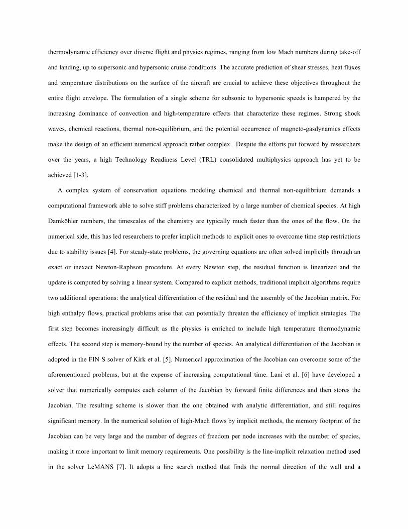
thermodynamic efficiency over diverse flight and physics regimes, ranging from low Mach numbers during take-off

and landing, up to supersonic and hypersonic cruise conditions. The accurate prediction of shear stresses, heat fluxes

and temperature distributions on the surface of the aircraft are crucial to achieve these objectives throughout the

entire flight envelope. The formulation of a single scheme for subsonic to hypersonic speeds is hampered by the

increasing dominance of convection and high-temperature effects that characterize these regimes. Strong shock

waves, chemical reactions, thermal non-equilibrium, and the potential occurrence of magneto-gasdynamics effects

make the design of an efficient numerical approach rather complex. Despite the efforts put forward by researchers

over the years, a high Technology Readiness Level (TRL) consolidated multiphysics approach has yet to be

achieved [1-3].

A complex system of conservation equations modeling chemical and thermal non-equilibrium demands a

computational framework able to solve stiff problems characterized by a large number of chemical species. At high

Damköhler numbers, the timescales of the chemistry are typically much faster than the ones of the flow. On the

numerical side, this has led researchers to prefer implicit methods to explicit ones to overcome time step restrictions

due to stability issues [4]. For steady-state problems, the governing equations are often solved implicitly through an

exact or inexact Newton-Raphson procedure. At every Newton step, the residual function is linearized and the

update is computed by solving a linear system. Compared to explicit methods, traditional implicit algorithms require

two additional operations: the analytical differentiation of the residual and the assembly of the Jacobian matrix. For

high enthalpy flows, practical problems arise that can potentially threaten the efficiency of implicit strategies. The

first step becomes increasingly difficult as the physics is enriched to include high temperature thermodynamic

effects. The second step is memory-bound by the number of species. An analytical differentiation of the Jacobian is

adopted in the FIN-S solver of Kirk et al. [5]. Numerical approximation of the Jacobian can overcome some of the

aforementioned problems, but at the expense of increasing computational time. Lani et al. [6] have developed a

solver that numerically computes each column of the Jacobian by forward finite differences and then stores the

Jacobian. The resulting scheme is slower than the one obtained with analytic differentiation, and still requires

significant memory. In the numerical solution of high-Mach flows by implicit methods, the memory footprint of the

Jacobian can be very large and the number of degrees of freedom per node increases with the number of species,

making it more important to limit memory requirements. One possibility is the line-implicit relaxation method used

in the solver LeMANS [7]. It adopts a line search method that finds the normal direction of the wall and a

renumbering algorithm that reorders the elements, and then the off-tridiagonal terms of the linearized system are

moved to the right-hand-side, whereas the left-hand-side tridiagonal system is solved by a point-iterative method

without storing the Jacobian. In the Jacobian-Free Newton-Krylov (JFNK) method adopted in this work the

Jacobian-vector product is approximated by a Fréchet derivative, which circumvents the need to store the full

Jacobian, and a Krylov subspace method is used to solve the linear system [8].

The effectiveness of Krylov subspace linear system solvers depends on good preconditioners. The widely-used

Incomplete Lower-Upper (ILU) factorization not only requires storing the system matrix but also its factorization,

thus doubling the memory footprint. To the best of the authors’ knowledge, three alternate options are available. The

first one is the Jacobi preconditioner, which can be implemented in a Jacobian-free fashion. This method only

requires the diagonal of the Jacobian. While it seems numerically advantageous, a large number of linear iterations

might be required for convergence. The second alternative is the multiplicative-additive Schwarz preconditioned

inexact Newton [9] approach, which is a nonlinear Jacobian-free preconditioning method designed to overcome

unbalanced nonlinearities coming from different ranges of time and spatial scales, such as shock waves and reaction

fronts, but only two-dimensional incompressible flow test cases have been presented in the reference. The last

alternative, adopted in this work, is LU-SGS [4]. It was originally developed as a solver for inviscid flows on

structured grids, but has recently been extended to viscous flows and unstructured meshes [10] [11]. In LU-SGS, the

implicit operator is simplified by introducing a Roe-type flux approximation that replaces the Roe matrix with its

spectral radius, consequently only the diagonal part of the Jacobian is stored and the products of the off-diagonal

terms and the solution update are approximated by a Fréchet derivative through a forward and a backward sweep.

However, in the original LU-SGS, the viscous Jacobian is identified as a scalar in the spectral radius and the

contributions from boundary conditions are omitted. In this work, the viscous Jacobian is taken into account by

computing it on the fly during the two sweeps. Riemann, supersonic outlet, slip wall and non-slip wall boundary

conditions are included in the computation of the Jacobian.

This article is organized as follows: Section II will illustrate the governing equations, while Section III will

present the numerical formulation and Section IV will present some numerical results for validation. The test cases

for the present work are limited to non-reactive flows in thermal equilibrium. This is a necessary step to assess the

characteristics of the method before introducing the more complex non-equilibrium effects and the corresponding

numerical formulation.

II. Governing Equations

Let us recall for completeness the equations governing unsteady compressible viscous flows in conservative

form [12, 13]

( )A VQ (Q) ( ) 0QQ,t

∂∇+∇⋅ − =

∂F F (II.1)

where Q is the vector of conservative variables, i.e. Q=[ρ,ρV,ρet].ρV is the momentum vector and et is the total

energy per unit mass and it is defined as the sum of the internal and kinetic energy. FA and FV are the inviscid and

viscous fluxes, respectively. The inviscid fluxes in Cartesian coordinates are

ρ⎧ ⎫⎪ ⎪ρ +⎪ ⎪⎪ ⎪

= ρ⎨ ⎬⎪ ⎪ρ⎪ ⎪

ρ +⎪ ⎪⎩ ⎭t

2

Ax

uu P

F uvuw

u( e P)

;

ρ⎧ ⎫⎪ ⎪ρ⎪ ⎪⎪ ⎪

= ρ +⎨ ⎬⎪ ⎪ρ⎪ ⎪

ρ +⎪ ⎪⎩ ⎭t

A 2y

vuv

F v Pvw

v( e P)

;

ρ⎧ ⎫⎪ ⎪ρ⎪ ⎪⎪ ⎪

= ρ⎨ ⎬⎪ ⎪ρ +⎪ ⎪

ρ +⎪ ⎪⎩ ⎭t

Az

2

wuw

F vww P

w( e P)

(II.2)

The viscous fluxes in Cartesian coordinates are

⎧ ⎫⎪ ⎪τ⎪ ⎪⎪ ⎪

= τ⎨ ⎬⎪ ⎪τ⎪ ⎪τ⎪ ⎪⎩ ⎭

xxVx xy

xz

x

0

F

V

;

⎧ ⎫⎪ ⎪τ⎪ ⎪⎪ ⎪τ= ⎨ ⎬⎪ ⎪τ⎪ ⎪τ⎪ ⎪⎩ ⎭

yxV

yyy

yz

y

0

F

V

;

⎧ ⎫⎪ ⎪τ⎪ ⎪⎪ ⎪

= τ⎨ ⎬⎪ ⎪τ⎪ ⎪τ⎪ ⎪⎩ ⎭

zxVz zy

zz

z

0

F

V

(II.3)

Newton’s law for the stress tensor and the Stokes hypothesis are adopted and a calorically perfect ideal gas is

assumed.

III. Numerical Methods

A. Edge-based Stable Finite Element Discretization

A Finite Element edge-based assembly [14] is adopted to allow the application of either AUSM+up [15] or Roe

[16] scheme to stabilize the advection terms. The edge-based assembly easily handles hybrid meshes with a unique

data structure [17] and it is computationally more efficient than the traditional element-based one [18]. For steady-

state flows, the weak-Galerkin formulation of Eq. (II.1) is adopted:

( )∈ ∈

⋅∇ − + − =∑ ∑∫ ∫i i

i ie

A V A V

e E e FV A

W ( ) V W· dA 0dF F n F F (III.1)

where Wi is the i-th linear Lagrangian test function, Ei and Fi are the set of elements/boundary faces sharing the i-th

vertex. For ease of notation, the contribution from boundary conditions will be ignored from this point on. The first

term of the above equation can be assembled in an edge-based fashion as [19]:

i i ei

A A A Aj i j i

iE

Vij ij

j K j K e V

dW V 02 2 ∈∈ ∈

+ −− + ∇∑ ∑ ∑ ∫·

F F F·

FF·η χ = (III.2)

where Ki is the set of nodes connected to the i-th node via an edge. The edge coefficients are defined as

∈ ∈

⎛ ⎞−⎜ ∇ ⎟∇

⎜ ⎟⎝ ⎠

= =∫ ∫∑ ∑∫e ei i

ji iV V

j ie E e E A

ij ij jd d aW W W V nV W d dAWWnη χ (III.3)

where the coefficient χij is defined only for boundary edges. Another second order edge coefficient tensor dij can be

defined as

i e

ij ij ij ijsT T

ij i je E

aij ij

V

d d d dd W d d , d

2 2( ) ( )

W V ,∈

+ −= = =∇ ∇∑∫ (III.4)

To provide stabilization for advection-dominated flows, the vector of inviscid fluxes FA is replaced with a

numerical counterpart,Φnum evaluated at the edge’s midpoint, i.e.

i i ei

A Aj inum V

ij ijj K

ij V

ie

jEK

,(Q Q , W) V 02

d∈∈ ∈

−Φ − ⋅ + ∇ ⋅ =∑ ∑ ∑∫

F FFη χ (III.5)

The numerical inviscid fluxes for Φnum can be either AUSM+-up or Roe fluxes, nonlinear functions of the nodal

variables and of the edge coefficients. The boundary-edge term of Eq. (III.5) can be seen as a “correction” factor,

since it is proportional to the difference of fluxes along the edge. Following [14], it is left untouched and no

additional dissipation is introduced for boundary edges. The numerical scheme is made second-order by adopting a

MUSCL [20] reconstruction of the primitive variables at the edges’ midpoint and standard 1D slope limiters [21,

22]. The viscous fluxes are discretized with the continuous Galerkin approximation and assembled in an edge-based

fashion, naturally resulting in a second-order representation [14].

B. Jacobian-free Newton-Krylov Solver

The JFNK [8] strategy is introduced by making use of a pseudo-transient continuation method where the original

steady problem is transformed into a pseudo-unsteady one [23], i.e.

n n 1

n nn

Q Qr R(Q ) 0, n 1,2,...−−

= + = =Δτ

L (III.6)

where L is the lumped mass matrix, R is the left-hand-side of Eq. (III.5). The pseudo-time step Δτn is chosen to

locally satisfy the CFL stability condition for linear advection problems and is in general increased as the solution

progresses. At each iteration of the Newton procedure, the solution update is computed as

n

nRI Q ( )R QQ∂⎡ ⎤+ Δ = −⎢ ⎥Δτ ∂⎣ ⎦

L (III.7)

Note that small values of Δτn increase the diagonal dominance of the system matrix, making it easier to invert.

As Δτn increases, the first term of Eq. (III.7) gradually vanishes and the pseudo-unsteady problem reverts to the

standard Newton’s method. The above linear system is solved by means of the Flexible Generalized Minimal

Residual method (FGMRES) [24]. FGMRES is an iterative solver for non-symmetric linear systems where the

preconditioner can vary at each iteration. The convergence of FGMRES depends on the condition number of the

matrix; preconditioning techniques can be enforced to cluster the eigenvalues of the matrix and to improve the

convergence of the linear system. Defining

L ∂⎡ ⎤= +⎢ ⎥Δτ ∂⎣ ⎦

n

AQRI and P M QΔ = Δ

and the preconditioner by M, the right preconditioning results

1)((AM P) R− Δ = − (III.8)

FGMRES only accesses the matrix through matrix-vector multiplications, therefore it is not necessary to form

and store the matrix A. In the framework of Jacobian-free methods, the product of the preconditioned system matrix

with the preconditioned solution is replaced by a Fréchet derivative, i.e.

1

n1

n

n1

1

(AM

R)( )

)( P)

(AM P M PQ

Q (Q M P (R Q) R )

− −

−−

Δ

∂⎡ ⎤Δ + Δ⎢ ⎥Δτ ∂⎣ ⎦

Δ ε Δ+

Δτ

−

ε

=

+; L

L

(III.9)

where ε is a suitably-chosen small number [25] defined as

n1 Q

error_relQ

+ε = ⋅

Δ (III.10)

with error_rel being the square root of the machine precision.

Note that the JFNK methods require one evaluation of the residual function Rat each FGMRES iteration, while

traditional methods that explicitly form the Jacobian require one matrix-vector product per FGMRES iteration. For a

problem of millions of unknowns, one evaluation of the residual function typically requires more time than one

matrix-vector multiplication, indicating that overall JFNK might be slower than traditional methods. It is also worth

mentioning that the JFNK methods only require the evaluation of R, but not its derivatives, which enables the

computation of the inviscid contribution to the Jacobian matrix through the MUSCL-reconstructed state with slope-

limiter, or a simple piecewise constant reconstruction of the solutions.

C. Lower-Upper Symmetric-Gauss-Seidel (LU-SGS) Preconditioner

In order to obtain a truly Jacobian-free method, the preconditioning step must also be Jacobian-free. LU-SGS is

an efficient iterative solver specifically designed for advection-dominated flows that does not require storing the

Jacobian. Following [4], LU-SGS is applied by solving

A nQ R(Q )Δ = − (III.11)

through a forward and backward sweep, namely

D LD U D

*

*

( ) Q R

( ) Q Q

+ Δ = −

+ Δ = Δ (III.12)

where A is the sum of the pseudo-time contribution and the Jacobian of the approximate residual function

RA I

t Q∂

= +Δ ∂

L (III.13)

and D, U and L are the diagonal, upper and lower parts of matrixA, respectively.

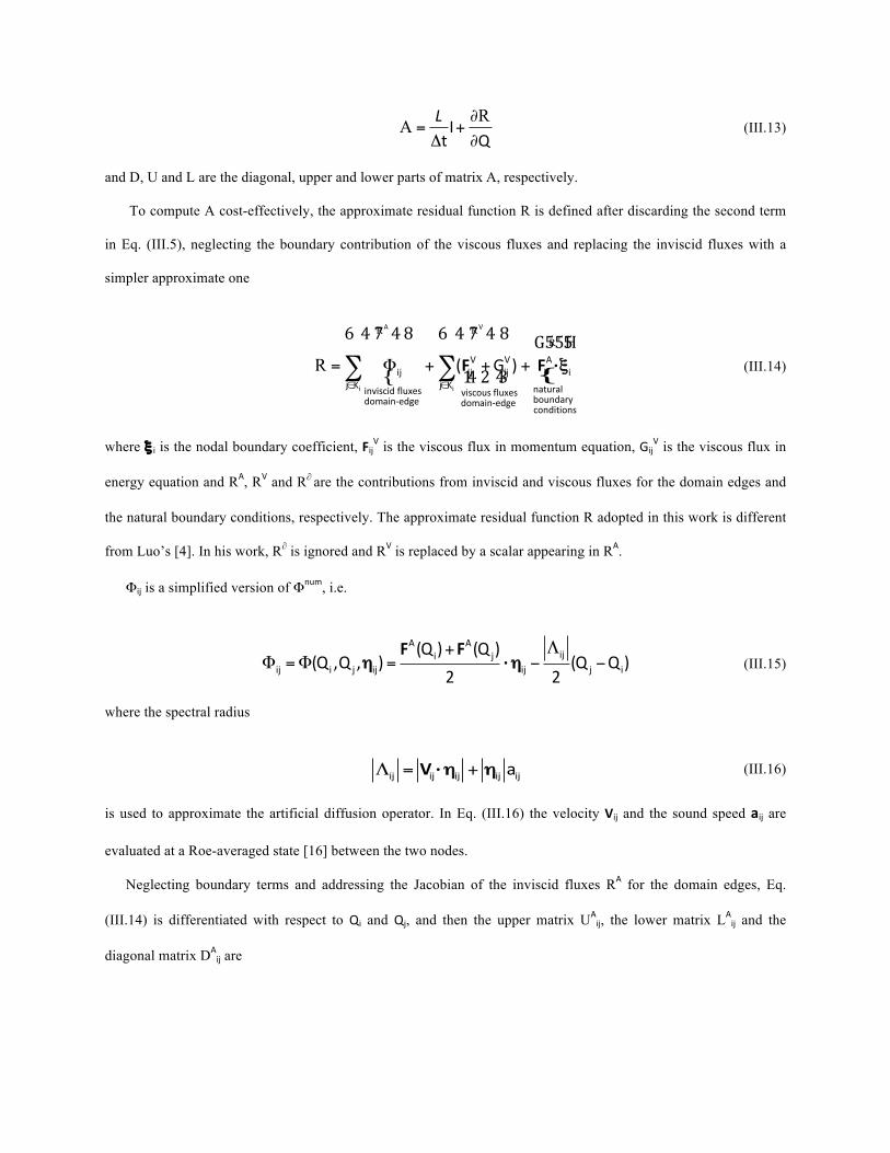
To compute A cost-effectively, the approximate residual function R is defined after discarding the second term

in Eq. (III.5), neglecting the boundary contribution of the viscous fluxes and replacing the inviscid fluxes with a

simpler approximate one

{ {

R RR

Ri i

A V

Aij i

naturalinviscid fluxes viscousfluxesboundarydomain-edge domain-edgecond

V Vij ij i

j

itions

K j K

( G )

∂

∈ ∈

= + + +Φ∑ ∑ ·F F

6 4 7 48 6 4 7 4 8 G555H

14 2 43 ξ (III.14)

where ξ i is the nodal boundary coefficient, FijV is the viscous flux in momentum equation, Gij

V is the viscous flux in

energy equation and RA, RV and R∂ are the contributions from inviscid and viscous fluxes for the domain edges and

the natural boundary conditions, respectively. The approximate residual function R adopted in this work is different

from Luo’s [4]. In his work, R∂ is ignored and RV is replaced by a scalar appearing in RA.

Φij is a simplified version of Φnum, i.e.

iji j

ij i j ij j

A

ij i

A (Q ) (Q )(Q ,Q , ) (Q Q )

2 2

Λ+= =Φ −Φ −

F F·η η (III.15)

where the spectral radius

ij ij ij ijij aΛ = +·V η η (III.16)

is used to approximate the artificial diffusion operator. In Eq. (III.16) the velocity Vij and the sound speed aij are

evaluated at a Roe-averaged state [16] between the two nodes.

Neglecting boundary terms and addressing the Jacobian of the inviscid fluxes RA for the domain edges, Eq.

(III.14) is differentiated with respect to Qi and Qj, and then the upper matrix UAij, the lower matrix LA

ij and the

diagonal matrix DAij are

U , L , DeA A N

ij ji ijj jij ij

j

A A A iij ij ii

j 1ij

1 12

I I ItQ 2 Q 2=

⎡ ⎤ ⎡ ⎤⋅ ⋅= − = − + = +⎢ ⎥ ⎢

⎡ ⎤Λ∂ ∂Λ Λ ⎢ ⎥

∂ ∂ ⎢ ⎥⎣ ⎦⎥

Δ⎢ ⎥ ⎢ ⎥⎣ ⎦ ⎣ ⎦∑

F F Lη η (III.17)

Note that the zero-sum property of the edge coefficients for domain nodes has been used and the pseudo-time

contribution has been added to the diagonal matrix. As a result, the 5x5 matrix located on the diagonal block is

replaced by a scalar, thus making its inversion a trivial operation.

With this strategy UA, LA and DA must be computed and explicitly stored, but this can be avoided by introducing

a Jacobian-free approximation of the matrix-vector product as

A

j *A * A

ij j j ij jj

j

j

i(Q Q ) (Q )Q

Q⋅ + εΔ −

=∂ ⋅ ⋅

Δ∂ ε

F F Fη η η (III.18)

where ε is defined in Eq. (III.10).

To address the Jacobian of RV, FijV and Gij

V are discretized with the standard continuous Galerkin approximation

and assembled in an edge-based fashion, as in [14]. The upper matrix UijV, the lower matrix Lij

V and the diagonal

matrix DijVare

D

D

U

L

V5,3

j i

5,1j i

j jVij 5,3 5,

V,s V,a V,s V,a iii ij ij ji ji

i j i

V,s V,a V,s V,a iij ij ij ij ji ji

i j i

V,s V,a V,s V,aij ij ij ij ij

Vii

1j j

Vij

I (A A ) (A A )

I (A A ) (A A

Q

)

I (A A ) I (A

Q

QA )

Q

<

<

<

<

= ⋅ − + − −

⋅

⎡ ⎤ ∂⎢ ⎥ ∂⎣ ⎦

⎡− + − ⋅ −

= ⋅ + ⋅ ⋅ +

⎤ ∂+ ⎢ ⎥ ∂⎣ ⎦

∂ ∂+

∂ ∂

=

∑ ∑

∑ ∑V V

V

V·

V V·V

j j5,3 5,1

j

V,s V,a V,s V,aji ji ij ji ji

j

I (A A ) IQ

(Q

A A )= ⋅ − ⋅∂ ∂

+∂

⋅ −∂

V VV ·

(III.19)

where the “s” and “a” superscripts indicate the symmetric and anti-symmetric part of a tensor, i.e.

V,s s V,a aij ij ij ij ij ij ij j i iji j= )I+( + ) , AA tr (d = - )(d dµ µ λ λ µ

(III.20)

The transformation matrices are

5,3

0 1 0 0 0I 0 0 1 0 0

0 0 0 1 0

T⎡ ⎤⎢ ⎥= ⎢ ⎥⎢ ⎥⎣ ⎦

and [ ]5,1I 0 0 0 0 1 T= (III.21)

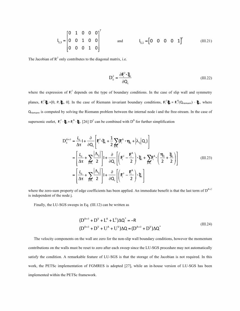
The Jacobian of R∂ only contributes to the diagonal matrix, i.e.

D∂

∂ ∂=

∂i

iii

iQF · ξ

(III.22)

where the expression of Fi∂ depends on the type of boundary conditions. In the case of slip wall and symmetry

planes, Fi∂·ξ i=[0, Piξ i, 0]. In the case of Riemann invariant boundary conditions, Fi∂·ξ i=FiA(Qriemann) · ξ i, where

Qriemann is computed by solving the Riemann problem between the internal node iand the free-stream. In the case of

supersonic outlet, Fi∂ ·ξ i=FiA·ξ i. [26] D∂ can be combined with DA for further simplification

D

D

Di

i i

i

A Aii i i ij i

i

Aij Ai

i ii

Aij i

i

iii ij

j K

ijii ii

j K j K

Aii

Aii

iii

j K i

I ( Q1 )Q

I2 Q 2 2 2

I2 Q

2

2

∈

∈

+

+∂ ∂

∂

∂

∈

∂

+∂

∈

⎡ ⎤+⎢ ⎥

⎣ ⎦

Λ ⎛

∂= + + λΔτ ∂

⎡ ⎤ ⎡ ⎤⎛ ⎞∂= + + − +⎢ ⎥ ⎢ ⎥⎜ ⎟Δτ ∂⎢ ⎥ ⎝ ⎠⎣ ⎦⎣ ⎦

⎡ ⎤ ⎡ ⎤∂= + + −⎢ ⎥ ⎢ ⎥

Δ

⎞+⎜ ⎟

⎝ ⎠

Λ ⎛ ⎞⎜ ⎟⎝ ⎠τ ∂⎢ ⎥ ⎣ ⎦⎣ ⎦

∑

∑ ∑

∑

F F

FF F

FF

· ·

· ·

·

L

L

L

ξ η

η ξξ

ξ

(III.23)

where the zero-sum property of edge coefficients has been applied. An immediate benefit is that the last term of DA+∂ is independent of the node j.

Finally, the LU-SGS sweeps in Eq. (III.12) can be written as

D D L LD D U U D D

+∂

+∂ +∂

+ + + Δ = −

+ + + Δ = + Δ

A V A V *

A V A V A V *

( ) Q R

( ) Q ( ) Q (III.24)

The velocity components on the wall are zero for the non-slip wall boundary conditions, however the momentum

contributions on the walls must be reset to zero after each sweep since the LU-SGS procedure may not automatically

satisfy the condition. A remarkable feature of LU-SGS is that the storage of the Jacobian is not required. In this

work, the PETSc implementation of FGMRES is adopted [27], while an in-house version of LU-SGS has been

implemented within the PETSc framework.

IV. Numerical Results

The proposed numerical method has been validated over a representative range of Mach numbers, for 3D test

cases. These are the subsonic flow over the Trap Wing, the transonic flow over the ONERA M6 wing, the Mach

1.93 laminar flow over a sphere, the Mach 4.0 turbulence flow over a waverider and the hypersonic flow over a

sphere.

With the present JFNK implementation the inviscid contribution to the Jacobian matrix can be computed either

using a simple piecewise-constant reconstruction of the solution, or a MUSCL reconstructed state with slope-limiter.

The first one will be subsequently referred to as 1st order Jacobian (JFNK-1), and the second as 2nd order Jacobian

(JFNK-2). In order to assess the performance of the JFNK solvers, the traditional method of explicitly forming the

Jacobian and using block-Jacobi with ILU preconditioning is also tested. This will subsequently be referred to as the

explicit Jacobian method. The explicit Jacobian method uses a simple piecewise-constant reconstruction of the

solution to compute the Jacobian. Computing the explicit Jacobian using the MUSCL reconstructed states and the

slope-limiter is difficult because a larger stencil is required to compute their derivatives. However, JFNK does not

have such a problem because its Jacobian is numerically approximated and the derivatives are not needed.

Unless otherwise specified, all the results shown in the following sections are obtained with JFNK-2. FGMRES

convergence is achieved when the relative drop in the preconditioned residual norm is below the specified tolerance

of10-4. The size of the Krylov space is 20. For the first three test cases, FGMRES is stopped when the number of

FGMRES iterations exceeds 20and the code proceeds to the next Newton step. No FGMRES restarts have been

allowed except for the last two test case. Stabilization is provided by the AUSM+-up or Roe scheme with the van

Albada slope limiter. The ILU preconditioner remains fixed at each FGMRES iteration, in which case the results of

FGMRES are identical to those of GMRES.

A. Mach 0.2 Viscous Flow past the Trap Wing

This example is the Mach 0.2 viscous flow around the Trap Wing from the First AIAA CFD High-Lift

Prediction Workshop [28]. The angle of attack is 13 degrees. The Reynolds number based on the mean

aerodynamic chord (MAC) is 4.3×106 and the turbulent flow is modeled with the Spalart-Allmaras turbulence

model, solved in a loosely coupled fashion. The computational grid, shown in Figure 1, consists of 8,188,411 nodes,

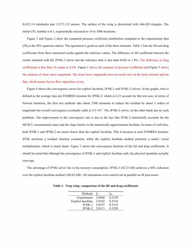
8,632,114 tetrahedra and 13,271,131 prisms. The surface of the wing is discretized with 446,420 triangles. The

initial CFL number is 0.1, exponentially increased to 10 in 1000 iterations.

Figure 1 and Figure 2 show the computed pressure coefficient distribution compared to the experimental data

[28] at the 50% spanwise station. The agreement is good on each of the three elements. Table 1 lists the lift and drag

coefficients from three numerical results against the reference values. The difference in lift coefficient between the

results obtained with the JFNK-2 solver and the reference data is less than 0.036 or 1.8%. The difference in drag

coefficients is less than 10 counts or 0.4%. Figure 1 shows the contours of pressure coefficient and Figure 3 shows

the contours of shear stress magnitude. The shear stress magnitude does not reach zero on the main element and the

flap, which means that no flow separation occurs.

Figure 4 shows the convergence curves for explicit Jacobian, JFNK-1 and JFNK-2 solvers. In the graphs, time is

defined as the average time per FGMRES iteration for JFNK-2, which is 6.15 seconds for this test case. In terms of

Newton iterations, the first two methods take about 1500 iterations to reduce the residual by about 3 orders of

magnitude but overall convergence eventually stalls at 2.5×10-7. The JFNK-2 solver, on the other hand, has no such

problems. The improvement in the convergence rate is due to the fact that JFNK-2 intrinsically accounts for the

MUSCL reconstructed states and the slope limiter in the numerically-approximated Jacobian. In terms of wall time,

both JFNK-1 and JFNK-2 are much slower than the explicit Jacobian. This is because at each FGMRES iteration,

JFNK performs a residual function evaluation, while the explicit Jacobian method performs a matrix vector

multiplication, which is much faster. Figure 5 shows the convergence histories of the lift and drag coefficients. It

should be noted that although the convergence of JFNK-1 and explicit Jacobian stall, the physical quantities actually

converge.

The advantage of JFNK solver lies in the memory consumption: JFNK-2 (42.22 GB) achieves a 60% reduction

over the explicit Jacobian method (106.62 GB). All simulations were carried out in parallel on 48 processors.

Table 1. Trap wing: comparison of the lift and drag coefficients

Methods CL CDExperiments 2.0468 0.3330

Explicit Jacobian 2.0102 0.3318 JFNK-1 2.0107 0.3319 JFNK-2 2.0113 0.3320

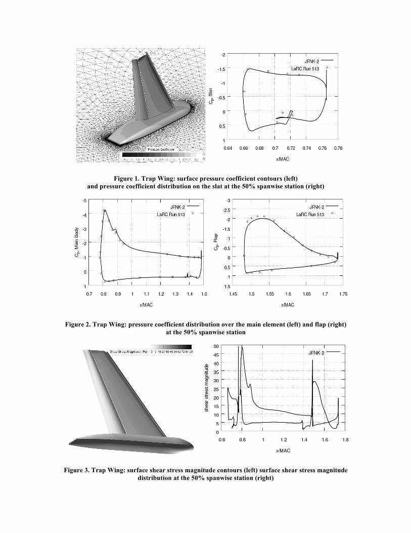
Figure 1. Trap Wing: surface pressure coefficient contours (left) and pressure coefficient distribution on the slat at the 50% spanwise station (right)

Figure 2. Trap Wing: pressure coefficient distribution over the main element (left) and flap (right) at the 50% spanwise station

Figure 3. Trap Wing: surface shear stress magnitude contours (left) surface shear stress magnitude distribution at the 50% spanwise station (right)

Figure 4. Trap Wing: convergence as a function of the number of iterations (left) and elapsed time (right)

Figure 5. Trap wing: convergence history of the lift (left) and drag coefficients (right)

Figure 6. ONERA M6 wing: final adapted mesh (left), Mach contours (right)

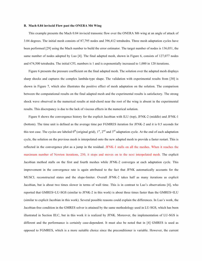
B. Mach 0.84 inviscid Flow past the ONERA M6 Wing

This example presents the Mach 0.84 inviscid transonic flow over the ONERA M6 wing at an angle of attack of

3.04 degrees. The initial mesh consists of 87,795 nodes and 396,412 tetrahedra. Three mesh adaptation cycles have

been performed [29] using the Mach number to build the error estimator. The target number of nodes is 136,051, the

same number of nodes adopted by Luo [4]. The final adapted mesh, shown in Figure 6, consists of 127,077 nodes

and 674,500 tetrahedra. The initial CFL numbers is 1 and is exponentially increased to 1,000 in 120 iterations.

Figure 6 presents the pressure coefficient on the final adapted mesh. The solution over the adapted mesh displays

sharp shocks and captures the complex lambda-type shape. The validation with experimental results from [30] is

shown in Figure 7, which also illustrates the positive effect of mesh adaptation on the solution. The comparison

between the computational results on the final adapted mesh and the experimental results is satisfactory. The strong

shock wave observed in the numerical results at mid-chord near the root of the wing is absent in the experimental

results. This discrepancy is due to the lack of viscous effects in the numerical solution.

Figure 8 shows the convergence history for the explicit Jacobian with ILU (top), JFNK-2 (middle) and JFNK-1

(bottom). The time unit is defined as the average time per FGMRES iteration for JFNK-2 and it is 0.5 seconds for

this test case. The cycles are labeled 0th (original grid), 1st, 2nd and 3rd adaptation cycle. At the end of each adaptation

cycle, the solution on the previous mesh is interpolated onto the new adapted mesh to provide a faster restart. This is

reflected in the convergence plot as a jump in the residual. JFNK-1 stalls on all the meshes. When it reaches the

maximum number of Newton iterations, 250, it stops and moves on to the next interpolated mesh. The explicit

Jacobian method stalls on the first and fourth meshes while JFNK-2 converges at each adaptation cycle. This

improvement in the convergence rate is again attributed to the fact that JFNK automatically accounts for the

MUSCL reconstructed states and the slope-limiter. Overall JFNK-2 takes half as many iterations as explicit

Jacobian, but is about two times slower in terms of wall time. This is in contrast to Luo’s observations [4], who

reported that GMRES+LU-SGS (similar to JFNK-2 in this work) is about three times faster than the GMRES+ILU

(similar to explicit Jacobian in this work). Several possible reasons could explain the differences. In Luo’s work, the

Jacobian-free condition in the GMRES solver is attained by the same methodology used in LU-SGS, which has been

illustrated in Section III.C, but in this work it is realized by JFNK. Moreover, the implementation of LU-SGS is

different and the performance is certainly case-dependent. It must also be noted that in [4] GMRES is used as

opposed to FGMRES, which is a more suitable choice since the preconditioner is variable. However, the current

performance result is similar to that of Qin [31] who showed that the matrix-free solver takes more CPU time than

explicit Jacobian.

Figure 7. ONERA M6 wing: comparison of the computed surface pressure coefficients on the initial and final adapted mesh with the experimental results at the 20%, 44%, 65%, 80%, 90% and 95% spanwise stations

Figure 8. ONERA M6 wing: comparison of the convergence history as a function of the number of iterations (left) and time (right) between the explicit Jacobian (top), JFNK-2 (middle) and JFNK-1 (bottom)

C. Mach 1.93 Viscous Flow past a Sphere

This example presents the Mach 1.93 viscous flow around a sphere. The sphere radius R is 7.5 mm, the

freestream temperature and pressure are 294 K and 540 Pa, respectively. The Reynolds number based on the sphere

radius is 1750, which is small enough to assume laminar flow. The computational grid, shown in Figure 9, consists

of 300,993 nodes, 281,484 tetrahedra and 487,680 prisms. The surface of the sphere is represented by 8,128

triangles. The near-wall region is represented by 60 layers of prisms and is approximately 3.9R thick. The initial

CFL value of 10-1 is exponentially increased to 100 in 500 iterations.

Figure 9. Mach 1.93 viscous flow over a sphere: hybrid grid (left) and Mach number contours (right)

Figure 10. Mach 1.93 viscous flow over a sphere: non-dimensional density along the line normal to the axis in front of the sphere (left) and along the line normal to the sphere (right)

The Mach contours are shown in Figure 9. A bow shock appears in front of the sphere. The non-dimensional

density is plotted in Figure 10 along the crosswind direction at two different locations: at the nose, x=R, and at the

mid-section, x=0. The crosswind coordinate is scaled with respect to the distance between the shock location, ys,

and the boundary location, yb. Since neither of the references provides a value for it, ys is measured from the

solution: ys(x=0)=2.743R and ys(x=R)=1.32R. The agreement between the solution obtained with the proposed

method and the results of Gnoffo [32] is fairly good, and so is the agreement with the experiments [32]. Both the

present computation and the result by Gnoffo under predict the value of the density at the stagnation point.

Figure 11. Mach 1.93 viscous flow over a sphere: convergence history as a function of the number of iterations (left) and time (right)

Figure 12. Mach 1.93 viscous flow over a sphere: convergence history of the LU-SGS and Jacobi preconditioners

Figure 13. Mach 1.93 viscous flow over a sphere: convergence history of the LU-SGS and Luo’s LU-SGS preconditioners as a function of the number of iterations (left) and time (right)

Figure 11 shows the convergence history for the explicit Jacobian, JFNK-1 and JFNK-2. Time is defined as the

average time per FGMRES iteration for JFNK-2, which is 0.48s for this test case. All the residuals converge to 10-10.

The advantage of JFNK-2 is in the number of Newton iterations, only 626. This is expected because JFNK-2

includes the MUSCL reconstructed states and the slope-limiter in the approximate Jacobian. In terms of wall time,

JFNK-1 and JFNK-2 take about the same time. Both of them are about 6 times slower than the explicit Jacobian

method. In terms of the maximum memory storage, JFNK-2 (1.48 GB) achieves a 54% reduction over explicit

Jacobian (3.18 GB). All simulations were run in parallel on 4 processors.

Figure 12 shows the comparison between JFNK-1 with LU-SGS and JFNK-1 with the Jacobi preconditioner.

In conjunction with the LU-SGS preconditioner, FGMRES convergence is achieved when the relative drop in

the preconditioned residual norm is below the specified tolerance of 10-2 or a maximum number of FGMRES

iterations 20, whereas for the Jacobi preconditioner the tolerance was set at 10-6 and the maximum number of

FGMRES iterations was set to 200. In general, Jacobi is a less effective preconditioner than LU-SGS and thus

requires more linear iterations to converge. The size of the Krylov space is 20 for both methods. Stabilization is

provided by the AUSM+-up scheme with the van Albada slope limiter. Although more FGMRES iterations are

allowed in the case of the Jacobi preconditioner, it still fails at around 500 Newton iteration. This suggests that the

Jacobi preconditioner is, for this case, less robust than LU-SGS. Note that the chosen maximum number of linear

iterations is ten times greater for Jacobi, but it is not sufficient to prevent numerical instabilities. Figure 13 shows the

comparison between JFNK-2 with LU-SGS and Luo’s LU-SGS preconditioner [4]. The maximum CFL is 100 for

LU-SGS and 1 for Luo’s LU-SGS. The cases of maximum CFLs 100 and 10 have been tested for Luo’s LU-SGS,

but both fail due to negative temperature, which suggests that robustness increases when the contributions from the

boundaries are included and more accurate viscous fluxes are adopted.

An analysis of the effects of the relative tolerance level and maximum number of FGMRES iterations

(ksp_max_it) was carried out. Two relative tolerance levels were considered,10-2 and 10-6. Themaximum number of

FGMRES iterations was set to 5, 10, 40, 80, 120, 160 and 200. Figure 14 displays the results obtained with a relative

tolerance of 10-2 and different values of maximum number of FGMRES iterations for the explicit Jacobian method

(top), JFNK-1 (middle) and JFNK-2 (bottom). The left column shows the convergence history in terms of Newton

iterations. The middle column shows the convergence history in terms of time units. The right column shows the

number of FGMRES iterations in terms of Newton iterations. The parameters in Figure 15 are the same as those in

Figure 14, except that the relative tolerance level is set to 10-6. A clear trend can be seen where the wall time

typically increases with the maximum number of FGMRES iterations. However, there are exceptions with

maximum number of FGMRES iterations of 5 and 10.

Figure 14. Mach 1.93 viscous flow over a sphere: behavior of FGMRES for the explicit Jacobian method (top), 1st order JFNK (middle) and 2nd order JFNK (bottom) with FGMRES relative tolerance of 10-2

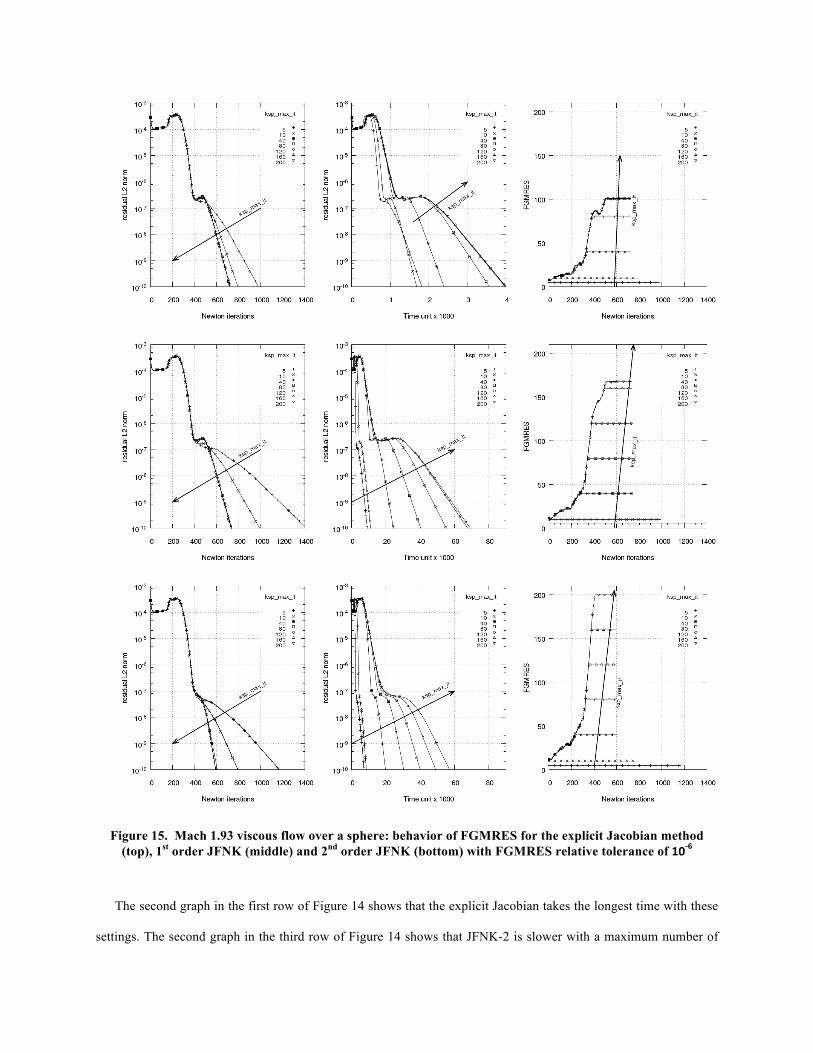
Figure 15. Mach 1.93 viscous flow over a sphere: behavior of FGMRES for the explicit Jacobian method (top), 1st order JFNK (middle) and 2nd order JFNK (bottom) with FGMRES relative tolerance of 10-6

The second graph in the first row of Figure 14 shows that the explicit Jacobian takes the longest time with these

settings. The second graph in the third row of Figure 14 shows that JFNK-2 is slower with a maximum number of

FGMRES iterations of 5 compared to 10. The second graph in the first row of Figure 15 shows that with lower

relative tolerance levels the explicit Jacobian is faster with maximum number of FGMRES iterations of 5 and 10,

however 10 is faster than 5. The above exceptions suggest that a maximum number of FGMRES iterations of 5 is

too small to ensure an appropriate convergence of the linear system.

It is also interesting to see that in the first columns of Figure 14 and Figure 15 that values of maximum number

of FGMRES iterations greater than 40 do not diminish the number of Newton iterations required for convergence,

but instead increase the number of FGMRES iterations (third column) and consequently dramatically increase the

wall time (second column). This analysis shows that in order to achieve an optimal computational time, it is

desirable to put a limit on the maximum number of FGMRES iterations and the relative tolerance in the convergence

of the unpreconditioned residual norm.

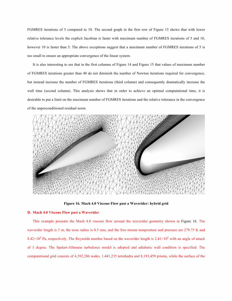
Figure 16. Mach 4.0 Viscous Flow past a Waverider: hybrid grid

D. Mach 4.0 Viscous Flow past a Waverider

This example presents the Mach 4.0 viscous flow around the waverider geometry shown in Figure 16. The

waverider length is 3 m, the nose radius is 0.5 mm, and the free-stream temperature and pressure are 279.75 K and

8.42×104 Pa, respectively. The Reynolds number based on the waverider length is 2.41×108 with an angle of attack

of 1 degree. The Spalart-Allmaras turbulence model is adopted and adiabatic wall condition is specified. The

computational grid consists of 4,392,286 nodes, 1,441,235 tetrahedra and 8,193,459 prisms, while the surface of the

waverider is discretized with 151,766 triangles. The initial CFL of 0.01 is exponentially increased to 10 in 1000

iterations. All the runs take 40 FGMRES iterations at every Newton step.

The Mach and density contours are shown in Figure 17. A detached bow shock is in front of the waverider and a

separation zone forms behind it. The speed-up diagram for 16, 32, 64 and 128 processors shown in Figure 18

highlights a 12% performance loss with 128 processors. The performance loss is due to the increase of the

communication cost as the number of processors increase.

Figure 17. Mach 4.0 Viscous Flow past a Waverider: Mach number contours (left) and density contours (right)

Figure 18. Mach 4.0 Viscous Flow past a Waverider: speedup diagram

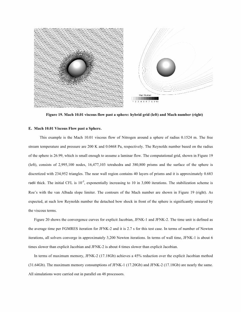
Figure 19. Mach 10.01 viscous flow past a sphere: hybrid grid (left) and Mach number (right)

E. Mach 10.01 Viscous Flow past a Sphere.

This example is the Mach 10.01 viscous flow of Nitrogen around a sphere of radius 0.1524 m. The free

stream temperature and pressure are 200 K and 0.0468 Pa, respectively. The Reynolds number based on the radius

of the sphere is 26.99, which is small enough to assume a laminar flow. The computational grid, shown in Figure 19

(left), consists of 2,995,100 nodes, 16,477,103 tetrahedra and 380,800 prisms and the surface of the sphere is

discretized with 234,952 triangles. The near wall region contains 40 layers of prisms and it is approximately 0.683

radii thick. The initial CFL is 10-5, exponentially increasing to 10 in 3,000 iterations. The stabilization scheme is

Roe’s with the van Albada slope limiter. The contours of the Mach number are shown in Figure 19 (right). As

expected, at such low Reynolds number the detached bow shock in front of the sphere is significantly smeared by

the viscous terms.

Figure 20 shows the convergence curves for explicit Jacobian, JFNK-1 and JFNK-2. The time unit is defined as

the average time per FGMRES iteration for JFNK-2 and it is 2.7 s for this test case. In terms of number of Newton

iterations, all solvers converge in approximately 3,200 Newton iterations. In terms of wall time, JFNK-1 is about 6

times slower than explicit Jacobian and JFNK-2 is about 4 times slower than explicit Jacobian.

In terms of maximum memory, JFNK-2 (17.18Gb) achieves a 45% reduction over the explicit Jacobian method

(31.64Gb). The maximum memory consumptions of JFNK-1 (17.20Gb) and JFNK-2 (17.18Gb) are nearly the same.

All simulations were carried out in parallel on 48 processors.

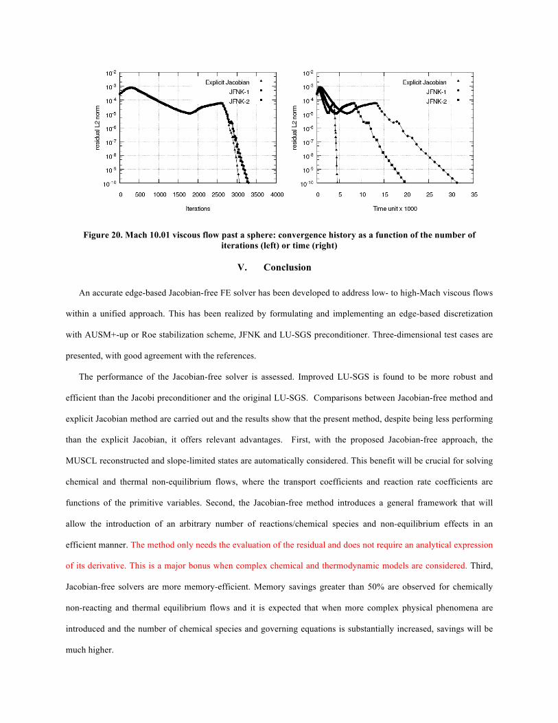
Figure 20. Mach 10.01 viscous flow past a sphere: convergence history as a function of the number of iterations (left) or time (right)

V. Conclusion

An accurate edge-based Jacobian-free FE solver has been developed to address low- to high-Mach viscous flows

within a unified approach. This has been realized by formulating and implementing an edge-based discretization

with AUSM+-up or Roe stabilization scheme, JFNK and LU-SGS preconditioner. Three-dimensional test cases are

presented, with good agreement with the references.

The performance of the Jacobian-free solver is assessed. Improved LU-SGS is found to be more robust and

efficient than the Jacobi preconditioner and the original LU-SGS. Comparisons between Jacobian-free method and

explicit Jacobian method are carried out and the results show that the present method, despite being less performing

than the explicit Jacobian, it offers relevant advantages. First, with the proposed Jacobian-free approach, the

MUSCL reconstructed and slope-limited states are automatically considered. This benefit will be crucial for solving

chemical and thermal non-equilibrium flows, where the transport coefficients and reaction rate coefficients are

functions of the primitive variables. Second, the Jacobian-free method introduces a general framework that will

allow the introduction of an arbitrary number of reactions/chemical species and non-equilibrium effects in an

efficient manner. The method only needs the evaluation of the residual and does not require an analytical expression

of its derivative. This is a major bonus when complex chemical and thermodynamic models are considered. Third,

Jacobian-free solvers are more memory-efficient. Memory savings greater than 50% are observed for chemically

non-reacting and thermal equilibrium flows and it is expected that when more complex physical phenomena are

introduced and the number of chemical species and governing equations is substantially increased, savings will be

much higher.

Acknowledgments

The authors acknowledge the financial support of the NSERC-Lockheed Martin Industrial Research Chair at the

McGill CFD Lab and through grant G238199 to ANSYS. We are grateful to Dr. Ned Allen, Chief Technologist,

Drs. Luke Uribarri and Ben Miller from Lockheed Martin for the continuous discussions and their industrial high-

TRL vision. ADD COMPUTE CANADA

References

1. Lee, J.H., Basic Governing Equations for the Flight Regimes of Aeroassisted Orbital Transfer Vehicles, in 19th Thermophysics Conference. 1984, American Institute of Aeronautics and Astronautics.

2. Barbante, P.F. and T.E. Magin, Fundamentals of hypersonic flight–properties of high temperature gases. RTO AVT Lecture Series on Critical Technologies for Hypersonic Vehicle Development, 2004: pp. 5.1-5.50.

3. Moses, P.L., et al., NASA hypersonic flight demonstrators—overview, status, and future plans. Acta Astronautica, 2004. 55(3): pp. 619-630.

4. Luo, H., J.D. Baum, and R. Löhner, A Fast, Matrix-free Implicit Method for Compressible Flows on Unstructured Grids. Journal of Computational Physics, 1998. 146(2): pp. 664-690.

5. Kirk, B.S., et al., Modeling Hypersonic Entry with the Fully-Implicit Navier–Stokes (FIN-S) Stabilized Finite Element Flow Solver. Computers & Fluids, 2014. 92(0): pp. 281-292.

6. Lani, A., An object oriented and high-performance platform for areothermodynamics simulations. Von Karman Institute for Fluid Dynamics, 2009.

7. Scalabrin, L.C., Numerical Simulation of Weakly Ionized Hypersonic Flow over Reentry Capsules. The University of Michigan, 2007.

8. Knoll, D.A. and D.E. Keyes, Jacobian-Free Newton-Krylov Methods: a Survey of Approaches and Applications. Journal of Computational Physics, 2004. 193(2): pp. 357-397.

9. Liu, L. and D.E. Keyes, Field-split preconditioned inexact newton algorithms. SIAM Journal on Scientific Computing, 2015. 37(3): pp. A1388-A1409.

10. Jameson, A. and S. Yoon, Lower-upper implicit schemes with multiple grids for the Euler equations. AIAA journal, 1987. 25(7): pp. 929-935.

11. Sharov, D. and K. Nakahashi, Reordering of hybrid unstructured grids for lower-upper symmetric gauss-seidel computations. AIAA Journal, 1998. 36(3): pp. 484-486.

12. Landau, L.D. and E.M. Lifshitz, Fluid Mechanics. 1959, Oxford: Pergamon Press. 13. Aris, R.X., Vectors, tensors and the basic equations of fluid mechanics. 2012: Courier Corporation. 14. Selmin, V., The Node-centred Finite Volume Approach: Bridge Between Finite Differences and Finite Elements.

Computer Methods in Applied Mechanics and Engineering, 1993. 102(1): pp. 107-138. 15. Liou, M.-S., A Sequel to AUSM: AUSM+. Journal of Computational Physics, 1996. 129(2): pp. 364-382. 16. Roe, P.L., Approximate Riemann solvers, parameter vectors, and difference schemes. Journal of computational physics,

1981. 43(2): pp. 357-372. 17. Barth, T.J., Aspects of unstructured grids and finite-volume solvers for the Euler and Navier-Stokes equations. Notes

for VKI Lecture Series, 1992: pp. 105. 18. Löhner, R. and M. Galle, Minimization of indirect addressing for edge‐based field solvers. Communications in

numerical methods in engineering, 2002. 18(5): pp. 335-343. 19. Selmin, V. and L. Formaggia, Simulation of hypersonic flows on unstructured grids. International journal for numerical

methods in engineering, 1992. 34(2): pp. 569-606. 20. Van Leer, B., Towards the ultimate conservative difference scheme. V. A second-order sequel to Godunov's method.

Journal of computational Physics, 1979. 32(1): pp. 101-136. 21. Venkatakrishnan, V., Convergence to steady-state solutions of the Euler equations on unstructured grids with limiters.

Journal of computational physics, 1995. 118(1): pp. 120-130. 22. Hou, J., F. Simons, and R. Hinkelmann, Improved total variation diminishing schemes for advection simulation on

arbitrary grids. International Journal for Numerical Methods in Fluids, 2012. 70(3): pp. 359-382. 23. Jameson, A., Time dependent calculations using multigrid, with applications to unsteady flows past airfoils and wings.

AIAA paper, 1991. 1596: pp. 1991.

24. Saad, Y., A flexible inner-outer preconditioned GMRES algorithm. SIAM Journal on Scientific Computing, 1993. 14(2): pp. 461-469.

25. Eisenstat, S.C. and H.F. Walker, Choosing the Forcing Terms in an Inexact Newton Method. SIAM Journal on Scientific Computing, 1996. 17(1): pp. 16-32.

26. Carpentieri, G., An adjoint-based shape-optimization method for aerodynamic design. 2009: TU Delft, Delft University of Technology.

27. Balay, S., et al. Petsc web page. 2016; Available from: http://www.mcs.anl.gov/petsc. 28. Rumsey, C.L., et al., Summary of the first AIAA CFD high-lift prediction workshop. Journal of Aircraft, 2011. 48(6):

pp. 2068-2079. 29. Remaki, L., et al. On the a Posteriori Error Estimation in Mesh Adaptation to Improve CFD Solutions. in 44rd AIAA

Aerospace Sciences Meeting and Exhibit. 2006. 30. Schmitt, V. and F. Charpin, Pressure distributions on the ONERA-M6-wing at transonic Mach numbers. Experimental

data base for computer program assessment, 1979. 4. 31. Qin, N., D.K. Ludlow, and S.T. Shaw, A matrix‐free preconditioned Newton/GMRES method for unsteady Navier–

Stokes solutions. International Journal for Numerical Methods in Fluids, 2000. 33(2): pp. 223-248. 32. Gnoffo, P.A., Forebody and afterbody solutions of the Navier-Stokes equations for supersonic flow over blunt bodies in

a generalized orthogonal coordinate system. NASA TP-107, 1978. 33. Venkatakrishnan, V. and D.J. Mavriplis, Implicit solvers for unstructured meshes. Journal of computational Physics,

1993. 105(1): pp. 83-91