a hybridized discontinuous petrov–galerkin scheme for scalar...

INTERNATIONAL JOURNAL FOR NUMERICAL METHODS IN ENGINEERINGInt. J. Numer. Meth. Engng 2012; 91:950–970Published online 13 June 2012 in Wiley Online Library (wileyonlinelibrary.com). DOI: 10.1002/nme.4300

A hybridized discontinuous Petrov–Galerkin scheme for scalarconservation laws

D. Moro*,†, N. C. Nguyen and J. Peraire

Department of Aeronautics and Astronautics, Massachusetts Institute of Technology, Cambridge, MA, USA

SUMMARY

We present a hybridized discontinuous Petrov–Galerkin (HDPG) method for the numerical solution of steadyand time-dependent scalar conservation laws. The method combines a hybridization technique with a localPetrov–Galerkin approach in which the test functions are computed to maximize the inf-sup condition.Since the Petrov–Galerkin approach does not guarantee a conservative solution, we propose to enforce thisexplicitly by introducing a constraint into the local Petrov–Galerkin problem. When the resulting nonlinearsystem is solved using the Newton–Raphson procedure, the solution inside each element can be locallycondensed to yield a global linear system involving only the degrees of freedom of the numerical trace. Thisresults in a significant reduction in memory storage and computation time for the solution of the matrixsystem, albeit at the cost of solving the local Petrov–Galerkin problems. However, these local problems areindependent of each other and thus perfectly scalable. We present several numerical examples to assess theperformance of the proposed method. The results show that the HDPG method outperforms the hybridizablediscontinuous Galerkin method for problems involving discontinuities. Moreover, for the test case proposedby Peterson, the HDPG method provides optimal convergence of order kC1. Copyright © 2012 John Wiley& Sons, Ltd.

Received 5 October 2011; Revised 17 January 2012; Accepted 27 January 2012

KEY WORDS: hybridized discontinuous Galerkin; Petrov–Galerkin; nonlinear conservation laws

1. INTRODUCTION

The development of robust, accurate, and efficient methods for the numerical solution ofconservation laws in complex geometries is a topic of considerable importance. Indeed, hyperbolicsystems of conservation laws govern a wide range of physical phenomena and arise in severalareas of applied mathematics and mechanics such as fluid dynamics, thermodynamics, populationdynamics, magnetohydrodynamics, multiphase flow in nonlinear material, and traffic flow. The mostfundamental phenomenon of hyperbolic systems is the formation and propagation of discontinuitiesand shock waves even if initial and boundary data are smooth. The presence of shock waves isa serious challenge for any numerical methods to provide a physical and stable solution. Althoughsignificant progress has been made over the years in both the theoretical and numerical investigation,the numerical solution of hyperbolic conservation laws remains an active research area with manychallenging problems to be addressed.

In recent years, considerable attention has been turned to discontinuous Galerkin (DG) methods[1–13] for the numerical solution of hyperbolic conservation laws. DG methods possess severalattractive properties for solving hyperbolic problems. In particular, they are flexible for complicatedgeometry, locally conservative, high-order accurate, highly parallelizable, and have low dissipationand dispersion. However, most existing DG methods suffer from two major drawbacks. The first

*Correspondence to: D. Moro, 77 Massachusetts Ave. 37-422 Cambridge MA 02139, USA.†E-mail: [email protected]

Copyright © 2012 John Wiley & Sons, Ltd.

HDPG SCHEME FOR SCALAR CONSERVATION LAWS 951

drawback is that they are computationally expensive due to the large number of degrees of freedom(DOFs) caused by nodal duplication at the element boundary interfaces. The memory storage andcomputation cost of DG methods are typically several times greater than that of CG methods. Thesecond drawback is that higher-order DG methods are generally less robust than low-order methodswhen solution features are under-resolved (in particular at shock waves).

More recently, a new class of implicit DG methods—the so-called hybridizable discontinuousGalerkin (HDG) method—was first introduced for elliptic problems [14]. The HDG methodshave already been extended to convection–diffusion systems [15, 16], linear and nonlinearelastodynamics [17,18], incompressible and compressible flows [19–26], and electromagnetics [27].The main idea of HDG methods is a hybridization of DG methods, which aims to solve for thenumerical trace of the approximate solution instead of the approximate solution itself. Becausethe numerical trace is defined over inter-element boundaries and is single-valued over the elementfaces, HDG methods have significantly less DOFs than standard DG methods. In fact, a variantof the HDG method—the so-called embedded DG method [28, 29]—has the same global DOFs asCG methods and has the stability properties of a DG method. This large reduction in the numberof DOFs can lead to significant savings for both computational time and memory storage. Anotheradvantage of HDG methods is that their post-processed solution and approximate gradient convergewith one order higher than those of other DG and CG methods for diffusion-dominated problems.These advantages render HDG methods competitive with CG methods even for diffusion problemsand elasticity problems [15, 17, 18, 30].

Another interesting DG approach is the discontinuous Petrov–Galerkin method (DPG) firstintroduced for convection problems [7] and later extended to linear convection–diffusion problems[31]. The main idea of the DPG method is an automatic construction of optimal test functions tomaximize the stability constant. The performance of the DPG method is shown to be superior tothe standard DG method. In particular, the DPG method delivers optimal convergence rate k C 1for the Peterson example, where it has been known that other DG methods yield a convergence rateof only k C 1=2. The stability of the DPG scheme is excellent. However, the DPG method is moreexpensive than other DG methods because it contains more globally coupled unknowns. Anotherdrawback of the DPG method is that the method is not conservative because its test space does notcontain a constant function.

In this paper, we introduce a hybridized discontinuous Petrov–Galerkin (HDPG) method thatcombines the efficiency of the HDG method with the excellent stability of the DPG method. Themain idea here is to use the DPG method for the local problem and the HDG method for the globalproblem. The global unknown and in fact the matrix structure of the HDPG method is thus thesame as that of the HDG method. Moreover, in order to render the HDPG method conservative,we propose to enrich the test space with a constant function by introducing a constraint intothe local problem. We present several numerical examples to demonstrate the performance of theHDPG method. Numerical results show that the HDPG method is more robust and stable than theHDG method for a number of test cases. Moreover, for the test case proposed by Peterson [32],the HDPG method provides optimal convergence of order kC 1.

The paper is organized as follows. In Section 2, we introduce some notation used throughout thepaper and present a brief overview of both the HDG method and the DPG method. We then describethe HDPG method in Section 3 and present numerical results in Section 4. Finally, in Section 5, wedraw some concluding remarks.

2. OVERVIEW

2.1. Problem statement and notation

We first introduce the problem of interest, which is a scalar conservation law of the following form:

r � F.u/�r � .�ru/D f , in �,

uD gD , on @�.(1)

Copyright © 2012 John Wiley & Sons, Ltd. Int. J. Numer. Meth. Engng 2012; 91:950–970DOI: 10.1002/nme

952 D. MORO, N. C. NGUYEN AND J. PERAIRE

As usual in the DG context, the problem is written as a first-order system:

r � F.u/�r � .�q/D f , in �,

q�ruD 0, in �,

uD gD , on @�.

(2)

Here, � 2 Rd is the physical domain in d spatial dimensions with Lipschitz boundary @�,f 2 L2.�/ is a square integrable source term, � 2 L1.�/ represents the isotropic diffusioncoefficient, and gD 2 L2.@�/ represents the boundary data. Moreover, u 2 L2.�/ representsthe scalar field, and F.u/ 2 .L1.�//d is a vector-valued function of the solution u.

Let Th denote a collection of disjoint elements K that partition the domain �. Let @Th denotethe set of faces of the triangulation Th, formed by collecting the faces of each element K, this is,@Th WD ¹@K WK 2 Thº. For a given element of the triangulation K, e D @K \ @� is a boundaryface if its d � 1 Lebesgue measure is non-zero. Similarly, for two elements KC and K� of thetriangulation, e D @KC \ @K� is an interior face if its d � 1 Lebesgue measure is non-zero. Let E i

h

denote the set of interior faces and E@h

denote the set of boundary faces. We denote by Eh WD E ih[E@

h

the union of both sets. Notice that each interior face in E ih

is represented twice in @Th, whereas eachboundary face in E@

his represented only once. Finally, let nC and n� denote the outward unit normal

for element KC and K�, respectively. Notice, by definition, if KC and K� share a face e of Eh,then nC D�n�.

Let Pp.D/ denote the set of polynomials of order at most p in a domain D. We define the finiteelement spaces as follows:

Vp

hD®v 2 L2.Th/ W vjK 2 Pp.K/ 8K 2 Th

¯,

Wp

hD°

w 2 .L2.Th//d W wjK 2 .Pp.K//d 8K 2 Th±

,

Mp

hD®� 2 L2.Eh/ W �je 2 Pp.e/ 8e 2 Eh

¯,

that are polynomials inside each element (in the case of V ph

and Wp

h) or face (in the case of Mp

h),

but discontinuous across them. We also define Mp

h.gD/ D ¹� 2 M

p

hW � D P.gD/º, where P.�/

denotes the L2 projection of the given data .�/ on Mp

h.

Finally, we define the following inner products as follows:

.a, b/Th DXK2Th

.a, b/K , .a, b/Th DXK2Th

dXiD1

.ai , bi /K ,

ha, biEh DXe2Eh

ha, bie , ha, bi@Th DXK2Th

ha, bi@K ,

where, for any functions a, b 2 L2.D/, we define .a, b/D DRDab ifD 2Rd and ha, biD D

RDab

if D 2Rd�1.

2.2. HDG Scheme

Given an element K of the triangulation Th, let Ou be a function supported on @K. We introduce theso-called local problem as follows:

r � F�u Ou��r �

��q Ou

�D f , in K,

q Ou �ru Ou D 0, in K, (3)

u Ou D Ou, on @K.

The local problem defines a Dirichlet-to-Neumann mapping T W Ou 7!�

F�u Ou�� q Ou

��n that maps

boundary data Ou to the fluxes on @K. It is clear that if Ou D uj@K , then, we have q Ou D q,u Ou D u.



However, Ou is unknown unless an extra condition is prescribed. Thanks to the conservative characterof the equation, we can impose that jumps in the fluxes across faces must be zero in the interior,together with the appropriate boundary condition:�

F�u Ou�� q Ou

�Ce� nCC

�F�u Ou�� q Ou

��e� n� D 0, 8e 2 E ih,

OuD gD , 8e 2 E@h .(4)

This equation gives rise to the global system in terms of Ou because .u Ou, q Ou/ is a function of Ou by(3). The discrete version of the system (3)–(4) defines the HDG method.

As we discuss later, depending on the choice of the approximation space, several HDGschemes can be devised [14]. In this particular case, we take the usual DG spaces consisting ofpiecewise polynomials of the same order p for all the unknowns. Multiplying (3)–(4) by testfunctions, and integrating by parts over each element or face, we arrive at the following weakformulation for the approximate solution; find .uh, qh, Ouh/ 2 V

p

h�Wp

h�M

p

h.gD/ such that

h�OFh � � Oqh

�� n, vi@K � .F.uh/� �qh,rv/K D .f , v/K ,

.qh, w/K C .uh,r �w/K � h Ouh, w � ni@K D 0, (5)

h�OFh � � Oqh

�C� nCC . OFh � � Oqh/

� � n�,�ie D 0,

for allK 2 Th, all e 2 E ih

and all .v, w,�/ 2 V ph�Wp

h�M

p

h.0/. Owing to the discontinuous nature

of the approximation spaces, the integration by parts introduces the so-called numerical fluxes OFhand Oqh that represent an approximation to the fluxes at the interfaces and have to satisfy certainproperties to render the system well posed.

By summing (5) over all the elements, the problem reads as follows: find .uh, qh, Ouh/ 2Vp

h�Wp

h�M

p

h.gD/ such that

h�OFh � � Oqh

�� n, vi@Th � .F.uh/� �qh,rv/Th D .f , v/Th , 8v 2 V p

h,

.qh, w/Th C .uh,r �w/Th � h Ouh, w � ni@Th D 0, 8w 2Wp

h,

h�OFh � � Oqh

�� n,�i@Th D 0, 8� 2M

p

h.0/,

(6)

where the numerical fluxes are given by

OFh � � Oqh D F . Ouh/� �qhC � .uh, Ouh/ .uh � Ouh/ � n. (7)

Here, �.uh, Ouh/ is the stabilization parameter. The choice of � is vital for the system to be wellposed. A detailed analysis can be found in [16] and yields the following condition, that requiresF.u/ to be a differentiable function of u:

� >�

lC1

2sup jF0.s/ � nj, s 2 Œmin¹uh, Ouhº, max ¹uh, Ouhº� , (8)

where l is a characteristic length of the problem and the second term is related to the maximumwave speed across interfaces. For the cases of interest in this paper, a constant value of � will bechosen big enough to satisfy (8).

2.3. DPG Scheme

2.3.1. Optimal test functions. We will now describe the theory of the optimal test functionsfirst introduced by Demkowicz and Gopalakrishnan in the series of papers [7, 31, 33] for linearconvection–diffusion equations. Towards this end, we consider an abstract weak formulation: findu 2 U such that

b.u, v/D l.v/, 8v 2 V , (9)



where U and V are Hilbert spaces, b.�, �/ W U �V 7!R is a continuous bilinear form, and l.�/ 2 V 0 isan element of the dual space of V . It is well known that the existence and uniqueness of the solutionof this problem is associated with the so-called inf-sup constant � (Babuska, [34]):

� WD infu2U

supv2V

b.u, v/

kukU kvkV, (10)

in particular, if � > 0, then problem 9 has a unique solution.In the finite element context, we replace U with Uh and V with Vh, where Uh and Vh are suitable

finite element spaces. As a result, we arrive at the following problem: find uh 2 Uh such that

b.uh, vh/D l.vh/, 8vh 2 Vh. (11)

The discrete inf-sup constant is then defined as

�h WD infuh2Uh

supvh2Vh

b.uh, vh/

kuhkU kvhkV, (12)

and plays exactly the same role as the continuous one (10) in the sense that �h > 0 is required forexistence and uniqueness. Our interest resides in using trial spaces Uh with good approximationproperties (e.g., polynomials of order p), and computing the tests space Vh so that the stabilityconstant �h is maximized. As described in [31], this can be achieved when the test functions arecomputed using the composition of the operator that defines the problem and the inverse Rieszmapping to yield T W Uh 7! V . The test space is obtained using the auxiliary problem: find Tei 2 Vsuch that:

.Tei , v/V D b.ei , v/, 8v 2 V , (13)

for each basis function of the trial space ei (Uh D span¹eiº). The discrete test space is then taken asVh D span¹Teiº.

2.3.2. DPG formulation. In practice, the previous step involves the non-trivial task of invertinga continuous operator; hence, some degree of discretization has to be introduced. The approachproposed in [7, 31, 33] relies on a space of candidate test functions QVh based on polynomials oforder pC�p. This way, the approximate trial-to-test map reads: find Thei 2 QVh such that

.Thei , v/V D b.ei , v/, 8v 2 QVh. (14)

The biggest obstacle becomes the inversion of the metric of the inner product .�, �/V for the basisof QVh. It is clear that in the case where continuous finite element spaces are used, the continuity ofthe basis functions across elements generates a metric with a sparsity pattern similar to the originalbilinear form; hence, as expensive to solve as the weak formulation itself. However, when no suchcontinuity conditions appear between elements, as in the case of the usual DG spaces, the metriccan be efficiently inverted element-wise.

This is the basic approach proposed in [7, 31, 33], where the discontinuous Petrov–Galerkinscheme of Bottasso et al. [35] is used in combination with the approximate optimal test functionsdescribed here. Finally, note the choice of the space QVh is not unique and several other approachescould be used, e.g. bubbles, provided dim. QVh/ > dim.Uh/. In any case, the use of higher orderpolynomials seems to be the most cost-effective solution as we would expect the approximate testspace to converge towards the optimal one (in the sense of (13)) as �p is increased.

3. HYBRIDIZED DISCONTINUOUS PETROV–GALERKIN SCHEME

3.1. Nonlinear optimal test functions

We extend the previous theory to nonlinear conservation laws. For that, the theory has to be extendedto the case of a nonlinear weak formulation: find u 2 U such that

a.u, v/D l.v/, 8v 2 V , (15)



where the operator a.�, �/ W U � V 7! R is linear in v (indeed a.u, �/ 2 V 0), but nonlinear in u. Inthis case, the problem can be usually written in residual form as follows: find u 2 U such that

r.u, v/ WD a.u, v/� l.v/D 0, 8v 2 V . (16)

Note that the operator r is linear in v. The discrete approximation then reads as follows: find uh 2 Uhsuch that

r.uh, v/D 0, 8v 2 Vh. (17)

The test space Vh is constructed as follows.Following the spirit of the previous section, we will assume that the test functions are not

known a priori and will be selected from a certain space QVh that satisfies dim�QVh�> dim.Uh/. In

particular, one can use a similar approach to compute the test functions by means of the followingtrial-to-test map:

.Thei , v/V D r0uh.ei , v/, 8v 2 QVh, (18)

where r 0uh.w, v/ is the bilinear form induced by the Frechet derivative of r.u, v/ with respect to uevaluated at uh. The discrete test space is then taken as Vh D span¹Teiº. It is important to pointout that in the nonlinear case, the test space Vh depends on uh because r 0uh.w, v/ depends on uh.Therefore, the test functions can not be computed in advance as in the linear case.

We would like to point out a main difference between the proposed approach and the original DPGscheme introduced in [36] for nonlinear problems. Our approach applies the concept of optimal testfunctions to the nonlinear residual r.u, v/, whereas the DPG scheme applies this concept to thelinearized problem arising from the Newton iteration on the nonlinear system. In other words, ourapproach is Petrov–Galerkin projection followed by linearization, whereas the original DPG schemeis linearization followed by Petrov–Galerkin projection. Hence, the test functions generated by theoriginal DPG approach are optimal with respect to the linearized problem, but not to the originalnonlinear problem. Owing to this lack of consistency in the Jacobian, the DPG scheme suffers fromslow convergence (as reported in [36]) in some cases.

Proposition 1The nonlinear weak formulation (17) solved using the approximate optimal test space from (18) isequivalent to the solution of the following problem:

uh D arg infwh2Uh

supv2 QVh

r.wh, v/

kvkV. (19)

ProofLet v 2Rn denote the vector of coefficients of an element vh 2 QVh. Similarly, let u 2Rm (w 2Rm)denote the vector of coefficients of an element uh 2 Uh (wh 2 Uh, respectively). We can rewrite themin–max statement as follows:

uD arg minw2Rm

maxv2Rn

vT r.w/pvTXV v

, (20)

where the vector r.w/ represents the usual duality pairing r D r.wh, v/ against each element of thebasis for QVh, and XV represents the metric of the space QVh. The inner maximization statement canbe solved exactly using the first order optimality condition:

r.w/pvTXV v

�vT r.w/�

vTXV v�3=2XV vD 0) vD

�vTXV v

� X�1V r.w/

vT r.w/. (21)

The solution to the problem is unique (up to a scaling of v) as one can prove by rewriting it withthe additional constraint kvkV D 1, in which case, the objective is linear with convex constraints.Inserting (21) into (20), we obtain the following:

uD arg minw2Rm

qr.w/TX�1V r.w/. (22)



The first order optimality condition for (22) yields

1

2q

r.u/TX�1V r.u/

@r.u/@u

T

X�1V r.u/D 0)@r.u/@u

T

X�1V r.u/D 0, (23)

to form a system of nonlinear equations for u.To show the equivalence, we take (17) and write it in discrete form as follows: find u 2 Rm

such that

vT r.u/D 0, 8v 2 QVh. (24)

Here, QVh D span¹ti , 16 i 6mº is obtained using the mapping defined in (18): find ti 2Rn such that

ti DX�[email protected]/@u

ei , (25)

where ei denotes the vector of coefficients of ei 2 Uh. Combining (24) and (25), we obtain

[email protected]/@u

T

X�1V r.u/D 0, 8w 2Rm. (26)

The desired result follows directly from (22) and (26). �

Remark 1The minimization statement (22) can also be written as follows:

uD arg minw2Rm

1

2r.w/TX�1V r.w/, (27)

which represents a very general and flexible point of departure. In particular, it can be easilyconstrained to guarantee certain properties such as local conservation.

3.2. HDPG formulation

A limitation of the DPG scheme presented in [31,33,36] is the fact that the DPG system is formed bymultiplying the transposed Jacobian by itself, hence, yielding a denser system to solve. Furthermore,the scheme is not conservative in the sense that the constant mode is not guaranteed to belong to theoptimal test space. Despite these limitations, the scheme has certain good properties. For example,it is clear that in the case of linear equations, the final system to solve for is symmetric positive-definite and hence can be efficiently solved using well-developed iterative algorithms such as theconjugate gradients method. Moreover, the DPG scheme gives optimal p C 1 error convergencefor the well-known case proposed by Peterson [32], whereas other DG methods can only achievepC 1=2 error convergence.

Our goal in this paper is to propose a new scheme that

� preserves the efficiency of the HDG scheme;� incorporates the excellent stability of the DPG scheme; and� enforces conservative solutions.

To define the HDPG scheme, we first introduce the residuals associated with the HDG formulation(6)–(7) as

rKu .ah, bh, vI Oah/DhF . Oah/ � n� �bh � nC � .ah, Oah/ .ah � Oah/ , vi@K� .F.ah/� �bh,rv/K � .f , v/K ,

rKq .ah, bh, wI Oah/D .bh, w/K C .ah,r �w/K � hOah, w � ni@K , (28)

r Ou .ah, bh, Oah,�/DhF . Oah/ � n� �bh � nC � .ah, Oah/ .ah � Oah/ ,�i@Th ,

where we have inserted the definition of the numerical fluxes (7) into (6).



The HDPG formulation then reads as follows: find Ouh 2Mp

h.gD/ such that

r Ou.uh, qh, Ouh,�/D 0, 8� 2Mp

h.0/, (29)

where .uh. Ouh/, qh. Ouh//jK 2 Pp.K/� .Pp.K//d satisfies the following:

.uh. Ouh/, qh. Ouh//jK D arg inf.ah,bh/2Pp.K/�.Pp.K//d

�max

v2PpC�p.K/

rKu .ah, bh, vI Ouh/

kvkV

�,

s.t. rKq .ah, bh, wI Ouh/D 0, 8w 2 .Pp.K//d

s.t. rKu .ah, bh, 1I Ouh/D 0,

(30)

for all K 2 Th. The system (29)-(30) completes the definition of the HDPG scheme.Some remarks about the HDPG scheme are in order. The first equation (29) weakly enforces the

continuity of the normal component of the numerical fluxes across elemental interfaces whereasthe second equation (30) defines .uh, qh/ as a function of Ouh locally on every element. Therefore,(29) is called the global problem, which gives rise to a nonlinear algebraic system for the DOFs of Ouhonly. As for the local problem (30), we apply the optimal test function approach to the conservationlaw only and strongly impose an equality constraint on the kinematic relationship by requiring thatrKq .ah, bh, wI Ouh/ D 0, 8w 2 .Pp.K//d . In addition, we explicitly enforce the conservation ofthe HDPG scheme at the local level by requiring the integration against a constant test functionv 2 P0.K/ to be strongly satisfied.

3.3. Solution procedure

Our focus now is the solution of system (29)–(30). We shall seek an iterative algorithm that takesadvantage of the definition of the local problem to solve for the globally coupled DOFs of Ouhonly. In particular, we apply the Newton–Raphson method to the global problem (29), therebyobtaining a linear system at each iteration. This, in turn, requires us to solve the local problem (30)for .uh. Ouh/, qh. Ouh// and the associated sensitivities.

3.3.1. Algebraic system. Some further notation is required before introducing the iteration. Wedenote by .u, Q, Ou/ the vectors of coefficients associated with the functions .uh, qh, Ouh/ 2 V

p

h�

Wp

h�M

p

h.gD/. We also denote by rKu , rKq and r Ou the residual vectors associated with rKu , rKq and

r Ou, respectively (see Appendix for description). This allows us to rewrite the HDPG formulation(29)–(30) as an algebraic system: find Ou 2Rn such that

r Ou.u, Q, Ou/D 0 (31)

where .u. Ou/, Q. Ou//jK 2Rm �Rm�d satisfies

.u, Q/jK D arg min.a,B/2Rm�Rm�d

1

2rKu .a, BI Ou/TX�1V rKu .a, BI Ou/,

s.t. rKq .a, BI Ou/D 0,

s.t. cT rKu .a, BI Ou/D 0,

(32)

for all K 2 Th, where c is the vector of coefficients for the constant mode represented in the localbasis for PpC�p.K/.

3.3.2. Global solver. As indicated earlier, in order to solve the system (31), we will use a Newton–

Raphson iteration. For this, given a current iterate�Nu, NQ, NOu

�that satisfies the local problem�

Nu, NQ� ˇ̌̌K D

�u�NOu�

, Q�NOu��ˇ̌̌

K, we seek updates to the solution ı Ou by solving the following system:�@r Ou@ OuC@r Ou@u

@u@ OuC@r Ou@Q

@Q@ Ou

�ı OuD�r Ou, (33)



where we have used the chain rule to obtain the fully linearized system with respect to Ou. Here,all the terms involved such as residuals or Jacobians have to be computed using the current iterate�Nu, NQ, NOu

�. More details on the computation of these can be found in Appendix A. The iteration

is repeated in the usual Newton–Raphson fashion until the update gets below a certain tolerance(kı Ouk < tol). To avoid the divergence of the iteration, a damped Newton strategy is implementedthat limits the stepsize by ˛ 6 1 to guarantee kr Ou. Ou/k > kr Ou. OuC ı Ou/k. The choice of ˛ followsthe usual bisection rule. After each iteration, we use ˛ı Ou to update the solution. A basic algorithmicdescription can be found later.

In theory, we would expect the Newton–Raphson iteration to present quadratic convergence oncethe iterate is close to the solution. For this, the Jacobian matrix has to be properly computed, this

meaning, we require the dependencies�Nu, NQ

� ˇ̌̌K D

�u�NOu�


Kand the sensitivities @u=@ Ou

and @Q=@ Ou to be solved exactly (up to numerical error).

3.3.3. Exact local solver. We now describe an iterative scheme to solve the local problem (32) and

obtain the desired dependencies�Nu, NQ

� ˇ̌̌K D

�u�NOu�


K. For this, two different approaches

will be combined using a simple switch. The first approach is to linearize the different residualsthat enter the problem before taking any minimization step. By this, we mean, from a current iterateNZ D

�Nu, NQ

�, we look for updates ıZ D .ıu, ıQ/ that solve the following linearized problem: given

Ouh 2Mp

h, find ıZ 2Rm �Rm�d such that

ıZD arg minıC2Rm�Rm�d

1

2

�rKu C

@rKu@Z

ıC�T

X�1V

�rKu C

@rKu@Z

ıC�

,

s.t rKq C@rKq@Z

ıCD 0,

s.t cT�

rKu C@rKu@Z

ıC�D 0,

(34)

where the different terms that appear in this system are described in Appendix A. Notice that thevariable NZ has been introduced to simplify the notation. The minimization now follows by derivingthe Karush–Kuhn–Tucker conditions for ıZ:

26666664

�@rKu@Z

�TX�1V

�@rKu@Z

�@rKq@Z

T �@rKu@Z

�Tc

@rKq@Z 0 0

cT�@rKu@Z

�0 0

377777758<:ıZ�

9=;D�

8̂̂̂<ˆ̂̂:

�@rKu@Z

�TX�1V rKu

rKq

cT rKu

9>>>=>>>;

. (35)

Notice how Ouh is fixed and just acts as a parameter. Also notice that plays the role of aLagrange multiplier for the conservation whereas � represents a set of Lagrange multipliers forthe kinematic variables. This approach represents a constrained version of the well-known Gauss–Newton method (GN) for nonlinear least squares problems. The GN method is very robust inthe sense that at each iteration, the computed update is a feasible descent direction of the prob-lem. Also, it is well known that the convergence of this scheme can approach a quadratic rate,though this strongly depends on the value of the objective function at convergence. In partic-ular, when it is non-zero, some terms are missing in the linearization that may slow or evenprevent convergence.



The second approach to solve (32) is to depart from the first order optimality conditions directly:�@rKu@Z

�TX�1V rKu C�

T

@rKq@Z

!C cT

�@rKu@Z

�D0,

rKq D0, (36)

cT rKu D0,

and apply the Newton–Raphson iteration to it. This is also known as sequential quadraticprogramming (SQP) and yields the following system to solve2

6666664

�@rKu@Z

�TX�1V

�@rKu@Z

�C�@2rKu@Z2

��X�1V rKu C cT

� @rKq@Z

T �@rKu@Z

�Tc

@rKq@Z 0 0

cT�@rKu@Z

�0 0

377777758<:ıZ�

9=;D

�

8̂̂̂<̂ˆ̂̂̂:

�@rKu@Z

�TX�1V rKu

rKq

cT rKu

9>>>>=>>>>;

, (37)

where the vector of unknowns contains the update ıZ and the approximate Lagrange multipliers.This way, the difference between (35) and (37) is only the second derivative terms that appear in thelatter one. These derivatives account for the variation of the test space with respect to the solutionand play a vital role in the convergence. Indeed, this might be the reason why the DPG schemeof [36] does not achieve quadratic convergence even once close to the solution (see [36] pp. 16).Notice also the second derivatives of rKq have not been included since this residual is linear in allthe arguments.

One of the most important properties of the SQP iteration is the rate of convergence, which islocally quadratic when close enough to the solution. Its main disadvantage is the cost associatedwith constructing the second derivatives. Hence, we propose to combine the Gauss–Newton withthe SQP in order to take advantage of their respective properties. In particular, we propose a switchof schemes based on the size of the update kıZk. More sophisticated switches might be devised,but this works fine for the cases of interest here. The local solver iteration is described in thealgorithm below.

Before moving on to the next step in the HDPG scheme, we would like to comment on the localsolver just presented. In particular, we would like to point out that the problem to solve (32) is ofthe constrained nonlinear least squares kind. These problems have long been studied in the fieldof optimization; hence, very efficient algorithms exist to solve them (e.g., Levenberg–Marquardtalgorithm). We did not explore other options than the two presented here, which proved to be veryefficient at solving all types of elements, even with strongly under-resolved shocks in them as wewill see in the Results section.

From an implementation point of view, the local solver cost can be reduced if the equations for thekinematic relationships are inverted before the minimization takes place. Namely, one can see from(28) that the relationship between these variables is linear, and more importantly, can be invertedlocally to obtain qh D qh.uh, Ouh/. This way, the minimization statement only involves uh and Ouh,and the Lagrange multipliers � can be dispensed with.

3.3.4. Local problem sensitivities @uh@ Ouh

, @qh@ Ouh

. Once the local problem is solved, the sensitivities ofthe local solution to the boundary data, required to formulate system (33) have to be computed. Todo so, we can use the first order optimality conditions, (36), and use the implicit function theorem



to obtain the sensitivities. For this, let NOU 2 Rt�f be the coefficients of Ouh on @K, where f is thenumber of faces. The system to solve for the sensitivities reads as follows:2

6666664

�@rKu@Z

�TX�1V

�@rKu@Z

�C�@2rKu@Z2


� @rKq@Z

T �@rKu@Z

�Tc

@rKq@Z 0 0

cT�@rKu@Z

�0 0

37777775

8̂̂̂<̂ˆ̂̂̂:

@Z@ OU

@

@ OU

@�

@ OU

9>>>>=>>>>;D

�

8̂̂̂ˆ̂<ˆ̂̂̂̂:

�@rKu@Z

�TX�1V

�@rKu@ OU

�C�@2rKu@Z@ OU


�@rKq@ OU

cT @rKu@ OU

9>>>>>=>>>>>;

, (38)

where the different terms that appear are properly described in Appendix A. Notice that the onlycondition for this to hold is that the Jacobian of the implicit mapping with respect to the variablewe want to compute sensitivities for, has to be invertible. Notice this is just the matrix on the leftof (38), that coincides with the matrix from the SQP iteration, and because of this, can be reusedprovided the convergence tolerance for the local solver is small enough to make the changes inthe solution negligible. Our test indicates this strategy does not affect the overall convergence ofthe scheme.



3.4. Extension to time dependent problems

Next, we would like to extend the HDPG scheme to an unsteady convection–diffusion problemdefined by the following:

@u

@tCr � F.u/�r � .�q/D f , in �,

q�ruD 0, in �,

uD gD , on @�.

(39)

In particular, we introduce the usual polynomial spaces for the solution; however, we assumethis solution is parameterized by the time t . Namely, we seek .uh.t/, qh.t/, Ouh.t// 2 V

p

h�Wp

h�

Mp

h.gD/. We can derive the weak formulation residuals by using integration by parts as follows:

ruK.uh, qh, vI Ouh/D

�@uh

@t, v

�K

C hF. Ouh/ � nC �qh � nC �.uh, Ouh/.uh � Ouh/, vi@K

� .F.uh/� �qh,rv/K � .f , v/K , (40)

rqK.uh, qh, wI Ouh/D .qh, w/K C .uh,r �w/K � h Ouh, w � ni@K ,

r Ou.uh, qh, Ouh,�/DhF. Ouh/ � nC �qh � nC �.uh, Ouh/.uh � Ouh/,�i@Th .

In this paper, we will follow a method of lines approach in which the solution is discretizedin time using standard ODE formulations and introduced in the definition of the residuals. Thedifferential-algebraic nature of the residuals (notice only uh presents time derivatives) represents anobstacle to the application of certain time stepping schemes; however, it fits naturally in the frame-work of implicit methods like the backwards difference formulae (BDF) or the diagonally implicitRunge–Kutta schemes (DIRK). As an example, we will describe here the BDF1 (Backward Euler)implementation. For this, we assume at the current time step s, the derivatives can be approximatedby the formula:

@uh=@t ji � .ush � u

s�1h /=�t , (41)

and the rest of the terms in the equations are computed at time s, too. The residuals then readas follows:

ruK.uh, qh, vI Ouh/D� uh�t

, v�KC hF. Ouh/ � nC �qh � nC �.uh, Ouh/.uh � Ouh/, vi@K

� .F.uh/� �qh,rv/K �

f C

us�1h

�t, v

!K

,

rqK.uh, qh, wI Ouh/D .qh, w/K C .uh,r �w/K � h Ouh, w � ni@K ,

r Ou.uh, qh, Ouh,�/DhF. Ouh/ � nC �qh � nC �.uh, Ouh/.uh � Ouh/,�i@Th ,

(42)

where the superscript s has been omitted for clarity. Notice in this definition, us�1h

is just data fromthe previous time step and can be grouped with the source term f . In order to apply the HDPGscheme to the unsteady problem, we just have to follow the algorithm described in Sections 3.2–3.3using (42) to define the residuals.

4. NUMERICAL EXPERIMENTS

In this section, we present some results for HDPG compared against HDG, both for the samepolynomial order p. In every case, the tests space is enriched up to the point where no difference isnoticed from increasing�p. In some cases, we will focus our attention on pure convective operatorsfor which the HDPG formulation presented above is still valid, however, one can save computationby dispensing the kinematic variables qh.



4.1. One-dimensional linear convection problem

We first present the HDPG scheme applied to a linear convection problem:

@u

@tC@u

@xD 0, in � 2 Œ0, 1�, (43)

with initial condition

u.x, 0/D

²1 if x 2 Œ0.2, 0.4�0 otherwise,

(44)

and homogeneous Dirichlet conditions on the boundaries. The initial condition for uh is interpolatedfrom the analytical one and generates some initial oscillation that we will propagate down in time.The results for both HDG and HDPG using 50 elements of order p D 5 are included in Figure 1.The time stepping was carried out using a backwards Euler scheme with�t D 10�3. As we can see,the HDPG scheme produces less oscillatory solutions than the HDG scheme.

0 0.5 1−0.4

−0.2

0

0.2

0.4

0.6

0.8

1

1.2

1.4

Solu

tion

0 0.5 1−0.4

−0.2

0

0.2

0.4

0.6

0.8

1

1.2

1.4

0 0.5 1−0.4

−0.2

0

0.2

0.4

0.6

0.8

1

1.2

1.4

(a) HDG, = 5

0 0.5 1−0.4

−0.2

0

0.2

0.4

0.6

0.8

1

1.2

1.4

Solu

tion

0 0.5 1−0.4

−0.2

0

0.2

0.4

0.6

0.8

1

1.2

1.4

0 0.5 1−0.4

−0.2

0

0.2

0.4

0.6

0.8

1

1.2

1.4

(b) HDPG, = 5 , = 5

Figure 1. Linear convection of a hat function using (a) hybridizable discontinuous Galerkin (HDG) and (b)hybridized discontinuous Petrov–Galerkin (HDPG). In this case, p D 5, �p D 5 and a backward Euler

formula with �t D 10�3 is used.



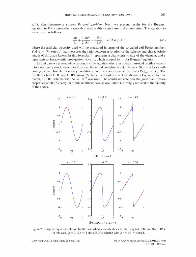
4.1.1. One-dimensional viscous Burgers’ problem. Next, we present results for the Burgers’equation in 1D in cases where smooth initial conditions give rise to discontinuities. The equation tosolve reads as follows:

@u

@tC1

2

@u2

@xD �

@2u

@x2, in � 2 Œ0, 1�, (45)

where the artificial viscosity used will be measured in terms of the so-called cell Peclet number:Pejcell D .h=p/.c=�/ that measures the ratio between resolution of the scheme and characteristiclength of diffusion layers. In this formula, h represents a characteristic size of the element, and crepresents a characteristic propagation velocity, which is equal to juj for Burgers’ equation.

The first case we presented corresponds to the situation where an initial sinusoidal profile steepensinto a stationary shock wave. For this case, the initial condition is set to be u.x, 0/D sin.2x/ withhomogeneous Dirichlet boundary conditions, and the viscosity is set to zero (Pejcell D 1). Theresults for both HDG and HDPG using 25 elements of order p D 3 are shown in Figure 2. To timemarch, a BDF3 scheme with �t D 10�2 was used. The results indicate how the good stabilizationproperties of HDPG carry on to this nonlinear case as oscillation is strongly reduced in the vicinityof the shock.

0 0.5 1−1.5

−1

−0.5

0

0.5

1

1.5

Solu

tion

0 0.5 1−1.5

−1

−0.5

0

0.5

1

1.5

0 0.5 1−1.5

−1

−0.5

0

0.5

1

1.5

(a) HDG, = 3

0 0.5 1−1.5

−1

−0.5

0

0.5

1

1.5

Solu

tion

0 0.5 1−1.5

−1

−0.5

0

0.5

1

1.5

0 0.5 1−1.5

−1

−0.5

0

0.5

1

1.5

(b) HDPG, = 3, = 4

Figure 2. Burgers’ equation solution for the case where a steady shock forms using (a) HDG and (b) HDPG.In this case, p D 3, �p D 4 and a BDF3 scheme with �t D 10�2 is used.



To further confirm this, we apply HDPG to the same equation with an initial condition consistingof a smoothed version of the hat function

u.x, 0/D

²1 if x 2 Œ0.2, 0.5�0 otherwise,

(46)

and homogeneous Dirichlet boundary conditions. This setting generates both a moving shock andan expansion fan that is integrated in time using a BDF3 scheme with �t D 10�2. For this case,25 elements of order p D 3 are used, combined with constant viscosity � such that Pejcell D 10.The results, included in Figure 3, show the evolution of the shock and fan when HDG and HDPGare used. As we can see, while both schemes propagate the shock at the right speed, thanks to beingconservative, the HDPG solution is significantly less oscillatory.

0 0.5 1

0

0.5

1

Solu

tion

0 0.5 1

0

0.5

1

0 0.5 1

0

0.5

1

0 0.5 1

0

0.5

1

0 0.5 1

0

0.5

1

0 0.5 1

0

0.5

1

(a) HDG, = 3

0 0.5 1

0

0.5

1

Solu

tion

0 0.5 1

0

0.5

1

0 0.5 1

0

0.5

1

0 0.5 1

0

0.5

1

0 0.5 1

0

0.5

1

0 0.5 1

0

0.5

1

(b) HDPG, = 3 , = 4

Figure 3. Burgers’ equation solution for the case where a moving shock and an expansion fan form using(a) HDG and (b) HDPG. In this case, p D 3, �p D 4 and a BDF3 scheme with �t D 10�2 is used.



4.2. Peterson’s example

The Peterson’s example [32] is a famous test case in which DG methods are known to yield pC1=2order of convergence. The DPG method proposed in [7,31] is the first of them that produces optimalconvergence of order pC 1. The problem to solve reads as follows:

r � .cu/D 0, in � 2 Œ0, 1�� Œ0, 1�, (47)

where c D .0, 1/ and the boundary conditions are Dirichlet on the sides and bottom u.x,y/ D u0,and free outflow on the top. In this case, both u0.x/ D x2 and u0.x/ D sin.6x/ have been used asboundary condition, following Peterson [32] and Demkowicz et al. [31], respectively.

The results for the error and the convergence rate of the HDPG scheme, in this case, aresummarized in Table I. Here, h is an indicator of the element size. As we can see, the expectedp C 1=2 convergence rate for HDG is achieved, while HDPG approaches p C 1 for �p > 3.This shows the enhanced stability of the proposed scheme. Notice for �p D 1, the error of theHDPG scheme did not converge, even though the solver did not report conditioning issues with thematrices involved. The analysis carried out in [37] for the original DPG scheme partially explainsthis behavior.

4.2.1. Two-dimensional viscous Burgers’ equation. In the last example, we apply the HDPGscheme to solve a two-dimensional Burgers’ equation:

1

2

@.u2/

@xC@u

@yD �

�@2u

@x2C@2u

@y2

�, in � 2 Œ0, 1�� Œ0, 1�. (48)

Here, the boundary conditions need to be consistent with the hyperbolic character of the equation.In particular, we will set u.x,y/D 1� 2x on the x D 0, x D 1 and y D 0 sides of the domain andextrapolation boundary conditions at y D 1.

The results in Figure 4 compare HDG and HDPG for the case of a regular mesh of 98 triangularelements, using p D 4 and no viscosity (Pejcell D 1). As we can see, the HDPG solution issignificantly less oscillatory with an enriched space of only order �p D 2 higher.

These results might be influenced by the regularity of the mesh. In order to assess the method, weperformed the computation of similar cases on an unstructured mesh. It is worth to mention that for

Table I. Error and convergence rate for Peterson’s example using hybridizable discontinuous Galerkin(HDG) and hybridized discontinuous Petrov–Galerkin (HDPG) with p D 1.

(a) u0 D x2 (b) u0 D sin.6x/

Method �p h ku� uhk2 Order Method �p h ku� uhk2 Order

HDG � 0.167 3.19� 10�3 � HDG � 0.167 3.77� 10�2 �

HDG � 0.083 1.18� 10�3 1.44 HDG � 0.083 1.49� 10�2 1.33HDG � 0.042 4.04� 10�4 1.54 HDG � 0.042 5.24� 10�3 1.51HDG � 0.021 1.56� 10�4 1.37 HDG � 0.021 2.04� 10�3 1.37HDG � 0.010 5.36� 10�5 1.54 HDG � 0.010 6.95� 10�4 1.55

HDPG 2 0.167 2.92� 10�3 � HDPG 2 0.167 3.53� 10�2 �

HDPG 2 0.083 1.08� 10�3 1.43 HDPG 2 0.083 1.37� 10�2 1.37HDPG 2 0.042 3.14� 10�4 1.78 HDPG 2 0.042 4.08� 10�3 1.74HDPG 2 0.021 1.24� 10�4 1.35 HDPG 2 0.021 1.61� 10�3 1.34HDPG 2 0.010 4.55� 10�5 1.44 HDPG 2 0.010 5.91� 10�4 1.44

HDPG 3 0.167 2.10� 10�3 � HDPG 3 0.167 2.71� 10�2 �

HDPG 3 0.083 5.90� 10�4 1.83 HDPG 3 0.083 7.51� 10�3 1.85HDPG 3 0.042 1.59� 10�4 1.90 HDPG 3 0.042 2.01� 10�3 1.90HDPG 3 0.021 4.16� 10�5 1.93 HDPG 3 0.021 5.32� 10�4 1.92HDPG 3 0.010 1.11� 10�5 1.91 HDPG 3 0.010 1.43� 10�4 1.90



Figure 4. Solution to the Burgers equation in 2D using both (a) HDG and (b) HDPG on a structured mesh.Notice the reduced oscillation that HDPG introduces compared to HDG at the shock location.

Table II. Comparison of maximum relative oscillation (%) at theshock as a function of viscosity between HDG and HDPG for thespace–time Burgers’ equation using p D 4 and �p D 2 on an

unstructured grid.

Pejcel l HDG oscillation (%) HDPG oscillation (%)

2 0 010 44 3050 90 42100 110 431000 � 441 � 44

Figure 5. Solution to the Burgers equation in 2D using both (a) HDG and (b) HDPG on an unstructuredmesh. Notice the oscillation present in the HDG solution around the elements that contain the discontinuity,that is not present in the HDPG solution. Notice also the slight bending of the shock because of the mesh inthe HDPG case, which indicates that the stabilization mechanism depends on the geometry of the element.

the case without viscosity, the HDG scheme failed to deliver a solution. In particular, divergence ofthe simulation occurred owing to the extreme oscillation around the discontinuity. To explore thisphenomenon, different values of Pejcell 2 Œ2,1/ were used to add extra stability to the scheme.



This revealed that the HDPG scheme converged in all cases whereas the HDG scheme did not. Thedifferent overshoot present at the shock for both schemes, as a function of the artificial viscosity, issummarized in Table II. As we can see, once the viscous effects are small enough, the oscillation ofthe HDPG solution no longer grows, indicating that the stabilization mechanism introduced by theoptimal test function is suitable for under-resolved situations. A visual comparison of the solutionis included in Figure 5.

5. CONCLUSIONS

In this paper, we have presented the HDPG approach for scalar conservation laws. Our objectivewas to devise a method with the same complexity as the original HDG scheme, but with enhancedstability in the presence of discontinuities. To do so, the HDG scheme was combined with thetheory of the optimal test functions, suitably modified to account for nonlinearity and to enforceconservation.

The scheme has been applied to linear convection and Burgers’ equation in 1D and 2D, withand without the addition of artificial viscosity, and compared to the HDG scheme. The resultsindicate that HDPG delivers less oscillatory solutions in the presence of discontinuities, becauseof the stabilization role of the optimal test functions. In particular, optimal p C 1 error estimateshave been experimentally confirmed for the pC 1=2 sub-optimal case constructed by Peterson.

We end the paper by noting that the application of HDPG to systems of conservation laws suchas the Euler or Navier–Stokes equations is a subject of current research.

APPENDIX A: RESIDUAL AND DERIVATIVES EVALUATION

In this appendix, we will describe the different terms that enter the HDPG formulation. In whatfollows, the unknown Z that was introduced to alleviate the notation, will be split in the originalcomponents u and Q. Let �i denote the i th basis function of the space Pp.K/, of dimension m.Similarly, let i denote the i th basis function of the space PpC�p.K/, of dimension n. Let u 2Rm

and Q 2 Rm�d represent the vector of coefficients of the expansion of uh and qh in the basis forPp.K/ and .Pk.K//d , respectively.

uh D

mXiD1

ui�i , qhj D

mXiD1

qij�i j D 1, : : : , d .

Also, let �ij denote the i th basis function for the space Pp.EK/ at the j th local face. This spacehas dimension t at each face and can be broken in f face contributions. We denote by OU 2 Rt�f

the vector of coefficients of the expansion of Ouh in the basis �ij .

Ouh D

tXiD1

fXjD1

OUij �ij .

We obtain the residuals of the local problem by integration against each element of the test space;

rKui D� uh�t

, i�KC hF. Ouh/ � nC �qh � nC �.uh, Ouh/.uh � Ouh/, i i@K

� .F.uh/� �qh,r i /K �

f C

us�1h

�t, i

!K

, i D 1, : : : ,n,

rKqij D .qhj ,�i /K C

�uh,

@�i

@xj

�K

� h Ouh,�i � nj i@K , i D 1, : : : ,m j D 1, : : : , d ,

XV ik D . j , j /K , i D 1, : : : ,n k D 1, : : : ,n,

where, following the HDPG scheme presented earlier, the residual for the conservation law (ruK) isintegrated against polynomials of order �p higher (n > m).



With this in mind, we can compute the different Jacobians and second derivatives required in thelocal iteration as follows:

@rKui@ukD

��k

�t, i

�K

C h@�.uh, Ouh/

@uh�k.uh � Ouh/, i i@K C h�.uh, Ouh/�k , i i@K

�

�@F.uh/@uh

�k ,r i

�K

, i D 1, : : : ,n k D 1, : : : ,m,

@rKui@qkl

D h��k � nl , i i@K , i D 1, : : : ,n k D 1, : : : ,m l D 1, : : : , d ,

@rKqij

@ukD

��k ,

@�i

@xj

�K

, i D 1, : : : ,m j D 1, : : : , d k D 1, : : : ,m,

@rKqij

@qklD .ıjk�k ,�i /K , i D 1, : : : ,m j D 1, : : : , d k D 1, : : : ,m l D 1, : : : , d ,

@2rKui@uk@ur

D h@2�.uh, Ouh/

@u2h

�k�r.uh � Ouh/, i i@K C h2@�.uh, Ouh/

@uh�k�r , i i@K

�

@2F.u2

h/

@uh�k�r ,r i

!K

, i D 1, : : : ,n k D 1, : : : ,m r D 1, : : : ,m,

where only non-zero second derivatives have been computed.Similarly, we can compute the terms required for the sensitivities as follows:

@rKui@Ukl

D h@F. Ouh/ � n@ Ouh

�kl , i i@K C h@�.uh, Ouh/

@ Ouh�kl .uh � Ouh/, i i@K�

h�.uh, Ouh/�kl , i i@K , i D 1, : : : ,n k D 1, : : : , t l D 1, : : : ,f ,

@rKqij

@UklD�h�kl ,�i � nj i@K , i D 1, : : : ,m j D 1, : : : , d k D 1, : : : , t l D 1, : : : ,f ,

@2rKui@ur@Ukl

D h@2�.uh, Ouh/

@ Ouh@uh�kl�r.uh � Ouh/, i i@K C h

�@�.uh, Ouh/

@ Ouh�@�.uh, Ouh/

@uh

��r�kl , i i@K ,

i D 1, : : : ,m j D 1, : : : , d k D 1, : : : , t l D 1, : : : ,f , r D 1, : : : ,m,

again, only the non-zero terms have been computed.Finally, we need to derive expressions for the computation of the global problem r Ou D 0 and its

derivatives. Following the usual finite element procedure, we introduce an index mapping from theDOFs of the faces, OUij , to the global DOFs of the space Mp

h, denoted by .i , j , k/. The residual

can then be computed by summation over all the elements as follows:

r Ou�.i ,j ,k/D

eXkD1

hF. Ouh/ � nC �qh � nC �.uh, Ouh/.uh � Ouh/, �ij iKk

Similarly, we can compute the derivatives that enter (33):

@r Ou�.i ,j ,k/

@ Ou�.r ,s,k/D

eXkD1

h

�@F. Ouh/ � n@ Ouh

C@�.uh, Ouh/

@ Ouh.uh � Ouh/� �.uh, Ouh/

��rs , �ij iKk

C

eXkD1

h��k � nl@Qkl

@ OUrs, �ij iKk

C

eXkD1

h

�@�.uh, Ouh/

@uh.uh � Ouh/C �.uh, Ouh/

�@uk

@ OUrs�k , �ij iKk .



ACKNOWLEDGEMENTS

D. Moro would like to acknowledge the CajaMadrid Foundation for the Graduate Studies Scholarship thatfunded his work. N.C. Nguyen and J. Peraire gratefully acknowledge the support provided by the SingaporeMIT Alliance as well as the Air Force Office of Scientific Research under the MURI program on biologicallyinspired flight. The authors would like to acknowledge Prof. J. Gopalakrishnan for his useful suggestionsand comments and Dr. X. Roca for his comments and the mesh used for the 2D cases.

REFERENCES

1. Arnold D, Brezzi F, Cockburn B, Marini L. Unified analysis of discontinuous Galerkin methods for elliptic problems.SIAM Journal on Numerical Analysis 2002; 39(5):1749–1779.

2. Barter G, Darmofal D. Shock capturing with PDE-based artificial viscosity for DGFEM: part I. Formulation. Journalof Computational Physics 2010; 229(5):1810–1827.

3. Bassi F, Rebay S. A high-order accurate discontinuous finite element method for the numerical solution of thecompressible Navier–Stokes equations. Journal of Computational Physics 1997; 131(2):267–279.

4. Baumann C, Oden J. A discontinuous HP finite element method for convection–diffusion problems. ComputerMethods in Applied Mechanical Engineering 1999; 175(3-4):311–341.

5. Cockburn B, Shu C. The local discontinuous Galerkin method for time-dependent convection–diffusion systems.SIAM Journal on Numerical Analysis 1998; 35(6):2440–2463.

6. Cockburn B, Shu C. Runge–Kutta discontinuous Galerkin methods for convection-dominated problems. Journal ofScientific Computing 2001; 16(3):173–261.

7. Demkowicz L, Gopalakrishnan J. A class of discontinuous Petrov-Galerkin methods. Part I: the transport equation.Computer Methods in Applied Mechanical Engineering 2010; 199(23-24):1558–1572.

8. Hartmann R, Houston P. Adaptive discontinuous Galerkin finite element methods for the compressible Eulerequations. Journal of Computational Physics 2002; 183(2):508–532.

9. Hesthaven J, Warburton T. Nodal high-order methods on unstructured grids: I. Time-domain solution of Maxwell’sequations. Journal of Computational Physics 2002; 181(1):186–221.

10. Klaij C, Van der Vegt J, Van der Ven H. Space–time discontinuous Galerkin method for the compressibleNavier–Stokes equations. Journal of Computational Physics 2006; 217(2):589–611.

11. Lomtev I, Karniadakis G. A discontinuous Galerkin method for the Navier–Stokes equations. International Journalfor Numerical Methods in Engineering 1999; 29(5):587–603.

12. Peraire J, Persson PO. The compact discontinuous Galerkin (CDG) method for elliptic problems. SIAM Journal onScientific Computing 2008; 30(4):1806–1824.

13. Reed N, Hill T. Triangle mesh methods for the neutron transport equation. Technical Report LA2 UR-73-479,Los Alamos Scientific Laboratory, 1973.

14. Cockburn B, Gopalakrishnan J, Lazarov R. Unified hybridization of discontinuous Galerkin, mixed and continuousGalerkin methods for second order elliptic problems. SIAM Journal on Numerical Analysis 2009; 47(2):1319–1365.

15. Nguyen NC, Peraire J, Cockburn B. An implicit high-order hybridizable discontinuous Galerkin method for linearconvection–diffusion equations. Journal of Computational Physics 2009; 228(9):3232–3254.

16. Nguyen NC, Peraire J, Cockburn B. An implicit high-order hybridizable discontinuous Galerkin method for nonlinearconvection–diffusion equations. Journal of Computational Physics 2009; 228(23):8841–8855.

17. Nguyen NC, Peraire J, Cockburn B. High-order implicit hybridizable discontinuous Galerkin methods for acousticsand elastodynamics. Journal of Computational Physics 2011; 230(10):3695–3718.

18. Soon SC, Cockburn B, Stolarski HK. A hybridizable discontinuous Galerkin method for linear elasticity.International Journal for Numerical Methods in Engineering 2009; 80(8):1058–1092.

19. Cockburn B, Gopalakrishnan J. The derivation of hybridizable discontinuous Galerkin methods for Stokes flow.SIAM Journal on Numerical Analysis 2009; 47:1092–1125.

20. Cockburn B, Gopalakrishnan J, Nguyen NC, Peraire J, Sayas F. Analysis of HDG methods for Stokes flow.Mathematics of Computation 2011; 80:723–760.

21. Nguyen NC, Peraire J, Cockburn B. A hybridizable discontinuous Galerkin method for Stokes flow. ComputerMethods in Applied Mechanical Engineering 2010; 199(9-12):582–597.

22. Nguyen NC, Peraire J, Cockburn B. An implicit high-order hybridizable discontinuous Galerkin method for theincompressible Navier–Stokes equations. Journal of Computational Physics 2011; 230(4):1147–1170.

23. Nguyen NC, Peraire J, Cockburn B. A hybridizable discontinuous Galerkin method for the incompressible Navier–Stokes equations (AIAA Paper 2010-362). Proceedings of the 48th AIAA Aerospace Sciences Meeting and Exhibit,Orlando, Florida, January 2010.

24. Nguyen NC, Peraire J, Cockburn B. Hybridizable discontinuous Galerkin methods. In Lecture Notes in Computa-tional Science and Engineering, Vol. 76. Springer: Berlin, 2011; 63–84.

25. Nguyen NC, Peraire J, Cockburn B. A comparison of HDG methods for Stokes flow. Journal of Scientific Computing2010; 45:215–237.

26. Peraire J, Nguyen NC, Cockburn B. A hybridizable discontinuous Galerkin method for the compressible Euler andNavier–Stokes equations (AIAA Paper 2010-363). Proceedings of the 48th AIAA Aerospace Sciences Meeting andExhibit, Orlando, FL, USA, 2010.



27. Nguyen NC, Peraire J, Cockburn B. Hybridizable discontinuous Galerkin methods for the time-harmonic Maxwell’sequations. Journal of Computational Physics 2011; 230(19):7151–7175.

28. Güzey S, Cockburn B, Stolarski HK. The embedded discontinuous Galerkin method: application to linear shellproblems. International Journal for Numerical Methods in Engineering 2007; 70(7):757–790.

29. Peraire J, Nguyen NC, Cockburn B. An embedded discontinuous Galerkin method for the compressible Euler andNavier–Stokes equations. Proceedings of the 20th AIAA Computational Fluid Dynamics Conference, Honolulu,Hawaii, 2011.

30. Cockburn B, Dong B, Guzmán J, Restelli M, Sacco R. A hybridizable discontinuous Galerkin method for steady-stateconvection–diffusion-reaction problems. SIAM Journal on Scientific Computing 2009; 31(5):3827–3846.

31. Demkowicz L, Gopalakrishnan J. A class of discontinuous Petrov–Galerkin methods. Part II: optimal test functions.Numerical Methods for Partial Differential Equations 2010; 27(1):70–105.

32. Peterson TE. A note on the convergence of the discontinuous Galerkin method for a scalar hyperbolic equation. SIAMJournal on Numerical Analysis 1991; 28(1):133–140.

33. Demkowicz L, Gopalakrishnan J, Niemi A. A class of discontinuous Petrov–Galerkin methods. Part III: adaptivity.Technical Report 10-1, ICES, 2010.

34. Babuška I. Error-bounds for finite element method. Numerische Mathematik 1971; 16(4):322–333.35. Bottasso C, Micheletti S, Sacco R. A multiscale formulation of the discontinuous Petrov–Galerkin method for

advective–diffusive problems. Computer Methods in Applied Mechanical Engineering 2005; 194(25-26):2819–2838.36. Chan J, Demkowicz L, Moser R, Roberts N. A class of discontinuous Petrov–Galerkin methods. Part V: solution of

1D Burgers and Navier–Stokes Equations. Technical Report 10-25, ICES, 2010.37. Gopalakrishnan J, Qiu W. An analysis of the practical DPG method, 07 2011. http://arxiv.org/abs/1107.4293v1.


a hybridized discontinuous petrov–galerkin scheme for scalar...

Documents