Transportation Research Part C 37 (2013) 223–237

Contents lists available at SciVerse ScienceDirect

Transportation Research Part C

journal homepage: www.elsevier .com/locate / t rc

A hybrid multi-scale approach for simulation of pedestriandynamics

0968-090X/$ - see front matter � 2013 Elsevier Ltd. All rights reserved.http://dx.doi.org/10.1016/j.trc.2013.03.005

⇑ Corresponding author. Tel.: +49 8928925117.E-mail addresses: kneidl@tum.de (A. Kneidl), hartmann.dirk@siemens.com (D. Hartmann), andre.borrmann@tum.de (A. Borrmann).

A. Kneidl a, D. Hartmann b, A. Borrmann a,⇑a Technische Universität München, 80290 München, Germanyb Siemens Corporate Technology, 80200 München, Germany

a r t i c l e i n f o

Article history:Received 21 August 2012Received in revised form 15 March 2013Accepted 17 March 2013

Keywords:Pedestrian dynamicsNavigationFloor fieldHybrid modelNavigation graphRoute choiceMicroscopic model

a b s t r a c t

One of the most important aspects for a realistic prediction of pedestrian flows is the mod-elling of human navigation in normal situations such as early design phases of buildings ortransportation systems and hubs as well as in evacuation studies to enhance safety inexisting infrastructures. To overcome the limitations of current navigation models, thispaper proposes a new hybrid multi-scale model, which closely links information betweenthe small-scale and large-scale navigation layer to improve the navigational behaviour. Inthe presented hybrid navigation model, graph-based methods using visibility graphs areused to model large-scale wayfinding decisions. The pedestrians’ movements betweentwo nodes of the navigation graph are modelled by means of a dynamic navigation field.The navigation field is updated dynamically during the runtime of the simulation, explicitlyconsidering other pedestrians for determining the fastest path.

The proposed hybrid approach provides a realistic modelling of human navigationalbehaviour and thus a realistic prediction of flows since it reflects the human cognitive pro-cesses triggered by wayfinding tasks. This includes taking into account other pedestriansfor routing decisions who are visible from the current position of the considered pedes-trian. The paper discusses the concept and the technical details of the proposed hybridmulti-scale approach in detail and presents an extensive case study demonstrating itsadvantages.

� 2013 Elsevier Ltd. All rights reserved.

1. Introduction

Studying emerging phenomena in pedestrian crowds is a classical subject in complexity science. Due to an improvementof algorithms as well as computational power, the simulation of pedestrian dynamics has attracted many researchers in thefields of safety and transportation science. On the one hand, pedestrian flow simulations are used for virtual evacuation stud-ies (e.g. Lämmel et al., 2010; Klüpfel et al., 2004; Rodriguez and Amato, 2010; Teknomo and Fernandez, 2012; Guo et al.,2011) and the proposal of corresponding optimal strategies (Hamacher and Tjandra, 2002) to enhance the safety of eventsand buildings.

On the other hand, simulation of pedestrian flows is an emerging topic in the early design phase of public transport sys-tems, public transport hubs (Pelechano and Malkawi, 2008; Zhang et al., 2008) such as stations (Ding et al., 2011) or evenlarge infrastructures and urban areas (e.g. Loscos et al., 2003; Haklay et al., 2001) as well as their safety (Shi et al., 2012)and operation (Rindsfüser et al., 2007). Of course, the utility of such virtual approaches depends crucially on the realismas well as on the computational speed of virtual approaches (Pelechano and Malkawi, 2008). If the realism of simulations

224 A. Kneidl et al. / Transportation Research Part C 37 (2013) 223–237

is not sufficiently accurate, e.g. appearance of unnatural congestions, prediction of the simulations would yield improper de-signs. At the same time, if computations take too long, virtual approaches can hardly be used for design studies and designoptimisation.

From a conceptual point of view, models of pedestrian flows can be divided into microscopic models, simulating thebehaviour of single pedestrians and their interaction, and macroscopic models, considering flows of pedestrian entities. Thus,being interested in local small-scale behaviour of pedestrian flows, microscopic models are the approach of choice. They canbe distinguished into force models (e.g. Burstedde et al., 2001; Klüpfel, 2003; Kretz and Schreckenberg, 2006; Chraibi et al.,2011a), discrete-choice models (e.g. Antonini et al., 2006; Robin et al., 2009; Hoogendoorn and Bovy, 2004; Guo and Huang,2012) or agent-based models (e.g. Rindsfüser et al., 2007; Dijkstra et al., 2006; Ronald et al., 2007).

To study large-scale behaviour and large scale navigation, macroscopic models are typically preferred like network-basedmodels (e.g. Hamacher and Tjandra, 2002; Mitchell and MacGregor Smith, 2001) or fluid dynamics models (e.g. Henderson,1974; Helbing, 1992). Very often one is interested in local phenomena, e.g. the evolution of congestions, which are inducedby large scale navigation, e.g. many people are choosing the same route.

This challenge, bridging the gap between small-scale and large-scale aspects can be resolved using multi-scale models,e.g. combining graph-based approaches either with force models (e.g. Wagoum et al., 2012; Kretz et al., 2011) or with agenttype models (e.g. Funge et al., 1999; Reynolds, 1999; Rindsfüser et al., 2007; Lerner et al., 2007; Sud et al., 2008; Teknomo,2008; Asano et al., 2010; Dijkstra et al., 2006; Ronald et al., 2007).

However, these multi-scale models typically combine microscopic and macroscopic models in a very simplistic fashion.Thus the limitations of small-scale (e.g. being short-sighted) and large scale (e.g. not considering other moving pedestriansfor route choice decisions) are usually not resolved. Information between the layers is not exchanged from the microscopiclayer to the macroscopic layer and vice versa. Typically, the macroscopic layer provides the next intermediate destination topedestrians steering in the microscopic layer and no information sharing between the microscopic and the macroscopic layertakes place.

The focus of the paper is the combination of advanced microscopic navigation strategies with macroscopic navigationstrategies. Both state-of-the-art concepts alone including their qualitative properties, especially their realism with respectto real world scenarios, have been studied extensively in the literature. Combining both concepts, the realistic qualitativeproperties are inherited but the drawbacks of microscopic navigation concepts (extensive computation times) and macro-scopic navigation strategies (difficulty to estimate travel times) are resolved.

We propose a new holistic multi-scale model unifying the advantages of the single layers and overcoming their limita-tions. Information is shared between the layers, such that the above mentioned issues are resolved. At the same time theapproach allows an efficient realisation from a computational point of view. We demonstrate this new approach by extend-ing a well established cellular automaton model (Köster et al., 2010). However, the concepts can be easily generalised toother microscopic pedestrian simulators. Due to computational efficiency as well as its high degree of realism, we believethat the developed concepts provide a valuable tool for optimising transportation systems, buildings, as well as large infra-structures such as transportation hubs or even urban areas.

This article is structured as follows: First, we review existing multi-scale models in Section 2 and outline their limitations.Section 3 describes in detail the construction and implementation of each layer. In Section 4 the combination of these layersis explained. To show the improvements in the simulation results, various tests have been conducted and are presented inSection 5. A discussion concludes the article.

2. State of the art and limitations of multi-scale models

Multi-scale models typically consist of two layers: a small-scale layer modelling the navigation of pedestrians to a des-ignated destination and a large-scale layer modelling strategic navigation, i.e. choosing different (intermediate) destinations.

On the small-scale layer, pedestrians are steered to a designated destination by forces similar to Newtonian particlemechanics. Typically, these forces are modelled using an attractive force or potential-based approach. Assuming a conserva-tive force, i.e. the local force is given by the gradient of the potential, both approaches basically coincide. Continuous socialforce models (e.g. Helbing and Molnár, 1995; Lakoba et al., 2005; Löhner, 2010; Parisi et al., 2009; Chraibi et al., 2010; Chraibiet al., 2011b; Yu et al., 2005) typically use a force-based description whereas cellular automata, i.e. space-discretized models,typically rely on a potential-based description.

In the following, we will restrict ourselves to a potential-based cellular automaton model (Köster et al., 2010), which canbe always interpreted in a force-based description assuming that forces are given by the gradients of the correspondingpotentials. In the potential-based approach, a pedestrian’s movement towards the destination is realised by a decreasing po-tential value towards the direction of the destination. Obstacles and other pedestrians walking in the vicinity of the pedes-trian are considered via a repulsion force or repulsion potential (e.g. Kretz and Schreckenberg, 2006; Chraibi et al., 2011a;Köster et al., 2010) and thus added to the potential value. Typically, it is assumed that single pedestrians have a repellingpotential of a certain width, which might also have a certain spatial structure depending on the direction of movement(Klüpfel, 2003; Köster et al., 2010). Using a cellular automaton, these pedestrians can be detected very easily in the nearbysurrounding by simply checking neighbouring cells. The potential-based steering behaviour is often referred to as floor fieldor navigation field based behaviour and a variety of approaches to construct corresponding potential fields have been pro-

A. Kneidl et al. / Transportation Research Part C 37 (2013) 223–237 225

posed (e.g. Schadschneider et al., 2009; Burstedde et al., 2001; Blue and Adler, 2001; Klüpfel, 2003; Köster et al., 2010; Nish-inari et al., 2004; Kretz, 2009; Varas et al., 2007; Yamamoto et al., 2007; Guo et al., 2011).

To model the large-scale behaviour, i.e. the navigation strategy of pedestrians, graph-based approaches are used inmost multi-scale models (e.g. Gloor et al., 2004; Gunnar, 1998; Teknomo and Millonig, 2007; Kirik et al., 2009; Höckeret al., 2010). Based on a given geometry, possible routes are identified and from these a graph is constructed. Accordingto given preferences, pedestrians move through the graph from their origin to their final destination via intermediatedestinations as given by the vertices of the graph. Such intermediate destinations could be crossings or landmarks. Thedecision of which way to take at each intermediate destination might depend on environmental conditions, e.g. choos-ing illuminated paths in the evening, and can vary from pedestrian to pedestrian, e.g. take the shortest path, take thefastest path, avoid congestions, follow signage, follow friends, etc. as discussed in Pelechano and Malkawi (2008) orGolledge (1999). The different strategies are typically modelled by different routing algorithms. These reflect differentbehaviours by determining the best paths with respect to certain criteria, i.e. certain metrics or edge weights. However,most of the algorithms use travelling times as edge weights, which are often approximated by heuristics or meanvalues.

So far, these two layers have been combined to form a multi-scale model as follows: The navigation graph is used to gen-erate pedestrians’ paths based on a specific navigation strategy. Paths themselves consist of a list of intermediate destina-tions. The navigation field is then used to navigate pedestrians between these intermediate destinations until the finaldestination is reached. Although the combination of the layers already improves the realism of simulations, since small-scaleaspects (e.g. avoiding other moving pedestrians in a close vicinity) and large scale aspects (e.g. navigation strategy) are ad-dressed, there are still several open issues to be resolved:

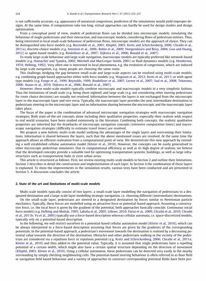
On the small-scale layer, typically only static floor fields are considered (e.g. Burstedde et al., 2001; Blue and Adler, 2001;Klüpfel, 2003; Köster et al., 2010; Nishinari et al., 2004; Kretz, 2009; Varas et al., 2007; Yamamoto et al., 2007), i.e. floor fieldsdetermined in the initialization phase of the simulation. Other pedestrians who are not in close vicinity, e.g. large conges-tions, are not taken into account. Thus, such static navigation behaviour often leads to unrealistic simulation results: Pedes-trians steer towards the congestions very closely until they ‘‘see’’ the congestion. In reality, pedestrians are able to see acongestion earlier if it is located in their field of vision. Only recently two approaches have been proposed independentlyto include dynamic aspects (Kretz, 2009; Hartmann, 2010). This however requires a continuous update of the navigationfields, which is computationally expensive, particularly for large domains. Besides, using these dynamic floor fields, pedes-trians consider congestions, which are not visible from their actual position while making their navigation decisions. Anexample is given in Fig. 1.

On the large-scale, routes that are based on heuristic edge weights are typically determined, in most cases heuristic esti-mates of travelling times. These are usually estimated by the number of pedestrians moving along an edge (i.e. edge densi-ties, e.g. Kirik.2009). However, since densities are local properties (e.g. congestions) and are not constant on the whole edgearea, these estimates are not sufficiently exact. Consider for example a long edge, where a small congestion occurs at the veryend (c.f. Fig. 5). This edge would not been chosen due to the longer travel time derived from the slow velocity within thecongested area, although the congestion would vanish until a pedestrian reaches this location.

3. Ingredients of a holistic multi-scale model

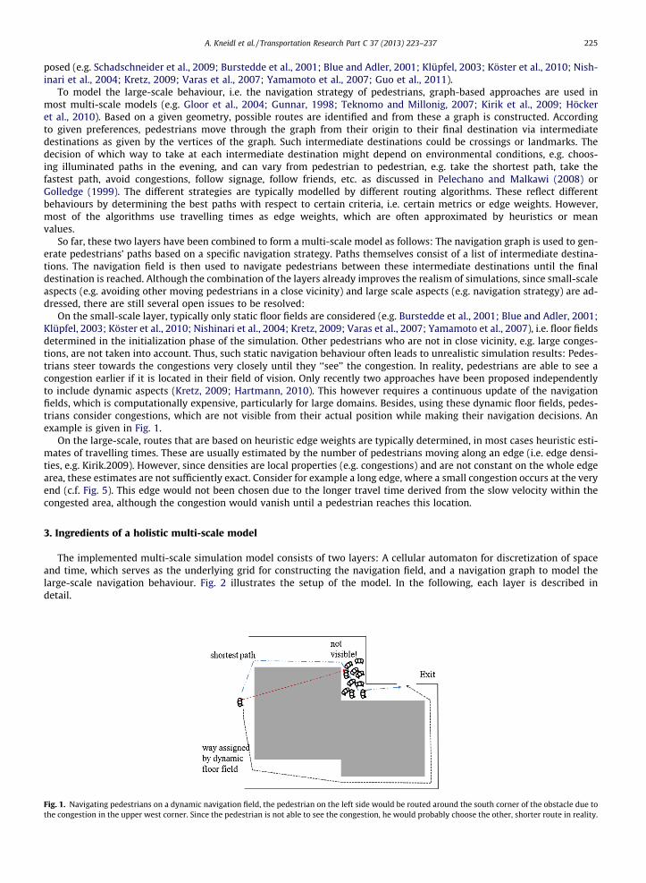
The implemented multi-scale simulation model consists of two layers: A cellular automaton for discretization of spaceand time, which serves as the underlying grid for constructing the navigation field, and a navigation graph to model thelarge-scale navigation behaviour. Fig. 2 illustrates the setup of the model. In the following, each layer is described indetail.

Fig. 1. Navigating pedestrians on a dynamic navigation field, the pedestrian on the left side would be routed around the south corner of the obstacle due tothe congestion in the upper west corner. Since the pedestrian is not able to see the congestion, he would probably choose the other, shorter route in reality.

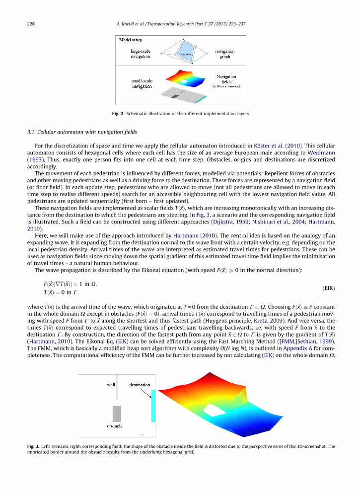
Fig. 2. Schematic illustration of the different implementation layers.

226 A. Kneidl et al. / Transportation Research Part C 37 (2013) 223–237

3.1. Cellular automaton with navigation fields

For the discretization of space and time we apply the cellular automaton introduced in Köster et al. (2010). This cellularautomaton consists of hexagonal cells where each cell has the size of an average European male according to Weidmann(1993). Thus, exactly one person fits into one cell at each time step. Obstacles, origins and destinations are discretizedaccordingly.

The movement of each pedestrian is influenced by different forces, modelled via potentials: Repellent forces of obstaclesand other moving pedestrians as well as a driving force to the destination. These forces are represented by a navigation field(or floor field). In each update step, pedestrians who are allowed to move (not all pedestrians are allowed to move in eachtime step to realise different speeds) search for an accessible neighbouring cell with the lowest navigation field value. Allpedestrians are updated sequentially (first born – first updated).

These navigation fields are implemented as scalar fields Tð~xÞ, which are increasing monotonically with an increasing dis-tance from the destination to which the pedestrians are steering. In Fig. 3, a scenario and the corresponding navigation fieldis illustrated. Such a field can be constructed using different approaches (Dijkstra, 1959; Nishinari et al., 2004; Hartmann,2010).

Here, we will make use of the approach introduced by Hartmann (2010). The central idea is based on the analogy of anexpanding wave. It is expanding from the destination normal to the wave front with a certain velocity, e.g. depending on thelocal pedestrian density. Arrival times of the wave are interpreted as estimated travel times for pedestrians. These can beused as navigation fields since moving down the spatial gradient of this estimated travel time field implies the minimisationof travel times - a natural human behaviour.

The wave propagation is described by the Eikonal equation (with speed Fð~xÞP 0 in the normal direction):

Fig. 3.imbrica

Fð~xÞjrTð~xÞj ¼ 1 in X;

Tð~xÞ ¼ 0 in C;ðEIKÞ

where Tð~xÞ is the arrival time of the wave, which originated at T = 0 from the destination C �X. Choosing Fð~xÞ � F constantin the whole domain X except in obstacles ðFð~xÞ ¼ 0Þ, arrival times Tð~xÞ correspond to travelling times of a pedestrian mov-ing with speed F from C to~x along the shortest and thus fastest path (Huygens principle, Kretz, 2009). And vice versa, thetimes Tð~xÞ correspond to expected travelling times of pedestrians travelling backwards, i.e. with speed F from ~x to thedestination C. By construction, the direction of the fastest path from any point ~x 2 X to C is given by the gradient of Tð~xÞ(Hartmann, 2010). The Eikonal Eq. (EIK) can be solved efficiently using the Fast Marching Method ([FMM,]Sethian, 1999).The FMM, which is basically a modified heap sort algorithm with complexity O(N log N), is outlined in Appendix A for com-pleteness. The computational efficiency of the FMM can be further increased by not calculating (EIK) on the whole domain X,

Left: scenario, right: corresponding field; the shape of the obstacle inside the field is distorted due to the perspective error of the 3D-screenshot. Theted border around the obstacle results from the underlying hexagonal grid.

A. Kneidl et al. / Transportation Research Part C 37 (2013) 223–237 227

but rather stop the calculation if a corresponding navigation field has been calculated for all positions, i.e. cells, occupied bypedestrians moving to the destination C.

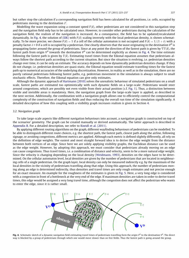
Modelling the wave expansion using a constant speed Fð~xÞ, other pedestrians are not considered in this navigation stepand the navigation field only has to be calculated once. However, to consider other pedestrians during the calculation of thenavigation field, the realism of the navigation is increased. As a consequence, the field has to be updated/recalculateddynamically. In Fig. 4, the solution of (EIK) with Fð~xÞ scaling inversely with the local pedestrian density, is shown schemat-ically. To be more precise, we choose Fð~xÞ ¼ 1 if a cell of the cellular automaton is not occupied and Fð~xÞ ¼ 1=ð1þ dÞ with apenalty factor d > 0 if a cell is occupied by a pedestrian. One clearly observes that the wave originating in the destination VD ispropagating faster around the group of pedestrians. Since at any point the direction of the fastest path is given byrTð~xÞ, thefastest path from origin VO towards the destination VD can be determined explicitly as shown in Fig. 4. The time estimatefollowing the fastest path is given by Tð~xÞ. Estimating travel times from the Eikonal equation assumes that pedestrians al-ways follow the shortest path according to the current situation. But since the situation is evolving, i.e. pedestrian densitieschange over time, it can be only an estimate. The accuracy depends on how dynamically pedestrian densities change. If theydo not change, i.e. pedestrian densities are quasi-static, the Eikonal equation would estimate travelling times for the fastestpath up to numerical accuracies of the underlying discretization. However, in reality as well as in the simulation, there are nopurely rational pedestrians following fastest paths, e.g. pedestrian movement in the simulation is always subject to smallstochastic effects. Therefore, the Eikonal equation can give only estimates.

Although the dynamic approach of Hartmann (2010) solves the unrealistic behaviour of simulated pedestrians on a smallscale, fastest paths are estimated too optimistically with such dynamic fields on a large-scale: Pedestrians would steeraround congestions, which are possibly not even visible from their actual position (c.f. Fig. 1). Thus, a distinction betweenvisible and invisible areas is mandatory. Here, the navigation graph from the large-scale layer is applied, as described inthe next section. Additionally, the combination with a navigation graph allows one to efficiently control the computationalcomplexity of the construction of navigation fields and thus reducing the overall run time of the simulation significantly. Adetailed description of how this coupling with a visibility graph increases realism is given in Section 4.

3.2. Navigation graph

To take large-scale aspects like different navigation behaviours into account, a navigation graph is constructed on top ofthe scenarios’ geometry. The graph can be created manually or derived automatically. The latter approach is described inAppendix B. For a detailed description, we refer to Kneidl et al. (2011).

By applying different routing algorithms on the graph, different wayfinding behaviours of pedestrians can be modelled. Tobe able to distinguish different route choices, e.g. the shortest path, the fastest path, closest path along the airline, followingsignage, or avoiding congestions, different metrics are applied. Although each metric is defined slightly differently, all rely onthe definition of edge weights. The easiest and most straight forward idea is to derive the edge weight from the distancebetween both vertices of an edge. Since here we are solely applying visibility graphs, the Euclidean distance can be usedas the edge weight. However, by adopting this approach, we must consider that pedestrians already moving on an edgecan cause congestions. Thus travel times, i.e. a combination of distance and velocity, seem to be a more natural edge weight.Since the velocity is changing depending on the local density (Weidmann, 1993), densities on the edges have to be deter-mined. On the cellular automaton level, local densities are given by the number of pedestrians that are located in neighbour-ing cells of a single pedestrian. On the graph layer, local density can only be measured indirectly e.g. by the maximum of thelocal densities in the vicinity of pedestrians travelling along that edge. Using this approach, the number of pedestrians mov-ing along an edge is determined indirectly, thus densities and travel times are only rough estimates and not precise enoughfor an exact measure. An example for the roughness of the estimates is given in Fig. 5. Here, a very long edge is consideredwith a congestion in front of a bottleneck at the very end of the edge. If maximum densities are taken in order to derive traveltimes, this edge would be assigned a very long travel time, although the congestion does not affect the pedestrian who wantsto enter the edge, since it is rather small.

Fig. 4. Schematic sketch of a dynamic navigation field estimating travel times of pedestrians travelling form the origin VO to the destination VD. The directway is blocked by a group of pedestrians through which one would move slower than on free fields. Thus the fastest path is going around the group.

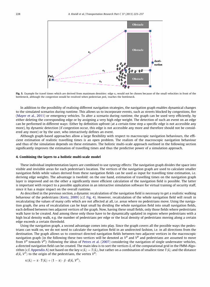
Fig. 5. Example for travel times which are derived from maximum densities: edge e2 would not be chosen because of the small velocities in front of thebottleneck, although the congestion would be resolved when pedestrian ped1 reaches the bottleneck.

228 A. Kneidl et al. / Transportation Research Part C 37 (2013) 223–237

In addition to the possibility of realising different navigation strategies, the navigation graph enables dynamical changesto the simulated scenarios during runtime. This allows us to incorporate events, such as streets blocked by congestions, fire(Mayer et al., 2011) or emergency vehicles. To alter a scenario during runtime, the graph can be used very efficiently, byeither deleting the corresponding edge or by assigning a very high edge weight. The detection of such an event on an edgecan be performed in different ways: Either by definition upfront (at a certain time step a specific edge is not accessible anymore), by dynamic detection (if congestion occur, this edge is not accessible any more and therefore should not be consid-ered any more) or by the user, who interactively defines an event.

Although graph-based approaches allow a large flexibility with respect to macroscopic navigation behaviours, the effi-cient estimation of realistic travelling times is an open problem. The realism of the macroscopic navigation behaviourand thus of the simulation depends on these estimates. The holistic multi-scale approach outlined in the following sectionsignificantly improves the estimation of travelling times and thus the predictive power of a simulation approach.

4. Combining the layers to a holistic multi-scale model

These individual implementation layers are combined to use synergy effects: The navigation graph divides the space intovisible and invisible areas for each pedestrian’s location. The vertices of the navigation graph are used to calculate smallernavigation fields while values derived from these navigation fields can be used as input for travelling time estimation, i.e.deriving edge weights. The advantage is twofold: on the one hand, estimation of travelling times on the navigation graphlayer is improved and on the other a significantly more efficient calculation of the navigation field is possible. The latteris important with respect to a possible application in an interactive simulation software for virtual training of security staff,since it has a major impact on the overall runtime.

As described in the previous section, a dynamic recalculation of the navigation field is necessary to get a realistic walkingbehaviour of the pedestrians (Kretz, 2009) (c.f. Fig. 4). However, recalculation of the whole navigation field will result inrecalculating the values of many cells which are not affected at all, i.e. areas where no pedestrians move. Using the naviga-tion graph, the area of recalculation can be kept small by dividing the whole navigation field into small navigation fields,each defined between two adjacent vertices of the graph. Now, having these small fields, only those fields where pedestrianswalk have to be created. And among these only those have to be dynamically updated in regions where pedestrians with ahigh local density walk, e.g. the number of pedestrians per edge or the local density of pedestrians moving along a certainedge exceeds a certain threshold.

Using the navigation graph, a second advantage comes into play. Since the graph covers all the possible ways the pedes-trians can walk on, we do not need to calculate the navigation field in an undirected fashion, i.e. in all directions from thedestination. The graph allows us to construct directed navigation fields between two adjacent vertices in the macroscopicnavigation graph (in the following these two vertices will be denoted as VO and VD and pedestrians are assumed to movefrom VO towards VD): Following the ideas of Petres et al. (2007) considering the navigation of single underwater vehicles,a directed navigation field can be created. The main idea is to sort the vertices~xi of the computational grid in the FMM-Algo-rithm (c.f. Appendix A) not based on the key jð~xiÞ ¼ Tð~xiÞ, but rather on a combination of smallest time Tð~xiÞ and the distancedð~xi;V

OÞ to the origin of the pedestrians, the vertex VO:

jð~xiÞ ¼ a � Tð~xiÞ þ ð1� aÞ � b � dð~xi;VOÞ;

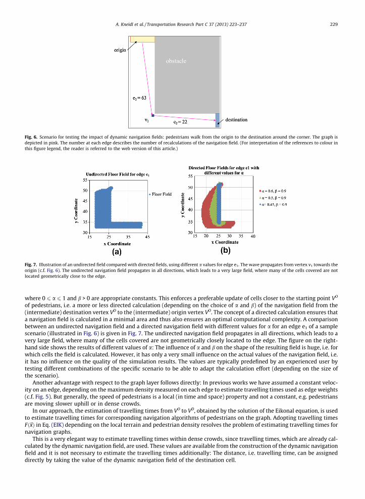
Fig. 6. Scenario for testing the impact of dynamic navigation fields: pedestrians walk from the origin to the destination around the corner. The graph isdepicted in pink. The number at each edge describes the number of recalculations of the navigation field. (For interpretation of the references to colour inthis figure legend, the reader is referred to the web version of this article.)

Fig. 7. Illustration of an undirected field compared with directed fields, using different a values for edge e1. The wave propagates from vertex v1 towards theorigin (c.f. Fig. 6). The undirected navigation field propagates in all directions, which leads to a very large field, where many of the cells covered are notlocated geometrically close to the edge.

A. Kneidl et al. / Transportation Research Part C 37 (2013) 223–237 229

where 0 6 a 6 1 and b > 0 are appropriate constants. This enforces a preferable update of cells closer to the starting point VO

of pedestrians, i.e. a more or less directed calculation (depending on the choice of a and b) of the navigation field from the(intermediate) destination vertex VD to the (intermediate) origin vertex VO. The concept of a directed calculation ensures thata navigation field is calculated in a minimal area and thus also ensures an optimal computational complexity. A comparisonbetween an undirected navigation field and a directed navigation field with different values for a for an edge e1 of a samplescenario (illustrated in Fig. 6) is given in Fig. 7. The undirected navigation field propagates in all directions, which leads to avery large field, where many of the cells covered are not geometrically closely located to the edge. The figure on the right-hand side shows the results of different values of a: The influence of a and b on the shape of the resulting field is huge, i.e. forwhich cells the field is calculated. However, it has only a very small influence on the actual values of the navigation field, i.e.it has no influence on the quality of the simulation results. The values are typically predefined by an experienced user bytesting different combinations of the specific scenario to be able to adapt the calculation effort (depending on the size ofthe scenario).

Another advantage with respect to the graph layer follows directly: In previous works we have assumed a constant veloc-ity on an edge, depending on the maximum density measured on each edge to estimate travelling times used as edge weights(c.f. Fig. 5). But generally, the speed of pedestrians is a local (in time and space) property and not a constant, e.g. pedestriansare moving slower uphill or in dense crowds.

In our approach, the estimation of travelling times from VO to VD, obtained by the solution of the Eikonal equation, is usedto estimate travelling times for corresponding navigation algorithms of pedestrians on the graph. Adopting travelling timesFð~xÞ in Eq. (EIK) depending on the local terrain and pedestrian density resolves the problem of estimating travelling times fornavigation graphs.

This is a very elegant way to estimate travelling times within dense crowds, since travelling times, which are already cal-culated by the dynamic navigation field, are used. These values are available from the construction of the dynamic navigationfield and it is not necessary to estimate the travelling times additionally: The distance, i.e. travelling time, can be assigneddirectly by taking the value of the dynamic navigation field of the destination cell.

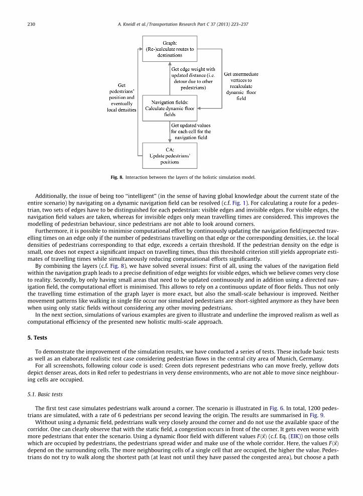
Fig. 8. Interaction between the layers of the holistic simulation model.

230 A. Kneidl et al. / Transportation Research Part C 37 (2013) 223–237

Additionally, the issue of being too ‘‘intelligent’’ (in the sense of having global knowledge about the current state of theentire scenario) by navigating on a dynamic navigation field can be resolved (c.f. Fig. 1). For calculating a route for a pedes-trian, two sets of edges have to be distinguished for each pedestrian: visible edges and invisible edges. For visible edges, thenavigation field values are taken, whereas for invisible edges only mean travelling times are considered. This improves themodelling of pedestrian behaviour, since pedestrians are not able to look around corners.

Furthermore, it is possible to minimise computational effort by continuously updating the navigation field/expected trav-elling times on an edge only if the number of pedestrians travelling on that edge or the corresponding densities, i.e. the localdensities of pedestrians corresponding to that edge, exceeds a certain threshold. If the pedestrian density on the edge issmall, one does not expect a significant impact on travelling times, thus this threshold criterion still yields appropriate esti-mates of travelling times while simultaneously reducing computational efforts significantly.

By combining the layers (c.f. Fig. 8), we have solved several issues: First of all, using the values of the navigation fieldwithin the navigation graph leads to a precise definition of edge weights for visible edges, which we believe comes very closeto reality. Secondly, by only having small areas that need to be updated continuously and in addition using a directed nav-igation field, the computational effort is minimised. This allows to rely on a continuous update of floor fields. Thus not onlythe travelling time estimation of the graph layer is more exact, but also the small-scale behaviour is improved. Neithermovement patterns like walking in single file occur nor simulated pedestrians are short-sighted anymore as they have beenwhen using only static fields without considering any other moving pedestrians.

In the next section, simulations of various examples are given to illustrate and underline the improved realism as well ascomputational efficiency of the presented new holistic multi-scale approach.

5. Tests

To demonstrate the improvement of the simulation results, we have conducted a series of tests. These include basic testsas well as an elaborated realistic test case considering pedestrian flows in the central city area of Munich, Germany.

For all screenshots, following colour code is used: Green dots represent pedestrians who can move freely, yellow dotsdepict denser areas, dots in Red refer to pedestrians in very dense environments, who are not able to move since neighbour-ing cells are occupied.

5.1. Basic tests

The first test case simulates pedestrians walk around a corner. The scenario is illustrated in Fig. 6. In total, 1200 pedes-trians are simulated, with a rate of 6 pedestrians per second leaving the origin. The results are summarised in Fig. 9.

Without using a dynamic field, pedestrians walk very closely around the corner and do not use the available space of thecorridor. One can clearly observe that with the static field, a congestion occurs in front of the corner. It gets even worse withmore pedestrians that enter the scenario. Using a dynamic floor field with different values Fð~xÞ (c.f. Eq. (EIK)) on those cellswhich are occupied by pedestrians, the pedestrians spread wider and make use of the whole corridor. Here, the values Fð~xÞdepend on the surrounding cells. The more neighbouring cells of a single cell that are occupied, the higher the value. Pedes-trians do not try to walk along the shortest path (at least not until they have passed the congested area), but choose a path

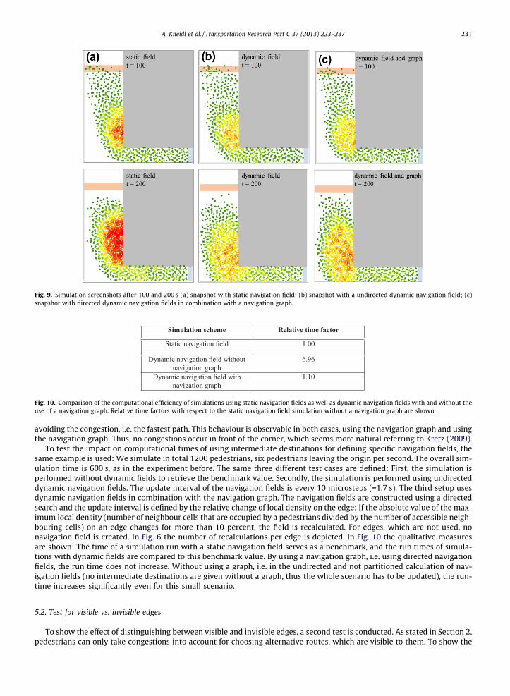
Fig. 9. Simulation screenshots after 100 and 200 s (a) snapshot with static navigation field; (b) snapshot with a undirected dynamic navigation field; (c)snapshot with directed dynamic navigation fields in combination with a navigation graph.

Fig. 10. Comparison of the computational efficiency of simulations using static navigation fields as well as dynamic navigation fields with and without theuse of a navigation graph. Relative time factors with respect to the static navigation field simulation without a navigation graph are shown.

A. Kneidl et al. / Transportation Research Part C 37 (2013) 223–237 231

avoiding the congestion, i.e. the fastest path. This behaviour is observable in both cases, using the navigation graph and usingthe navigation graph. Thus, no congestions occur in front of the corner, which seems more natural referring to Kretz (2009).

To test the impact on computational times of using intermediate destinations for defining specific navigation fields, thesame example is used: We simulate in total 1200 pedestrians, six pedestrians leaving the origin per second. The overall sim-ulation time is 600 s, as in the experiment before. The same three different test cases are defined: First, the simulation isperformed without dynamic fields to retrieve the benchmark value. Secondly, the simulation is performed using undirecteddynamic navigation fields. The update interval of the navigation fields is every 10 microsteps (=1.7 s). The third setup usesdynamic navigation fields in combination with the navigation graph. The navigation fields are constructed using a directedsearch and the update interval is defined by the relative change of local density on the edge: If the absolute value of the max-imum local density (number of neighbour cells that are occupied by a pedestrians divided by the number of accessible neigh-bouring cells) on an edge changes for more than 10 percent, the field is recalculated. For edges, which are not used, nonavigation field is created. In Fig. 6 the number of recalculations per edge is depicted. In Fig. 10 the qualitative measuresare shown: The time of a simulation run with a static navigation field serves as a benchmark, and the run times of simula-tions with dynamic fields are compared to this benchmark value. By using a navigation graph, i.e. using directed navigationfields, the run time does not increase. Without using a graph, i.e. in the undirected and not partitioned calculation of nav-igation fields (no intermediate destinations are given without a graph, thus the whole scenario has to be updated), the run-time increases significantly even for this small scenario.

5.2. Test for visible vs. invisible edges

To show the effect of distinguishing between visible and invisible edges, a second test is conducted. As stated in Section 2,pedestrians can only take congestions into account for choosing alternative routes, which are visible to them. To show the

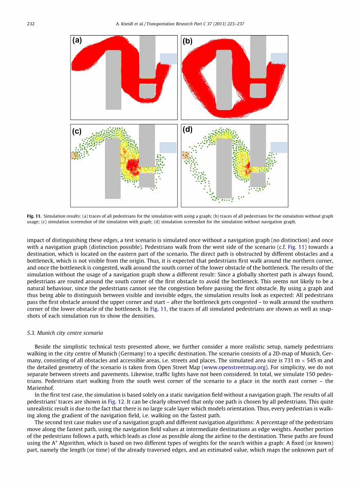
Fig. 11. Simulation results: (a) traces of all pedestrians for the simulation with using a graph; (b) traces of all pedestrians for the simulation without graphusage; (c) simulation screenshot of the simulation with graph; (d) simulation screenshot for the simulation without navigation graph.

232 A. Kneidl et al. / Transportation Research Part C 37 (2013) 223–237

impact of distinguishing these edges, a test scenario is simulated once without a navigation graph (no distinction) and oncewith a navigation graph (distinction possible). Pedestrians walk from the west side of the scenario (c.f. Fig. 11) towards adestination, which is located on the eastern part of the scenario. The direct path is obstructed by different obstacles and abottleneck, which is not visible from the origin. Thus, it is expected that pedestrians first walk around the northern corner,and once the bottleneck is congested, walk around the south corner of the lower obstacle of the bottleneck. The results of thesimulation without the usage of a navigation graph show a different result: Since a globally shortest path is always found,pedestrians are routed around the south corner of the first obstacle to avoid the bottleneck. This seems not likely to be anatural behaviour, since the pedestrians cannot see the congestion before passing the first obstacle. By using a graph andthus being able to distinguish between visible and invisible edges, the simulation results look as expected: All pedestrianspass the first obstacle around the upper corner and start – after the bottleneck gets congested – to walk around the southerncorner of the lower obstacle of the bottleneck. In Fig. 11, the traces of all simulated pedestrians are shown as well as snap-shots of each simulation run to show the densities.

5.3. Munich city centre scenario

Beside the simplistic technical tests presented above, we further consider a more realistic setup, namely pedestrianswalking in the city centre of Munich (Germany) to a specific destination. The scenario consists of a 2D-map of Munich, Ger-many, consisting of all obstacles and accessible areas, i.e. streets and places. The simulated area size is 731 m � 545 m andthe detailed geometry of the scenario is taken from Open Street Map (www.openstreetmap.org). For simplicity, we do notseparate between streets and pavements. Likewise, traffic lights have not been considered. In total, we simulate 150 pedes-trians. Pedestrians start walking from the south west corner of the scenario to a place in the north east corner – theMarienhof.

In the first test case, the simulation is based solely on a static navigation field without a navigation graph. The results of allpedestrians’ traces are shown in Fig. 12. It can be clearly observed that only one path is chosen by all pedestrians. This quiteunrealistic result is due to the fact that there is no large scale layer which models orientation. Thus, every pedestrian is walk-ing along the gradient of the navigation field, i.e. walking on the fastest path.

The second test case makes use of a navigation graph and different navigation algorithms: A percentage of the pedestriansmove along the fastest path, using the navigation field values at intermediate destinations as edge weights. Another portionof the pedestrians follows a path, which leads as close as possible along the airline to the destination. These paths are foundusing the A* Algorithm, which is based on two different types of weights for the search within a graph: A fixed (or known)part, namely the length (or time) of the already traversed edges, and an estimated value, which maps the unknown part of

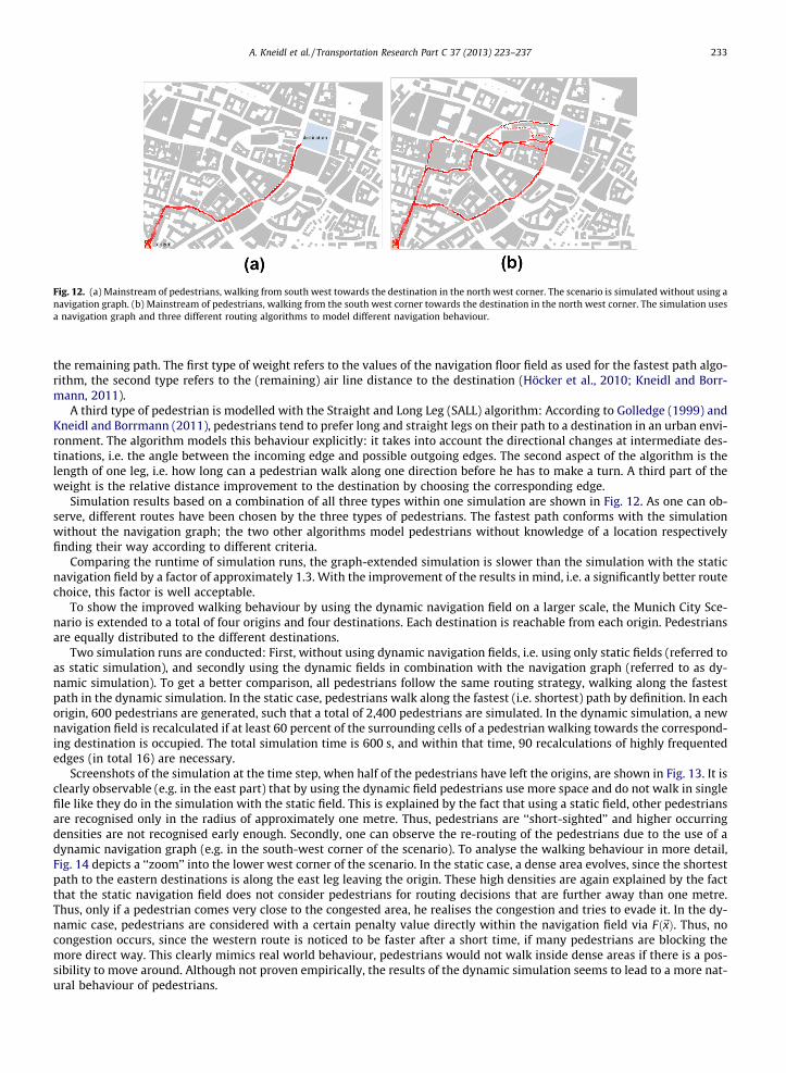
Fig. 12. (a) Mainstream of pedestrians, walking from south west towards the destination in the north west corner. The scenario is simulated without using anavigation graph. (b) Mainstream of pedestrians, walking from the south west corner towards the destination in the north west corner. The simulation usesa navigation graph and three different routing algorithms to model different navigation behaviour.

A. Kneidl et al. / Transportation Research Part C 37 (2013) 223–237 233

the remaining path. The first type of weight refers to the values of the navigation floor field as used for the fastest path algo-rithm, the second type refers to the (remaining) air line distance to the destination (Höcker et al., 2010; Kneidl and Borr-mann, 2011).

A third type of pedestrian is modelled with the Straight and Long Leg (SALL) algorithm: According to Golledge (1999) andKneidl and Borrmann (2011), pedestrians tend to prefer long and straight legs on their path to a destination in an urban envi-ronment. The algorithm models this behaviour explicitly: it takes into account the directional changes at intermediate des-tinations, i.e. the angle between the incoming edge and possible outgoing edges. The second aspect of the algorithm is thelength of one leg, i.e. how long can a pedestrian walk along one direction before he has to make a turn. A third part of theweight is the relative distance improvement to the destination by choosing the corresponding edge.

Simulation results based on a combination of all three types within one simulation are shown in Fig. 12. As one can ob-serve, different routes have been chosen by the three types of pedestrians. The fastest path conforms with the simulationwithout the navigation graph; the two other algorithms model pedestrians without knowledge of a location respectivelyfinding their way according to different criteria.

Comparing the runtime of simulation runs, the graph-extended simulation is slower than the simulation with the staticnavigation field by a factor of approximately 1.3. With the improvement of the results in mind, i.e. a significantly better routechoice, this factor is well acceptable.

To show the improved walking behaviour by using the dynamic navigation field on a larger scale, the Munich City Sce-nario is extended to a total of four origins and four destinations. Each destination is reachable from each origin. Pedestriansare equally distributed to the different destinations.

Two simulation runs are conducted: First, without using dynamic navigation fields, i.e. using only static fields (referred toas static simulation), and secondly using the dynamic fields in combination with the navigation graph (referred to as dy-namic simulation). To get a better comparison, all pedestrians follow the same routing strategy, walking along the fastestpath in the dynamic simulation. In the static case, pedestrians walk along the fastest (i.e. shortest) path by definition. In eachorigin, 600 pedestrians are generated, such that a total of 2,400 pedestrians are simulated. In the dynamic simulation, a newnavigation field is recalculated if at least 60 percent of the surrounding cells of a pedestrian walking towards the correspond-ing destination is occupied. The total simulation time is 600 s, and within that time, 90 recalculations of highly frequentededges (in total 16) are necessary.

Screenshots of the simulation at the time step, when half of the pedestrians have left the origins, are shown in Fig. 13. It isclearly observable (e.g. in the east part) that by using the dynamic field pedestrians use more space and do not walk in singlefile like they do in the simulation with the static field. This is explained by the fact that using a static field, other pedestriansare recognised only in the radius of approximately one metre. Thus, pedestrians are ‘‘short-sighted’’ and higher occurringdensities are not recognised early enough. Secondly, one can observe the re-routing of the pedestrians due to the use of adynamic navigation graph (e.g. in the south-west corner of the scenario). To analyse the walking behaviour in more detail,Fig. 14 depicts a ‘‘zoom’’ into the lower west corner of the scenario. In the static case, a dense area evolves, since the shortestpath to the eastern destinations is along the east leg leaving the origin. These high densities are again explained by the factthat the static navigation field does not consider pedestrians for routing decisions that are further away than one metre.Thus, only if a pedestrian comes very close to the congested area, he realises the congestion and tries to evade it. In the dy-namic case, pedestrians are considered with a certain penalty value directly within the navigation field via Fð~xÞ. Thus, nocongestion occurs, since the western route is noticed to be faster after a short time, if many pedestrians are blocking themore direct way. This clearly mimics real world behaviour, pedestrians would not walk inside dense areas if there is a pos-sibility to move around. Although not proven empirically, the results of the dynamic simulation seems to lead to a more nat-ural behaviour of pedestrians.

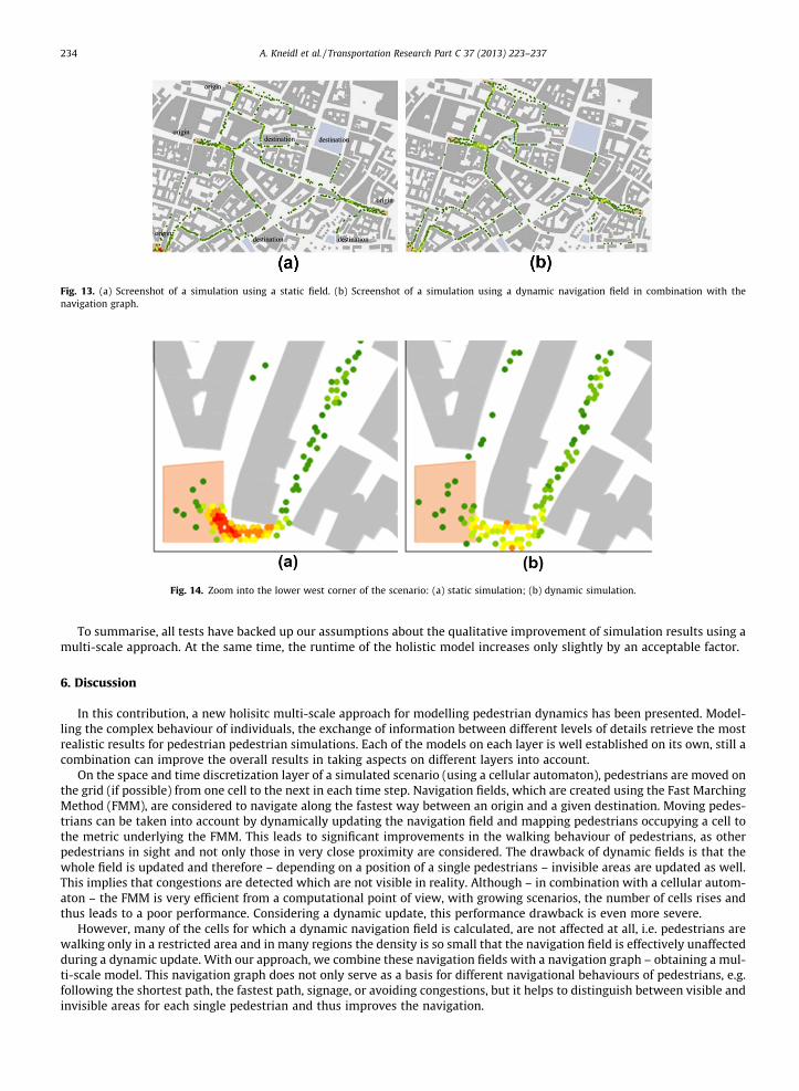
Fig. 13. (a) Screenshot of a simulation using a static field. (b) Screenshot of a simulation using a dynamic navigation field in combination with thenavigation graph.

Fig. 14. Zoom into the lower west corner of the scenario: (a) static simulation; (b) dynamic simulation.

234 A. Kneidl et al. / Transportation Research Part C 37 (2013) 223–237

To summarise, all tests have backed up our assumptions about the qualitative improvement of simulation results using amulti-scale approach. At the same time, the runtime of the holistic model increases only slightly by an acceptable factor.

6. Discussion

In this contribution, a new holisitc multi-scale approach for modelling pedestrian dynamics has been presented. Model-ling the complex behaviour of individuals, the exchange of information between different levels of details retrieve the mostrealistic results for pedestrian pedestrian simulations. Each of the models on each layer is well established on its own, still acombination can improve the overall results in taking aspects on different layers into account.

On the space and time discretization layer of a simulated scenario (using a cellular automaton), pedestrians are moved onthe grid (if possible) from one cell to the next in each time step. Navigation fields, which are created using the Fast MarchingMethod (FMM), are considered to navigate along the fastest way between an origin and a given destination. Moving pedes-trians can be taken into account by dynamically updating the navigation field and mapping pedestrians occupying a cell tothe metric underlying the FMM. This leads to significant improvements in the walking behaviour of pedestrians, as otherpedestrians in sight and not only those in very close proximity are considered. The drawback of dynamic fields is that thewhole field is updated and therefore – depending on a position of a single pedestrians – invisible areas are updated as well.This implies that congestions are detected which are not visible in reality. Although – in combination with a cellular autom-aton – the FMM is very efficient from a computational point of view, with growing scenarios, the number of cells rises andthus leads to a poor performance. Considering a dynamic update, this performance drawback is even more severe.

However, many of the cells for which a dynamic navigation field is calculated, are not affected at all, i.e. pedestrians arewalking only in a restricted area and in many regions the density is so small that the navigation field is effectively unaffectedduring a dynamic update. With our approach, we combine these navigation fields with a navigation graph – obtaining a mul-ti-scale model. This navigation graph does not only serve as a basis for different navigational behaviours of pedestrians, e.g.following the shortest path, the fastest path, signage, or avoiding congestions, but it helps to distinguish between visible andinvisible areas for each single pedestrian and thus improves the navigation.

A. Kneidl et al. / Transportation Research Part C 37 (2013) 223–237 235

The interaction of the two layers allows to use synergy effects: Using intermediate destinations of the navigation graph,we can minimise the area that has to be recalculated dynamically in order to keep the dynamic navigation field updated.Furthermore, a directed search can be conducted by sorting the cells relative to the smallest time and distance to the originrather than the arrival times of the wave as in the original FMM. By initialising a recalculation of floor fields via directed FMMonly if a threshold density is reached and stopping once a navigation field has been calculated for all cells occupied by pedes-trians, the computational efficiency can be further increased. The graph on the other hand can use the derived values of thenavigation fields to assign travel times as edge weights. Using these values leads to a robust measure of travel times, sincelocal congestions and resulting detours are taken into account.

The results presented in this work support the expected theoretical considerations. By realising the combination of thetwo layers, the simulation has improved significantly. Not only the walking behaviour of pedestrians has been improved,i.e. the effect of walking in single file is resolved as well as a more natural route choice due to distinction between visibleand invisible edges, but also computational effort can be minimised by defining smaller navigation fields, respectively.The overall computation time compared to classical approaches using static floor field based navigation is increased onlymildly.

This model therefore provides an extremely realistic and fast computational method to simulate large pedestrian crowdsin real-time. However, effort still has to be made to further improve the details of the model. As we are using a graph, pedes-trians can be only re-routed at intermediate destinations. This is a limitation, as the intermediate destination is sometimescongested. A definition of different criteria to re-route may be one possibility. Another open point is the shape of the inter-mediate destination. Which shape works best for which scenario? Secondly, validation of the model is an ongoing task. Thedifferent route choice algorithms have to be tested on different set-ups (e.g. urban environment, public buildings, largeevents) and calibrated, respectively. Unfortunately not sufficient real data exists to push validation further, at least not so far.

Appendix A. Fast marching method

Given a discretization of X, e.g. the dual grid of cells used in microscopic pedestrian simulators based on cellular auto-mata, the Fast Marching Method ([FMM,]Sethian, 1999) offers an efficient technique so solve the Eikonal Eq. (EIK). Let usshortly recapitulate the main idea of the FMM, which is based on the concept of causality. Vertexes~xi of the computationalgrid underlying the FMM are grouped in three states: far away (no Tð~xiÞ assigned), trial (Tð~xiÞ assigned but not fixed) andfixed (Tð~xiÞ assigned and fix). Starting with a discretization of the initial front, the trial vertex ~xi of the computational gridwith the smallest time Tð~xiÞ is chosen and set to fixed. Its trial neighbours are updated, i.e. T is recalculated, and its furtheraway neighbours are initialised, i.e. T is calculated, and moved to the trial set. These steps are then repeated for the trial ver-tex with the smallest T. The algorithms stops if the trial set is empty or if appropriate stopping criteria are reached, e.g. for allcells~xi occupied by a pedestrian a Tð~xiÞ, i.e. a navigation field, has been calculated. Thus, the FMM is basically nothing elseother than a classical sorting algorithm iteratively finding the trial vertex with the smallest time T, moving this vertex to theset of fixed vertexes and updating its neighbours. Thus adapting an efficient implementation of a sorting algorithm, e.g. aheap sort, the FMM has an optimal computational complexity of N log N (Sethian, 1999).

Appendix B. Automatic construction of large-scale graphs

The automatic construction of navigation graphs consist of two steps. Firstly, appropriate nodes are determined and sec-ondly these are linked via edges. For completeness the construction is summarised and for more details we refer to Kneidlet al. (2011).

B.1. Automatic derivation of a navigation graph

To automatically derive a navigation graph form a given geometry, first navigation points are placed. These points refer tovertices within the resulting graph. They are placed at the bisector of every convex corner of each obstacle with a certaindistance to the corner.

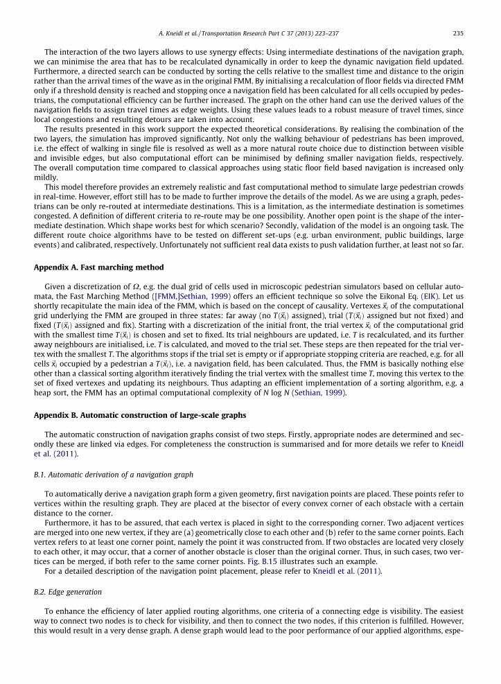
Furthermore, it has to be assured, that each vertex is placed in sight to the corresponding corner. Two adjacent verticesare merged into one new vertex, if they are (a) geometrically close to each other and (b) refer to the same corner points. Eachvertex refers to at least one corner point, namely the point it was constructed from. If two obstacles are located very closelyto each other, it may occur, that a corner of another obstacle is closer than the original corner. Thus, in such cases, two ver-tices can be merged, if both refer to the same corner points. Fig. B.15 illustrates such an example.

For a detailed description of the navigation point placement, please refer to Kneidl et al. (2011).

B.2. Edge generation

To enhance the efficiency of later applied routing algorithms, one criteria of a connecting edge is visibility. The easiestway to connect two nodes is to check for visibility, and then to connect the two nodes, if this criterion is fulfilled. However,this would result in a very dense graph. A dense graph would lead to the poor performance of our applied algorithms, espe-

Fig. B.15. Example for two geometrically close vertices that can be merged, as they refer to the same corner points.

236 A. Kneidl et al. / Transportation Research Part C 37 (2013) 223–237

cially if edges are supercilious. We define supercilious edges as geometrically close edges, i.e. outgoing edges which enclose avery small angle. Edges, which do not lead towards the destination, are considered supercilious as well.

Therefore, the following criteria are introduced: The angle between two outgoing edges can guarantee that no geomet-rically close edges are inserted. By choosing the angle size, the density of a graph can be controlled. Keil and Gutwin (1992)describe such graphs as Fixed-Angle-h graph. The smaller the angle, the denser is the resulting graph.

To avoid edges that are not leading towards the destination, a directed search is conducted. By applying a spatial indexthat stores all geometric elements of a scenario, a nearest-neighbour range search is used to find vertices in direction to thedestination. The details of the search technique can be found in Beckmann et al. (1990). The description of the whole algo-rithm, called cone-based search method, can be found in Kneidl et al. (2011).

References

Antonini, G., Bierlaire, M., Weber, M., 2006. Discrete choice models of pedestrian walking behavior. Transportation Research Part B: Methodological 40 (8),667–687. http://dx.doi.org/10.1016/j.trb.2005.09.006, ISSN: 0191-2615.

Asano, M., Iryo, T., Kuwahara, M., 2010. Microscopic pedestrian simulation model combined with a tactical model for route choice behaviour. TransportationResearch Part C: Emerging Technologies 18 (6), 842–855, ISSN: 0968-090X.

Beckmann, N., Kriegel, H.-P., Schneider, R., Seeger, B., 1990. The R⁄-tree: an efficient and robust access method for points and rectangles. SIGMOD Record 19(2), 322–331, ISSN: 0163-5808.

Blue, V.J., Adler, J.L., 2001. Cellular automata microsimulation for modeling bi-directional pedestrian walkways. Transportation Research Part B:Methodological 35 (3), 293–312. http://dx.doi.org/10.1016/S0191-2615(99)00052-1, ISSN: 0191-2615.

Burstedde, C., Klauck, K., Schadschneider, A., Zittartz, J., 2001. Simulation of pedestrian dynamics using a two-dimensional cellular automaton. Physica A:Statistical Mechanics and its Applications 295 (3–4), 507–525, ISSN: 0378-4371.

Chraibi, M., Seyfried, A., Schadschneider, A., 2010. Generalized centrifugal force model for pedestrian dynamics. Physical Review E 82, 046111.Chraibi, M., Wagoum, U.K., Schadschneider, A., Seyfried, A., 2011a. Force-based models of pedestrian dynamics. Networks and Heterogeneous Media 6, 425–

442.Chraibi, M., Kemloh, U., Schadschneider, A., Seyfried, A., 2011b. Force-based models of pedestrian dynamics. Networks and Heterogeneous Media 6, 425–

442.Dijkstra, E.W., 1959. A note on two problems in connexion with graphs. Numerical Mathematics 1 (1), 269, ISSN: 0029-599X.Dijkstra, J., Jessurun, A.J., Vries, B.d., Timmermans, H.J.P., 2006. Agent architecture for simulating pedestrians in the built environment. In: Bazzan, A.L.,

Chaib-draa, B., Klügl, F., Ossowski, S. (Eds.), Forth Internation Workshop on Agents in Traffic and Transportation (ATT2006), New York, pp. 8–16.Ding, Q., Wang, X., Shan, Q., Zhang, X., 2011. Modeling and Simulation of Rail Transit Pedestrian Flow. Journal of Transportation Systems Engineering and

Information Technology 11 (5), 99–106, ISSN: 1570-6672.Funge, J., Tu, X., Terzopoulos, D., 1999. Cognitive modeling: knowledge, reasoning and planning for intelligent characters. In: Proceedings of the 26th Annual

Conference on Computer Graphics and Interactive Techniques, SIGGRAPH ’99. ACM Press/Addison-Wesley Publishing Co, New York and NY and USA, pp.29–38, ISBN: 0-201-48560-5, doi:10.1145/311535.311538.

Gloor, C., Stucki, P., Nagel, K., 2004. Hybrid Techniques for Pedestrian Simulations. In: Sloot, P., Chopard, B., Hoekstra, A. (Eds.), Cellular Automata, LectureNotes in Computer Science, vol. 3305. Springer, pp. 581–590.

Golledge, R.G., 1999. Wayfinding Behavior: Cognitive Mapping and Other Spatial Processes. Johns Hopkins Univ. Press, Baltimore, ISBN: 080185993X.Gunnar G., L., 1998. Models of wayfinding in emergency evacuations. European Journal of Operational Research 105 (3) (1998) 371–389. doi:10.1016/

S0377-2217(97)00084-2 (ISSN: 0377-2217).Guo, R.-Y., Huang, H.-J., 2012. Formulation of pedestrian movement in microscopic models with continuous space representation. Transportation Research

Part C: Emerging Technologies 24 (0), 50–61. http://dx.doi.org/10.1016/j.trc.2012.02.004, ISSN: 0968-090X.Guo, R.-Y., Huang, H.-J., Wong, S.C., 2011. Collection, spillback, and dissipation in pedestrian evacuation: A network-based method. Transportation Research

Part B: Methodological 45 (3), 490–506. http://dx.doi.org/10.1016/j.trb.2010.09.009, ISSN: 0191-2615.Haklay, M., O’Sullivan, D., Thurstain-Goodwin, M., Schelhorn, T., 2001. ‘‘So go downtown: simulating pedestrian movement in town centres. Environment

and Planning B: Planning and Design 28 (3), 343–359.Hamacher, H.W., Tjandra, S.A., 2002. Mathematical modelling of evacuation problems: A state of the art. In: Schreckenberg, M. (Ed.), Pedestrian and

Evacuation Dynamics. Springer, Berlin, pp. 227–266, ISBN: 978-3540426905.Hartmann, D., 2010. Adaptive pedestrian dynamics based on geodesics. New Journal of Physics 12 (4), 043032.Helbing, D., 1992. A fluid-dynamic model for the movement of pedestrians. Complex Systems 6, 391–415.Helbing, D., Molnár, P., 1995. Social Force Model for Pedestrian Dynamics. Physical Review E 51 (5), 4282–4286, ISSN: 1063-651X.Henderson, L.F., 1974. On the fluid mechanics of human crowd motion. Transportation Research Part B: Methodological 8 (6), 509–515, ISSN: 0191-2615.Höcker, M., Berkhahn, V., Kneidl, A., Borrmann, A., Klein, W., 2010. Graph-based approaches for simulating pedestrian dynamics in building models. In:

University College Cork (Ed.), 8th European Conference on Product & Process Modelling (ECPPM), Cork and Ireland, 2010.Hoogendoorn, S.P., Bovy, P.H.L., 2004. Pedestrian route-choice and activity scheduling theory and models. Transportation Research Part B: Methodological

38 (2), 169–190, ISSN: 0191-2615.Keil, J.M., Gutwin, C.A., 1992. Classes of Graphs Which Approximate the Complete Euclidean Graph. Discrete & Computational Geometry 7, 13–28.Kirik, E., Yurgel’yan, T.B., Krouglov, D., 2009. The shortest time and/or the shortest path strategies in a CA FF pedestrian dynamics model. Journal of Siberian

Federal University Mathematics & Physics 2 (3), 271–278.

A. Kneidl et al. / Transportation Research Part C 37 (2013) 223–237 237

Klüpfel, H., 2003. A Cellular Automaton Model for Crowd Movement and Egress Simulation. Ph.D. thesis, Universität Duisburg-Essen, Duisburg.Klüpfel, H., Meyer-König, T., 2004. Simulation of the evacuation of a football stadium. In: Hoogendoorn, S. et al. (Eds.), Traffic and Granular Flow ’03.

Springer, Berlin, pp. 423–430.Kneidl, A., Borrmann, A., 2011. How do pedestrians find their way? Results of an experimental study with students compared to simulation results. In:

Jaskolowski, W., Kepka, P. (Eds.), EMEVAC, The Main School of Fire Service, Warsaw.Kneidl, A., Borrmann, A., Hartmann, D., 2011. Generating sparse navigation graphs for microscopic pedestrian simulation models. In: Hartmann, T., de Wilde,

P., Rafiq, Y. (Eds.), Proceedings of the 2011 eg-ice Workshop, ISBN: 978-90-365-3216-7.Köster, G., Hartmann, D., Klein, W., 2010. Microscopic pedestrian simulations: from passenger exchange times to regional evacuation. In: Operations

Research – Mastering Complexity.Kretz, T., 2009. Pedestrian traffic: on the quickest path. Journal of Statistical Mechanics: Theory and Experiment (03), P03012, ISSN: 1742-5468.Kretz, T., Schreckenberg, M., 2006. F.A.S.T. – floor field- and agent-based simulation tool. In: Chung, E., Barcel’o, J., Dumont, A.-G. (Eds.), International

Symposium of Transport Simulation (ISTS06).Kretz, T., Hengst, S., Rocea, V., Perez Arias, A., Friedberger, S., Hanebeck, U.D., 2011. Calibrating dynamic pedestrian route choice with an extended range

telepresence system. In: 1st IEEE Workshop on Modeling, Simulation and Visual Analysis of Large Crowds.Lakoba, T., Kaup, D., Finkelstein, N., 2005. Modifications of the Helbing-Molnár-Farkas-Vicsek social force model for pedestrian evolution. Simulation 81,

339–352.Lämmel, G., Rieser, M., Nagel, K., 2010. Large scale microscopic evacuation simulation. In: Klingsch, W. (Ed.), Pedestrian and Evacuation Dynamics 2008.

Springer, Berlin and Heidelberg, pp. 547–553, ISBN: 9783642045035.Lerner, A., Chrysanthou, Y., Lischinski, D., 2007. Crowds by Example. Computer Graphics Forum 26 (3), 655–664. http://dx.doi.org/10.1111/j.1467-

8659.2007.01089.x, ISSN: 0167-7055.Löhner, R., 2010. On the modeling of pedestrian motion. Applied Mathematical Modelling 34, 366–382.Loscos, C., Marchal, D., Meyer, A., 2003. Intuitive crowd behaviour in dense urban environments using local laws. In: University of Birmingham (Ed.),

Proceedings of the Theory and Practice of Computer Graphics. IEEE Computer Society, Los Alamitos and Calif., ISBN 0-7695-1942-3, pp. 122–129.Mayer, H., Hartmann, D., Klein, W., 2011. Coupling pedestrian simulation and fire simulation for online evacuation planning. In: Jaskolowski, W., Kepka, P.

(Eds.), EMEVAC, The Main School of Fire Service, Warsaw.Mitchell, D.H., MacGregor Smith, J., 2001. Topological network design of pedestrian networks. Transportation Research Part B: Methodological 35 (2), 107–

135. http://dx.doi.org/10.1016/S0191-261(99)00039-9, ISSN: 0191-2615.Nishinari, K., Kirchner, A., Namazi, A., Schadschneider, A., 2004. Extended floor field CA model for evacuation dynamics. IEICE Transactions on Information

and Systems E87D, 726–732.Parisi, D.R., Gilman, M., Moldovan, H., 2009. A modification of the social force model can reproduce experimental data of pedestrian flows in normal

conditions. Physica A 388, 3600–3608.Pelechano, N., Malkawi, A., 2008. Evacuation simulation models: Challenges in modeling high rise building evacuation with cellular automata approaches.

Automation in Construction 17 (4), 377–385, ISSN: 0926-5805.Petres, C., Pailhas, Y., Patron, P., Petillot, Y., Evans, J., Lane, D., 2007. Path Planning for Autonomous Underwater Vehicles. IEEE Transactions on Robotics 23,

331–341.Reynolds, C., 1999. Steering behaviors for autonomous characters. In: Game Developers Conference.Rindsfüser, G., Klügl, F., 2007. Agent-based pedestrian simulation: a case study of the Bern Railway Station. In: Nagel, K., Koll-Schretzenmayr, M. (Eds.), disP,

vol. 170, ETH Zürich, Zurich and Switzerland, pp. 9–18.Robin, T., Antonini, G., Bierlaire, M., Cruz, J., 2009. Specification, estimation and validation of a pedestrian walking behavior model. Transportation Research

Part B: Methodological 43 (1), 36–56. http://dx.doi.org/10.1016/j.trb.2008.06.010, ISSN: 0191-2615.Rodriguez, S., Amato, N.M., 2010. Behavior-based evacuation planning. In: Proceedings of 2010 IEEE International Conference on Robotics and Automation,

Anchorage.Ronald, N., Sterling, L., Kirley, M., 2007. An Agent-Based Approach To Modelling Pedestrian Behaviour. Lecture Notes in Computer Science, 145–156.Schadschneider, A., Klingsch, W., Klüpfel, H., Kretz, T., Rogsch, C., Seyfried, A., 2009. Evacuation dynamics: Empirical results, modeling and applications.

Encyclopedia of Complexity and System Science, 3142–3176.Sethian, J.A., 1999. Level Set Methods and Fast Marching Methods. Cambridge University Press.Shi, C., Zhong, M., Nong, X., He, L., Shi, J., Feng, G., 2012. Modeling and safety strategy of passenger evacuation in a metro station in China. Safety Science 50

(5), 1319–1332, ISSN: 0925-7535.Sud, A., Andersen, E., Curtis, S., Lin, M.C., Manocha, D., 2008. Real-Time Path Planning in Dynamic Virtual Environments Using Multiagent Navigation Graphs.

IEEE Transactions on Visualization and Computer Graphics 14, 526–538, ISSN: 1077-2626.Teknomo, K., 2008. Modeling mobile traffic agents on network simulation. In: Transportation Science Society of the Phillippines 2008 – Proceedings of the

16th Annual of Transportation Science.Teknomo, K., Fernandez, P., 2012. Simulating optimum egress time. Safety Science 50 (5), 1228–1236. http://dx.doi.org/10.1016/j.ssci.2011.12.025, ISSN:

0925-7535.Teknomo, K., Millonig, R., 2007. A navigation algorithm for pedestrian simulation in dynamic environments. In: Proceedings of the 11th World Conference

on Transport Research (WCTR), Berkeley and USA.Varas, A., Cornejo, M.D., Mainemer, D., Toledo, B., Rogan, J., Munoz, V., Valdivia, J.A., 2007. Cellular automaton model for evacuation process with obstacles.

Physica A: Statistical Mechanics and its Applications 382 (2), 631–642, ISSN: 0378-4371.Wagoum, U.K., Seyfried, A., Holl, S., 2012. Modelling dynamic route choice of pedestrians to assess the criticality of building evacuation. Advances in

Complex Systems.Weidmann, U., 1993. Transporttechnik der Fussgänger: Transporttechnische Eigenschaften des Fussgängerverkehrs (Literaturauswertung).Yamamoto, K., Kokubo, S., Nishinari, K., 2007. Simulation for pedestrian dynamics by real-coded cellular automata. Physica A: Statistical Mechanics and its

Applications 379 (2), 654. http://dx.doi.org/10.1016/j.physa.2007.02.040, ISSN: 0378-4371.Yu, W., Chen, R., Dong, L., Dai, S., 2005. Centrifugal force model for pedestrian dynamics. Physical Review E 72, 026112.Zhang, Q., Han, B., Li, D., 2008. Modeling and simulation of passenger alighting and boarding movement in Beijing metro stations. Transportation Research

Part C: Emerging Technologies 16 (5), 635–649. http://dx.doi.org/10.1016/j.trc.2007.12.001, ISSN: 0968-090X.