a hybrid fault-tolerant algorithm for mpls network - university of
TRANSCRIPT
Technical Report
A Hybrid Fault-Tolerant Algorithm for MPLS Networks
Maria Hadjiona, Chryssis Georgiou, Maria Papa, Vasos Vassiliou
University of Cyprus
Computer Science Department
TR – 07 – 06
December 2007

ii
Abstract In this report we present a new fault tolerant, path maintaining, algorithm for use in
MPLS based networks. The novelty of the algorithm lies upon the fact that it is the first to
employ both path restoration mechanisms typically used in MPLS networks: protection
switching and dynamic path rerouting. In addition, it is the first algorithm to adequately
satisfy all four criteria which we consider very important for the performance of the
restoration mechanisms in MPLS networks: fault recovery time, packet loss, packet
reordering and tolerance of multiple faults. Simulation results indicate the performance
advantages of the proposed hybrid algorithm (with respect to the four criteria), when
compared with other algorithms that employ only one of the two restoration mechanisms.

iii
Table of contents
1 INTRODUCTION............................................................................................................................... 1 1.1 BACKGROUND.............................................................................................................................. 2
1.1.1 What is MPLS ......................................................................................................................... 2 1.1.2 Fault tolerance in MPLS ........................................................................................................ 4
1.2 MOTIVATION................................................................................................................................ 6 1.3 CONTRIBUTIONS........................................................................................................................... 6 1.4 DOCUMENT ORGANIZATION......................................................................................................... 7
2 RELATED WORK ............................................................................................................................. 8 2.1 EXISTING MPLS RECOVERY ALGORITHMS ................................................................................... 8
2.1.1 Protection switching algorithms............................................................................................. 8 2.1.2 Rerouting algorithms.............................................................................................................19
2.2 COMPARISON OF EXISTING MPLS RECOVERY ALGORITHMS .......................................................30 2.2.1 Fault Recovery time...............................................................................................................31 2.2.2 Packet Loss ............................................................................................................................33 2.2.3 Packet Reordering .................................................................................................................34 2.2.4 Multiple Fault Tolerance.......................................................................................................35 2.2.5 Comparison Summary ...........................................................................................................36
3 HYBRID ALGORITHM...................................................................................................................38 3.1 FAULT DETECTION AND FAULT NOTIFICATION ...........................................................................38 3.2 RESTORATION AND NOTIFICATION..............................................................................................38 3.3 ALGORITHM DESCRIPTION ..........................................................................................................39 3.4 OUTLINE OF THE ALGORITHM......................................................................................................41 3.5 EXAMPLE OF HYBRID ALGORITHM ..............................................................................................42
4 SIMULATION AND ANALYSIS.....................................................................................................46 4.1 NETWORK SIMULATOR 2.............................................................................................................46 4.2 SCENARIOS..................................................................................................................................47 4.3 SIMPLE AND SPARSE TOPOLOGY ..................................................................................................49 4.4 SIMPLE AND DENSE TOPOLOGY ...................................................................................................56 4.5 COMPLEX AND SPARSE TOPOLOGY ..............................................................................................63 4.6 COMPLEX AND DENSE TOPOLOGY ...............................................................................................70 4.7 ANALYSIS OF RESULTS................................................................................................................77
5 CONCLUSION ..................................................................................................................................81 6 FUTURE WORK...............................................................................................................................82 REFERENCES ............................................................................................................................................83

iv
List of figures FIGURE 1.1: MPLS SHIM HEADER ................................................................................................................... 2 FIGURE 1.2: MPLS DOMAIN ............................................................................................................................ 3 FIGURE 1.3: LABEL SWITCH PATH ................................................................................................................... 3 FIGURE 1.4: LOCAL REPAIR ............................................................................................................................. 5 FIGURE 1.5: GLOBAL REPAIR........................................................................................................................... 5 FIGURE 2.1: EXAMPLE OF HASKIN'S PROPOSAL............................................................................................... 9 FIGURE 2.2: EXAMPLE OF MAKAM'S PROPOSAL .............................................................................................. 9 FIGURE 2.3: EXAMPLE OF GONFA ALGORITHM WHEN THE BACKWARD LSP IS USED......................................11 FIGURE 2.4: THE INFLUENCED FLOW IS ROUTED DIRECTLY TO THE ALTERNATIVE PATH ................................11 FIGURE 2.5: EXAMPLE OF TWO PATH ALGORITHM .........................................................................................14 FIGURE 2.6: EXAMPLE OF RBPC ALGORITHM (LOCAL) ..................................................................................15 FIGURE 2.7: EXAMPLE OF RBPC ALGORITHM (GLOBAL) ...............................................................................15 FIGURE 2.8: EXAMPLE OF DUAL ALGORITHM.................................................................................................16 FIGURE 2.9: EXAMPLE MBAK ALGORITHM ...................................................................................................17 FIGURE 2.10: EXAMPLE OF SPM ALGORITHM ................................................................................................18 FIGURE 2.11: EXAMPLE OF DYNAMIC ROUTING ALGORITHM ........................................................................19 FIGURE 2.12: EXAMPLE OF A.J.C ALGORITHM ...............................................................................................20 FIGURE 2.13: EXAMPLE OF YOON ALGORITHM ..............................................................................................21 FIGURE 2.14: EXAMPLE OF CHEN & OH PROPOSAL........................................................................................22 FIGURE 2.15: A FAULT OCCURS BETWEEN 5 AND 7.........................................................................................24 FIGURE 2.16: (A) THE SPT WITH THE LSR 5 BEING THE ROOT. (Β) THE ARRAY OF LENGTHS.........................24 FIGURE 2.17: (A) THE SPT AFTER THE FAULT. (B) THE ARRAY OF LENGTHS AFTER THE UPDATE. ..................25 FIGURE 2.18: THE INFLUENCED DATA FLOW IS ROUTED THROUGH THE LOCAL ALTERNATIVE PATH...............25 FIGURE 2.19: EXAMPLE OF MIRA ALGORITHM ..............................................................................................27 FIGURE 2.20: FAILURE IS DETECTED IN L19 LINK...........................................................................................28 FIGURE 2.21: RECOVERY FROM THE FAILURE OF LINK L19 ............................................................................28 FIGURE 2.22: CREATION OF THE GRAPH.........................................................................................................29 FIGURE 2.23: MPLS STACK MECHANISM .......................................................................................................30 FIGURE 3.1: OUTLINE OF THE HYBRID ALGORITHM .......................................................................................42 FIGURE 3.2: ROUTE TRAFFIC VIA BACKWARD LSP.........................................................................................43 FIGURE 3.3: ROUTE TRAFFIC DIRECTLY INTO ALTERNATIVE PATH..................................................................43 FIGURE 3.4: (A)SPT BEFORE FAILURE, (B) SPT AFTER FAILURE.....................................................................44 FIGURE 3.5: ALTERNATIVE PATH AFTER 2ND FAILURE ...................................................................................44 FIGURE 3.6: UPDATED SPT ............................................................................................................................45 FIGURE 4.1: NETWORK TOPOLOGIES ..............................................................................................................48 FIGURE 4.2: PACKET LOSS - SIMPLE & SPARSE TOPOLOGY ............................................................................50 FIGURE 4.3: PACKET REORDERING - SIMPLE & SPARSE TOPOLOGY ...............................................................51 FIGURE 4.4: RECEIVED PACKETS - SIMPLE & SPARSE TOPOLOGY ..................................................................51 FIGURE 4.5: THROUGHPUT - SIMPLE & SPARSE TOPOLOGY ............................................................................52 FIGURE 4.6: DELAY TIME - SIMPLE & SPARSE TOPOLOGY..............................................................................52 FIGURE 4.7: DELAY TIME - SIMPLE & SPARSE TOPOLOGY..............................................................................53 FIGURE 4.8: DELAY TIME - SIMPLE & SPARSE TOPOLOGY..............................................................................53 FIGURE 4.9: DELAY TIME - SIMPLE & SPARSE TOPOLOGY..............................................................................54 FIGURE 4.10: DELAY TIME - SIMPLE & SPARSE TOPOLOGY............................................................................54 FIGURE 4.11: RECOVERY TIME - SIMPLE & SPARSE TOPOLOGY .....................................................................56 FIGURE 4.12: PACKET LOSS - SIMPLE & DENSE TOPOLOGY............................................................................57 FIGURE 4.13: PACKET REORDERING- SIMPLE & DENSE TOPOLOGY ...............................................................58 FIGURE 4.14: RECEIVED PACKETS - SIMPLE & DENSE TOPOLOGY..................................................................58 FIGURE 4.15: THROUGHPUT - SIMPLE & DENSE TOPOLOGY ...........................................................................59 FIGURE 4.16: DELAY TIME - SIMPLE & DENSE TOPOLOGY.............................................................................59 FIGURE 4.17: DELAY TIME - SIMPLE & DENSE TOPOLOGY.............................................................................60 FIGURE 4.18: DELAY TIME - SIMPLE & DENSE TOPOLOGY.............................................................................60 FIGURE 4.19: DELAY TIME - SIMPLE & DENSE TOPOLOGY.............................................................................61
v
FIGURE 4.20: RECOVERY TIME.......................................................................................................................63 FIGURE 4.21: PACKET LOSS - COMPLEX & SPARSE TOPOLOGY ......................................................................64 FIGURE 4.22: PACKET REORDERING - COMPLEX & SPARSE TOPOLOGY .........................................................64 FIGURE 4.23: RECEIVED PACKETS - COMPLEX & SPARSE TOPOLOGY ............................................................65 FIGURE 4.24: THROUGHPUT - COMPLEX & SPARSE TOPOLOGY ......................................................................65 FIGURE 4.25: DELAY TIME - COMPLEX & SPARSE TOPOLOGY........................................................................66 FIGURE 4.26: DELAY TIME - COMPLEX & SPARSE TOPOLOGY........................................................................66 FIGURE 4.27: DELAY TIME - COMPLEX & SPARSE TOPOLOGY........................................................................67 FIGURE 4.28: DELAY TIME - COMPLEX & SPARSE TOPOLOGY........................................................................67 FIGURE 4.29: DELAY TIME - COMPLEX & SPARSE TOPOLOGY........................................................................68 FIGURE 4.30: RECOVERY TIME - COMPLEX & SPARSE TOPOLOGY .................................................................70 FIGURE 4.31: PACKET LOSS - COMPLEX & DENSE TOPOLOGY .......................................................................71 FIGURE 4.32: PACKET REORDERING - COMPLEX & DENSE TOPOLOGY...........................................................72 FIGURE 4.33: RECEIVED PACKETS - COMPLEX & DENSE TOPOLOGY..............................................................72 FIGURE 4.34: THROUGHPUT - COMPLEX & DENSE TOPOLOGY .......................................................................73 FIGURE 4.35: DELAY TIME - COMPLEX & DENSE TOPOLOGY.........................................................................73 FIGURE 4.36: DELAY TIME - COMPLEX & DENSE TOPOLOGY.........................................................................74 FIGURE 4.37: DELAY TIME - COMPLEX & DENSE TOPOLOGY.........................................................................74 FIGURE 4.38: DELAY TIME - COMPLEX & DENSE TOPOLOGY.........................................................................75 FIGURE 4.39: DELAY TIME - COMPLEX & DENSE TOPOLOGY.........................................................................75 FIGURE 4.40: RECOVERY TIME- COMPLEX & DENSE TOPOLOGY ...................................................................77

vi
List of Tables TABLE 2.1: ALL POSSIBLE ALTERATIVE PATHS OF MBAK ALGORITHM .........................................................18 TABLE 2.2: THE QUADRUPLES THAT ARE CREATED AT STEP 4 ........................................................................25 TABLE 2.3: COMPARISON OF EXISTING ALGORITHMS .....................................................................................37 TABLE 4.1: IDEAL AND NON IDEAL CASES FOR HYBRID ALGORITHM ..............................................................80 TABLE 4.2: CASES WHERE HYBRID HAVE THE SAME RESULTS AS GONFA AND AS OTEL.................................80
1
1 Introduction The explosive increase of data circulation over the Internet in conjunction with the
complexity of the provided Internet services have negatively affected the quality of
service and the data flow over this global infrastructure. The Multi-Protocol Label
Switching (MPLS) [25] combines the scalability of the IP protocol and the efficiency of
label switching to improve network data circulation.
The protection of data flows in the case of link or router failures is very important,
especially for real time services and multimedia applications. MPLS employs two basic
techniques for network recovery: (i) protection switching, where a pre-computed
alternative path, which is usually disjoint from the working path, is set up for every flow
and (ii) rerouting, where an alternative path is dynamically recomputed after a fault is
detected. For both techniques, the alternative path can be either global or local [26].
The recovery of the MPLS network is based on the algorithm that is applied in order to
detect the faults and route the data flow in an alternative path. There are various
algorithms that have been proposed in the bibliography. Each algorithm employs on of
the two basic techniques.
In this report we propose and evaluate such a hybrid fault-tolerant path-maintaining
algorithm for use in MPLS based networks. It satisfies all four performance criteria and
deploys effectively, in a non-trivial manner, both mechanisms based on the conditions of
the fault, thus exploiting the advantages of each technique. Simulation results
demonstrate the effectiveness of the new approach.
2
1.1 Background
1.1.1 What is MPLS MPLS is a protocol which is used to strength the IP network. When a packet enters the
MPLS network the router that receives it, is responsible to add a label on it. The label is
based on certain criteria’s like the IP address of the recipient and it is used to route the
packet through the next routers. Before the packet leaves the MPLS network, the last
router is responsible to remove the label [7].
The MPLS path is determined only once when the packet enters the MPLS network. The
routers at the length of path do not take any routing decisions they only use the label of
the packet as an index to an array which indicates the next router. Also the router must
switch the label of the packet, before sending it to the next router.
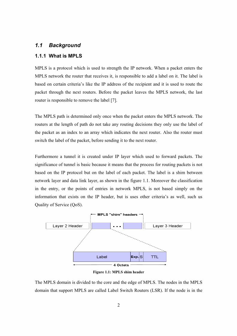
Furthermore a tunnel it is created under IP layer which used to forward packets. The
significance of tunnel is basic because it means that the process for routing packets is not
based on the IP protocol but on the label of each packet. The label is a shim between
network layer and data link layer, as shown in the figure 1.1. Moreover the classification
in the entry, or the points of entries in network MPLS, is not based simply on the
information that exists on the IP header, but is uses other criteria’s as well, such us
Quality of Service (QoS).
Figure 1.1: MPLS shim header
The MPLS domain is divided to the core and the edge of MPLS. The nodes in the MPLS
domain that support MPLS are called Label Switch Routers (LSR). If the node is in the
3
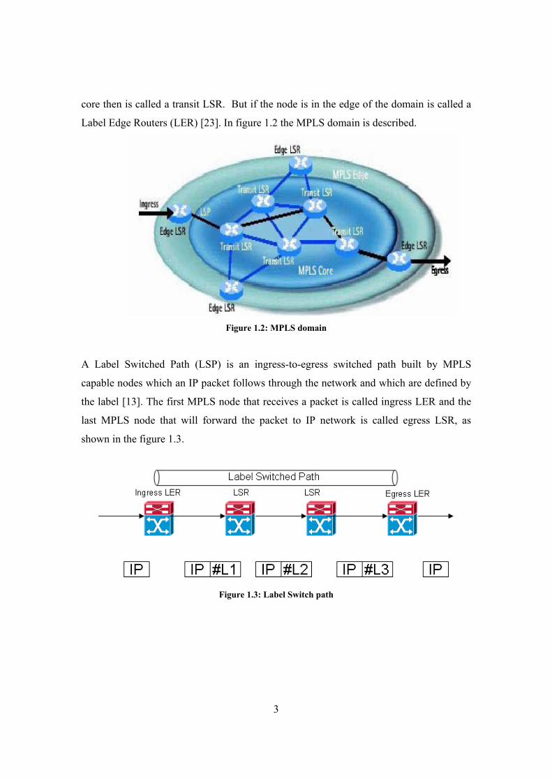
core then is called a transit LSR. But if the node is in the edge of the domain is called a
Label Edge Routers (LER) [23]. In figure 1.2 the MPLS domain is described.
Figure 1.2: MPLS domain
A Label Switched Path (LSP) is an ingress-to-egress switched path built by MPLS
capable nodes which an IP packet follows through the network and which are defined by
the label [13]. The first MPLS node that receives a packet is called ingress LER and the
last MPLS node that will forward the packet to IP network is called egress LSR, as
shown in the figure 1.3.
Figure 1.3: Label Switch path

4
1.1.2 Fault tolerance in MPLS It is very important that when a fault occurs on the existing path the data flow must be
transferred immediately on an alternative path, otherwise a large amount of data will be
lost by the point of the failure. For this reason MPLS provides mechanisms which can
detect the fault early and also techniques which are used to switch the influenced flow in
a path that can route the flow to the destination.
1.1.2.1 Detection of a fault
The fault in a path can be detected with the possessed control that is used between the
neighbors LSRs. For instance KeepAlive messages can be used which are exchanged
periodically between all neighboring routers in the path. The LSR that detects the failure
may be able to switch the flow to the alternative path. If the LSR is not in place to react
immediately, then must send Fault Indication Signal (FIS) messages in order to inform
the others. When the router responsible to reroute the traffic receives FIS messages, then
the procedure of recovering from the failure must start. The FIS messages are transmitted
with high priority so this ensures that FIS will be propagated fast to the LSR which is in
charge to restore the influenced flow [26].
1.1.2.2 Techniques for recovery
There are two basic techniques that are used for the recovery of the MPLS network:
rerouting and protection switching. In rerouting the alternative path is computed
dynamically after the detection of the fault. After the establishment of the alternative
LSP, the data flow is switched to the new path. On the other hand in the protection
switching the alternative path is pre-computed and pre-established and when the fault
occurs, the data flow is routed to that as soon as the fault is detected [26]. Protection
switching provides fast restoration when compared to rerouting technique, since the
alternative path is already established and the switching to it is performed immediately
after the fault is detected. Alternatively, rerouting technique appears to be better in
handling multiple faults as a new alternative path, if needed, is computed dynamically for
each fault.
5
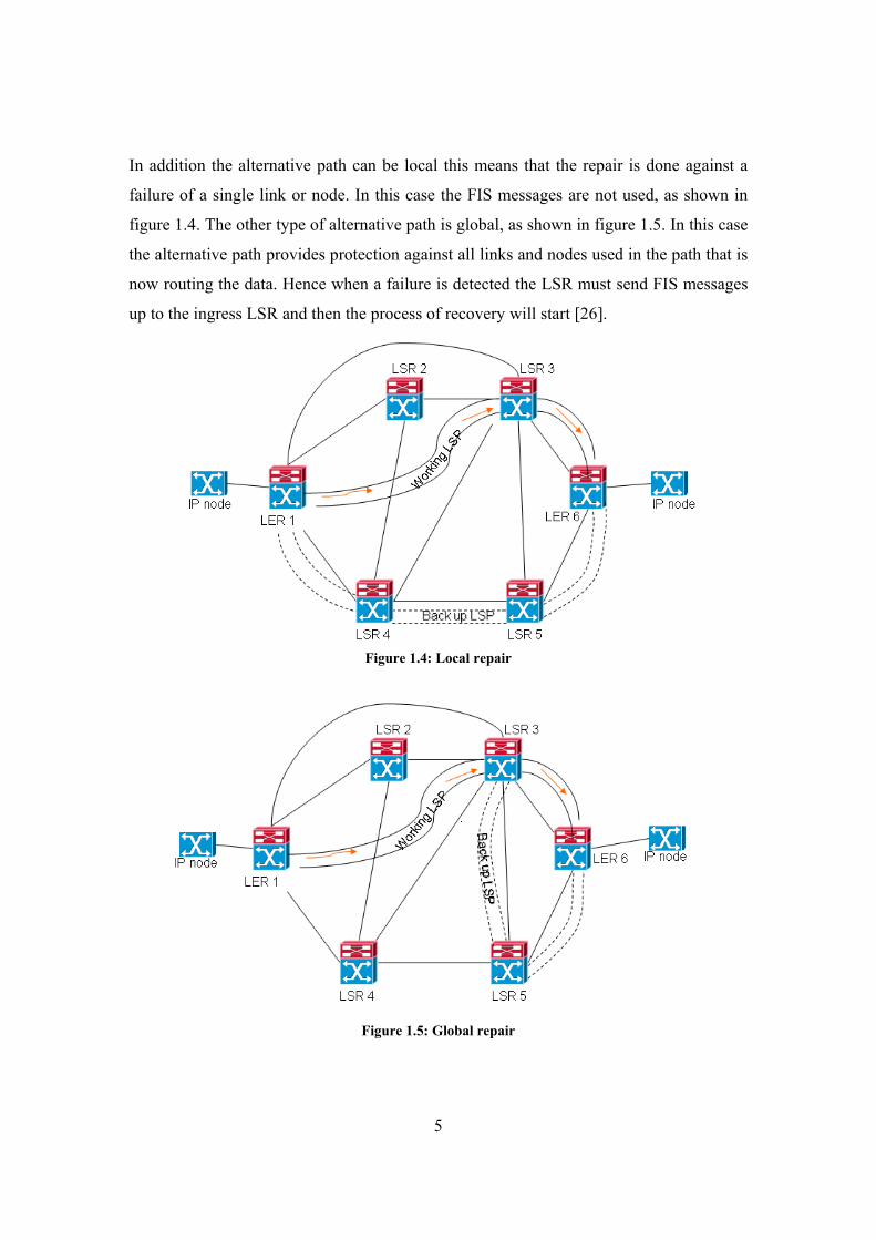
In addition the alternative path can be local this means that the repair is done against a
failure of a single link or node. In this case the FIS messages are not used, as shown in
figure 1.4. The other type of alternative path is global, as shown in figure 1.5. In this case
the alternative path provides protection against all links and nodes used in the path that is
now routing the data. Hence when a failure is detected the LSR must send FIS messages
up to the ingress LSR and then the process of recovery will start [26].
Figure 1.4: Local repair
Figure 1.5: Global repair

6
1.2 Motivation The main motivation for this work is to overcome the drawbacks of the previously
proposed schemes for the restoration mechanism in MPLS networks during link/node
failure. Currently there are many algorithms that can be used to reroute traffic fast when a
fault occurs in the MPLS domain. Each technique presents both advantages and
disadvantages depending on the application or the topology of the network they are
employed upon. Protection switching provides fast restoration when compared to the
rerouting technique, since the alternative path is already established and the switching to
it is performed immediately after the fault is detected. Alternatively, the rerouting
technique appears to be better in handling multiple faults, since a new alternative path, if
needed, is computed dynamically for each fault. A question driven by the comparison of
the two techniques is whether the combination of rerouting and protection switching will
give better results.
We consider fault recovery time, packet loss, packet reordering and the ability to tolerate
multiple faults as the most important criteria to evaluate a fast restoration algorithm in
MPLS networks. To the best of our knowledge there is no current algorithm, either
protection switching or rerouting, able to perform well in all four performance criteria.
The challenge is to find an efficient way to combine the two restoration mechanisms in
order to exploit each method’s strengths and obtain a new hybrid algorithm that would
perform best in all four criteria.
1.3 Contributions
Several service restoration algorithms are proposed for MPLS networks, each employing
one of the two restoration mechanisms. We studied each of these algorithms and
evaluated them (in a theoretical manner) based on the abovementioned four criteria.
Based on the comparison we have selected Gonfa [13] a protection switching algorithm
and Otel [22] a rerouting algorithm, both of them perform well in most criteria. Next, we
combined in a non-trivial manner Gonfa and Otel algorithms in order to satisfy the four

7
selected performance criteria and define the first hybrid algorithm for MPLS networks.
The simulations of the hybrid algorithm on different topologies and different types of
faults have shown that hybrid algorithm is able to detect and recover from any fault.
More specifically the simulation results have demonstrated the efficiency of the new
algorithm and that in most scenarios performs well in all criteria.
1.4 Document Organization Chapter 2 is concerned with the analysis of existing fault tolerance algorithms for MPLS
networks. Also a comparison is presented based on four performance criteria. The Hybrid
algorithm is presented and explained in chapter 3. In the next chapter, gained results and
made tests are illustrated. Chapter 5 presents the conclusion about this project. Finally an
outlook in the future can be found in chapter 6.

8
2 Related Work
In this chapter the different algorithms proposed in the bibliography are presented, along
with the techniques used in order to recover from failures. Firstly the algorithms which
employ protection switching technique are described and then the algorithms with
rerouting technique. Finally the comparison of the existing algorithms is presented based
on four selected performance criteria.
2.1 Existing MPLS recovery algorithms
2.1.1 Protection switching algorithms Haskin algorithm The model provides local restoration of the influenced data flow using the technique of
protection switching. The steps [14] followed to recover a failure are:
1 The alternative path is composed of two portions: the path from the egress LSR to ingress LSR in the reverse direction of the primary/protected path (Backward LSP) and the alternative path from the ingress LSR to the egress LSR (Alternative LSP). The alternative LSP must be completely disjoint with the primary LSP.
2 When the fault occurs, the LSR which detects the failure, routes the data flow
through the backward LSP.
The topology of the figure 2.1 is also used in later examples. The working path in all the
algorithms is established between LSR1, LSR3, LSR5, LSR7, LSR9 and LSR11.
In the figure 2.1 the backward LSP is established between LSR11, LSR9, LSR7, LSR5,
LSR3 and LSR1. The last part of the alternative path is the alternative LSP which is
established between LSR1, LSR2, LSR4, LSR6, LSR8, LSR10 and LSR11. When fault
occurs in LSR5, LSR3 detects the failure and reroutes the incoming traffic in the reverse
direction of the protected path using the backward LSP. When the redirected traffic
reaches the ingress LSR, it is switched to the previously established alternative LSP.
Furthermore, when the ingress LSR detects traffic in the reverse direction it switches the
traffic entering the MPLS domain directly to the alternative LSP.

9
Figure 2.1: Example of Haskin's Proposal
Makam’s Algorithm In this proposal [20] global restoration is used to route the influenced data flow in
combination of protection switching technique. The steps followed to recover a failure
are:
1 The alternative path is set up between the ingress LSR to the egress LSR and must be completely disjoint with the working LSP.
2 When a fault is detected, fault notification mechanism (FIS) is used to convey
information about the occurrence of a fault to a responsible node in order to take the appropriate action (e.g., the ingress LSR is notified to switch traffic from the protected path to the alternative path).
In figure 2.2 the alternative path is established between LSR1, LSR2, LSR4, LSR6,
LSR8, LSR10 and LSR11. When LSR3 detects the failure of the LSR5, then is
responsible to send FIS messages to the ingress LSR. After receiving FIS messages,
LSR1 reroutes the traffic through the alternative path.
Figure 2.2: Example of Makam's Proposal

10
Gonfa’s Proposal In the algorithm proposed by Gonfa the local and global repair is used with the
combination of protection switching. Specifically there are two types to protect the
working path. The protection domain is defined as the set of LSRs over which the
exciting path and its corresponding alternative path are routed. Thus, a protection domain
is bounded by the ingress and egress LSRs of the MPLS domain. The segment protection
domain (SPD) is when a protection domain is partitioned into multiple protection
domains, where failures are solved within that segment domain [13].
First the working and then the alternative LSP is established, where the alternative LSP is
global. Afterwards for every segment protection domain we set up a backward LSP. The
segment protection domain it functions in combination with the protection domain. This
is possible due to the fact that alternative path of the protection domain is made by
concatenation of some portions of SPDs alternative LSPs.
At the process of re-establishment of fault the alternative course is the concatenation of
the backward LSP begging from the LSR detected the failure and the alternative path.
The use of the backward LSP is transitory. It is used to transport the packets routed on the
faulty LSP from the LSR that detects the fault to the LSR responsible for redirecting this
traffic. Also the first point of cross-section for the two types of protection will be the
point of concatenation where the data flow will be transported from to backward in
alternative path.
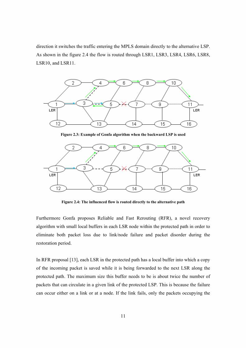
In the figure 2.3 the main path is established between LSR1, LSR3, LSR5, LSR7, LSR9
and LSR11 and the alternative path is established between LSR1, LSR2, LSR4, LSR6,
LSR8, LSR10 and LSR11. Also the backward LSP LSR3, LSR1 is established for the
SPD 1-3 and 1-2-4-3. The second backward LSP is LSR7, LSR5, LSR3 for the SPD 3-5-
7 and 3-4-6-8-7. The final backward LSP is LSR11, LSR9, LSR7 for the SPD 7-9-11 and
7-8-10-11. In case of fault between 5 and 7 the data flow is going to be routed at the
backward LSP LSR5, LSR3, LSR4 and then will be transferred to the alternative path
LSR4, LSR6, LSR8, LSR10, LSR11. When the LSR3 detects traffic in the reverse
11
direction it switches the traffic entering the MPLS domain directly to the alternative LSP.
As shown in the figure 2.4 the flow is routed through LSR1, LSR3, LSR4, LSR6, LSR8,
LSR10, and LSR11.
Figure 2.3: Example of Gonfa algorithm when the backward LSP is used
Figure 2.4: The influenced flow is routed directly to the alternative path
Furthermore Gonfa proposes Reliable and Fast Rerouting (RFR), a novel recovery
algorithm with small local buffers in each LSR node within the protected path in order to
eliminate both packet loss due to link/node failure and packet disorder during the
restoration period.
In RFR proposal [13], each LSR in the protected path has a local buffer into which a copy
of the incoming packet is saved while it is being forwarded to the next LSR along the
protected path. The maximum size this buffer needs to be is about twice the number of
packets that can circulate in a given link of the protected LSP. This is because the failure
can occur either on a link or at a node. If the link fails, only the packets occupying the

12
link from LSR5 to LSR7 during the failure would potentially be lost (Figure 2.4). If node
LSR7 fails, packets on two links will have to be recovered.
There are two possible modes to store the incoming protected packets to the local buffer.
The first, called the non-swapped mode, is to store the protected packets before the
swapping procedure to the backward/alternative LSP is done. This consists of a simple
copy of packets to the local buffer as the packets are received by an LSR. The second is
the swapped mode, in which the LSR stores the protected packets to the local buffer after
executing the swapping procedure to the backward/alternative LSP. Both modes work
well. The main differences between these approaches are the delay and the additional
process overhead.
When a fault is detected by an LSR, a switchover procedure is initiated immediately and
all the packets in its buffer are drained and sent back via the backward LSP. Any
subsequent packet coming in on the protected LSP is also sent back. The switchover
consists of a simple label swapping operation from the protected LSP to the backward
LSP. Note that this node has copies of packets that were dropped from the faulty
link/node and hence there is no packet loss.
As soon as each node of the backward LSP detects the first packet coming back, it
forwards this packet along the backward LSP and invalidates all data that are stored in its
buffer for recovery of data from a possible link/node failure associated with this output
interface. The next packet coming in from the upstream LSR of the protected LSP will be
tagged and forwarded to the downstream LSR via the protected LSP. All subsequent
packets that arrive at this node or LSR along the protected path are stored in its buffer
without being forwarded. This contributes significantly to the reduction of the average.
When a node detects the packet it tagged coming along the backward LSP, it knows that
all downstream packets have been drained and that it must now send back all its buffered
packets. By doing this, it is able to preserve the ordering of packets. Using one of the Exp
field bits of the MPLS label stack [25] for the purpose of tagging avoids any overheads.

13
Each LSR along the backward LSP successively sends back its stored packets when it
receives its tagged packet. Note that the node responsible for removing the tag is the
same node (LSR) which tagged it. When all packets return to the ingress LSR (i.e., the
ingress LSR receives its tagged packet) and have been rerouted to the alternative LSP, the
restoration period terminates. The packets stored during this time in the ingress LSR,
along with all new incoming packets (from the source) are now sent via the alternative
LSP. Note that at the end of the whole process, global ordering of packets is preserved,
packet loss has been eliminated.
Two Path Algorithm Two Path algorithm [5] [6] [74] uses protection switching mechanism with global
restoration of the MPLS network. Two alternative paths are created, in order to switch the
influenced data flow in case of any link failure. For each LSR two protections paths are
calculated and also the two protection paths may share links with the working path. All
paths protecting LSPs leading towards a common egress router are calculated
simultaneously using the algorithm. A full domain protection is achieved by a concurrent
execution of the protection path placement algorithm in each egress router. Finally it
assumed that the graph G(N,L) that represents the topology of the domain has edge
connectivity Ec(G)>2).
In the topology of the figure 2.5 the egress LSR is node A. Every node can be ingress
node of a data flow. Let assume that the node K is the ingress LSR and the working path
is between nodes Κ – J – I – E – D – A. Every node has two protection paths. The first
alternative path is established between K – F – G – H – C – B – A and the second
alternative path is established between Κ – J – I – E – D – A. After the link failure
between J and I the influenced flow is switched to the alternative path K – F – G – H – C
– B – A.

14
Figure 2.5: Example of Two path algorithm
Algorithm RBPC It is proven by that in a un-weighted network a reroute necessitated by any single link
failure can be obtained by concatenating at most two surviving shortest paths from the
original network. In general the theorem shows that concatenating at most k+1 such path
suffices to restore any route in the case of any k link failures. The algorithm Restoration
By Path Concatenation (RBPC) is based on this theory. The algorithm RBPC [1] uses as
a fact that in case of a failure, there is an alternative path which is the concatenation of at
most two original shortest paths. The restoration begins after finding the shortest paths
that when they are combined will shape the alternative path. RBPC uses the MPLS stack
mechanism to route packets along the concatenation of the basic paths. In the case of
finding two shortest LSPs to create the alternative path, the first label is used to transfer
the packets to through the first LSP and second label is used to transfer the packets via
the second LSP until they reach the egress LSR.
The algorithm gives the opportunity to use either global or local restoration, with the
combination of protection switching technique. When the local restoration is selected
then the upstream LSR is responsible to route the data flow around the failure by
concatenating already established paths. In the figure 2.6 the working path is between
LSR1, LSR3, LSR5, LSR7, LSR9 και LSR11. Also the LSP2 exists between LSR3,
LSR13 and LSR14, and LSP3 between LSR14, LSR15 and LSR16. The concatenation of
the LSP2 and LSP3 is the new shortest path between LSR3 and the egress LSR. When

15
the failure in LSR5 is detected from upstream LSR3, the packets are forwarded through
LSP2 and LSP3 using the MPLS stack mechanism.
Figure 2.6: Example of RBPC algorithm (local)
In the case of global restoration, when the upstream LSR detects the failure is responsible
to inform ingress LSR by sending FIS messages. Ingress LSR will switch the influenced
data flow using the concatenation of already established paths, as shown in the figure 2.7.
Figure 2.7: Example of RBPC algorithm (global)
Dual Algorithm Dual Algorithm [9] uses protection switching mechanism in combination with local
restoration. The working path and alternative paths are established simultaneously and
this is achieved with the modification of the LDP protocol. Specifically, additional
parameters are added to the optional parameters field of the label request message (LRM)
and the label mapping message (LMM) [4]. The LRM contains a successor LRM
(SLRM) and a feasible successor LRM (FSLRM), respectively. The SLRM is used to
request the label of working path according to the successor of routing table and FSLRM

16
is used to request label of backup path according to the feasible successor of routing
table. The LMM contains the successor LMM and the feasible successor LMM, which
are used to map label of working path and backup path, respectively. In addition the
Label Information Base (LIB) [4] is modified to add an additional state field to record
which label is assigned to working path or backup path.
The initial topology is the network to the left of figure 2.8. When Dual algorithm is
applied the working LSP is established between S – A – E – C – D. While simultaneously
the local LSP S – Η – E, Α – Β – C and E – F – D are established. If a fault occurs
between A – E, then the upstream LSR forwards the packets through Α – Β – C.
Figure 2.8: Example of Dual algorithm
MBAK algorithm This algorithm uses protection switching mechanism with global restoration of the MPLS
network. The concatenation of paths is the basic idea of the MBAK algorithm [24] in
order to calculate the global alternative path. MBAK algorithm is developed to calculate
appropriate alternate paths in an undirected graph for a node pair (s, t). Specifically, for
each packet to be sent from s to t, this algorithm randomly chooses an intermediate node
e from a selected set of network nodes. Node e is called the pivot node. The packet will
be routed to t along a shortest path from s to e, and then routed along a shortest path from
e to t. The alternative paths are calculated using the same idea, by having as a pivot
another node in the undirected graph, apart from node e. After finding all possible path,
the two most acceptable alternative paths are going to be selected based on predetermine
constraints.
The pseudo code of MBAK for a graph G(V, E) is:
17
1. Construct the shortest path tree (SPT) rooted at the source node s, and the SPT rooted at the destination node t.
2. Obtain the shortest path (the primary path) from s to t, say P0(s, t). 3. Put each node x ε [V – all nodes on P0(s, t)] into a node set T. We call T the set of
pivot nodes, which contains all nodes of G that are not on P0(s, t). 4. For each x ε T, construct a path P’(s, t) = P0(s, x) + P0(x, t). Put P’(s, t) into a path set
H. If P’(s, t) contains a loop, or P’(s, t) is a duplicate path in H, then we do not put P’(s, t) into H.
5. Sort the path set H in ascending order according to the path length (the 1
st key) and
the shared edges between the primary and the related alternate path (the 2nd
key). 6. Choose two acceptable alternate paths from H by considering the pre-defined
constraints for path lengths and the number of shared edges.
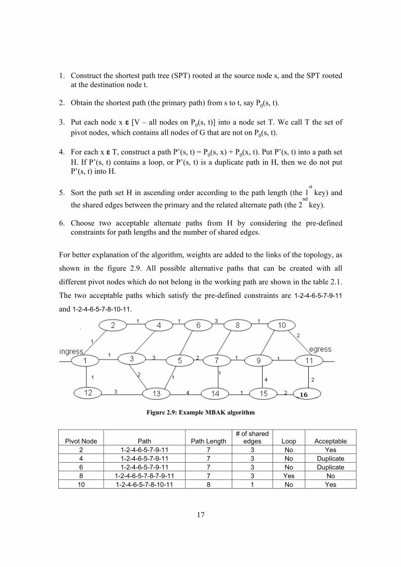
For better explanation of the algorithm, weights are added to the links of the topology, as
shown in the figure 2.9. All possible alternative paths that can be created with all
different pivot nodes which do not belong in the working path are shown in the table 2.1.
The two acceptable paths which satisfy the pre-defined constraints are 1-2-4-6-5-7-9-11
and 1-2-4-6-5-7-8-10-11.
Figure 2.9: Example MBAK algorithm
Pivot Node Path Path Length # of shared
edges Loop Acceptable 2 1-2-4-6-5-7-9-11 7 3 No Yes 4 1-2-4-6-5-7-9-11 7 3 No Duplicate 6 1-2-4-6-5-7-9-11 7 3 No Duplicate 8 1-2-4-6-5-7-8-7-9-11 7 3 Yes No 10 1-2-4-6-5-7-8-10-11 8 1 No Yes
18
12 1-12-13-5-7-9-11 9 3 No Yes 13 1-3-13-5-7-9-11 8 4 No Yes 14 1-2-4-6-5-7-14-7-9-11 8 3 Yes No 15 1-2-4-6-5-7-14-15-16-11 11 1 No Yes 16 1-2-4-6-5-7-14-15-16-11 11 1 No Duplicate
Table 2.1: All possible alterative paths of MBAK algorithm
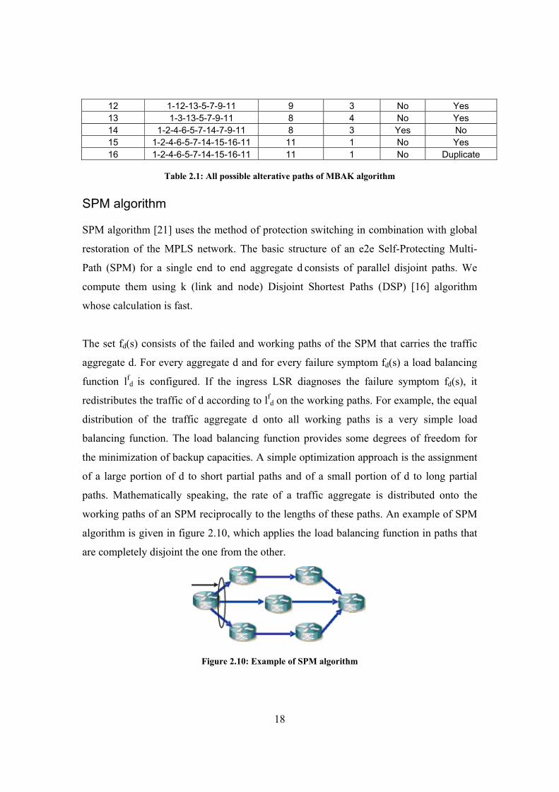
SPM algorithm SPM algorithm [21] uses the method of protection switching in combination with global
restoration of the MPLS network. The basic structure of an e2e Self-Protecting Multi-
Path (SPM) for a single end to end aggregate d consists of parallel disjoint paths. We
compute them using k (link and node) Disjoint Shortest Paths (_DSP) [16] algorithm
whose calculation is fast.
The set fd(s) consists of the failed and working paths of the SPM that carries the traffic
aggregate d. For every aggregate d and for every failure symptom fd(s) a load balancing
function lfd is configured. If the ingress LSR diagnoses the failure symptom fd(s), it
redistributes the traffic of d according to lfd on the working paths. For example, the equal
distribution of the traffic aggregate d onto all working paths is a very simple load
balancing function. The load balancing function provides some degrees of freedom for
the minimization of backup capacities. A simple optimization approach is the assignment
of a large portion of d to short partial paths and of a small portion of d to long partial
paths. Mathematically speaking, the rate of a traffic aggregate is distributed onto the
working paths of an SPM reciprocally to the lengths of these paths. An example of SPM
algorithm is given in figure 2.10, which applies the load balancing function in paths that
are completely disjoint the one from the other.
Figure 2.10: Example of SPM algorithm

19
2.1.2 Rerouting algorithms Dynamic Routing algorithm Dynamic routing algorithm [13] employs rerouting technique in combination with global
recovery of the network. When the upstream LSR detects a failure, then immediately
sends FIS messages to the ingress LSR. After receiving the FIS messages the ingress
LSR calculates dynamically and establishes the new alternative path that will route the
influenced flow. Finally, the packets are routed through the new path. This algorithm is a
modification of the Makam’s proposal.
When the failure of LSR5 is detected by LSR3, LSR3 sends FIS messages to inform the
ingress LSR about the failure. The ingress LSR calculates the new path which is LSR1,
LSR2, LSR4, LSR6, LSR8, LSR10 and LSR11, as shown in the figure 2.11. After
establishing the path, the ingress LSR switches the flow to the new path.
Figure 2.11: Example of Dynamic Routing Algorithm
A.J.C Algorithm The proposal of A.J.C [2] is based on rerouting mechanism and recovers the failure
locally. The algorithm uses the following steps in order to recover from a failure:
1. The upstream LSR that has detected a failure calculates the least-cost path of all possible alternative paths between itself and each Candidate-PML. Candidate-PML is an LSR on working path that can be used as PML (Protection Merging LSR). As the result, the upstream LSR can know the PML of the least-cost path and the explicit route up to the PML.
2. A recovery path is established along the calculated explicit route from the upstream
LSR to the PML. In the recovery path setup, the explicit route is inserted into the ER

20
(Explicit Route) of MPLS signaling message (e.g., CR-LDP, RSVP). And LSPID (LSP Identifier) of the working LSP is used as an ER hop for the purpose of splicing the existing working LSP and its new recovery LSP to be established. The holding priority of the working path may be used as the setup priority of the recovery path.
3. As soon as the recovery path is established, traffic on the working path is switched
over to the recovery path. 4. If the setup of the recovery path fails, go to 1.
In the topology shown in figure 2.12 the working LSP is LSR1, LSR3, LSR5, LSR7,
LSR9 and LSR11. When the fault is detected by LSR3, and then is responsible to
calculate the least-cost path. In this case the least-cost path is the path with the smallest
number of nodes between LS3 and candidate PML, which is the path between LSR3,
LSR13, LSR14 and LSR7. As soon as the recovery path is established, traffic on the
working path is switched over to the recovery path.
Figure 2.12: Example of A.J.C algorithm
Yoon Algorithm
Yoon [2] [27] suggests an efficient pre-qualified recovery mechanism, which optimizes
the network performance by considering link usage. Since an existing recovery
mechanism, pre-qualified rerouting, selects a backup path only once at the LSP setup
time, it may not reflect the exact status of network resources at the time of a fault. In
contrast, this approach exchanges network status information among LSRs so that the
backup path selection engine can use up-to-date information and decide an optimal
backup path for a possible failure. The new proposed recovery mechanism can always

21
maintain an optimized network state regardless of the fault occurrence. The upstream
LSR can choose an optimal path up to its downstream LSR by re-calculating the path
whenever network status is changed. When a link failure occurs, the upstream LSR that
has detected it establishes a recovery path along the pre-calculated optimal path.
The working LSP in this topology is LSR1, LSR3, LSR5, LSR7, LSR9 and LSR11, and
the path between LSR3, LSR13, LSR14, and LSR7 is pre-calculated but not established.
When the fault occurs LSR3 is going to establish the alternative local path and switch the
data flow to the alternative path, as shown in figure 2.13.
Figure 2.13: Example of Yoon Algorithm
Chen & Oh Algorithm The next algorithm uses rerouting mechanism in combination with local restoration of the
network. Chen and Oh [2] [10] have proposed a scheme, in which recovery paths are pre-
established between links on working path without reserving resources. When a link
failure occurs, the downstream LSR that has detected it sends a notification message
(e.g., CR-LDP notification message) to its upstream LSR to check and reserve resources
and to notify to the upstream LSR. The advantage of this proposal is the better utilization
of the resources.
The working LSP in this topology is LSR1, LSR3, LSR5, LSR7, LSR9 and LSR11, and
the path between LSR3, LSR13, LSR14, and LSR7 is pre-calculated and established,
without reserving any resources. When the fault occurs LSR7 will send FIS message to

22
the upstream LSR, while simultaneously resources are reserved. Finally LSR is going to
switch the data flow to the alternative path, as shown in figure 2.14.
Figure 2.14: Example of Chen & Oh Proposal
Otel Algorithm Now we will examine the Otel algorithm which uses local repair and rerouting
techniques. The algorithm uses three data structures [22].
1. The Shortest Path Tree (SPT) where the root is the node that will execute the
calculations.
2. An array of lengths which contains the length of the shortest path between the
SPT root and to all other nodes.
3. A priority queue for nodes. In this queue all nodes are represented as quadruples
of the form (n, p, ∆, l) where n is for the node, the ∆ is the quadruple key, p is the
tentative of the parent for n in the SPT and l the network link directed from p to n.
The priority queue operates as follows:
• Whenever a new quadruple for node n is inserted in the queue, the insertion
operation checks whether the queue already contains a quadruple for node n.
If yes, the existing quadruple is replaced by the new one only if the key in the
new quadruple is smaller than the key in the quadruple already enqueued.
• Whenever an element is to be extracted from the queue, the quadruple with
the minimum ∆ is chosen and removed from the queue. If there are several
such elements the length of the tentative path for the quadruple is used as a
tie-breaker, with the quadruple having the shortest tentative path length being

23
consider first. For a quadruple the tentative path length is computed as the
shortest path length from the SPT root to node p plus the weight of the link.
These are the steps that Otel algorithm follows [22]:
Step 1: Mark all the nodes in the existing SPT as “reachable”. Step 2: Consider the SPT subtree rooted at the disconnected downstream LSR. Starting with the subtree root, mark all the nodes in this subtree as “unreachable”. Step 3: Construct L, the set of the network links in the residual topology that have as ingress a reachable node and as egress an unreachable node. Step 4: For each link l in the set of L:
• Consider p and n, the nodes at the ingress and, respectively, egress of link l. Compute the length of the tentative path from the SPT root to the node n as the length of the shortest path to the reachable node at the ingress of the link l (node p) plus the weight of the link l .
• Compute ∆ as the difference between this path length and the length of the shortest path between SPT root and node n in the old outdated topology.
• For node n insert in the priority queue the quadruple formed by these values of n, p, ∆ and l .
Step 5: From the priority queue extract one quadruple, (n’, p’, ∆’, l� ).Update the SPT by deleting the branch linking n’ with its parent in the old SPT and adding as an SPT branch the link l’, connecting unreachable node n’ with its reachable parent, node p’. Also update the array of shortest path length by computing the shortest path length from SPT root to node n’ as being the length of the shortest path to node p’ plus the weight of the link l �. If the node n’ is the destination node the algorithm is terminated. Step 6: Mark n’ and all its descendents in the SPT as reachable. Remove from priority queue all quadruples corresponding to all these descendants. Reset the value for the link set L as consisting of all the links that have as ingress node n’ or any of its descendants and as egress an unreachable node. Go to step 4.
Below is an example with Otel algorithm to be responsible for the recovery of the
network. In the figure 2.15 there is a fault in the main path between 5 and 7. Firstly the
SPT is created where the root is the LSR 5 because this is the upstream LSR which
detects the fault and also the array of lengths. These structures are given at the figure
2.16(a) and 2.16(b) respectively.

24
Figure 2.15: A fault occurs between 5 and 7
Figure 2.16: (a) The SPT with the LSR 5 being the root. (β) The array of lengths
For the 2nd step we mark the nodes are unreachable, these are 7, 9, 11. Then in the 3rd step
we create the set L which contains the links 8-7, 14-7, 10-9, 15-9, 10-11 and 16-11. In the
4th step for every link we create a quadruple (n, p, ∆, L.) as shown in table 2.2. Then we
insert the quadruples with the smallest ∆ for every unreachable node in the priority
queue. Consequently the quadruples that will be inserted are 7–14, 9–15 and 11–10.
n ∆ p l 7 2 8 7 – 8 7 2 14 7 – 14 9 2 10 9 – 10 9 2 15 9 – 15

25
11 1 10 11 – 10 11 2 16 11 – 16
Table 2.2: The quadruples that are created at step 4
At the 5th step we select the quadruple with the smallest ∆ which is the quadruple of node
11 and extract it from the priority queue. Then the SPT is informed connecting the branch
of node 11 to the node 10. The node 11 is the destination node and the algorithm is
terminated. At the figure 2.17(a) is the SPT after the fault and at the figure 2.17 (b) is the
array of lengths. From the SPT we derive the alternative path which is 5-6-8-10-11 and
we establish it. This is shown at figure 2.18.
Figure 2.17: (a) The SPT after the fault. (b) The array of lengths after the update.
Figure 2.18: The influenced data flow is routed through the local alternative path

26
MIRA Algorithm This algorithm uses rerouting technique and finds a global alternative path to restore the
traffic. The key idea of MIRA [17] [8] is to route an incoming connection over a path
which least interferes with possible future requests. The algorithm is based on the theory
of maxflow and tries to maximize the capacity between the ingress and egress node,
improving the probabilities for finding of alternative paths when failure occurs.
INPUT: A graph G(N,L) and a set B of all residual link capacities. An ingress node a and an egress node b between which a flow of D units have to routed.
OUTPUT: A route between a and b having a capacity of units of bandwidth. ALGORITHM: 1. Compute the maximum flow values for all (s,d) ε \P(a,b) 2. Compute the set of critical links Csd for all (s,d) ε \P(a,b) 3. Compute the weights w(L) = S (s,d):l ε Csd αsd V L ε L 4. Eliminate all the links which have residual bandwidth less than D and form a reduced
network. 5. Using Dijkstra’s algorithm compute shortest path in reduced network using w(L) as
the weight on link L. 6. Route the demand of D units from a to b along this shortest path and update the
residual capacities.
With the topology shown in figure 2.19, MIRA algorithm is going to be explained. There
are three potential source destination pairs, (S1,D1), (S2,D2), (S3,D3). Assume that all
links have a residual bandwidth of 1 unit and there are three different data flows with the
following order S3,D3,1), (S2,D2,1), (S1,D1,1). The ling between node 7-8 is considered
to be critical path for (S1, D1), (S2, D2) pairs. When (S3,D3,1) data flow is going to be
routed, MIRA algorithm tries to avoid critical links and routes the flow through the path
1-2-3-4-5.

27
Figure 2.19: Example of MIRA algorithm
Hong’s Algorithm Hong’s proposal [15] is based on rerouting technique and repairs the failure locally. One
of the requirements of the algorithm is an Intermediate Weighted Network Graph
(IWNG). After detecting the fault, an intermediate ingress node I’ is determined which
belongs to the working path and is the upstream LSR from the failure point. Afterwards
the optimal alternative path is calculated from the I’ node to the egress LSR, based on
some restrictions like bandwidth. If the algorithm calculates the optimal path, then it is
selected and established in order to route the flow around the failure. Otherwise, the
process is repeated but this time with a different intermediate ingress node I’.
Step 1: First, we create an Intermediate Weighted Network Graph (IWNG) with such information as F, LSPREQ(I,E, T,H,BREQ), and PWORKING. The weight (W) of IWNG is assigned by the IWNG creation algorithm. Step 2: We determine intermediate ingress node (I’) to generate an alternative LSP, that is to say, we confine the restoration scope that will be the most reasonable boundary to create an alternative path for the restoration of the occurred faults. In other words, we create LSPREQ(I’,E, T,H,BREQ). The I’ should be one of the nodes in PWORKING. Step 3: We find the most optimal alternative path from LSPREQ (I’) to LSPREQ (E) with the routing constraints such as T , H, and BREQ.. Step 4: If the path computation algorithm generates an optimal path between LSPREQ (I’) and LSPREQ (E), we select it as an alternative path (PREROUTING) for the restoration of the fault and stop the procedure.

28
Step 5: However, if there is no any reasonable alternative path between LSPREQ (I’) and LSPREQ (E), we compare the original ingress node (I) with I’. If I is the same node as I’, we stop the procedure because there can be no more wide restoration scope Step 6: If I is not the same node as I’, we define I’ as an implicit abnormal node (F ← LSPREQ(I’)), which results in the extension of restoration scope. As I’ is newly added to F, we iterate the above procedure from Step 1 until we find an optimal alternative path for restoration (Step 4) or there is no alternative path (Step 5). In figure 2.20 is an example of WNG graph where fault occurs in link L19. The working
path is established between a-L1-d-L8-h-L19-l. In figure 2.21, h node is becoming the
intermediate ingress node I’ and the alternative path is found through i,j.
Figure 2.20: Failure is detected in L19 link
Figure 2.21: Recovery from the failure of link L19
Lin & Lui Algorithm
This algorithm uses rerouting technique with global restoration of the failure. First, the
two edges LSR of each failure-free LSP are used in the simple graph as the ingress and
egress nodes. Between each ingress-egress node pair, an edge is set to connect them. The
cost and capacity in the edge are set to be the delivery delay and residual bandwidth of its
corresponding failure-free LSP. Between the source node and each ingress node and the
destination node and each egress node, there is also an edge to connect them, which

29
corresponds to a transmission path of the IP destination access network. The capacity of
each such edge is set to infinity and the cost of such each edge is set to the number of
transit hops in its corresponding transmission path. Figure 2.22 shows the modeling of a
simple graph [19].
Figure 2.22: Creation of the graph
Given the simple graph with an input traffic flow, the affected traffic distribution is
transferred to the problem how to send the traffic flow from the source node to the
destination node with a minimum cost (the minimum cost flow problem). Based on the
minimum cost flow problem can use the following linear equation to represent it:
where xk represents what amount of the affected traffic is redirected to failure-free LSPk, ck is the unit cost of a packet carried by failure-free LSPk, rk is the residual bandwidth of
failure-free LSPk, bLSP f is the bandwidth requirement of the affected traffic, n is the
number of failure-free LSPs.
After finding the alternative path, the packets are routed via the new path by using the
header encapsulation and decapsulation techniques, as shown in figure 2.23.

30
Figure 2.23: MPLS stack mechanism
2.2 Comparison of Existing MPLS recovery algorithms
Several criteria to compare the performance between different MPLS-based recovery
schemes are defined in [26]. These are: packet loss, additive latency, re-ordering,
recovery time, full restoration time, vulnerability, and quality of protection. Fault
recovery time is the time elapsed between the fault detection and the time when the first
packets are rerouted using the alternative path. Recovery time includes additive latency
and sometimes is the equivalent to full restoration time. Packet loss is the percentage of
packets lost until the fault is recovered. Packet reordering is whether the packets
delivered during the recovery period are delivered out-of-order or not. Vulnerability is
the time that the protected LSP is left unprotected and quality of protection is the
probability of a connection to survive the failure.
For the purposes of our work, which focuses more on the global performance and fault-
tolerance of the MPLS network, we consider the first three criteria (recovery time, packet
loss and packet disordering) and instead of vulnerability and quality of protection, we
consider, as a more suitable fourth criterion, the ability of the network to tolerate multiple
faults. For every performance criteria three algorithms are selected for each technique.
.

31
2.2.1 Fault Recovery time
Firstly the recovery time is the time elapsed between the fault detection and the time
when the first packets are rerouted using the alternative path (i.e. when the fault is
recovered). During the recovery time, packet routing is not paused so upstream LSR
continues to receive packets. In addition to this upstream LSR can not forward the
packets to the next LSR, since fault is detected, and the packets are dropped.
Consequently recovery time must be small in order to have low packet loss, especially if
we are dealing a real time application. Real time applications are very sensitive to packet
loss and when this happens the user might terminate the application. For this reason fault
recovery time is considered to be one of the most important criteria to evaluate an MPLS
recovery algorithm.
In general, if protection switching is used with global restoration, then the recovery delay
is the time until the FIS messages reach the ingress LSR plus the time needed for the
ingress LSR to decide which alternative path is best to use (when two or more alternative
paths exists) plus the time needed to switch the path and forward the packets to the
alternative LSP. When the local restoration is used, then the recovery delay is only the
time needed for the upstream LSR to decide which alternative path is best to use plus the
time needed to switch the path and forward the packets to the alternative LSP.
Consequently, the local repair needs less time to recover from failure than in global
repair. As a result the three best algorithms which are using protection switching are
Gonfa, Dual and Haskin where the alternative paths are established locally.
As for the algorithms which are using rerouting technique in order to recover from a fault
there are two cases as well. In the case of global restoration the recovery delay is the time
until the FIS messages reach the ingress LSR, plus the time needed to calculate and
establish the alternative path and the time to start forwarding packets to alternative path.
When local restoration is used, the recovery delay is the same as the global restoration
excluding the time needed for the FIS messages to be reach ingress LSR. However to be
32
able to select the tree bests algorithms with rerouting technique, it is required to examine
the complexity time of the algorithm that is used to calculate the alternative path.
One of the three best rerouting algorithms is the Yoon et al proposal, where the
alternative path is not calculated after the detection of the fault but during the setup time
of the working LSP. Consequently, the recovery time is minimized significantly because
of the pre-qualified recovery mechanism. The recovery time of this algorithm is the
establishment of alternative pre-qualified LSP plus the time needed to switch the packets
into the alternative path.
The next algorithm consider to have small recovery time is Chen & Oh algorithm. After
the detection of the failure there is no calculation of the alternative path due to the fact
that the alternative path is already selected and the only procedure needed is to reserve
the sources while establishing the path. This mechanism minimizes the recovery time and
makes this proposal on of the best algorithms in this performance criterion.
Finally, the Otel algorithm is selected among the algorithms which have short recovery
time. This algorithm calculates the alternative path after the detection of the failure. The
algorithm that is used to find the alternative path uses a lightweight incremental Dijkstra
algorithm which is optimized for computing a single pair shortest paths in a network
based on an incremental change in the topology and a SPT for the topology previous to
the change. Consequently, the SPT is calculated only once and this minimizes the
recovery time for each failure [22]. Also the complexity of the algorithm is dependent on
two interrelated factors:
1. The size of the SPT subtree affected by the failure
2. The number of links originating from nodes outside the subtree but incident to
subtree nodes.
Based on the given simulation results, two parameters influence the calculation of
alternative path base on logarithmic and linear complexity respectively [22]. As a result
this algorithm is included in one of the best algorithms for this criterion when is

33
compared with the rest of the algorithms which calculate the alternative path
dynamically.
2.2.2 Packet Loss In the time interval between detection of fault in the network and switch over of
influenced data flow to the alternative path packets loss is observed. The loss of packets
influences significantly the throughput rate. In real time applications such as video
streaming the packet loss may force the user to terminate the connection. For this reason
the fault have to be repaired with the minimum packet loss. Packet loss is a basic
criterion to compare prior work for fault tolerance in MPLS. The packet loss is
proportional to the recovery time. When the time needed to recover from the failure is
long then many packets are going to be lost. Thus, the determination of the three best
algorithms for this criterion is based on the fault recovery time of each algorithm.
The algorithms which employ protection switching technique and have better results on
packet loss are the algorithms with local restoration. As soon as the upstream LSR detects
the failure, instantly routes the packets into the alternative path. This technique will not
cause a major delay, therefore no significant packet loss. As a result the three best
protection switching algorithms are Gonfa, Dual and Haskin where there alternative paths
are pre-established locally and immediately after detection of a fault, the flow is routed to
the alternative path.
The algorithms employing rerouting technique and have good results for packet loss are
the algorithms with short recovery time. For this reason Yoon, Chen & Oh and Otel
algorithms are considered to be the three best rerouting algorithms for this criterion. The
first two have are expected to have better results because the packet loss will occur until
the pre-qualified alternative paths are established. In the case of the Otel algorithm the
packet loss expected to be observed will be larger than the previous two algorithms but
smaller than the rest of rerouting algorithms. This is because Otel algorithm has better
fault recovery time than the rest of rerouting algorithms.

34
2.2.3 Packet Reordering Furthermore the recovery of the network can cause reordering of packets. The cases
where reordering packets is caused is when the delay of the existing path between two
nodes is greater than the delay of the alternative path for those two nodes. This is the case
for the local repair. The second case is when the delay until the FIS is received by the
ingress LSR with the delay of the alternative path is smaller than the delay of the existing
path. This is the case for the global repair. Also reordering may introduced when packets
arriving from the reverse direction are mixed with incoming packets, this results in packet
disordering through the alternative LSP during the restoration period. This is also not
desirable. While data transfers may handle disordered packets, streaming data usually do
not. That is why packet reordering is considered to be one of the most important criteria
to compare related work of fault tolerant algorithms.
The first protection switching algorithm considered to be one of the best which avoids
reordering is Makam’s algorithm. There is no use of backward LSP, so the incoming
packets are not mixed up with the packets coming from backward LSP. Also the time
interval between FIS messages to arrive at the ingress LSR and the packets to reach
destination is longer than the time required for packets which successful arrive at the
downstream LSR just before failure to reach the destination. For the same reasons, RBPC
algorithm with global restoration achieves to be one of the best algorithms in this
criterion. The next algorithm with small packet reordering is Gonfa, due to the fact that is
using RFR proposal. With RFR packet disordering during the restoration period is
avoided.
As for rerouting algorithms, Lin and Lui, MIRA and A.J.C algorithms are selected for
this criterion. The first two algorithms are using global restoration, therefore the recovery
time plus time needed for the packets to be transferred via the alternative path and reach
the destination is longer than the time required for packets which successful arrive at the
downstream LSR just before failure to reach the destination. This is because in addition
to the calculation time of the alternative, the time required for the FIS message to reach
the ingress LSR is added. Finally A.J.C algorithm is selected, even though the restoration
35
is done locally. The main reason of choosing this algorithm is due to complexity time of
the algorithm which is used to calculate the alternative path. Specifically, the algorithm
calculates the least-cost path of all possible alternative paths between itself and each
Candidate-PML. So the calculation of the alternative path takes longer time the rest of the
rerouting algorithms and the disordering of packets is avoided.
2.2.4 Multiple Fault Tolerance In a MPLS network multiple faults can be detected in the existing path but also in
alternative. If the algorithm can not tolerate in such type faults, this means that valuable
time is lost in order to install another path. The worst situation is when the algorithm can
not tolerate faults in both working and alternative paths. In this situation packet lost is
observed until a fault in alternative or working path is repaired. In the case of real time
applications this is repulsive. Tolerance in multiple faults is the fourth selected criterion
for the comparison of the MPLS recovery algorithms.
In protection switching algorithms this criterion is difficult to be fulfilled. Usually
protection switching algorithms can only recover from faults that occur in working path
but not in alternative paths. The three algorithms that serve better this criterion is Two
Path, RBPC and MBAK. The main idea of those algorithms is to establish one or more
alternative path. Specifically Two Path algorithm establishes two alternative paths. So it
can tolerate faults in working path and in one of the alternative paths. The same idea is
followed in MBAK algorithm, where again two alternative paths are established. The
worst situation in those algorithms would be to detect faults in working and in both
alternative LSPs. Finally RBPC algorithm is able to recover from multiple faults even if
they occur in alternative paths. That is, because is based on the idea of forming an
alternative path by concatenating two or more pre-established paths, whenever a failure is
detected.
When rerouting technique is followed in an algorithm then the algorithm is able to
tolerate multiple faults even if they occur in alternative paths. If a failure is detected in
working or alternative path, then each algorithm is going to calculate an alternative path

36
to reroute the data flow. Therefore the three best rerouting algorithms can not be chosen
due to the fact that all of them can reroute the flow whenever a failure is detected. The
only exceptions are the algorithms Yoon and Chen & Oh. In the first case the alternative
path is pre-qualified and in the second case the alternative path is already established and
only thing missing is to reserve resources. Hence when the failure is detected in
alternative path a new alternative path can not be dynamically calculated.
2.2.5 Comparison Summary
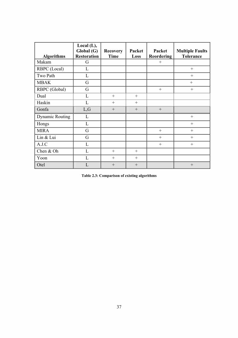
The characterization and evaluation of the existing fault tolerance algorithms based on
the selected criteria is shown in Table 2.3. The table is divided with two horizontal parts;
the upper level contains protection switching algorithms, whereas the lower level
contains rerouting algorithms. The symbol “+” indicates that the specific algorithm
satisfies adequately the corresponding criterion.
One can observe that the two algorithms which satisfy the most criteria are Gonfa [13]
and Otel [22]. The Gonfa algorithm is a protection switching algorithm which performs
well with respect to recovery time, packet loss and packet reordering criteria. On the
other hand, Otel algorithm is a rerouting algorithm which performs well with respect to
recovery time, packet loss and tolerance of multiple faults. In addition it can be observed
that the two algorithms are not able to satisfy all four criteria (only three each). Based on
these observations we decided to develop a new algorithm that makes use of these two
algorithms and is able to satisfy adequately all four criteria. The new algorithm is
presented in the next section.
37
Algorithms
Local (L), Global (G) Restoration
Recovery Time
Packet Loss
Packet Reordering
Multiple Faults Tolerance
Makam G + RBPC (Local) L + Two Path L + MBAK G + RBPC (Global) G + + Dual L + + Haskin L + + Gonfa L,G + + + Dynamic Routing L + Hongs L + MIRA G + + Lin & Lui G + + A.J.C L + + Chen & Oh L + + Yoon L + + Otel L + + +
Table 2.3: Comparison of existing algorithms

38
3 Hybrid Algorithm
To the best of our knowledge there is no current algorithm, either protection switching or
rerouting, able to perform well in all four criteria presented above. Motivated from this
observation we have developed a hybrid fault-tolerant algorithm that deploys effectively
both mechanisms based on the conditions of the fault, thus exploiting the advantages of
each one. The hybrid fault-tolerant algorithm is a combination of Gonfa protection
switching algorithm and Otel rerouting algorithm. The selection of these two algorithms
was based on the comparison of all algorithms on the four performance criteria.
Specifically, Gonfa algorithm is one of the best algorithms in recovery time, packet loss
and packet reordering criteria. Alternatively, Otel algorithm is one of the best algorithms
in recovery time, packet loss and multiple fault tolerance criteria
3.1 Fault Detection and Fault Notification The fault in a path can be detected using a link probing mechanism between neighbor
LSRs. An example of a probing mechanism is a liveness message that is exchanged
periodically along the working path between peer LSRs. For instance Keep Alive
messages can be used which are exchanged periodically between all neighboring routers
in the path. The LSR that detected the failure may be able to switch the flow to the
alternative path. If the node is not capable of initiating direct action (e.g., as a point of
repair, POR) the node should send out a notification of the fault by transmitting a FIS to
the POR. The FIS messages are transmitted with high priority so this ensures that FIS
will be propagated fast to the LSR which is in charge to restore the influenced flow [26].
3.2 Restoration and Notification LDP Hello Messages are exchanged periodically as part of the LDP Discovery
Mechanism. After the fault is repaired the hello messages are sent to its neighbours
indicating to them its presents. When the upstream LSR receives the hello messages,
realizes that the fault is repaired and notifies the POR node with Fault Recovery Signal
(FRS) messages. Restoration is performed upon receiving notification, via FRS

39
messages, that the working path is repaired, or upon receiving notification that a new
working path is established [26].
3.3 Algorithm Description The hybrid algorithm maintains four data structures: (i) a Shortest Path Tree (SPT) where
the root is the node that will execute the calculations, (ii) an array of lengths which
contains the length of the shortest paths between the SPT root and all other nodes, (iii) a
priority queue for nodes, (iv) a list maintained by ingress LSP and contains the working
and alternative LSP.
First, the establishment of the working LSP and the alternative LSP which protects the
whole working LSP is completed. Afterwards the segment protection domains are
determined along with their backward LSPs. Then the backward LSPs are established.
Also the alternative and backward LSPs are established based on the Gonfa algorithm.
The alternative LSP and backward LSPs are used by data flows with low priority. (When
a fault occurs, the LSPs will be needed for restoration of the fault. Hence the low priority
flows will stop routing via those paths in order to forward the influence data flow with
high priority). In addition, all the abovementioned data structures are created. Once the
initialization phase is complete, the algorithm begins its path maintenance operation
using the Gonfa algorithm. Depending on the nature and location of a fault as well as the
current state of the network topology, the algorithm might divert in using the Otel
algorithm and back (along with some additional calculations), as can be observed by the
Hybrid algorithm’s outline, given in next section. The data structure SPT is updated with
the use of any Single Source Shortest Part algorithm (SSSP) [18].
Next, we describe the two main cases of the hybrid fault tolerant algorithm, where based
on the outline the data flow is restored differently.

40
1st Case: Failures in working LSP followed by failures in alternative LSP
When a fault is detected in the working LSP and no other fault was detected previously in
alternative or backward LSPs, then the restoration of the MPLS network will be done
base on Gonfa algorithm. As long as the next faults occur in working LSP, Gonfa
algorithm will be used to repair the failure due to the fact that is capable to tolerate
multiple faults when these are located to working LSP.
Additionally FIS messages are send by upstream LSR to all other nodes to notify them
for the failure. Each node after receiving FIS messages, must update all the data
structures described in Otel algorithm. Thus, if Otel algorithm is needed to be applied in
order to repair a fault, all the data structures will be fully updated with the new state of
the network. The SPT can be updated by using single source shortest path algorithm
(SSSP).
If then a fault occurs in the alternative or backward LSPs, Gonfa algorithm will be no
longer capable of repairing the fault. Therefore, Otel algorithm is applied in order to
calculate an alternative path to restore the data flow. New faults may occur in the new
alternative path calculated by Otel algorithm; in this case again the Otel algorithm will be
responsible to find a new local path to switch the flow. This can be done as many times
as the times where failure is detected in alternative path because Otel algorithm can
tolerate multiple faults.
There is a modification of the Otel algorithm, where at the end of step 2 a condition is
added. The condition is to check if the destination node belongs to the reachable nodes. If
the condition becomes true then there is an alternative path and the algorithm is
temporarily stopped until the alternative path is established. Otherwise the algorithm
continues as it is. This modification is done to minimize the recovery time. After the
establishment of the alternative path, the flow is switched in the alternative path and
reaches the destination. In case of stopping at step 2, the algorithm now continues in
order to update all the structures and reflect the current state of the network.

41
2nd Case: Failures in alternative LSP followed by failures in working LSP
In case where the first fault is detected in alternative or backward LSP and no other fault
was detected previously in working LSP, the packets continue to be forwarded in
working LSP. Additionally FIS messages by upstream LSR to all other nodes to notify
them for the failure. Each node after receiving FIS messages, must update all the data
structures described in Otel algorithm. Thus, if Otel algorithm is needed to be applied in
order to repair a fault, all the data structures will be fully updated with the new state of
the network.
If a new fault occurs in working LSP then the restoration will be done base on Otel
algorithm. The reason is that the Gonfa algorithm is not able to be applied since the
alternative path can no longer be used. A rerouting technique must be followed in order
to repair the fault and that is why Otel algorithm is used. New faults may occur in the
new alternative path calculated in this case again the Otel algorithm will be responsible to
find a new local path to switch the flow.
In case of fault repair all the nodes update their SPT. The next step is to check whether
the working LSP is repaired by comparing the working LSP stored in the array and the
SPT. If the working LSP is repaired then the flow is switched back to the working LSP.
Otherwise, as next step is to check if the alternative LSP is repaired by comparing the
alternative LSP stored in the array and the SPT. If the alternative path is repaired then it
becomes available to route the flow when the working LSP becomes unavailable.
3.4 Outline of the algorithm
Figure 3.1 outlines the proposed algorithm.

42
Begin: Establish working, alternative and backward LSPs Compute:
1. SPT 2. Array of lengths 3. Array with the pre-established paths in Ingress LSR
Set _working_LSP as available Set _alternative_LSP as available Run the Gonfa algorithm Failure occurs check: If (failure is in working path)
Set _working_LSP as NOT available If (failure is in alternative path)
Set _alternative_LSP as NOT available If ( _working_LSP IS available && _alternative_LSP IS available)
Update SPT using SSSP and array of lengths If ( _working_LSP IS NOT available && _alternative_LSP IS available)
Step1: Recover from fault using the Gonfa algorithm Step2: Update SPT using SSSP and array of lengths
If ( _working_LSP IS available && _alternative_LSP IS NOT available) Update SPT using SSSP and array of lengths
If (_working_LSP IS NOT available && _alternative_LSP IS NOT available) Recover from fault using the Otel algorithm
When repair of a failure occurs check: Step1: Update SPT using SSSP and array of lengths Step2: Check: working LSP is repaired? If (compare array with pre-established paths in Ingress LSR and SPT)
Step1: Reroute the traffic in the working LSP Step2: Set _working_LSP as available
Else (compare array with alternative paths in Ingress LSR and SPT) Set _alternative_LSP as available
Figure 3.1: Outline of the Hybrid Algorithm
3.5 Example of Hybrid algorithm For a better understanding of the algorithm we describe a specific execution of the
algorithm and make use of the network topology given in Figure 3.2. The working path is
established between LSR1, LSR3, LSR5, LSR7, LSR9 and LSR11 and the alternative
path is established between LSR1, LSR2, LSR4, LSR6, LSR8, LSR10 and LSR11. The

43
first backward LSP is LSR3, LS1, the second backward is through LSR7, LSR5, LSR3
and the third backward LSP is formed by LSR11, LSR9 and LSR7.
The first link failure occurs between LSR5-LSR7 and base on Hybrid algorithm the
fault must be repaired using Gonfa algorithm. The data flow will be routed via the
backward LSP which it is formed by LSR5, LSR3 and then follow the alternative path
LSR4, LSR6, LSR8, LSR10 και LSR11. Afterwards the traffic will be routed directly to
the alternative path by LSR3, as shown in figure 3.3.
Figure 3.2: Route traffic via backward LSP
Figure 3.3: Route traffic directly into alternative path
The next step is to update all data structures of every node. In this example we are going
to concentrate on LSR3 because LSR3 is the upstream LSR of the next fault and will
become responsible to find the alternative LSP and route the flow. In figure 3.4 (a) the
SPT before the failure is shown and in figure 3.4 (b) SPT after the failure is shown.

44
Figure 3.4: (a)SPT before failure, (b) SPT after Failure
The next fault happens between LSR3-LSR4. Gonfa algorithm can not repair the fault,
only Otel algorithm is able to calculate an alternative path and route the data flow. The
SPT of LSR3 is shown in figure 3.4 (b). Hence the next step is to consider the SPT
subtree rooted at the disconnected downstream LSR and then starting with the subtree
root, all the nodes in this subtree are marked as “unreachable”. In this case the
unreachable node is only LSR4 and the destination node is a reachable node. Therefore
there is a path which can be used to route the data to the destination node. The local path
is LSR5, LSR6, LSR8, LSR10 and LSR11. Figure 3.5 shows how the data flow is routed
after the second failure.
Figure 3.5: Alternative path after 2nd failure

45
After routing the flow via the local alternative LSP, Otel algorithm continues in order to
update its data structures. Step 3 follows with the calculation of L set which consists links
between 2 – 4 και 6 – 4. In step 4 quadruples are created and for each node the quadruple
with smallest ∆ is inserted in the priority queue. In this case the quadruple with smallest
∆ is n=4, p = 2, ∆ = 2, and l = 2 – 4. In step 5 quadruple is extracted from the priority
queue and the SPT is updated by deleting the branch linking LSR4 and its parent LSR3
and adding as an SPT branch the linking LSR2 and LSR4, as shown in figure 3.6.
Figure 3.6: Updated SPT

46
4 Simulation and Analysis
4.1 Network Simulator 2 The methodology used for performance evaluation of the proposed hybrid algorithm is a
public domain network simulator version 2 (ns-2) originally from Lawrence Berkeley
National Laboratory (LBNL) [11] extended for MPLS networks called MPLS Network
Simulator (MNS) contributed by Gaeil and Woojik [12]. MSN supports basic MPLS
functions such as label switching, LDP, CR-LDP, and various options of label
distribution. The model has also functionality implemented for recovery mechanisms,
like the ability to setup a backup path and associate it with a working path.
The ns-2 is considered the standard simulation tool widely used by the network research
community to validate its new proposals. Therefore, the use of ns-2 as the evaluation tool
has many advantages.
1. It is a well proved standard network simulation with sufficient documentation.
2. It is maintained and updated by contributions from many people from different
network research groups.
3. The basic function and parameters in the simulator are calibrated properly. Therefore,
the simulation results derived from different proposals using the same simulation
conditions are feasible for evaluation. This allows easy and better comparison tools
between different proposals for network researchers.
Tool Command Language (TCL) [3] was used to create the different topologies and
scenarios and the developing of the three algorithms, Otel, Gonfa and Hybrid algorithm.
TCL is used for millions of people in the world. It is a language with a very simple
syntaxis and it allows a very easy integration with other languages. TCL was created by
Jhon Ousterhout.

47
4.2 Scenarios
We have performed simulations that experimentally evaluate and contrast the
performance (based on the four criteria) of the Hybrid algorithm with the performance of
Otel and Gonfa (i.e., the best representatives of each restoration mechanism). The
evaluation of the three algorithms was based on different scenarios. The network
topology along with the types and order of the faults were different in each simulated
case.
Different network topologies were used for the evaluation of the Hybrid, Otel and Gonfa
algorithms so as to examine their behavior in various types of topologies. Particularly, all
the network topologies used in the scenarios, are shown in figure 4.1. As it is observed,
the second topology represents a full mesh whereas the third topology is a circular
asterisk. The forth and fifth topology represents a communicational network of USA and
Great Britain, respectively. The characteristic of sixth topology is that there are many end
points. Topology number seven represents a hierarchical model while eighth topology is
a hierarchical model with bidirectional links. Finally ninth topology is a mesh topology.
The simulation results were analyzed by grouping the topologies in categories depending
on the number of nodes and links they have. We call a topology with a small number of
nodes (<10) as simple; otherwise we call it complex. Also, depending on the density of
the topology (small/large number of links) it is called sparse or dense (per the standard
graph-theoretic definitions). Hence, we have four different topology categories which are:
1. Simple and sparse topology includes first and seventh topologies.
2. Simple and dense topology includes fifth, sixth and ninth topologies.
3. Complex and sparse topology includes second and third topologies.
4. Complex and dense topology includes forth and eighth topologies

48
Figure 4.1: Network topologies
Furthermore the failure of links was another parameter examined in the simulations. In
general the following cases were examined:
1. The first fault to occur on the working path and then the second fault to occur on
the alternative path of Gonfa algorithm which is different from the Otel’s
alternative path.
2. The first fault to occur on the working path and then the second fault to occur on
the alternative path of Otel algorithm which is different from the Gonfa’s
alternative path.
3. The first fault to occur in working path and then node failure.

49
4. All faults to occur in working path.
5. The first fault to occur on the working path and then the second fault to occur in a
common link for the two alternative paths (Otel and Gonfa).
6. The first fault to occur on the working path and then the second fault to occur in a
common alternative path of Otel and Gonfa.
7. Random failures.
8. The first time to detect fault in the pre-established alternative path and then in the
working path.
In order to compare and evaluate the three algorithms the following results were taken for
each scenario. The results presented in each topology category are the average number
for a number of simulations where their topology belongs to the corresponding category
topology.
1. Received-Unordered-Lost packets: The results are shown through graph where x
axis represents the algorithms and y axis represents the number of packets.
2. Throughput - the amount of data transferred per second through links: The results
are shown through graph where x axis represents the time and y axis represents
Megabits per second.
3. Delays – time to receive packet: The results are shown through graph where y
axis represents the time and x axis to represents sequence number.
4. Recovery Time: The results are shown through graph where x axis represents the
algorithms with the faults and y axis represents the time in seconds.
4.3 Simple and sparse topology In the following figures the results received for the simple and sparse topology are
shown. In figure 4.2 measurements taken for the packet loss are shown. It is observed that
the Hybrid algorithm always gives the best results and is able to recover from all the
faults. Whereas Gonfa algorithm is unable to recover from faults which are detected in its
alternative path. Large amount of lost packets is observed in Otel algorithm when both of
faults are detected in the path used to route the flow. In figure 4.3 the number of disorder
packets is shown. In general the packet reordering is comparatively the same for the three
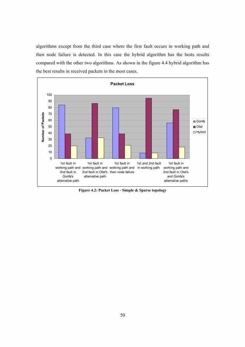
50
algorithms except from the third case where the first fault occurs in working path and
then node failure is detected. In this case the hybrid algorithm has the bests results
compared with the other two algorithms. As shown in the figure 4.4 hybrid algorithm has
the best results in received packets in the most cases.
Packet Loss
0
10
20
30
40
50
60
70
80
90
100
1st fault inworking path and
2nd fault inGonfa's
alternative path
1st fault inworking path and2nd fault in Otel'salternative path
1st fault inwotking path andthen node failure
1st and 2nd faultin working path
1st fault inworking path and2nd fault in Otel's
and Gonfa'salternative paths
Num
ber o
f Pac
kets
GonfaOtelHybrid
Figure 4.2: Packet Loss - Simple & Sparse topology
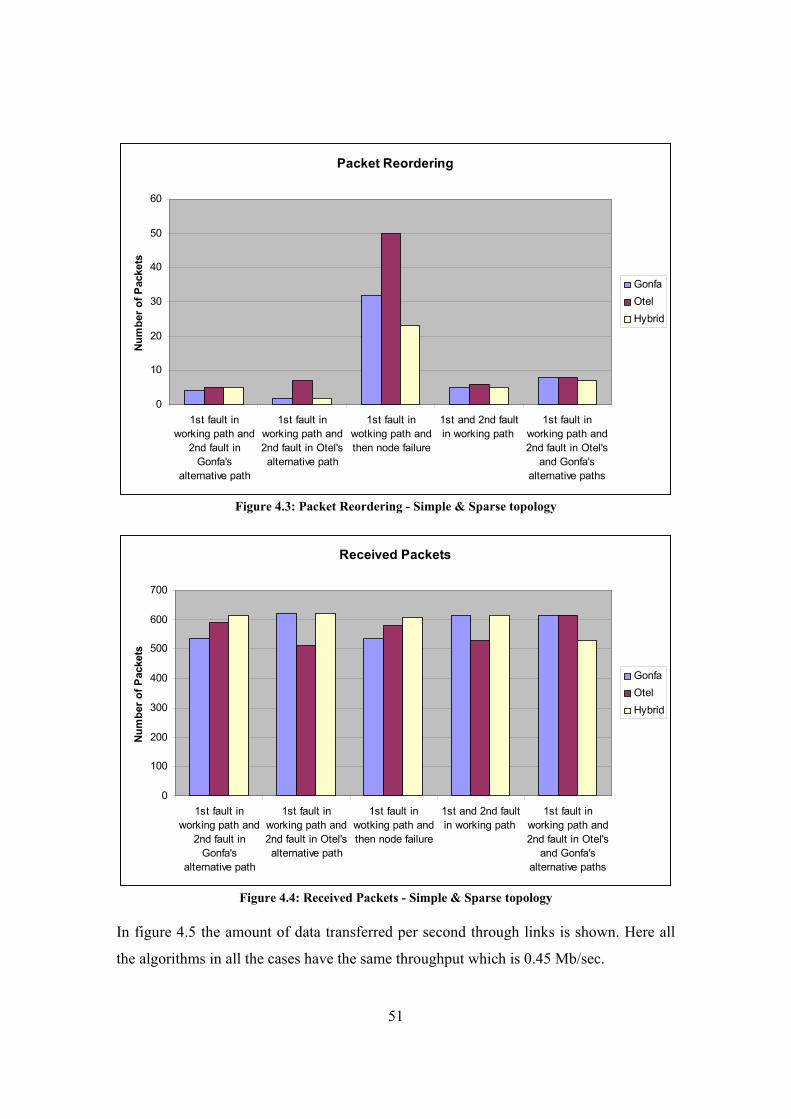
51
Packet Reordering
0
10
20
30
40
50
60
1st fault inworking path and
2nd fault inGonfa's
alternative path
1st fault inworking path and2nd fault in Otel'salternative path
1st fault inwotking path andthen node failure
1st and 2nd faultin working path
1st fault inworking path and2nd fault in Otel's
and Gonfa'salternative paths
Num
ber o
f Pac
kets
GonfaOtelHybrid
Figure 4.3: Packet Reordering - Simple & Sparse topology
Received Packets
0
100
200
300
400
500
600
700
1st fault inworking path and
2nd fault inGonfa's
alternative path
1st fault inworking path and2nd fault in Otel'salternative path
1st fault inwotking path andthen node failure
1st and 2nd faultin working path
1st fault inworking path and2nd fault in Otel's
and Gonfa'salternative paths
Num
ber o
f Pac
kets
GonfaOtelHybrid
Figure 4.4: Received Packets - Simple & Sparse topology
In figure 4.5 the amount of data transferred per second through links is shown. Here all
the algorithms in all the cases have the same throughput which is 0.45 Mb/sec.

52
Throughput
0
0.05
0.1
0.15
0.2
0.25
0.3
0.35
0.4
0.45
0.5
1st fault inworking path and
2nd fault inGonfa's
alternative path
1st fault inworking path and2nd fault in Otel'salternative path
1st fault inwotking path andthen node failure
1st and 2nd faultin working path
1st fault inworking path and2nd fault in Otel's
and Gonfa'salternative paths
Mb/
sec Gonfa
OtelHybrid
Figure 4.5: Throughput - Simple & Sparse topology
Now the results of the time needed to receive a packet are going to be displayed. The
delay time for each case of faults is shown.
1st fault in working path and 2nd fault in Gonfa's alternative path
Figure 4.6: Delay Time - Simple & Sparse topology

53
1st fault in working path and 2nd fault in Otel's alternative path
Figure 4.7: Delay Time - Simple & Sparse topology
1st fault in working path and then node failure
Figure 4.8: Delay Time - Simple & Sparse topology

54
1st and 2nd fault in working path
Figure 4.9: Delay Time - Simple & Sparse topology
1st fault in working path and 2nd fault in Otel's and Gonfa's alternative paths
Figure 4.10: Delay Time - Simple & Sparse topology
Recovery time is also measured in all the scenarios. Recovery time is the time interval
between detection of the failure and the time where the first packet is routed into the
alternative path. The figure 4.11 shows the recovery time needed for each algorithm to
restore a fault. When a fault do not influence the data flow, then the recovery time is set
to zero. Such case is when the fault occurs in Gonfa’s alternative path, Otel alternative
path is not the same as the Gonfa’s alternative path, therefore this failure does not
55
influence the data flow of Otel’s and there is no recovery time. Also there are faults that
Gonfa algorithm is not able to recover from them and the recovery time is again zero.
Such case is when the 1st fault occurs on working path and then on the alternative path, in
addition to this, the algorithm does not have another alternative path to reroute the flow
and is not able to recover from the last failure.
For the first case where the fault is detected in the working path and then in Gonfa’s
alternative path, it is observed that the three algorithms are able to recover from the first
failure. In the second failure Otel algorithm is not influenced and Hybrid algorithm is
able to find alternative path in 0,016 seconds. Gonfa algorithm has 0,02 recovery time
due to the fact that the working LSP is repaired and the flow is restored.
In the next case where the fault is detected in the working path and then in Otel’s
alternative path, it is observed that the three algorithms are able to reroute the flow into
an alternative path for the first fault. In the second failure Gonfa and Hybrid algorithms
are not influenced whereas Otel algorithm is able to find alternative path in 0,02 seconds.
The third case is when the 1st fault occurs in working path and then node failure is
detected. All the algorithms are able to recover from the first failure. As for the second
fault, Gonfa algorithm is not able to recover from it but due to the fact that the working
LSP is repaired and the flow is restored and the recovery time is set to 0,02. Otel and
Hybrid algorithms are able to find an alternative path in 0,02 and 0,012 sec respectively.
A difference between the recovery times for those two algorithms is noticed, this happens
because different SPTs are calculated for each algorithm. Hybrid algorithm uses SSSP
algorithm to update the SPT each time a fault occurs and does not affect the flow of the
data, hence different SPT is calculated from the SPT of the Otel algorithm.
As for the fourth case where all the faults occur in the working LSP, it is observed that all
the algorithms are able to recover from both failures. Gonfa algorithm can tolerate
multiple failures in the working LSP, that is why the first fault takes 0,0016 sec to
recover and the second fault takes 0,004 sec. The Hybrid algorithm in this case is

56
following the same procedures as the Gonfa algorithm. In the case of Otel algorithm, is
able to calculate an alternative path and reroute the traffic in both failures.
Finally, when the fault is detected in the working path and then in Otel’s and Gonfa’s
alternative paths, it is observed that all algorithms are able to restore the flow into an
alternative path for the first fault. However Gonfa algorithm is not able to recover from
the second fault and the recovery time is set to zero. Otel and Hybrid algorithm are able
to calculate dynamically the alternative path and switch the traffic in the alternative path
in 0,0012 seconds.
Recovery Time
0
0.005
0.01
0.015
0.02
0.025
1st fault inworking pathand 2nd fault
in Gonfa'salternative
path
1st fault inworking pathand 2nd fault
in Otel'salternative
path
1st fault inworking path
and then nodefailure
1st and 2ndfault in
working path
1st fault inworking pathand 2nd faultin Otel's and
Gonfa'salternative
paths
Tim
e
Gonfa - 1st failureGonfa - 2nd failureOtel - 1st failureOtel - 2nd failureHybrid - 1st failureHybrid - 2nd failure
Figure 4.11: Recovery Time - Simple & Sparse topology
4.4 Simple and dense topology
In the following figures the results received for the simple and dense topology are shown.
In figure 4.12 measurements taken for the packet loss are shown. There is not a case
where the hybrid algorithm has more packet loss than the other two algorithms. As
expected hybrid algorithm is able to recover from any failure. High packet loss is

57
observed in Gonfa algorithm when is unable to recover from failure in alternative LSP.
However Gonfa in fourth case where fault occurs in working path and then in a common
alternative path for Gonfa and Otel algorithm, low packet loss is noticed. The reason is
that Gonfa holds a buffer in each LSR and packets are stored there until fault is repaired,
in this way high packet loss is avoided. Also high packet loss is observed in Otel
algorithm when both faults affect the flow of the data and must find another alternative
LSP to recover from failure.
In figure 4.13 the number of disorder packets is shown. In the first two cases packet
reordering is approximately the same, but in the other two cases hybrid algorithm has
better results especially when is compared with Otel algorithm. Figure 4.14 show the
number of received packets, where hybrid algorithm has the best results in most cases.
Packet Loss
0
10
20
30
40
50
60
70
80
90
1st fault in workingpath and 2nd fault inGonfa's alternative
path
1st fault in workingpath and 2nd fault in
Otel's alternative path
1st fault in workingpath and then node
failure
1st fault in workingpath and 2nd fault inOtel's and Gonfa'salternative paths
Num
ber
of P
acke
ts
GonfaOtelHybrid
Figure 4.12: Packet loss - Simple & Dense topology
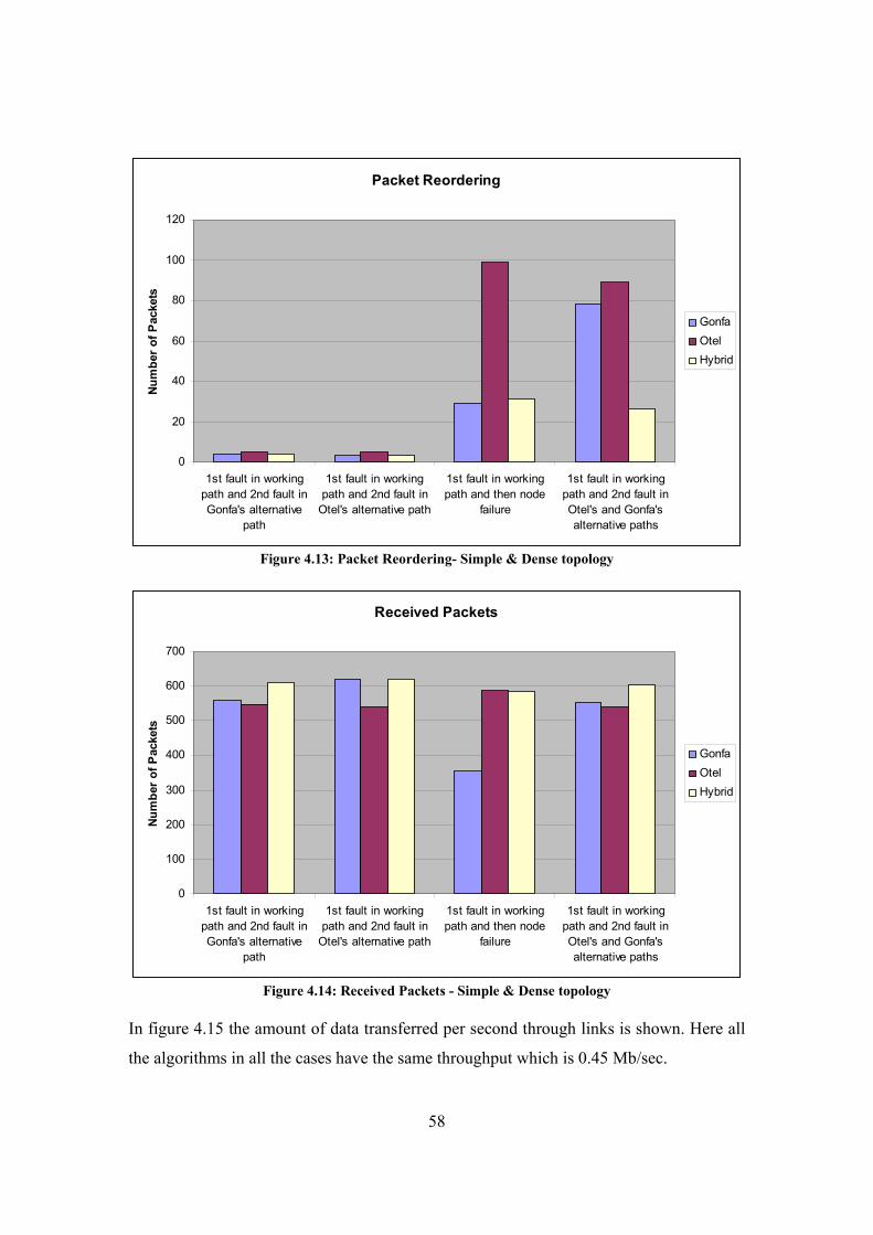
58
Packet Reordering
0
20
40
60
80
100
120
1st fault in workingpath and 2nd fault inGonfa's alternative
path
1st fault in workingpath and 2nd fault in
Otel's alternative path
1st fault in workingpath and then node
failure
1st fault in workingpath and 2nd fault inOtel's and Gonfa'salternative paths
Num
ber
of P
acke
ts
GonfaOtelHybrid
Figure 4.13: Packet Reordering- Simple & Dense topology
Received Packets
0
100
200
300
400
500
600
700
1st fault in workingpath and 2nd fault inGonfa's alternative
path
1st fault in workingpath and 2nd fault in
Otel's alternative path
1st fault in workingpath and then node
failure
1st fault in workingpath and 2nd fault inOtel's and Gonfa'salternative paths
Num
ber
of P
acke
ts
GonfaOtelHybrid
Figure 4.14: Received Packets - Simple & Dense topology
In figure 4.15 the amount of data transferred per second through links is shown. Here all
the algorithms in all the cases have the same throughput which is 0.45 Mb/sec.
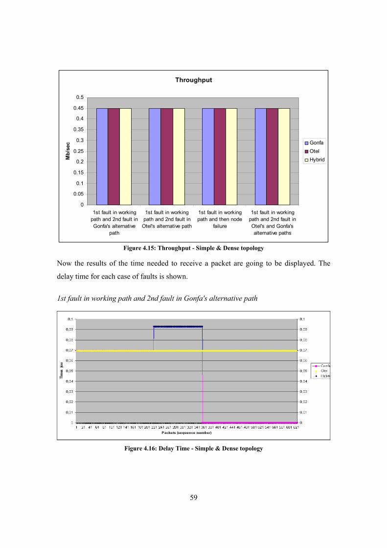
59
Throughput
0
0.05
0.1
0.15
0.2
0.25
0.3
0.35
0.4
0.45
0.5
1st fault in workingpath and 2nd fault inGonfa's alternative
path
1st fault in workingpath and 2nd fault in
Otel's alternative path
1st fault in workingpath and then node
failure
1st fault in workingpath and 2nd fault inOtel's and Gonfa'salternative paths
Mb/
sec Gonfa
OtelHybrid
Figure 4.15: Throughput - Simple & Dense topology
Now the results of the time needed to receive a packet are going to be displayed. The
delay time for each case of faults is shown.
1st fault in working path and 2nd fault in Gonfa's alternative path
Figure 4.16: Delay Time - Simple & Dense topology
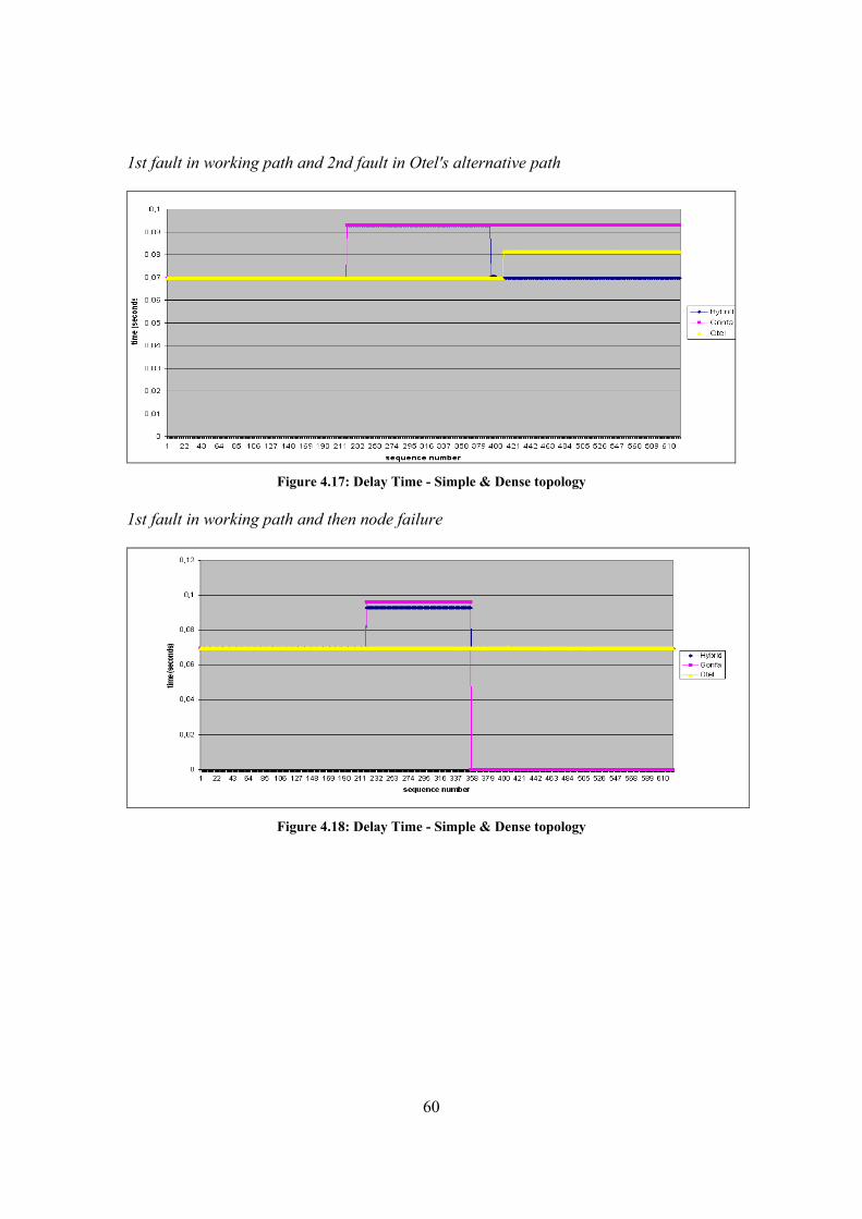
60
1st fault in working path and 2nd fault in Otel's alternative path
Figure 4.17: Delay Time - Simple & Dense topology
1st fault in working path and then node failure
Figure 4.18: Delay Time - Simple & Dense topology

61
1st fault in working path and 2nd fault in Otel's and Gonfa's alternative paths
Figure 4.19: Delay Time - Simple & Dense topology
The needed time to recover from a failure is shown in figure 4.20. As explained before
zero value can indicate either that flow of the specific algorithm is not influenced, or that
is not able to find an alternative path and reroute the failure. In the next scenarios, another
explanation is added to the zero value. This explanation refers to Otel algorithm, when
the working path is repaired in a certain time interval and the calculation of the alterative
path takes longer time than the certain time interval. Consequently, the flow is routed
immediately to the working path without waiting for the Otel algorithm to find an
alternative path.
For the first case where the fault is detected in the working path and then in Gonfa’s
alternative path, it is observed that the three algorithms are able to recover from the first
failure. In the second failure Otel algorithm is not influenced, so the recovery time is set
to zero. Gonfa algorithm has 0,0012 recovery time due to the fact that the working LSP is
repaired and the flow is restored. Hybrid algorithm has recovery time 0,0012 seconds.
These recovery times are the average number of the simulations where their topology
belonged to the simple and dense category. The fact that Gonfa and Hybrid algorithm
have the same recovery time can be explained either that the Hybrid algorithm was able
to restore the traffic into an alternative path in 0,0012 seconds or that during the

62
calculation of the alternative path, the working path was repaired and the flow was
immediately switched to working path.
In the next case where the fault is detected in the working path and then in Otel’s
alternative path, it is observed that the three algorithms are able to restore the affected
flow for the first fault. In the second failure Gonfa and Hybrid algorithms are not
influenced, so their recovery time is zero. As for Otel algorithm, is able to find an
alternative path and switch the traffic in 0,00147 seconds.
The third case is when the 1st fault occurs in working path and then node failure is
detected. All the algorithms are able to reroute the flow into an alternative path in the first
fault. As for the second fault, Gonfa algorithm is not able to recover from it and the
recovery time is set to zero. Otel algorithm is not affected from the node failure; therefore
the recovery time is set to zero. Hybrid algorithm is affected from the node failure and
needs 0,008 second to find an alternative path. The alternative paths for the two
algorithms are different because there SPTs are developed differently, so an error which
affects for example Otel’s alternative path does not imply that it will affect the Hybrid’s
alternative path.
Finally, when the fault is detected in the working path and then in a common alternative
path for the Otel and Gonfa algorithms, it is observed that all algorithms are able to
recover from the first failure with the same recovery time. However Gonfa algorithm is
not able to recover from the second fault and the recovery time is set to zero. Otel and
Hybrid algorithm are able to calculate dynamically the alternative path and switch the
traffic in the alternative path in 0,00105 and 0,0008 seconds, respectively. A difference
between the recovery times for those two algorithms is noticed, this happens because
different SPTs are calculated for each algorithm. Hybrid algorithm uses SSSP algorithm
to update the SPT each time a fault occurs and does not affect the flow of the data. In
each algorithm the SPT is developed differently and this obviously affects the calculation
time of the alternative path.

63
Recovery Time
0
0.0002
0.0004
0.0006
0.0008
0.001
0.0012
0.0014
0.0016
0.0018
1st fault inworking path and
2nd fault inGonfa's alternative
path
1st fault inworking path and2nd fault in Otel'salternative path
1st fault inworking path andthen node failure
1st fault inworking path and2nd fault in Otel's
and Gonfa'salternative paths
Tim
e
Gonfa - 1st failureGonfa - 2nd failureOtel - 1st failureOtel - 2nd failureHybrid - 1st failureHybrid - 2nd failure
Figure 4.20: Recovery Time
4.5 Complex and sparse topology In the following figures the results received for the complex and sparse topology are
shown. In figure 4.21 measurements taken for the packet loss are shown. In general
hybrid algorithm is able to recover from faults with minimum packet loss. In the 3rd case
hybrid algorithm has the highest packet lost from the other cases because all the links
connecting to the failed node can not be used. So there is a more than one link failure and
the SPT takes longer time to be updated. Gonfa algorithm is unable to recover from faults
which are detected in its alternative path. Also high packet loss is observed in Otel
algorithm when the fault occurs in the working and alternative path and must reroute the
traffic twice. Furthermore low packet loss is observed in Gonfa algorithm the fifth case
where the first fault happens in alternative LSP and then in working LSP. The reason is
due to the fact that Gonfa algorithm holds a buffer where the packets are stored in case of
a failure and also the second fault occurs in the end of the simulation.
In figure 4.22 the number of disorder packets is shown. In general the packet reordering
is approximately the same for the three algorithms except from the third case where node

64
failure is observed. As shown in the figure 4.23 hybrid algorithm has the best results in
received packets in all the cases.
Packet Loss
0
10
20
30
40
50
60
70
80
90
1st fault inworking path and
2nd fault inGonfa's
alternative path
1st fault inworking path and2nd fault in Otel'salternative path
1st fault inwotking path andthen node failure
Random faults 1st fault inalternative pathand 2nd fault in
working path
Num
ber o
f Pac
kets
GonfaOtelHybrid
Figure 4.21: Packet Loss - Complex & Sparse topology
Packet Reordering
0
20
40
60
80
100
120
1st fault inworking path and
2nd fault inGonfa's
alternative path
1st fault inworking path and2nd fault in Otel'salternative path
1st fault inwotking path andthen node failure
Random faults 1st fault inalternative pathand 2nd fault in
working path
Num
ber
of p
acke
ts
GonfaOtelHybrid
Figure 4.22: Packet Reordering - Complex & Sparse topology

65
Received Packets
0
100
200
300
400
500
600
700
800
900
1000
1st fault inworking path and
2nd fault inGonfa's
alternative path
1st fault inworking path and2nd fault in Otel'salternative path
1st fault inwotking path andthen node failure
Random faults 1st fault inalternative pathand 2nd fault in
working path
Num
ber o
f Pac
kets
GonfaOtelHybrid
Figure 4.23: Received Packets - Complex & Sparse topology
In figure 4.24 the amount of data transferred per second through links is shown. Here all
the algorithms in all the cases have the same throughput which is 0.45 Mb/sec.
Throughput
0
0.05
0.1
0.15
0.2
0.25
0.3
0.35
0.4
0.45
0.5
1st fault inworking path and
2nd fault inGonfa's
alternative path
1st fault inworking path and2nd fault in Otel'salternative path
1st fault inwotking path andthen node failure
Random faults 1st fault inalternative pathand 2nd fault in
working path
Mb/
sec Gonfa
OtelHybrid
Figure 4.24: Throughput - Complex & Sparse topology

66
Now the results of the time needed to receive a packet are going to be displayed. The
delay time for each case of faults is shown.
1st fault in working path and 2nd fault in Gonfa's alternative path
Figure 4.25: Delay Time - Complex & Sparse topology
1st fault in working path and 2nd fault in Otel's alternative path
Figure 4.26: Delay Time - Complex & Sparse topology

67
1st fault in working path and then node failure
Figure 4.27: Delay Time - Complex & Sparse topology
Random faults
Figure 4.28: Delay Time - Complex & Sparse topology

68
1st fault in alternative path and 2nd fault in working path
Figure 4.29: Delay Time - Complex & Sparse topology
The recovery time for each fault is shown in figure 4.30. For the first case where the fault
is detected in the working path and then in Gonfa’s alternative path, it is observed that the
three algorithms are able to recover from the first failure. In the second failure Otel
algorithm is not influenced, so the recovery time is zero. Gonfa algorithm has 0,0012
recovery time due to the fact that the working LSP is repaired and the flow is restored.
Hybrid algorithm has also recovery time 0,0012 seconds. As explained before, these
results are the average number of different simulations where their topology belonged to
the complex and sparse category. There are two explanations for the recovery time of the
Hybrid algorithm. The first one is that the Hybrid algorithm was able to find an
alternative path and switch the flow in 0,0012 seconds. On the other hand during the
calculation of the alternative path, the working path maybe was repaired after 0,0012
seconds and the flow was immediately switched to working path.
In the next case where the fault is detected in the working path and then in Otel’s
alternative path, it is observed that the three algorithms are able to reroute the traffic into
an alternative path for the first fault. In the second failure Gonfa and Hybrid algorithms
are not influenced and their recovery time is zero. Otel algorithm is affected by the
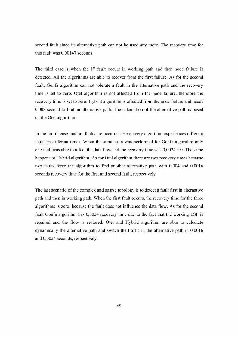
69
second fault since its alternative path can not be used any more. The recovery time for
this fault was 0,00147 seconds.
The third case is when the 1st fault occurs in working path and then node failure is
detected. All the algorithms are able to recover from the first failure. As for the second
fault, Gonfa algorithm can not tolerate a fault in the alternative path and the recovery
time is set to zero. Otel algorithm is not affected from the node failure, therefore the
recovery time is set to zero. Hybrid algorithm is affected from the node failure and needs
0,008 second to find an alternative path. The calculation of the alternative path is based
on the Otel algorithm.
In the fourth case random faults are occurred. Here every algorithm experiences different
faults in different times. When the simulation was performed for Gonfa algorithm only
one fault was able to affect the data flow and the recovery time was 0,0024 sec. The same
happens to Hybrid algorithm. As for Otel algorithm there are two recovery times because
two faults force the algorithm to find another alternative path with 0,004 and 0.0016
seconds recovery time for the first and second fault, respectively.
The last scenario of the complex and sparse topology is to detect a fault first in alternative
path and then in working path. When the first fault occurs, the recovery time for the three
algorithms is zero, because the fault does not influence the data flow. As for the second
fault Gonfa algorithm has 0,0024 recovery time due to the fact that the working LSP is
repaired and the flow is restored. Otel and Hybrid algorithm are able to calculate
dynamically the alternative path and switch the traffic in the alternative path in 0,0016
and 0,0024 seconds, respectively.
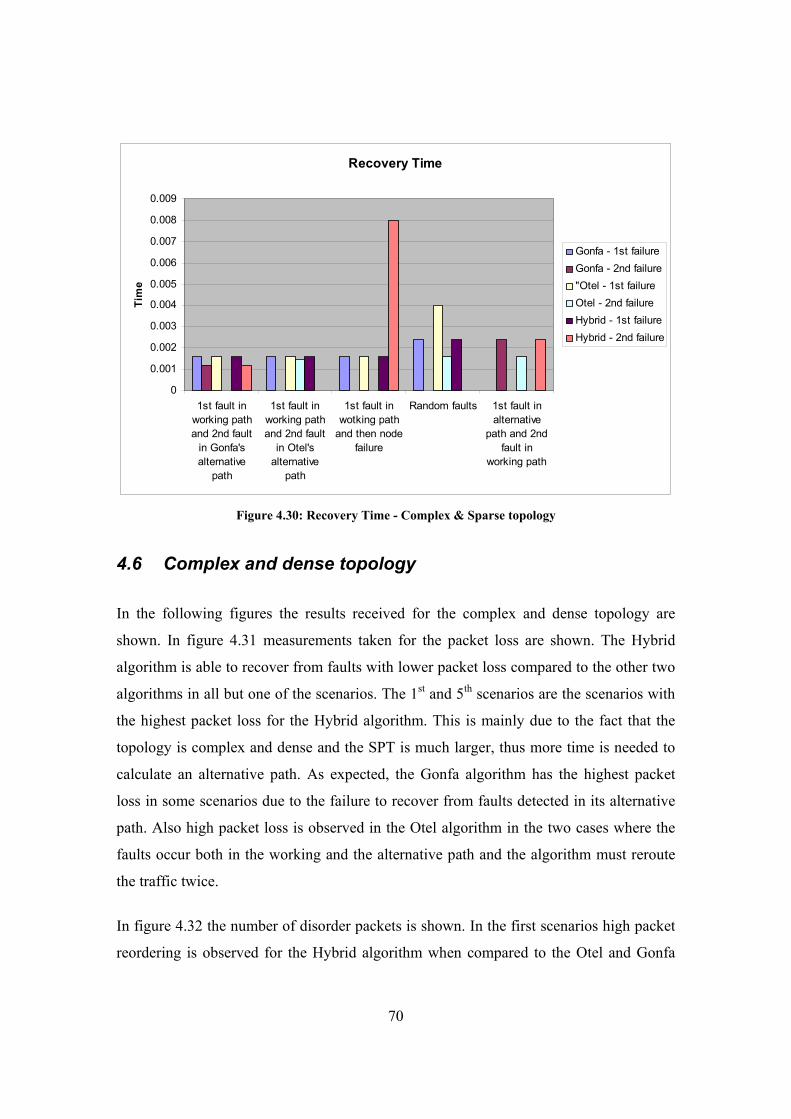
70
Recovery Time
0
0.001
0.002
0.003
0.004
0.005
0.006
0.007
0.008
0.009
1st fault inworking pathand 2nd fault
in Gonfa'salternative
path
1st fault inworking pathand 2nd fault
in Otel'salternative
path
1st fault inwotking path
and then nodefailure
Random faults 1st fault inalternative
path and 2ndfault in
working path
Tim
e
Gonfa - 1st failureGonfa - 2nd failure"Otel - 1st failureOtel - 2nd failureHybrid - 1st failureHybrid - 2nd failure
Figure 4.30: Recovery Time - Complex & Sparse topology
4.6 Complex and dense topology
In the following figures the results received for the complex and dense topology are
shown. In figure 4.31 measurements taken for the packet loss are shown. The Hybrid
algorithm is able to recover from faults with lower packet loss compared to the other two
algorithms in all but one of the scenarios. The 1st and 5th scenarios are the scenarios with
the highest packet loss for the Hybrid algorithm. This is mainly due to the fact that the
topology is complex and dense and the SPT is much larger, thus more time is needed to
calculate an alternative path. As expected, the Gonfa algorithm has the highest packet
loss in some scenarios due to the failure to recover from faults detected in its alternative
path. Also high packet loss is observed in the Otel algorithm in the two cases where the
faults occur both in the working and the alternative path and the algorithm must reroute
the traffic twice.
In figure 4.32 the number of disorder packets is shown. In the first scenarios high packet
reordering is observed for the Hybrid algorithm when compared to the Otel and Gonfa

71
algorithms. However, generally speaking, packet reordering is approximately the same
for the three algorithms except from the fourth case where the Otel algorithm experiences
the highest packet re-ordering.
Packet Loss
0
50
100
150
200
250
300
350
400
1st fault in workingpath and 2nd fault
in Gonfa'salternative path
1st fault in workingpath and 2nd faultin Otel's alternative
path
1st fault in workingpath and 2nd faultin common link forthe two alternative
path
1st fault in workingpath and 2nd fault
in commonalternative path forthe two algorithms
1st fault inalternative pathand 2nd fault in
working path
Num
ber o
f pac
kets
GonfaOtelHybrid
Figure 4.31: Packet Loss - Complex & Dense topology

72
Packet Reordering
0
5
10
15
20
25
30
35
40
45
50
1st fault in workingpath and 2nd fault
in Gonfa'salternative path
1st fault in workingpath and 2nd fault
in Otel'salternative path
1st fault in workingpath and 2nd faultin common link forthe two alternative
path
1st fault in workingpath and 2nd fault
in commonalternative path forthe two algorithms
1st fault inalternative pathand 2nd fault in
working path
GonfaOtelHybrid
Figure 4.32: Packet Reordering - Complex & Dense topology
Received Packets
0
100
200
300
400
500
600
700
800
900
1st fault inworking path and
2nd fault inGonfa's alternative
path
1st fault inworking path and2nd fault in Otel'salternative path
1st fault inworking path and
2nd fault incommon link for
the two alternativepath
1st fault inworking path and
2nd fault incommon
alternative path forthe two algorithms
1st fault inalternative pathand 2nd fault in
working path
Num
ber o
f Pac
kets
GonfaOtelHybrid
Figure 4.33: Received Packets - Complex & Dense topology
In figure 4.34 the amount of data transferred per second through links is shown. Here all
the algorithms in first three cases have the same throughput which is 0.45 Mb/sec.
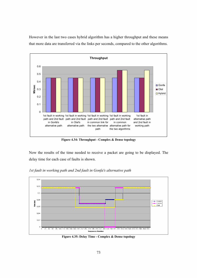
73
However in the last two cases hybrid algorithm has a higher throughput and these means
that more data are transferred via the links per seconds, compared to the other algorithms.
Throughput
0
0.1
0.2
0.3
0.4
0.5
0.6
1st fault in workingpath and 2nd fault
in Gonfa'salternative path
1st fault in workingpath and 2nd fault
in Otel'salternative path
1st fault in workingpath and 2nd faultin common link forthe two alternative
path
1st fault in workingpath and 2nd fault
in commonalternative path forthe two algorithms
1st fault inalternative pathand 2nd fault in
working path
Mb/
sec Gonfa
OtelHybrid
Figure 4.34: Throughput - Complex & Dense topology
Now the results of the time needed to receive a packet are going to be displayed. The
delay time for each case of faults is shown.
1st fault in working path and 2nd fault in Gonfa's alternative path
Figure 4.35: Delay Time - Complex & Dense topology
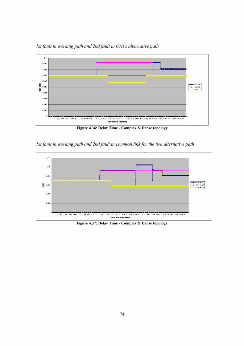
74
1st fault in working path and 2nd fault in Otel's alternative path
Figure 4.36: Delay Time - Complex & Dense topology
1st fault in working path and 2nd fault in common link for the two alternative path
Figure 4.37: Delay Time - Complex & Dense topology

75
1st fault in working path and 2nd fault in common alternative path for the two algorithms
Figure 4.38: Delay Time - Complex & Dense topology
1st fault in alternative path and 2nd fault in working path
Figure 4.39: Delay Time - Complex & Dense topology
The recovery time for each fault is shown in Figure 8. For the first scenario the fault is
detected in the working path and then in Gonfa’s alternative path. As expected the three
algorithms are able to recover from the first failure. The Hybrid algorithm has the least
recovery time in the first fault compared to the other algorithms. In the second failure the
Otel algorithm is not influenced and its recovery time is set to zero. The Hybrid algorithm
is able to find an alternative path in 0,0011 seconds. The Gonfa algorithm has 0,0019

76
recovery time due to the fact that one of the working LSP is repaired and the flow is
restored.
In the next scenario where the fault is detected in the working path and then in Otel’s
alternative path, it is observed that the three algorithms are able to restore the flow for the
first fault with the same recovery time. The second failure only influences the Otel
algorithm because the fault is detected to its alternative path and is able to recover from
failure in 0,0024 seconds. The Gonfa and Hybrid algorithms are not affected by the fault
and the recovery time is set to zero.
In the third scenario, where the fault is detected in the working path and then in a
common link of Otel’s and Gonfa’s alternative paths, it is observed that all algorithms are
able to recover from the first failure with the same recovery time. As for the second fault,
Gonfa has 0,0004 seconds recovery time due to the fact that the working path is repaired
and the flow is restored. The recovery time of Otel is set to zero, since during the
procedure of calculating an alternative path, the working LSP is repaired and the flow is
rerouted to the working path instantaneously. The Hybrid algorithm repairs the fault in
0,004 seconds. The results of the last scenario are justified as in this scenario.
The next scenario of the complex and sparse topology is to detect a fault first in the
alternative path and then in the working path. When the first fault occurs, the recovery
time for the three algorithms is zero, because the fault does not influence their data flow.
As for the second fault, Gonfa has 0,0012 recovery time due to the fact that the working
LSP is repaired and the flow is restored. Both Otel and Hybrid are able to calculate
dynamically an alternative path and switch the traffic in the alternative path in 0,0012
seconds.

77
Recovery Time
0
0.0005
0.001
0.0015
0.002
0.0025
0.003
0.0035
0.004
0.0045
1st fault inworking path
and 2nd fault inGonfa's
alternative path
1st fault inworking path
and 2nd fault inOtel's alternative
path
1st fault inworking path
and 2nd fault incommon link for
the twoalternative path
1st fault inalternative pathand 2nd fault in
working path
1st fault inworking path
and 2nd fault incommon
alternative pathfor the twoalgorithms
Tim
e
Gonfa - 1st failureGonfa - 2nd failureOtel - 1st failureOtel - 2nd failureHybrid - 1st failureHybrid - 2nd failure
Figure 4.40: Recovery Time- Complex & Dense topology
4.7 Analysis of Results Based on the obtained simulation results, we draw the following conclusions regarding
the proposed Hybrid algorithm. First of all, each topology category gives (as expected)
different results for the same failure scenario. The network topology plays a significant
role in the Hybrid algorithm (and Otel) due to the fact that the alterative path is calculated
via the SPT, which basically represents the topology. Based on the obtained results a
small increase on packet loss, packet reordering and the recovery time is observed while
the network topology is becoming more complex and dense. This is due to the fact that
when SPT becomes bigger, it requires more time to be updated (for the computation of a
new alternative path). Moreover it appears that the performance of the algorithm depends
on two correlated factors: (i) the size of the SPT subtree, affected by the failure and (ii)
the number of links originating from nodes outside the subtree but incident to subtree
nodes.
Furthermore, two different SPTs can give different results in the same scenarios. This is
derived from the different recovery times given by the Otel and Hybrid algorithms in the
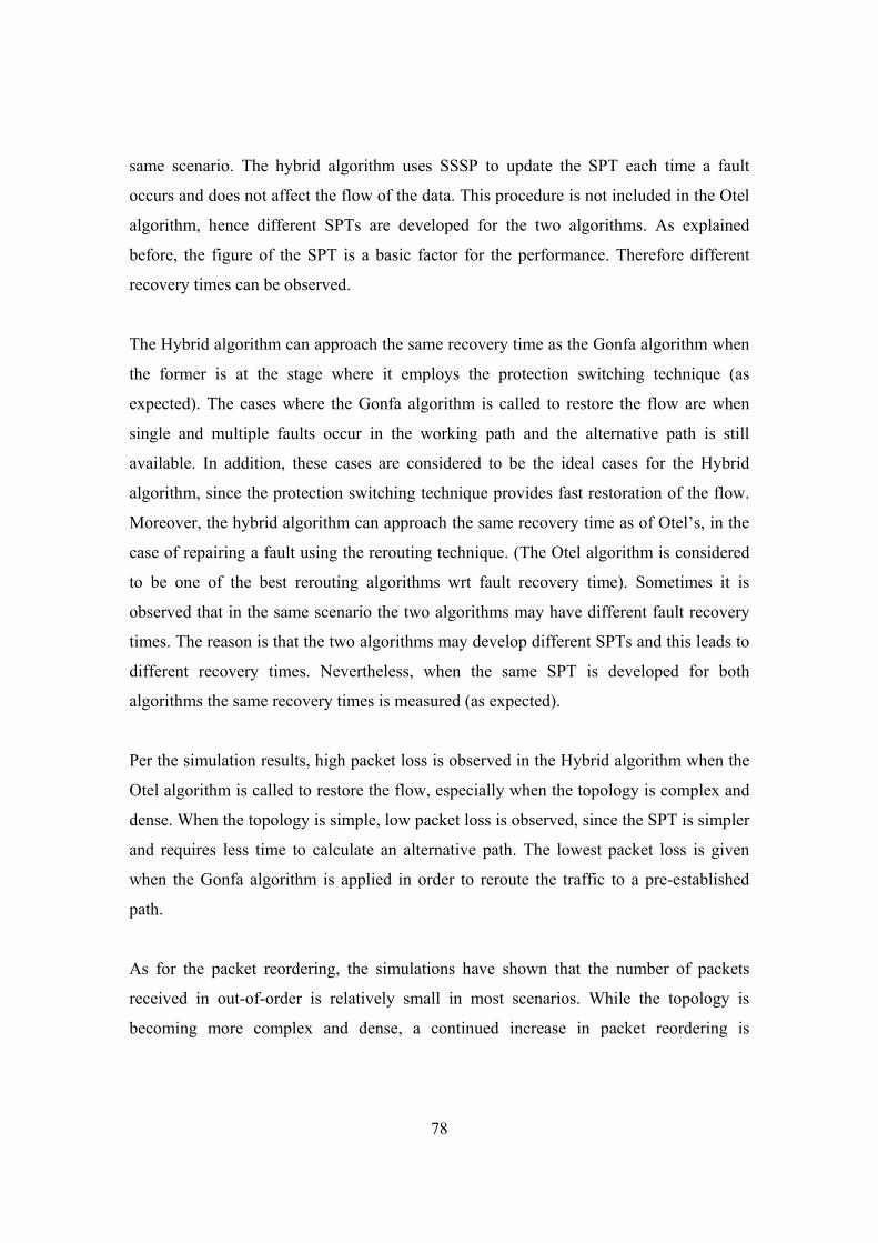
78
same scenario. The hybrid algorithm uses SSSP to update the SPT each time a fault
occurs and does not affect the flow of the data. This procedure is not included in the Otel
algorithm, hence different SPTs are developed for the two algorithms. As explained
before, the figure of the SPT is a basic factor for the performance. Therefore different
recovery times can be observed.
The Hybrid algorithm can approach the same recovery time as the Gonfa algorithm when
the former is at the stage where it employs the protection switching technique (as
expected). The cases where the Gonfa algorithm is called to restore the flow are when
single and multiple faults occur in the working path and the alternative path is still
available. In addition, these cases are considered to be the ideal cases for the Hybrid
algorithm, since the protection switching technique provides fast restoration of the flow.
Moreover, the hybrid algorithm can approach the same recovery time as of Otel’s, in the
case of repairing a fault using the rerouting technique. (The Otel algorithm is considered
to be one of the best rerouting algorithms wrt fault recovery time). Sometimes it is
observed that in the same scenario the two algorithms may have different fault recovery
times. The reason is that the two algorithms may develop different SPTs and this leads to
different recovery times. Nevertheless, when the same SPT is developed for both
algorithms the same recovery times is measured (as expected).
Per the simulation results, high packet loss is observed in the Hybrid algorithm when the
Otel algorithm is called to restore the flow, especially when the topology is complex and
dense. When the topology is simple, low packet loss is observed, since the SPT is simpler
and requires less time to calculate an alternative path. The lowest packet loss is given
when the Gonfa algorithm is applied in order to reroute the traffic to a pre-established
path.
As for the packet reordering, the simulations have shown that the number of packets
received in out-of-order is relatively small in most scenarios. While the topology is
becoming more complex and dense, a continued increase in packet reordering is
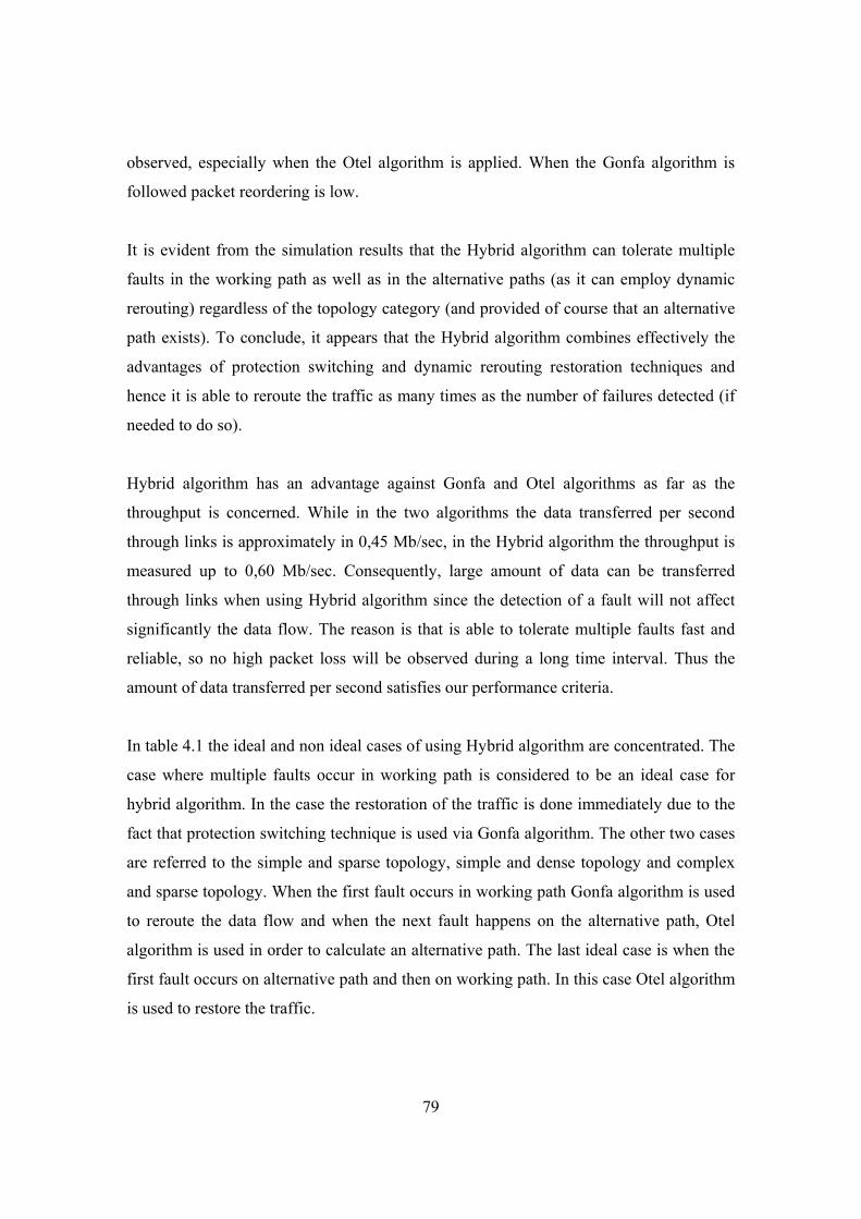
79
observed, especially when the Otel algorithm is applied. When the Gonfa algorithm is
followed packet reordering is low.
It is evident from the simulation results that the Hybrid algorithm can tolerate multiple
faults in the working path as well as in the alternative paths (as it can employ dynamic
rerouting) regardless of the topology category (and provided of course that an alternative
path exists). To conclude, it appears that the Hybrid algorithm combines effectively the
advantages of protection switching and dynamic rerouting restoration techniques and
hence it is able to reroute the traffic as many times as the number of failures detected (if
needed to do so).
Hybrid algorithm has an advantage against Gonfa and Otel algorithms as far as the
throughput is concerned. While in the two algorithms the data transferred per second
through links is approximately in 0,45 Mb/sec, in the Hybrid algorithm the throughput is
measured up to 0,60 Mb/sec. Consequently, large amount of data can be transferred
through links when using Hybrid algorithm since the detection of a fault will not affect
significantly the data flow. The reason is that is able to tolerate multiple faults fast and
reliable, so no high packet loss will be observed during a long time interval. Thus the
amount of data transferred per second satisfies our performance criteria.
In table 4.1 the ideal and non ideal cases of using Hybrid algorithm are concentrated. The
case where multiple faults occur in working path is considered to be an ideal case for
hybrid algorithm. In the case the restoration of the traffic is done immediately due to the
fact that protection switching technique is used via Gonfa algorithm. The other two cases
are referred to the simple and sparse topology, simple and dense topology and complex
and sparse topology. When the first fault occurs in working path Gonfa algorithm is used
to reroute the data flow and when the next fault happens on the alternative path, Otel
algorithm is used in order to calculate an alternative path. The last ideal case is when the
first fault occurs on alternative path and then on working path. In this case Otel algorithm
is used to restore the traffic.

80
The two cases that are not considered to be ideal for hybrid algorithm have as
requirement complex and dense topology. The first case is when the first fault occurs in
working path and then in alternative path and the other case is when the first fault occurs
on alternative path and then on working path. Both cases use Otel algorithm to calculate
alternative path when Gonfa can not be applied. But the calculation of the alternative path
will be done using SPT, which in a complex and dense topology becomes bigger and
makes more complicated the procedure of finding the alternative path.
Some times Hybrid algorithm has the same results as Gonfa and some times as Otel.
These cases are shown in table 4.2. Hybrid algorithm has the same results as Gonfa when
a single or multiple faults occur in the working path. Due to the fact that the alternative
path is available the traffic can be restored using Gonfa algorithm. Also the same
backwards and alternative LSPs are established for the both algorithms. As a result, the
packet loss, packet reordering, received packets throughput and recovery time will be the
same for both algorithms. On the other hand hybrid algorithm has the same results as the
Otel the same SPT is developed, otherwise different recovery times will be measured.
When this case occurs then the same packet loss, packet reordering, received packets
throughput and recovery time will be given by both algorithms.
Ideal Cases Non ideal cases 1
Multiple faults in working path
Complex and dense topology - 1st fault in working LSP then in alternative LSP
2
1st fault in working LSP then in alternative LSP
Complex and dense topology - 1st fault in alternative LSP then in working LSP
3
1st fault in alternative LSP then in working LSP
Table 4.1: Ideal and non ideal cases for Hybrid algorithm
Hybrid has the same results as Gonfa Hybrid has the same results as Otel
1 Single fault in working path The two algorithms have the SPT
2 Multiple faults in working path
Table 4.2: Cases where Hybrid have the same results as Gonfa and as Otel

81
5 Conclusion Multi-protocol Label Switching (MPLS) has become an attractive technology of choice
for Internet backbone service providers. MPLS features the ability to perform traffic
engineering and provides support for Quality of Service traffic provisioning. This has
resulted in increasing interest in MPLS network reliability and survivability. Therefore
each algorithm proposed for the restoration of MPLS networks must be reliable and fast.
The recovery of the MPLS network is based on the algorithm that is applied in order to
detect the faults and route the data flow in an alternative path. There are various
algorithms that have been proposed in the bibliography. Each algorithm proposed for
fault tolerance in MPLS, applies different techniques in order to be able to tolerate faults
in the MPLS network and to satisfy specific criteria selected by the algorithm. Also, one
can observe that all current algorithms are either employing protection switching or
rerouting technique.
The algorithm presented in this paper is the first hybrid algorithm that employs both
protection switching and path rerouting restoration mechanisms in an effort to perform
well in a number of important criteria. The Hybrid algorithm combines effectively both
mechanisms and decreases the fault recovery time, reduces the packet loss and packet
reordering in several cases (when compared with algorithms that employ only one of the
two mechanisms) and supports multiple link and node failures both on the working and
recovery paths.

82
6 Future Work This chapter points out a few aspects for future developments.
Various scenarios were developed in order to evaluate the Hybrid algorithm. However
some more scenarios can be performed but this time with more users, therefore more data
flows will be added to the scenarios. Consequently, the scenario will become more
realistic, closer to the current state of the network, where the demand grows for the
Internet to carry more traffic.
Furthermore, there has been an increasing need for current networks to carry Quality of
Service (QoS) or high priority traffic. An example of high priority traffic is Voice over IP
or video streaming and generally real time applications, which can not tolerate severe
delays because this may force the user to terminate the connection. As a result the hybrid
algorithm can be improved by adding some aspects which are considering restoration of
QoS traffic which MPLS supports.
Finally, Hybrid algorithm has the best results based on the simulation, on the four
selected criteria as far as the restoration of the MPLS network is concerned.
Consequently, Hybrid algorithm can not only be developed in NS-2 simulator but in a
real environment as well. A more realistic experimental evaluation in real environment
will lead to more realistic results and conclusions for the Hybrid algorithm.

83
References 1. Afek, Y., Bremler-Barr, A., Kaplan, H., Cohen, E., Merritt, M.: Restoration by Path
Concatenation: Fast Recovery of MPLS Paths. In Proceedings of the twentieth annual ACM symposium on Principles of distributed computing, pp. 43--52. (2001)
2. Ahn, G., Jang, J., Chun, W.: An Efficient Rerouting Scheme for MPLS-Based Recovery and Its Performance Evaluation. Telecommunication Systems, 19(3-4), pp. 481--495. (2002)
3. Altaman E., Jimenez, T.: NS simulator for beginners. Lecture notes, Los Andes University, France, (2003)
4. Andersson, L., Doolan, P., Feldman, N., Fredette, A., Thoma, B.: LDP Specification, RFC 3036, (2001).
5. Bartos, R., Raman, M.: A Heuristic Approach to Service Restoration in MPLS Networks. In Proceeding of ICC 2001, pp. 117--121. (2001)
6. Bartos, R., Raman, M.: A Scheme for Fast Restoration in MPLS Networks. In Proceedings of the Twelfth IASTED International Conference on Parallel and Distributed Computing Systems (PDSC), pp. 488--493. November (2000).
7. Bartos, R., Raman, M., Gandhi, A.: New Approaches to Service Restoration in MPLS-Based networks. In Proceedings of EUROCON 2001 International Conference on Trends in Communications, pp. 58--61. (2001)
8. Capone, A., Fratta, L., Martignon, F.: Dynamic Routing of Bandwidth Guaranteed Connections in MPLS Networks. Wireless and Optical Communications, 1(1), pp. 75--86. (2003)
9. Chen, J., Chiou, C.C, Wu, S.L.: A Fast Path Recovery Mechanism for MPLS Networks. In Proceeding of ICOIN 2005, pp 58--65. (2005)
10. Chen T.M., Oh, T.H.: Reliable Services in MPLS. IEEE Communications Magazine, vol. 37, pp. 58--62. December (1999)
11. Fall, K., Varadhan, K.: The network simulator -ns-2. The VINT project. UC Berkeley, LBL, USC/ISI, and Xerox PARC, http://www.isi.edu/nsnam/ns/.
12. Gaeil, A., Woojik, C.: Overview of MPLS Network Simulator: Design and Implementation. Technical report, Department of Computer Engineering, Chungnam National University, Korea, (1999)
13. Gonfa, L.H.: Enhanced Fast Rerouting Mechanisms for Protected Traffic in MPLS Networks. Phd Thesis, Technical University of Catalonia, February (2003)
14. Haskin, D., Krishnan, R.: A Method for Setting an Alternative Label Switched Paths to Handle Fast Reroute. Internet draft (2000)
15. Hong, D.W., Hong, C.S.: A Rerouting Scheme with Dynamic Control of Restoration Scope for Survivable MPLS Network. In Proceeding of ICOIN 2005, pp. 233--243. (2005)
16. k Disjoint Shortest Paths – k DSP, http://www.mat.uc.pt/~eqvm/OPP/KSPP/KSPP.html, Access Date: 25/11/2007
17. Kodialam, M., Lakshman, T. V.: Minimum Interference Routing with Applications to MPLS Traffic Engineering. In Proceedings of IEEE Infocom, pp. 884--893. (2000)
18. Kurose, J.F., Ross, K.W.: Computer Networking – A Top-Down Approach Featuring the Internet, 3rd Edition, Addison-Wesley, 2004.

84
19. Lin, J.W., Liu, H.Y.: An Efficient Fault-Tolerant Approach for MPLS Network Systems. In proceedings of ISPA 2004, pp. 815--824.(2004)
20. Makam, S., Sharma, V., Owens, K., Huang, C.: Protection/Restoration Mechanism for MPLS Networks. Work in progress, Internet draft <draft-makam-mplsprotection-00.txt>, (1999)
21. Menth, M., Milbrandt, J., Reifert, A.: Self-Protecting Multipaths - A Simple and Resource-Efficient Protection Switching Mechanism for MPLS Networks. In Proceeding of IFIP-TC6 Networking Conference (Networking), (Athens, Greece), pp. 526--537. May (2004)
22. Otel, F.D.: On Fast Computing Bypass Tunnel Routes in MPLS-Based Local Restoration. In proceeding of High Speed Networks and Multimedia Communications 5th IEEE International Conference, pp. 234--238. February (2002)
23. Petersson, J.M.: MPLS Based Recovery Mechanisms. Master Thesis, University of Oslo, (2005).
24. Pu, J., Manning, E., Shoja, G.C.: Reliable Routing in MPLS Networks. In Proceedings of Communications and Computer Networks, (2002)
25. Rosen, E., Viswanathan, A., Callon, R.: Multiprotocol Label Switching Architecture. RFC 3031, January (2001)
26. Sharma, V., Hellstrand, F: Framework for Multi-Protocol Label Switching (MPLS)-based Recovery, RFC 3469, (2003)
27. Yoon, S., Lee, H., Choi, D., Kim, Y., Lee, G., Lee, M.: An Efficient Recovery Mechanism for MPLS-based Protection LSP. In Proceedings of Joint 4th IEEE International Conference on ATM (ICATM 2001) and High Speed Intelligent Internet Symposium, pp. 75--79. April (2001)