a hybrid coordinate ocean model for shelf sea simulation · a hybrid coordinate ocean model for...
TRANSCRIPT

A Hybrid Coordinate Ocean Model for shelf
sea simulation
Nina Gjerde Winther a,∗, Geir Evensen b,a
aMohn-Sverdrup Center/Nansen Environmental and Remote Sensing Center,Bergen, Norway
bHydro Research Center, Bergen, Norway
Abstract
The general circulation in the North Sea and Skagerrak is simulated using theHybrid Coordinate Ocean Model (HYCOM). Although HYCOM was originally de-veloped for simulations of the open ocean, it has a design which should make itapplicable also for coastal and shallow shelf seas. Thus, the objective of this studyhas been to examine the skills of the present version of HYCOM in a coastal shelfapplication, and to identify the areas where HYCOM needs to be further developed.To demonstrate the capability of the vertical coordinate in HYCOM, three exper-iments with different configurations of the vertical coordinate were carried out. Ingeneral, the results from these experiments compares quite well with in situ andsatellite data, and the water masses and the general circulation in the North Seaand Skagerrak is reproduced in the simulations. Differences between the three ex-periments are small compared to other errors, which are related to a combined effectof model setup and properties of the vertical mixing scheme. Hence, it is difficult toquantify which vertical coordinate configuration works best for the coastal region.It is concluded that HYCOM can be used for simulations of coastal and shelf seas,and further suggestions for improving the model results are given. Since HYCOMalso works well in open ocean and basin scale simulations, it may allow for a realisticmodelling of the transition region between the open ocean and coastal shelf seas.
Key words: HYCOM · hybrid coordinate · shelf sea · North Sea · Skagerrak
∗ Corresponding authorEmail addresses: [email protected] (Nina Gjerde Winther),
[email protected] (Geir Evensen).
Preprint submitted to Ocean Modelling 24 January 2006
1 Introduction
One of the key issues in numerical ocean modelling is the choice of verticalcoordinate system and one of three formulations are normally used. Theseare the z-level coordinate which uses the depth as vertical coordinate, theterrain following sigma coordinate which scales with depth, and the isopycnalcoordinate which uses a discretization in potential density referenced to agiven pressure.
The z-level models have traditionally been used for basin scale simulations. Asdiscussed by Haidvogel and Beckmann (1998) z-level models must representirregular topography as a number of steps, and have therefore difficulties ofrepresenting strongly varying topography with a limited number of levels.Hence, z-level models are not widely used for coastal applications.
Sigma coordinate models have become a standard for modelling coastal andshallow or unstratified seas. The main advantages of these models are a smoothrepresentation of bottom topography and their ability to retain high verticalresolution near the surface and the sea floor, allowing for a realistic modellingof the surface and bottom boundary layers. The main drawback has been theoccurrence of the so-called pressure gradient error (see e.g. Mellor et al., 1998),although the introduction of advanced numerical schemes have significantlyreduced the impact of these errors (Shchepetkin and McWilliams, 2003). Fur-ther, in stratified regions sigma coordinate models will typically introduceunphysical numerical mixing across isopycnals.
There are many advantages of using isopycnal coordinates, including the properconservation of deep water masses during very long time integrations whereone has total control of the diapycnal mixing. This has motivated the devel-opment of isopycnal ocean models, in particular for basin scale and climatesimulations. However, these models cannot be used in shelf seas unless thereis a significant stratification and they have been limited by the use of a single-layer bulk representation of the mixed layer.
The Hybrid Coordinate Ocean Model (HYCOM) by Bleck (2002) is an out-growth of the Miami Isopycnal Coordinate Ocean Model (MICOM; Bleck andSmith, 1990). The major improvements in HYCOM relative to MICOM isthe introduction of a hybrid vertical coordinate, which allows for the use ofcoordinate formulations suitable for different ocean regimes. The hybrid coor-dinate is typically isopycnal in the open, stratified ocean, but there is a smoothtransition to z-level coordinates in the mixed layer and a transition to sigmacoordinates in shallow coastal regions. This approach allows for high verticalresolution close to the surface and in shallow regions, and has also allowed forimplementation of non-slab vertical mixing schemes like the K-Profile Param-
2

eterization (KPP; Large et al., 1994).
HYCOM was originally developed as an open ocean model, and has beenevaluated in basin scale studies (Chassignet et al., 2003; Halliwell, 2004; Shajiet al., 2005). On the other hand, the objective of this study has been to testthe skills of the present version of HYCOM on a coastal application, and toidentify areas where HYCOM needs to be further developed. The introductionof the hybrid coordinate gives HYCOM the potential to be extended from theopen ocean to coastal and shelf seas, so the question addressed in this study isif HYCOM can be used to realistically model both the open ocean and coastalshelf regions, and in particular, will it provide a realistic simulation of thetransition region along the shelf break? These questions are now addressedin an application of HYCOM for the North Sea and Skagerrak which is thefirst systematic effort to validate HYCOM in a coastal application using anextensive observed data set.
The North Sea is a shelf sea that lies between Norway, the British Isles andthe European Continent. The current system in the North Sea is characterizedby a southward inflow of Atlantic water and the northward flowing Norwegiancoastal current (NCC). The North Sea is a shallow sea, with two thirds of theregion having depths shallower than 100m. The exception is the Norwegiantrench, which has depths exceeding 700m. This special topography controlsthe circulation to a great extent. The saline Atlantic water enters the NorthSea at its northern boundary and also through the English channel. It followsthe topography, and is mixed with fresher and colder water from rivers. Whenit reaches the inner part of Skagerrak, the area between Denmark, Swedenand Norway, it meets brackish water from the Baltic and turns northward. Asit reaches Norway, it follows the coast westwards and becomes the NorwegianCoastal Current. The NCC is known as a chaotic current, with high mesoscaleactivity, but in general it follows the coast northwards. This leads to an overallcyclonic circulation in the North Sea.
The North Sea is a challenging region for any coastal circulation model withit’s large range of depths and various water masses and we believe it providesa good test case for HYCOM in this study.
Some important HYCOM features are presented in Section 2. Section 3 de-scribes the model setup, and Section 4 presents the measurements used formodel evaluation. In Section 5 model results and measurements are comparedand discussed. Finally, Section 6 sums up the work done in this study andgives the conclusions.
3

2 HYCOM features
For details about the prognostic equations in HYCOM we refer to Bleck(2002), but the important parts that involve the hybrid vertical coordinateand that makes HYCOM different from other numerical codes typically usedfor shelf sea simulations are summarized in the following. The continuity equa-tion in HYCOM is given by
∂
∂ts
(
∂p
∂s
)
+ ∇s ·
(
v∂p
∂s
)
+∂
∂s
(
s∂p
∂s
)
= 0, (1)
where v is the horizontal velocity vector, p is the pressure and s is an unspec-ified vertical coordinate that is held constant during partial differentiation.s∂p/∂s represents the vertical mass flux across an s surface, and is the termthat controls the movement and spacing of layer interfaces in HYCOM. This“grid generator” exploits the fact that all layers have an assigned target den-sity. Whenever the layer thickness tends to zero because this light water doesnot exist in the water column, this layer is used as a z-level coordinate withinthe mixed layer. This z-level coordinate is located in depth according to apredefined rule, which uses a minimum z-level thickness, δmin
p , a maximumz-level thickness, δmax
p , and a stretching factor, fp. These parameters controlthe z-level spacing and results in a top layer of thickness δmin
p and a minimumallowed thickness, bounded by δmax
p , for each layer given by
δn(k) = min(
δmaxp , δmin
p fpk−1
)
. (2)
In addition, there will be a transition to sigma coordinates in shallow regions,by specifying the number of layers that are to become sigma layers, Nσ, andtheir minimum allowed thickness, δmin
s . This gives a new expression for theminimum allowed thickness in each layer:
δn′(k) = max
[
δmins , min
(
δn,D
Nσ
)]
, (3)
where D is the water depth. This means that in a given model layer, thetransition occurs where the water depth becomes sufficiently shallow to makeD/Nσ < δn.
Advection of layer thicknesses in the continuity equation will introduce a ver-tical movement of the layer interfaces, also among the level coordinates nearthe surface. Further, horizontal diffusion of temperature and salinity in anisopycnic layer may lead to a deviation from the reference density. Therefore,at every time step, the ”grid generator“ needs to restore the coordinate sur-faces. Among the isopycnal coordinates there is a restoration towards targetdensities. If the layer is too dense the upper interface is moved upwards, i.e.there is a flux of lighter water across the interface. If the layer is less dense than
4

the target density, the lower interface is moved downward. For the z-level andsigma coordinates there will be a restoration towards their predefined locationsat depth. These points comprise the main features of the “grid generator”.
The standard vertical mixing scheme in HYCOM is currently the K-ProfileParameterization (KPP; Large et al., 1994), and was chosen also for this study.HYCOM contains three more sub-models for vertical mixing; Mellor-Yamadalevel 2.5 (MY; Mellor and Yamada, 1982), Price-Weller-Pinkel dynamical in-stability (Price et al., 1986) and NASA-GISS level 2 (Canuto et al., 2002).
The KPP scheme provides mixing for the entire water column by matchingthe parameterization of the surface boundary layer mixing with ocean interiormixing. Viscosity and diffusivities in the surface boundary layer are given by
Kx = hsblwx(σ)G(σ), (4)
where hsbl is the surface boundary layer depth, wx is a turbulent velocity scale,G is a non-dimensional shape function and σ is a non-dimensional verticalcoordinate ranging from 0 at the surface to 1 at the base of the boundarylayer.
For the discussion in this study the diagnosis of hsbl will be an important issue.A bulk Richardson number relative to the surface is given by
Rib(d) =(Br − B(d)) d
|Vr − V (d)2| + V 2t (d)
, (5)
where B is the buoyancy, V is the horizontal velocity and d is the distancefrom the surface. hsbl is diagnosed as the smallest depth at which a critical bulkRichardson number (Ric = 0.3) is reached. Subscript r refers to near-surfacevalues. Vt is an estimate of the turbulent velocity contribution to velocityshear.
Below the surface boundary layer there are three processes that contribute tothe interior mixing. These are shear-mixing, internal wave-generated mixingand double-diffusive mixing.
The shear-mixing term is parameterized as a function of the gradient Richard-son number,
Rig =N2
(∂U∂z
)2 + (∂V∂z
)2, (6)
where N is the buoyancy frequency and U and V are horizontal velocity
5
components. Shear-mixing viscosity is estimated as
νsh =
ν0 Rig < 0,
ν0
[
1 − (Rig/Ri0)2
]3
0 < Rig < Ri0,
0 Rig > Ri0,
(7)
where ν0 = 5.0 × 10⁻³ m2s−1 and Ri0 = 0.7.
For internal wave-generated mixing we use the same values that Durski et al.(2004) recommended for highly stratified coastal waters, namely 1.0 × 10⁻⁵
m2s−1 for momentum and 1.0 × 10⁻⁶ m2s−1 for potential density. For furtherdetails about the KPP scheme we refer to Large et al. (1994).
Earlier studies have shown that KPP compares favourably to MY in deepocean studies (Large et al., 1994; Large and Gent, 1999), but for simula-tions of the coastal ocean MY has become the standard. Durski et al. (2004)tested the performance of these two vertical mixing parameterizations in ide-alized continental shelf settings, and stated that the original KPP scheme isinadequate for application on a shallow continental shelf and that a bottomboundary layer parameterization should be appended when used in the coastalocean. This was not done in this study for two reasons. First of all, withinthe HYCOM consortium work is already in progress to implement and test anenhanced version of the KPP scheme. Secondly, as the ocean modelling com-munity are moving towards global grids with higher and higher resolution,the models will resolve more of the coastal shelf areas. In this context it isimportant to quantify how the choice of vertical mixing scheme will influencethe results. Hence, we kept the KPP as our vertical mixing sub-model to seehow it performs in a realistic shelf sea simulation.
3 Model Setup and Experiments
The overall model system consists of a two-level nested system where a largescale model feeds an intermediate resolution model with boundary conditions.This intermediate model provides boundary conditions needed by the highresolution model covering the North Sea and Skagerrak (Figure 1).
Boundary conditions are treated differently depending on whether the vari-ables are barotropic or baroclinic. For the slowly varying variables, i.e. baro-clinic velocities, temperature, salinity and layer interfaces, the boundary con-ditions are based on the flow relaxation scheme (FRS; Davies, 1983). Thismeans that we use a one way nesting scheme where the boundary conditionsof the regional model are relaxed towards the output from the coarser large
6

0
5
10
15
20
25
30
60o
W 0 o
120
o E
180 oW
30 oS
30
o N
60o N
0
200
400
600
800
1000
1200
1400
1600
5oW 0o 5oE 10oE 15oE
51oN
54oN
57oN
60oN
63oN
Ytre Utsira
Lista
Fig. 1. Left: A two-level nested model system, where the large scale model covers theAtlantic and Arctic ocean. Surface temperature is shown in colours and Arctic seaice extent in white. Right: Topography of the nested high resolution regional model.The black lines and red dots show the locations where in situ data are present. Thegreen dots show the location of river input that are used in this model setup.
scale model. For the barotropic variables the relaxation approach requirescareful treatment to avoid reflection of waves at the open model boundaries.In HYCOM the barotropic model is a hyperbolic wave equation for pressureand vertically integrated velocities. Following an approach outlined by Brown-ing and Kreiss (1982, 1986), it is possible to compute the barotropic boundaryconditions exactly while taking into consideration both the waves propagatinginto the regional model from the external solution and the waves propagatingout through the boundary from the regional model.
All grids were created with the conformal mapping tools of Bentsen et al.(1999). The large scale model has a variable resolution with approximately15-20 km grid cells in the Gulf Stream region, and with gradually coarser gridmoving into the South Atlantic and the Arctic Ocean. This model ensuresthat the overall general circulation and water masses in the North Atlanticand its seasonal variability are properly represented. The intermediate modelcovers all of the North Sea and the Atlantic Margin including the deep watersbetween Spain, Iceland and Norway. This model has about 7 km resolution,which is sufficient to provide realistic and fairly detailed circulation patternalong the Atlantic Margin. A higher resolution model is needed to ensuregood representation of the mesoscale variability and its energetics. Thus, aresolution of 4 km is used for the regional model covering the North Sea andSkagerrak.
Note that 4 km is normally too coarse to properly represent the mesoscaledynamics of the NCC, see e.g. Johannessen et al. (1989); Ikeda et al. (1989);Haugan et al. (1991); Oey and Chen (1992) which indicated that a model of2 km resolution is needed. However, we have compensated for resolution by
7

implementing a fourth order numerical scheme for the advection terms in themomentum equation which improves the dynamical representation of potentialvorticity. In practical applications this leads to similar results with half theresolution compared to the original version of HYCOM as shown by Wintheret al. (2005).
The large scale model is coupled to an ice module, which consists of both adynamic and a thermodynamic ice model. The dynamic ice model uses theElastic-Viscous-Plastic (EVP) rheology of Hunke and Dukowicz (1999). Thethermodynamic ice model is described by Drange and Simonsen (1996).
The topography used was interpolated to the model grid using the GeneralBathymetry Map of the Oceans (GEBCO), which operates under the auspicesof the International Hydrographic Organisation and the United Nations’ (UN-ESCO) Intergovernmental Oceanographic Commission. The resolution is oneminute.
The synoptic forcing fields were temperature, wind and humidity (determinedfrom dew-point temperatures) fields from the European Center for Medium-Range Weather Forecasting (ECMWF). Clouds are based on climatologiesfrom the Comprehensive Ocean and Atmosphere Dataset (COADS; Slutzet al., 1985), while precipitation is based on the climatology of Legates andWillmott (1990). All atmospheric fields have a horizontal resolution of 0.5◦.River input is modelled as negative salinity flux, and the location of riversources included around the North sea and Skagerrak are shown as greendots in Figure 1. At the surface the ocean model uses a weak temperature andsalinity relaxation towards the General Digital Environmental Model (GDEM)oceanic climatology (Teague et al., 1990).
To ensure a proper representation of the Baltic inflow to the North Sea model,a barotropic volume flux is included at the eastern boundary (see Figure 1).Values used to specify the volume flux are monthly climatology data and theBaltic water has been given a salinity of 8 psu.
The regional model includes tides, which are specified as a barotropic forcingat the open boundaries. The data set used originates from the University ofTexas and is based on several years of altimeter data collected by the TOPEXsatellite. Eight constituents are specified at the boundaries; K1, O1, P1, Q1,M2, N2, S2 and K2. These constituents make up a significant portion of thetidal signal, and are considered sufficient in this study.
The vertical discretization uses 22 hybrid layers, with target densities refer-ences to σ0 (i.e., density at atmospheric pressure minus 1000 kgm−3) in therange from 21.80 to 28.11. These were chosen to represent water masses andresolve the mixed layer in the Atlantic and Arctic ocean and are thereforenot ideal for this coastal application. Note that the lightest layers in this dis-
8

130 135 140I-index
0
100
200
Dep
th
Exp. 1
130 135 140I-index
0
100
200
Dep
th
Exp. 2
130 135 140I-index
0
100
200
Dep
th
Exp. 3
Fig. 2. Illustration of the vertical layer interfaces for the three different experiments.Parameters used to set-up these experiments are given in Table 1.
cretization are primarily used to describe the surface mixed layer, as they areusually too light to describe interior water masses in the ocean. This set-up isvalid for the outer models while for the North Sea model the target densitiesfor the top five layers were set to 0.1 to 0.5. This was done to avoid a collapsein the vertical coordinate when including rivers, since river input will causethe water density to get lower than the first target density.
Three different experiments with simulation period starting in January 1997and ending in July 1998, were carried out. The experiments differ in the waythe z- and sigma coordinates are defined and the parameters used are listedin Table 1. The resulting vertical discretizations from the different parametersets are illustrated in Figure 2.
The three experiments are summarized as follows:
Exp. 1 uses the same vertical coordinate set-up as the outer models, so thiswas the natural choice for the first simulation. As is seen in Figure 2, z-levelcoordinates are used both within the mixed layer and on the shelf.
Exp. 2 allows for a transition to sigma coordinates in shallow water regions.The purpose is to examine if sigma coordinates can improve the resultscompared to using standard z-levels as was done in Exp. 1. In Figure 2 itis seen that there is a transition to sigma coordinates only in very shallow
9
Exp. δminp δmax
p fp δmins δmax
s fs Nσ
(m) (m) (m) (m)
1 3 12 1.125 - - - 0
2 3 12 1.125 1 12 1.125 10
3 3 20 1.2 - - - 0
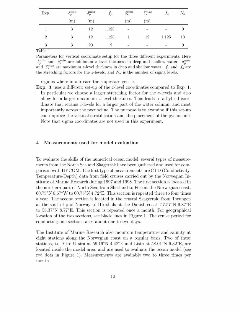
Table 1Parameters for vertical coordinate setup for the three different experiments. Hereδminp and δmin
s are minimum z-level thickness in deep and shallow water, δmaxp
and δmaxs are maximum z-level thickness in deep and shallow water, fp and fs are
the stretching factors for the z-levels, and Nσ is the number of sigma levels.
regions where in our case the slopes are gentle.Exp. 3 uses a different set-up of the z-level coordinates compared to Exp. 1.
In particular we choose a larger stretching factor for the z-levels and alsoallow for a larger maximum z-level thickness. This leads to a hybrid coor-dinate that retains z-levels for a larger part of the water column, and mostimportantly across the pycnocline. The purpose is to examine if this set-upcan improve the vertical stratification and the placement of the pycnocline.Note that sigma coordinates are not used in this experiment.
4 Measurements used for model evaluation
To evaluate the skills of the numerical ocean model, several types of measure-ments from the North Sea and Skagerrak have been gathered and used for com-parison with HYCOM. The first type of measurements are CTD (Conductivity-Temperature-Depth) data from field cruises carried out by the Norwegian In-stitute of Marine Research during 1997 and 1998. The first section is located inthe northern part of North Sea; from Shetland to Feie at the Norwegian coast,60.75◦N 0.67◦W to 60.75◦N 4.72◦E. This section is repeated three to four timesa year. The second section is located in the central Skagerrak; from Torungenat the south tip of Norway to Hirtshals at the Danish coast, 57.57◦N 9.87◦Eto 58.37◦N 8.77◦E. This section is repeated once a month. For geographicallocation of the two sections, see black lines in Figure 1. The cruise period forconducting one section takes about one to two days.
The Institute of Marine Research also monitors temperature and salinity ateight stations along the Norwegian coast on a regular basis. Two of thesestations, i.e. Ytre Utsira at 59.19◦N 4.48◦E and Lista at 58.01◦N 6.32◦E, arelocated inside the model area, and are used to evaluate the ocean model (seered dots in Figure 1). Measurements are available two to three times permonth.
10
The third type of data used for model evaluation is Sea Surface Temperature(SST) from the NOAA satellite (Vazquez et al., 1998). The product containsdata with different spatial and temporal resolutions, but the data used herehave a spatial resolution of 9 km and are daily averages.
5 Model results and evaluation
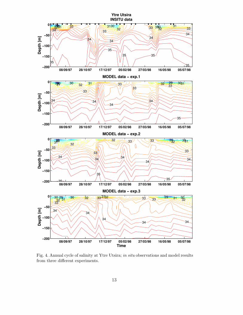
The model’s ability to simulate the correct water masses and circulation inthe North Sea and Skagerrak was first studied using the measurements fromYtre Utsira described in section 4. Figure 3 and 4 compares measurementsof temperature and salinity, respectively, with model results from the threeexperiments. The figures show temperature and salinity for the upper 200mfrom August 1997 to July 1998. (The first half year of 1997 is used as thespin-up period.) Note the black marks at the upper part of first panel. Thesemarks indicate the dates when measurements were collected, and note thatmodel results were extracted for the exact same dates.
The annual cycle of temperature is quite well simulated with HYCOM. Ver-tical mixing dominates during winter, which results in small temperature dif-ferences between surface and bottom. Heating during spring/summer resultsin a well defined surface layer of about 50m. Surface layer thickness duringsummer is well represented in the model, but in late summer 1997 the upper20m is about 3◦C too cold in all experiments compared to observations. Karaet al. (2005) showed that sea surface temperature is sensitive to both solarattenuation coefficient and misrepresentation of land-sea mask in atmosphericforcing fields. These factors will influence the model results of sea surface tem-perature also in this study. We use a constant solar attenuation coefficient, andas mentioned previously the ECMWF fields have a resolution of 0.5◦, whichis very low compared to the ocean model.
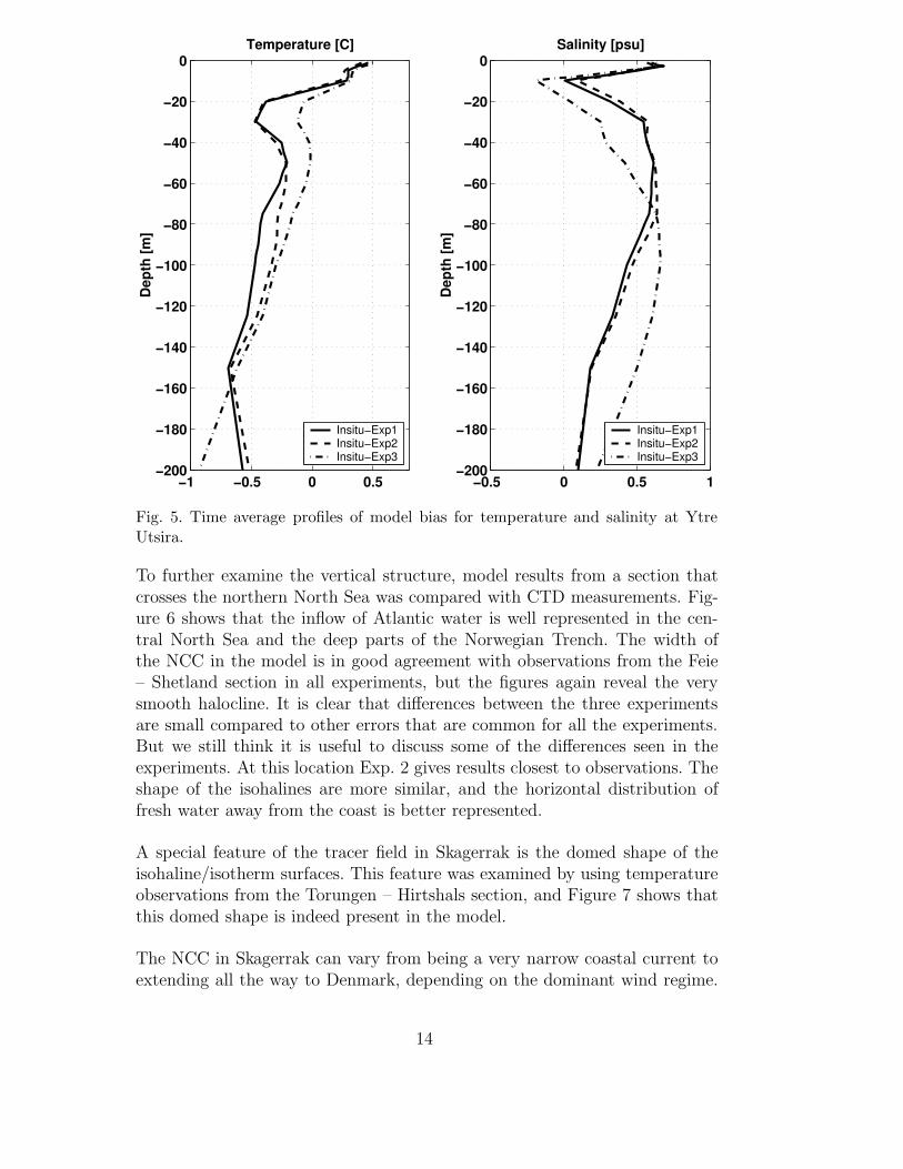
The main problem in the model is too smooth stratification between the NCCand the Atlantic water. This is specially evident in the salinity plots, andresults in too fresh water from about 50 to 150m, as seen in Figure 4. Theexperiments show some differences in temperature and salinity. This is fur-ther illustrated in Figure 5, which shows time average profiles of model bias oftemperature and salinity at the Ytre Utsira location. Exp. 2 strengthens thethermocline/halocline and lifts the Atlantic water towards shallower depthscompared to Exps. 1 and 3. On the other hand Exp. 3 strengthens the gra-dient in the upper 50m, and gives the most realistic results of the boundarylayer thickness. The exception is the fresh water input in December/January,which produces a fresh surface layer of about 50m depth, that none of theexperiments capture properly.
11

08/09/97 28/10/97 17/12/97 05/02/98 27/03/98 16/05/98 05/07/98−200
−150
−100
−50
0
Dept
h [m
]
Ytre UtsiraINSITU data
6
67
7
7
7
78
88
8
89
9
9910
1010
11
11
11
12
1213 131415161718
08/09/97 28/10/97 17/12/97 05/02/98 27/03/98 16/05/98 05/07/98−200
−150
−100
−50
0
Dept
h [m
]
MODEL data − exp.1
6
7
7
8
8
8
88
8
9
9
9
910
101011 11
1112
12131415
08/09/97 28/10/97 17/12/97 05/02/98 27/03/98 16/05/98 05/07/98−200
−150
−100
−50
0
Dept
h [m
]
MODEL data − exp.26
7
7
8
8
8
88
8
8
9
99
9 1010
10
1111
11 1212131415
08/09/97 28/10/97 17/12/97 05/02/98 27/03/98 16/05/98 05/07/98−200
−150
−100
−50
0
Time
Dept
h [m
]
MODEL data − exp.366
7
7
8
8
8
88
89
9
99
9 9
1010
1111
121213 1415
Fig. 3. Annual cycle of temperature at Ytre Utsira; in situ observations and modelresults from three different experiments.
12
08/09/97 28/10/97 17/12/97 05/02/98 27/03/98 16/05/98 05/07/98−200
−150
−100
−50
0
Dept
h [m
]
Ytre UtsiraINSITU data
2930 30 3031 31 31 3132 32 3233
3333 3334
34 3434
34
35
3535 35
35
08/09/97 28/10/97 17/12/97 05/02/98 27/03/98 16/05/98 05/07/98−200
−150
−100
−50
0
Dept
h [m
]
MODEL data − exp.12929 30303031 313132 32
33
33 3333
34 3434
34
35
08/09/97 28/10/97 17/12/97 05/02/98 27/03/98 16/05/98 05/07/98−200
−150
−100
−50
0
Dept
h [m
]
MODEL data − exp.22929 3030 3131 32 3232
3333
33
33
33
34 34 3434 34
3535
35
08/09/97 28/10/97 17/12/97 05/02/98 27/03/98 16/05/98 05/07/98−200
−150
−100
−50
0
Time
Dept
h [m
]
MODEL data − exp.32929 3030 30 3131
313232
323233
33 33 33
34 34
3434 34
Fig. 4. Annual cycle of salinity at Ytre Utsira; in situ observations and model resultsfrom three different experiments.
13
−1 −0.5 0 0.5−200
−180
−160
−140
−120
−100
−80
−60
−40
−20
0Temperature [C]
Dept
h [m
]
Insitu−Exp1Insitu−Exp2Insitu−Exp3
−0.5 0 0.5 1−200
−180
−160
−140
−120
−100
−80
−60
−40
−20
0Salinity [psu]
Dept
h [m
]Insitu−Exp1Insitu−Exp2Insitu−Exp3
Fig. 5. Time average profiles of model bias for temperature and salinity at YtreUtsira.
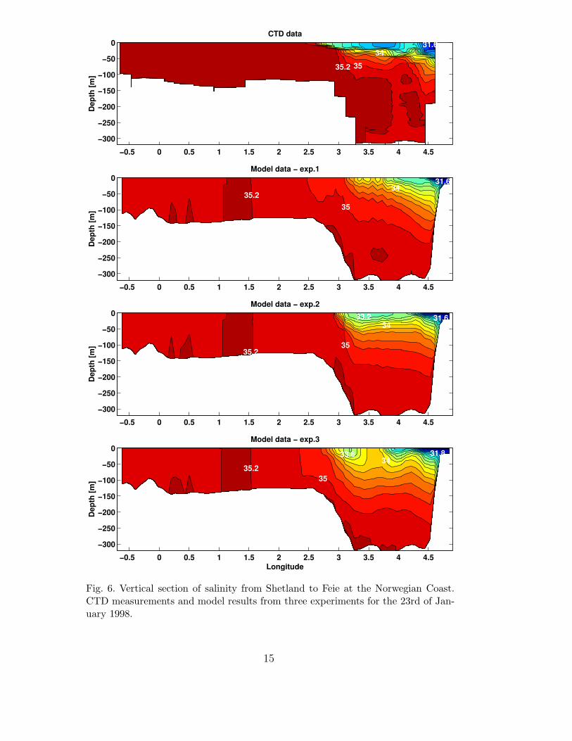
To further examine the vertical structure, model results from a section thatcrosses the northern North Sea was compared with CTD measurements. Fig-ure 6 shows that the inflow of Atlantic water is well represented in the cen-tral North Sea and the deep parts of the Norwegian Trench. The width ofthe NCC in the model is in good agreement with observations from the Feie– Shetland section in all experiments, but the figures again reveal the verysmooth halocline. It is clear that differences between the three experimentsare small compared to other errors that are common for all the experiments.But we still think it is useful to discuss some of the differences seen in theexperiments. At this location Exp. 2 gives results closest to observations. Theshape of the isohalines are more similar, and the horizontal distribution offresh water away from the coast is better represented.
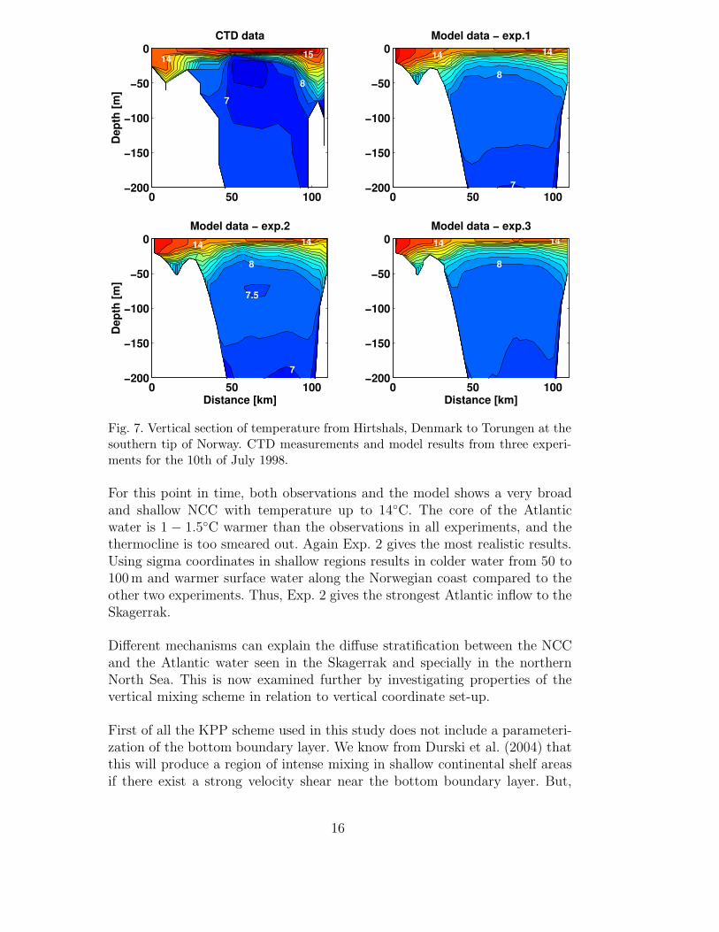
A special feature of the tracer field in Skagerrak is the domed shape of theisohaline/isotherm surfaces. This feature was examined by using temperatureobservations from the Torungen – Hirtshals section, and Figure 7 shows thatthis domed shape is indeed present in the model.
The NCC in Skagerrak can vary from being a very narrow coastal current toextending all the way to Denmark, depending on the dominant wind regime.
14
−0.5 0 0.5 1 1.5 2 2.5 3 3.5 4 4.5−300
−250
−200
−150
−100
−50
0CTD data
Dept
h [m
]
35.2 3534
31.6
−0.5 0 0.5 1 1.5 2 2.5 3 3.5 4 4.5−300
−250
−200
−150
−100
−50
0Model data − exp.1
Dept
h [m
]
35.235
3431.6
−0.5 0 0.5 1 1.5 2 2.5 3 3.5 4 4.5−300
−250
−200
−150
−100
−50
0Model data − exp.2
Dept
h [m
]
35.235
3433.2 31.6
−0.5 0 0.5 1 1.5 2 2.5 3 3.5 4 4.5−300
−250
−200
−150
−100
−50
0Model data − exp.3
Longitude
Dept
h [m
]
35.235
3433.6 31.8
Fig. 6. Vertical section of salinity from Shetland to Feie at the Norwegian Coast.CTD measurements and model results from three experiments for the 23rd of Jan-uary 1998.
15
0 50 100−200
−150
−100
−50
0CTD data
Dept
h [m
]7
8
1514
0 50 100−200
−150
−100
−50
0Model data − exp.1
8
7
1414
0 50 100−200
−150
−100
−50
0Model data − exp.2
Distance [km]
Dept
h [m
]
8
7
7.5
1414
0 50 100−200
−150
−100
−50
0Model data − exp.3
Distance [km]
8
14 14
Fig. 7. Vertical section of temperature from Hirtshals, Denmark to Torungen at thesouthern tip of Norway. CTD measurements and model results from three experi-ments for the 10th of July 1998.
For this point in time, both observations and the model shows a very broadand shallow NCC with temperature up to 14◦C. The core of the Atlanticwater is 1 − 1.5◦C warmer than the observations in all experiments, and thethermocline is too smeared out. Again Exp. 2 gives the most realistic results.Using sigma coordinates in shallow regions results in colder water from 50 to100m and warmer surface water along the Norwegian coast compared to theother two experiments. Thus, Exp. 2 gives the strongest Atlantic inflow to theSkagerrak.
Different mechanisms can explain the diffuse stratification between the NCCand the Atlantic water seen in the Skagerrak and specially in the northernNorth Sea. This is now examined further by investigating properties of thevertical mixing scheme in relation to vertical coordinate set-up.
First of all the KPP scheme used in this study does not include a parameteri-zation of the bottom boundary layer. We know from Durski et al. (2004) thatthis will produce a region of intense mixing in shallow continental shelf areasif there exist a strong velocity shear near the bottom boundary layer. But,
16
other processes within the KPP scheme also contribute to the very diffusestratification seen in the model results.
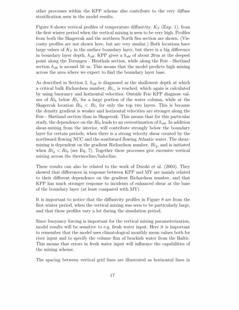
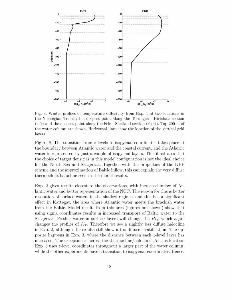
Figure 8 shows vertical profiles of temperature diffusivity, KT (Exp. 1), fromthe first winter period when the vertical mixing is seen to be very high. Profilesfrom both the Skagerrak and the northern North Sea section are shown. (Vis-cosity profiles are not shown here, but are very similar.) Both locations havelarge values of KT in the surface boundary layer, but there is a big differencein boundary layer depth, hsbl. KPP gives a hsbl of about 20m at the deepestpoint along the Torungen - Hirsthals section, while along the Feie - Shetlandsection hsbl is around 50 m. This means that the model predicts high mixingacross the area where we expect to find the boundary layer base.
As described in Section 2, hsbl is diagnosed as the shallowest depth at whicha critical bulk Richardson number, Ric, is reached, which again is calculatedby using buoyancy and horizontal velocities. Outside Feie KPP diagnose val-ues of Rib below Ric for a large portion of the water column, while at theSkagerrak location Rib < Ric for only the top two layers. This is becausethe density gradient is weaker and horizontal velocities are stronger along theFeie - Shetland section than in Skagerrak. This means that for this particularstudy, the dependence on the Rib leads to an overestimation of hsbl. In additionshear-mixing from the interior, will contribute strongly below the boundarylayer for certain periods, when there is a strong velocity shear created by thenorthward flowing NCC and the southward flowing Atlantic water. The shear-mixing is dependent on the gradient Richardson number, Rig, and is initiatedwhen Rig < Ri0 (see Eq. 7). Together these processes give excessive verticalmixing across the thermocline/halocline.
These results can also be related to the work of Durski et al. (2004). Theyshowed that differences in response between KPP and MY are mainly relatedto their different dependence on the gradient Richardson number, and thatKPP has much stronger response to incidents of enhanced shear at the baseof the boundary layer (at least compared with MY).
It is important to notice that the diffusivity profiles in Figure 8 are from thefirst winter period, when the vertical mixing was seen to be particularly large,and that these profiles vary a lot during the simulation period.
Since buoyancy forcing is important for the vertical mixing parameterization,model results will be sensitive to e.g. fresh water input. Here it is importantto remember that the model uses climatological monthly mean values both forriver input and to specify the volume flux of brackish water from the Baltic.This means that errors in fresh water input will influence the capabilities ofthe mixing scheme.
The spacing between vertical grid lines are illustrated as horizontal lines in
17
−6 −4 −2 0−200
−180
−160
−140
−120
−100
−80
−60
−40
−20
0
log10 KT [m2/s]
Dept
h [m
]
TOH
−6 −4 −2 0−200
−180
−160
−140
−120
−100
−80
−60
−40
−20
0
log10 KT [m2/s]
FSH
Fig. 8. Winter profiles of temperature diffusivity from Exp. 1 at two locations inthe Norwegian Trench; the deepest point along the Torungen - Hirtshals section(left) and the deepest point along the Feie - Shetland section (right). Top 200 m ofthe water column are shown. Horizontal lines show the location of the vertical gridlayers.
Figure 8. The transition from z-levels to isopycnal coordinates takes place atthe boundary between Atlantic water and the coastal current, and the Atlanticwater is represented by just a couple of isopycnal layers. This illustrates thatthe choice of target densities in this model configuration is not the ideal choicefor the North Sea and Skagerrak. Together with the properties of the KPPscheme and the approximation of Baltic inflow, this can explain the very diffusethermocline/halocline seen in the model results.
Exp. 2 gives results closest to the observations, with increased inflow of At-lantic water and better representation of the NCC. The reason for this is betterresolution of surface waters in the shallow regions, and this has a significanteffect in Kattegat; the area where Atlantic water meets the brackish waterfrom the Baltic. Model results from this area (figures not shown) show thatusing sigma coordinates results in increased transport of Baltic water to theSkagerrak. Fresher water in surface layers will change the Rib, which againchanges the profiles of KT . Therefore we see a slightly less diffuse haloclinein Exp. 2, although the results still show a too diffuse stratification. The op-posite happens in Exp. 3, where the distance between each z-level layer hasincreased. The exception is across the thermocline/halocline. At this locationExp. 3 uses z-level coordinates throughout a larger part of the water column,while the other experiments have a transition to isopycnal coordinates. Hence,
18

Fig. 9. Global wavelet power spectra of HYCOM SST, Exps. 1 and 2, and AVHRRSST from the 14th of May 1998.
Exp. 3 has a higher vertical resolution here, and a slight improvement is seen.
To evaluate the mesoscale structure in the NCC, wavelet analysis of SST wasperformed for both satellite data and model results (Figure 9). SST from 14thof May 1998 was chosen, since this was one of the few days of cloud free condi-tions that coincides with the simulation period. Data was extracted along 4◦Eand from 59.3◦N to 62◦N, which gives a section trough the mesoscale struc-ture in the NCC. Wavelet analysis was performed using the Matlab package byTorrence and Compo (1998). Both observations and model results show globalwavelet energy spectra with similar shape and energy focused on a wavelengthinterval around 50 to 120 km. Unfortunately data from Exp. 3 was lost for thisparticular date.
All examples above give an evaluation of the model either at a specific pointin space (Ytre Utsira) or at a specific point in time (vertical sections andwavelet analysis). Therefore, transports were computed from the model resultsto evaluate the mean flows in the model. Rodhe (1996) reviews the large-scale hydrography of Skagerrak, and states that the inflow from the west issomewhere between 0.5 and 1.0 Sv. Danielssen et al. (1997) estimated thetransport in the upper 100m to be about 1 (±0.5) Sv. In Exps. 1, 2 and 3 wepredicted transport values of 1.12, 1.16 and 1.04 Sv, respectively, for the inflowto the Skagerrak. Thus, all three values correspond well with observations.
19
6 Conclusions
In this study we have used HYCOM to simulate the circulation in the NorthSea and Skagerrak. In general, HYCOM gave good results in comparison withdifferent types of observations. It was seen that different water masses arewell represented in the simulations, and that the general circulation is wellreproduced. In addition we found that the dynamics of the chaotic NCC is wellsimulated in the model. Three experiments with different configurations of thevertical coordinate were carried out. Differences between the three experimentsare small compared to other errors, and weaknesses related to properties of thevertical mixing scheme in combination with the model setup are quantified.It is concluded that HYCOM can be used for simulations of coastal and shelfseas, but in different areas the model should be further developed.
To use HYCOM for the coastal ocean an enhanced version of the KPP (seeDurski et al., 2004) should be included to reduced erroneous mixing at theshallow continental shelf. A valuable study would also be to run the same set-up with alternative vertical mixing schemes. Another natural improvementwould be to extend the code and include capabilities that can use horizontallyvarying target densities. This would allow for tuning the target densities forspecific areas, and most likely improve the results. Both these issues are al-ready worked on within the HYCOM consortium. Also a better representationof fresh water input to the model would improve the results, specially morerealistic boundary conditions towards Baltic.
One of the questions we asked in the introduction was if HYCOM could han-dle the transition from open ocean to coastal shelf regions. In this study wehave not evaluated how the different shelf break processes are represented inHYCOM, but as the previous chapter shows the correct water masses are en-tering the North Sea. Indirectly this implies that the main dynamics along theshelf break are well represented in HYCOM, at least for the area studied inthis paper.
Acknowledgements
This work is part of the Norwegian Research Council project Monitoring
the Norwegian Coastal Zone Environment (MONCOZE) with contract no.143559/431. This work has also been supported by the Norwegian ResearchCouncil (Program for Supercomputing) trough a grant of computing time. Wewould like to thank the Norwegian Institute of Marine Research for provid-ing in situ data. This study has also benefited greatly from discussions withcolleague K.A. Lisæter.
20

References
Bentsen, M., Evensen, G., Drange, H., Jenkins, A. D., 1999. Coordinate trans-formation on a sphere using conformal mapping. Mon. Weather Rev. 127,2733–2740.
Bleck, R., 2002. An oceanic general circulation model framed in hybridisopycnic-cartesian coordinates. Ocean. Mod. 4, 55–88.
Bleck, R., Smith, L. T., 1990. A wind-driven isopycnic coordinate model of thenorth and equatorial atlantic ocean. 1. model development and supportingexperiments. J. Geophys. Res. 95, 3273–3285.
Browning, G. L., Kreiss, H.-O., 1982. Initialization of the shallow water equa-tions with open boundaries by the bounded derivative method. Tellus 34,334–351.
Browning, G. L., Kreiss, H.-O., 1986. Scaling and computation of smoothatmospheric motions. Tellus, Ser. A 38, 295–313.
Canuto, V. M., Howard, A., Cheng, Y., Dubovikov, M. S., 2002. Ocean tur-bulence. Part II: Vertical diffusivities of momentum, heat, salt, mass andpassive scalars. J. Phys. Oceanogr. 32, 240–264.
Chassignet, E., Smith, L., Halliwell, G., Bleck, R., 2003. North Atlantic simu-lation with the HYbrid Coordinate Ocean Model (HYCOM): Impact of thevertical coordinate choice, reference density, and thermobaricity. J. Phys.Oceanogr. 33, 2504–2526.
Danielssen, D. S., Edler, L., Fonselius, S., Hernroth, L., Ostrowski, M., Svend-sen, E., Talpsepp, L., 1997. Oceanographic variability in the Skagerrak andNorthern Kattegat, May-June, 1990. J. Marine Science 54, 753–773.
Davies, H. C., 1983. Limitations of some common lateral boundary schemesused in regional NWP models. Mon. Weather Rev. 111, 1002–1012.
Drange, H., Simonsen, K., 1996. Formulation of air-sea fluxes in the ESOP2version of MICOM. Tech. Rep. 125, Nansen Environmental and RemoteSensing Center, Bergen, Norway.
Durski, S. M., Glenn, S. M., Haidvogel, D. B., 2004. Vertical mixing schemesin the coastal ocean: Comparison of the level 2.5 Mellor-Yamada schemewith an enhanced version of the K profile parameterization. J. Geophys.Res. 109, C01015, doi:10.1029/2002JC001702.
Haidvogel, D. B., Beckmann, A., 1998. Numerical models of the coastal ocean.In: Brink, K. H., Robinson, A. R. (Eds.), The Sea. Vol. 10. John Wiley &Sons, Inc., pp. 457–482.
Halliwell, G., 2004. Evaluation of vertical coordinate and vertical mixing al-gorithms in the HYbrid Coordinate Ocean Model (HYCOM). Ocean. Mod.7, 285–322.
Haugan, P. M., Evensen, G., Johannessen, J. A., Johannessen, O. M., Petters-son, L., 1991. Modeled and observed mesoscale circulation and wave-currentrefraction during the 1988 Norwegian continental shelf experiment. J. Geo-phys. Res. 96 (C6), 10,487–10,506.
Hunke, E. C., Dukowicz, J. K., 1999. An elastic-viscous-plastic model for sea-
21

ice dynamics. J. Phys. Oceanogr. 27, 1849–1867.Ikeda, M., Johannessen, J. A., Lygre, K., Sandven, S., 1989. A process study
of mesoscale meanders and eddies in the Norwegian coastal current. J. Phys.Oceanogr. 19, 20–35.
Johannessen, J. A., Svendsen, E., Sandven, S., Johannessen, O. M., Lygre,K., 1989. Three-dimensional structure of mesoscale eddies in the NorwegianCoastal Current. J. Phys. Oceanogr. 19, 3–19.
Kara, A. B., Wallcraft, A. J., Hurlburt, H. E., 2005. Sea surface temperaturesensitivity to water turbidity from simulations of the turbid Black Sea usingHYCOM. J. Phys. Oceanogr. 35, 33–54.
Large, W. G., Gent, P. R., 1999. Validation of vertical mixing in an equato-rial ocean model using large eddy simulations with observations. J. Phys.Oceanogr. 29, 449–464.
Large, W. G., McWilliams, J. C., Doney, S. C., 1994. Oceanic vertical mixing:A review and a model with a nonlocal boundary layer parameterization.Rev. of Geophys. 32, 363–403.
Legates, D., Willmott, C., 1990. Mean seasonal and spatial variability ingauge-corrected global precipitation. Int J. Climatol 10, 110–127.
Mellor, G. L., Oey, L.-Y., Ezer, T., 1998. Sigma coordinate pressure gradienterrors and the seamount problem. J.Atmos. Ocean Tech. 15, 1122–1131.
Mellor, G. L., Yamada, T., 1982. Development of a turbulence closure modelfor geophysical fluid problems. Rev. Geophys. Space Phys. 20, 851–875.
Oey, L.-Y., Chen, P., 1992. A nested grid model: With application to the sim-ulation of meanders and eddies in the Norwegian Coastal Current. J. Geo-phys. Res. 97 (12), 20,063–20,086.
Price, J. F., Weller, R. A., Pinkel, R., 1986. Diurnal cycling; observations andmodels of the upper-ocean response to diurnal heating, cooling, and windmixing. J. Geophys. Res. 91, 8411–8427.
Rodhe, J., 1996. On the dynamics of the large-scale circulation of the Skager-rak. J. Sea Research 35 (1-3), 9–21.
Shaji, C., Wang, C., G.R. Halliwell, J., Wallcraft, A., 2005. Simulation oftropical Pacific and Atlantic Oceans using a hybrid coordinate ocean model.Ocean. Mod. 9, 253–282.
Shchepetkin, A., McWilliams, J., 2003. A method for computing horizontalpressure-gradient force in an oceanic model with a non-aligned vertical co-ordinate. J. Geophys. Res. 108 (C3), doi:10.1029/2001JC001047.
Slutz, R., Hiscox, S. L. J., Woodruff, S., Jenne, R., Joseph, D., Steurer, P.,Elms, J., 1985. Comprehensive ocean-atmosphere dataset; release 1. Tech.Rep. NTIS PB86-105723, NOAA Environmental Research Laboratories, Cli-mate Research Program, Boulder, CO.
Teague, W. J., Carron, M. J., Hogan, P. J., 1990. A comparison betweenthe Generalized Digital Environmental Model and Levitus climatologies.J. Geophys. Res. 95 C5, 7167–7183.
Torrence, C., Compo, G. P., 1998. A practical guide to wavelet analysis. Bul-letin of the American Meteorological Society 79 (1), 61–78.
22

Vazquez, J., Perry, K., Kilpatrick, K., 1998. NOAA/NASA AVHRR OceansPathfinder Sea Surface Temperature Data Set User’s Reference Manual Ver-sion 4.0. JPL Publication D-14070.
Winther, N. G., Morel, Y., Evensen, G., 2005. Efficiency of high order numer-ical schemes for momentum advection, To be submitted.
23