a hybrid adi-fdtd subgridding scheme for efficient electromagnetic computation

INTERNATIONAL JOURNAL OF NUMERICAL MODELLING: ELECTRONIC NETWORKS, DEVICES AND FIELDS

Int. J. Numer. Model. 2004; 17:237–249 (DOI: 10.1002/jnm.543)

A hybrid ADI-FDTD subgridding scheme for efficientelectromagnetic computation

Iftikhar Ahmedy and Zhizhang (David) Chenn,z

Department of Electrical and Computer Engineering, Dalhousie University, Halifax, N.S., Canada

SUMMARY

Subgridding has been a challenge in FDTD modelling. While it can significantly decrease memoryrequirements by using coarse and dense grids or meshes wherever they are needed, a small time step mustnormally be applied to the dense or fine mesh due to the Courant–Friedrich–Levy (CFL) stabilitycondition. In this paper, a technique that combines FDTD and ADI-FDTD methods for subgridding isproposed to circumvent the problem. The solution domain is divided into coarse grid regions and finesubgridded regions whenever necessary. The conventional FDTD is then applied to the coarse grid regions,while the ADI-FDTD is used in the finely subgridded regions. In comparison with subgridding schemesusing solely the conventional FDTD, the hybrid method allows the use of a much larger time step andtherefore reduces the CPU time. In comparison between the subgridding scheme and pure ADI-FDTDschemes, the hybrid method minimizes the use of the memory because the conventional FDTD algorithm isapplied to the coarse grid region. Numerical examples are given to validate these advantages. Copyright #2004 John Wiley & Sons, Ltd.

KEY WORDS: FDTD; unconditional stability; subgridding; hybrid method; interpolation

1. INTRODUCTION

Since the FDTD algorithm was developed by Yee [1], it has been successfully applied to a broadrange of problems [2]. Nevertheless, its computational efficiency is limited by its two inherentphysical constraints: the numerical dispersion, and the Courant–Friedrich–Levy (CFL) stabilitycondition. The first condition demands small spatial discretization steps and the secondcondition bounds for small time steps. These conditions lead to large computation memory andCPU time requirements for electrically sizable structures. The first condition has been improvedwith the development of high-order schemes such as the multi-resolution time-domain (MRTD)method [3] and the pseudo-spectral time-domain (PSTD) technique [4]. The second conditionhas been removed with the recent development of the unconditionally stable alternatingdirection implicit finite-difference time-domain (ADI-FDTD) method [5,6].

Received 20 July 2003Revised 15 December 2003

Accepted January 2004Copyright # 2004 John Wiley & Sons, Ltd.

yE-mail: [email protected]

nCorrespondence to: Z. Chen, Department of Electrical and Computer Engineering, Dalhousie University, Halifax,N.S., Canada.

zE-mail: [email protected]

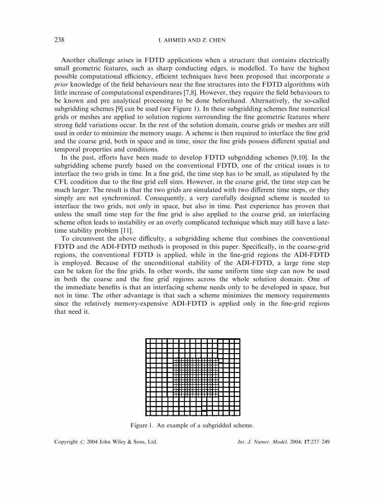
Another challenge arises in FDTD applications when a structure that contains electricallysmall geometric features, such as sharp conducting edges, is modelled. To have the highestpossible computational efficiency, efficient techniques have been proposed that incorporate aprior knowledge of the field behaviours near the fine structures into the FDTD algorithms withlittle increase of computational expenditures [7,8]. However, they require the field behaviours tobe known and pre analytical processing to be done beforehand. Alternatively, the so-calledsubgridding schemes [9] can be used (see Figure 1). In these subgridding schemes fine numericalgrids or meshes are applied to solution regions surrounding the fine geometric features wherestrong field variations occur. In the rest of the solution domain, coarse grids or meshes are stillused in order to minimize the memory usage. A scheme is then required to interface the fine gridand the coarse grid, both in space and in time, since the fine grids possess different spatial andtemporal properties and conditions.

In the past, efforts have been made to develop FDTD subgridding schemes [9,10]. In thesubgridding scheme purely based on the conventional FDTD, one of the critical issues is tointerface the two grids in time. In a fine grid, the time step has to be small, as stipulated by theCFL condition due to the fine grid cell sizes. However, in the coarse grid, the time step can bemuch larger. The result is that the two grids are simulated with two different time steps, or theysimply are not synchronized. Consequently, a very carefully designed scheme is needed tointerface the two grids, not only in space, but also in time. Past experience has proven thatunless the small time step for the fine grid is also applied to the coarse grid, an interfacingscheme often leads to instability or an overly complicated technique which may still have a late-time stability problem [11].

To circumvent the above difficulty, a subgridding scheme that combines the conventionalFDTD and the ADI-FDTD methods is proposed in this paper. Specifically, in the coarse-gridregions, the conventional FDTD is applied, while in the fine-grid regions the ADI-FDTDis employed. Because of the unconditional stability of the ADI-FDTD, a large time stepcan be taken for the fine grids. In other words, the same uniform time step can now be usedin both the coarse and the fine grid regions across the whole solution domain. One ofthe immediate benefits is that an interfacing scheme needs only to be developed in space, butnot in time. The other advantage is that such a scheme minimizes the memory requirementssince the relatively memory-expensive ADI-FDTD is applied only in the fine-grid regionsthat need it.

Figure 1. An example of a subgridded scheme.

Copyright # 2004 John Wiley & Sons, Ltd. Int. J. Numer. Model. 2004; 17:237–249

I. AHMED AND Z. CHEN238

In the following sections, the hybrid FDTD and ADI-FDTD subgridding schemes are firstintroduced in both 2D and 3D cases. They are compared with the pure FDTD modelling for afinned waveguide, an insulated fin line structure and a cavity.

2. TWO-DIMENSIONAL INTERFACE

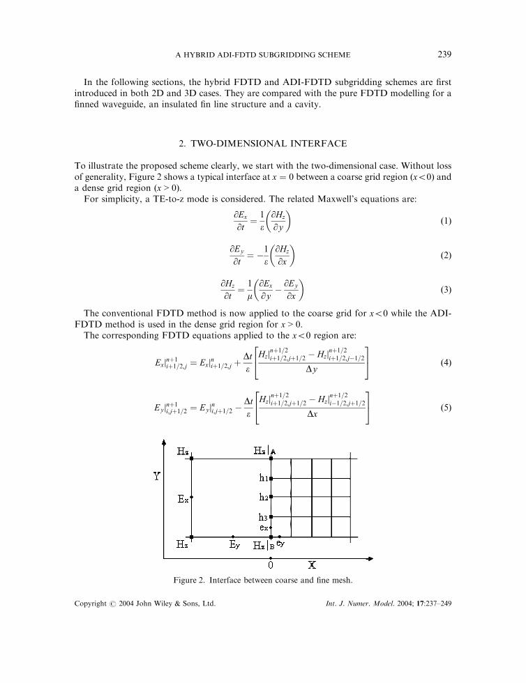
To illustrate the proposed scheme clearly, we start with the two-dimensional case. Without lossof generality, Figure 2 shows a typical interface at x ¼ 0 between a coarse grid region ðx50Þ anda dense grid region ðx > 0Þ:

For simplicity, a TE-to-z mode is considered. The related Maxwell’s equations are:

@Ex

@t¼

1

e@Hz

@y

� �ð1Þ

@Ey

@t¼ �

1

e@Hz

@x

� �ð2Þ

@Hz

@t¼

1

m@Ex

@y�

@Ey

@x

� �ð3Þ

The conventional FDTD method is now applied to the coarse grid for x50 while the ADI-FDTD method is used in the dense grid region for x > 0:

The corresponding FDTD equations applied to the x50 region are:

Exjnþ1iþ1=2;j ¼ Exj

niþ1=2;j þ

Dte

Hzjnþ1=2iþ1=2;jþ1=2 � Hzj

nþ1=2iþ1=2;j�1=2

Dy

24

35 ð4Þ

Ey jnþ1i;jþ1=2 ¼ Ey jni;jþ1=2 �

Dte

Hzjnþ1=2iþ1=2;jþ1=2 � Hzj

nþ1=2i�1=2;jþ1=2

Dx

24

35 ð5Þ

Figure 2. Interface between coarse and fine mesh.


A HYBRID ADI-FDTD SUBGRIDDING SCHEME 239

Hzjnþ1=2iþ1=2;jþ1=2 ¼Hzj

n�1=2iþ1=2;jþ1=2 þ

Dtm

Exjniþ1=2;jþ1 � Exjniþ1=2;j

Dy

� �

�Dtm

Ey jniþ1;jþ1=2 � Ey j

ni;jþ1=2

Dx

� �ð6Þ

where n indicates the nth time step, and i and j correspond to the position ðx ¼ iDx; y ¼ jDyÞ: Dxand Dy are the space increments in the x and y directions in the coarse grid region ðx50Þ:

The corresponding ADI-FDTD equations applied to the x > 0 region are:


niþ1=2;j þ

Dte

Hzjnþ1iþ1=2;jþ1=2 � Hzjnþ1

iþ1=2;j�1=2

Dy0

" #ð7Þ

Ey jnþ1i;jþ1=2 ¼ Ey j

ni;jþ1=2 �

Dte

Hzjniþ1=2;jþ1=2 � Hzjni�1=2;jþ1=2

Dx0

� �ð8Þ

Hzjnþ1iþ1=2;jþ1=2 ¼Hzj

niþ1=2;jþ1=2 þ

Dtm

Exjnþ1iþ1=2;jþ1 � Exjnþ1

iþ1=2;j

Dy0 �Ey jniþ1;jþ1=2 � Ey jni;jþ1=2

Dx0

" #ð9Þ

for the first sub-step, and


nþ1iþ1=2;j þ

Dte


iþ1=2;j�1=2

Dy0

" #ð10Þ

Ey jnþ2i;jþ1=2 ¼ Ey j

nþ1i;jþ1=2 �

Dte


i�1=2;jþ1=2

Dx0

" #ð11Þ

Hzjnþ2iþ1=2;jþ1=2 ¼Hzj

nþ1iþ1=2;jþ1=2 þ

Dtm

Exjnþ1iþ1=2;jþ1 � Exjnþ1

iþ1=2;j

Dy0 �Ey jnþ2

iþ1;jþ1=2 � Ey jnþ2i;jþ1=2

Dx0

" #ð12Þ

for the second sub-step.Note that in the ADI-FDTD equations (7)–(12), Dx0 and Dy0 are the space increments in the x

and y directions in the dense grid region ðx > 0Þ: They are different from the space increments,Dx and Dy of Equations (4)–(6), in the coarse grid region ðx50Þ:

In order to synchronize the simulations between the FDTD and the ADI-FDTD, the timestep for the ADI-FDTD is taken the same as for the conventional FDTD. Thus, one single fullADI-FDTD iteration amounts to two FDTD iterations. In doing so, the interpolation of thefields at the interface ðx ¼ 0Þ between the FDTD and ADI-FDTD grids need to be carried outonly in space. An example is shown in Figure 2, where the field quantity to be interpolatedbetween the dense and coarse grids is Hz: A simple linear interpolation scheme is then employed.More specifically, the in-between values of Hz; denoted as h1; h2 and h3; can be obtained asfollows:

h1 ¼ 34HzjA þ

14HzjB ð13Þ

h2 ¼ 12HzjA þ

12HzjB ð14Þ

h3 ¼ 14HzjA þ

34HzjB ð15Þ



Note that in Figure 2, it is assumed that the dense grid is four times denser than the coarsegrid. The above equations are applied to the case where the dense to coarse grid size ratio isfour. For a general ratio of m; the above equation can be easily written as

hl ¼m� lm

HzjA þlmHzjB ð16Þ

where hl; l ¼ 1; 2; . . . ;m� 1; are the field values to be interpolated in between points A and B:It should be pointed out here that the relatively large time-step applied in the dense grid will

not cause unacceptable numerical dispersion errors as long as the time step does not causeunacceptable errors in the coarse grid. This is because the ADI-FDTD and FDTD presentsimilar dispersion errors if their time and spatial step sizes are comparable [12]. In our case, theADI-FDTD actually has a smaller grid size than the FDTD. Therefore, the numericaldispersion error in the dense grid should not be larger than the coarse grid.

3. THREE-DIMENSIONAL INTERFACE

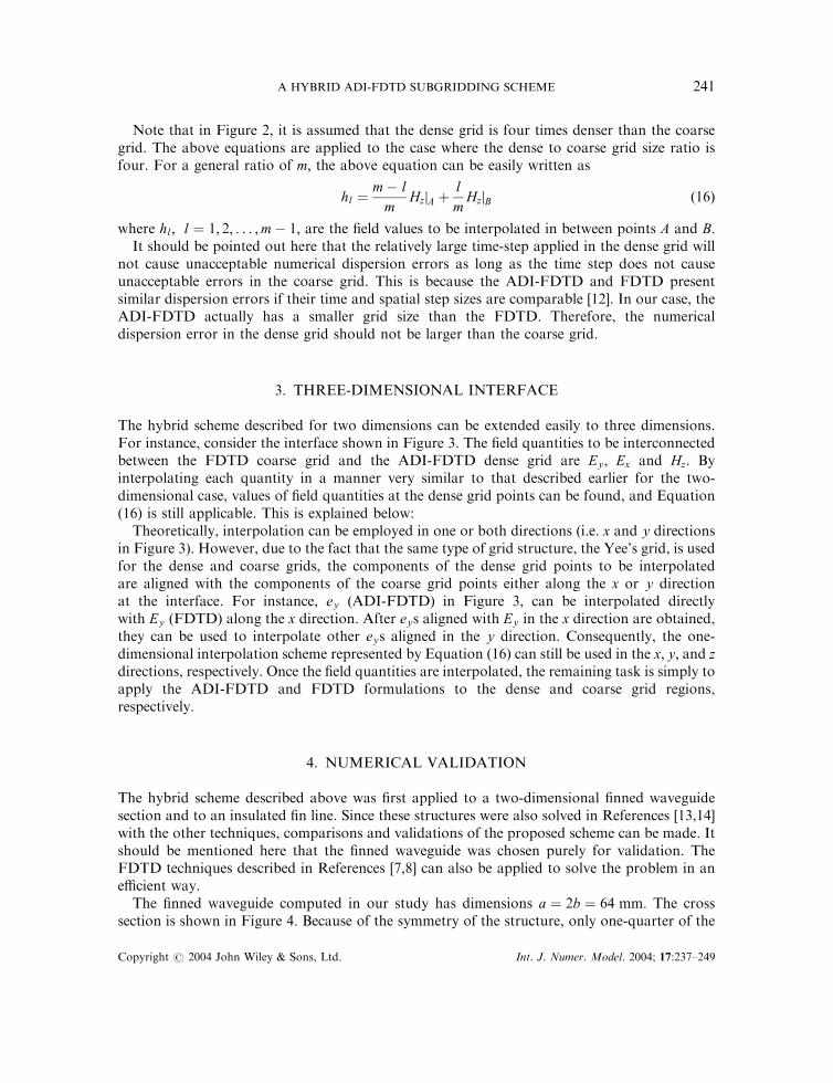
The hybrid scheme described for two dimensions can be extended easily to three dimensions.For instance, consider the interface shown in Figure 3. The field quantities to be interconnectedbetween the FDTD coarse grid and the ADI-FDTD dense grid are Ey ; Ex and Hz: Byinterpolating each quantity in a manner very similar to that described earlier for the two-dimensional case, values of field quantities at the dense grid points can be found, and Equation(16) is still applicable. This is explained below:

Theoretically, interpolation can be employed in one or both directions (i.e. x and y directionsin Figure 3). However, due to the fact that the same type of grid structure, the Yee’s grid, is usedfor the dense and coarse grids, the components of the dense grid points to be interpolatedare aligned with the components of the coarse grid points either along the x or y directionat the interface. For instance, ey (ADI-FDTD) in Figure 3, can be interpolated directlywith Ey (FDTD) along the x direction. After eys aligned with Ey in the x direction are obtained,they can be used to interpolate other eys aligned in the y direction. Consequently, the one-dimensional interpolation scheme represented by Equation (16) can still be used in the x; y; and zdirections, respectively. Once the field quantities are interpolated, the remaining task is simply toapply the ADI-FDTD and FDTD formulations to the dense and coarse grid regions,respectively.

4. NUMERICAL VALIDATION

The hybrid scheme described above was first applied to a two-dimensional finned waveguidesection and to an insulated fin line. Since these structures were also solved in References [13,14]with the other techniques, comparisons and validations of the proposed scheme can be made. Itshould be mentioned here that the finned waveguide was chosen purely for validation. TheFDTD techniques described in References [7,8] can also be applied to solve the problem in anefficient way.

The finned waveguide computed in our study has dimensions a ¼ 2b ¼ 64 mm: The crosssection is shown in Figure 4. Because of the symmetry of the structure, only one-quarter of the



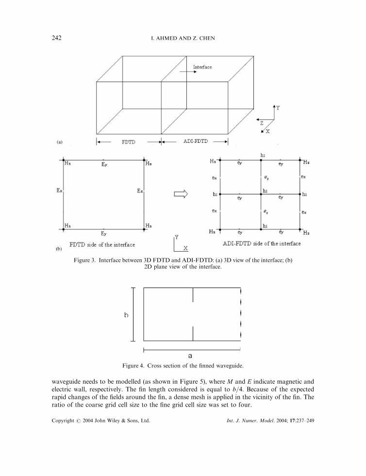
waveguide needs to be modelled (as shown in Figure 5), where M and E indicate magnetic andelectric wall, respectively. The fin length considered is equal to b=4: Because of the expectedrapid changes of the fields around the fin, a dense mesh is applied in the vicinity of the fin. Theratio of the coarse grid cell size to the fine grid cell size was set to four.

Figure 3. Interface between 3D FDTD and ADI-FDTD: (a) 3D view of the interface; (b)2D plane view of the interface.

Figure 4. Cross section of the finned waveguide.



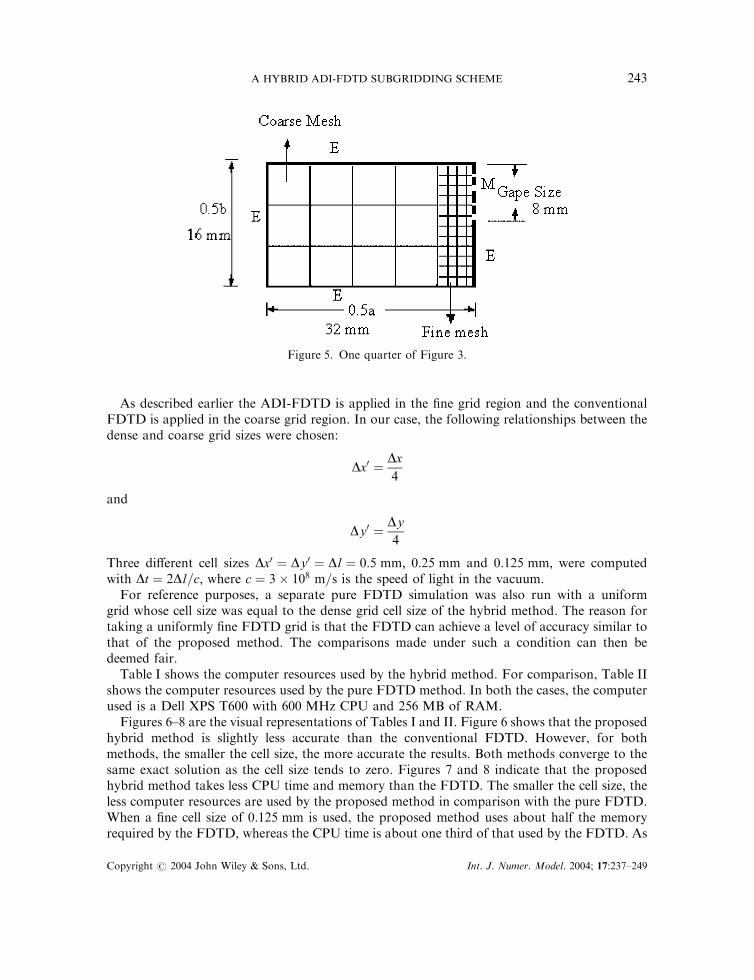
As described earlier the ADI-FDTD is applied in the fine grid region and the conventionalFDTD is applied in the coarse grid region. In our case, the following relationships between thedense and coarse grid sizes were chosen:

Dx0 ¼Dx4

and

Dy0 ¼Dy4

Three different cell sizes Dx0 ¼ Dy0 ¼ Dl ¼ 0:5 mm; 0:25 mm and 0:125 mm; were computedwith Dt ¼ 2Dl=c; where c ¼ 3� 108 m=s is the speed of light in the vacuum.

For reference purposes, a separate pure FDTD simulation was also run with a uniformgrid whose cell size was equal to the dense grid cell size of the hybrid method. The reason fortaking a uniformly fine FDTD grid is that the FDTD can achieve a level of accuracy similar tothat of the proposed method. The comparisons made under such a condition can then bedeemed fair.

Table I shows the computer resources used by the hybrid method. For comparison, Table IIshows the computer resources used by the pure FDTD method. In both the cases, the computerused is a Dell XPS T600 with 600 MHz CPU and 256 MB of RAM.

Figures 6–8 are the visual representations of Tables I and II. Figure 6 shows that the proposedhybrid method is slightly less accurate than the conventional FDTD. However, for bothmethods, the smaller the cell size, the more accurate the results. Both methods converge to thesame exact solution as the cell size tends to zero. Figures 7 and 8 indicate that the proposedhybrid method takes less CPU time and memory than the FDTD. The smaller the cell size, theless computer resources are used by the proposed method in comparison with the pure FDTD.When a fine cell size of 0:125 mm is used, the proposed method uses about half the memoryrequired by the FDTD, whereas the CPU time is about one third of that used by the FDTD. As

Figure 5. One quarter of Figure 3.



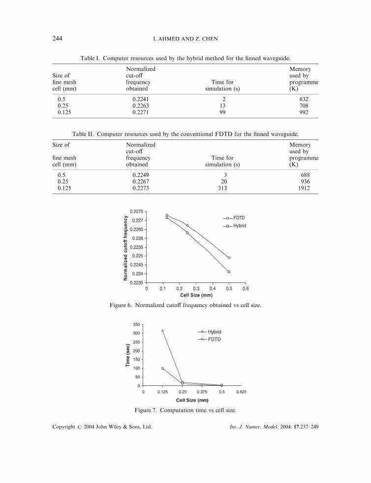
Table I. Computer resources used by the hybrid method for the finned waveguide.

Normalized MemorySize of cut-off used byfine mesh frequency Time for programmecell (mm) obtained simulation (s) (K)

0.5 0.2241 2 6320.25 0.2263 13 7080.125 0.2271 99 992

Table II. Computer resources used by the conventional FDTD for the finned waveguide.

Size of Normalized Memorycut-off used by

fine mesh frequency Time for programmecell (mm) obtained simulation (s) (K)

0.5 0.2249 3 6880.25 0.2267 20 9360.125 0.2273 313 1912

0.2235

0.224

0.2245

0.225

0.2255

0.226

0.2265

0.227

0.2275

0 0.1 0.2 0.3 0.4 0.5 0.6

No

rmal

ized

cu

toff

fre

qu

ency FDTD

Hybrid

Cell Size (mm)

Figure 6. Normalized cutoff frequency obtained vs cell size.

0

50

100

150

200

250

300

350

0 0.125 0.25 0.375 0.5 0.625

Cell Size (mm)

Tim

e (s

ec)

Hybrid

FDTD

Figure 7. Computation time vs cell size.



a result, we conclude that the proposed hybrid method is superior to the pure FDTD methodwhen a fine grid is required.

Another two dimensional structure that was simulated with the hybrid method is an insulatedfin line structure. Its geometry is the same as that of the finned waveguide except for the additionof insulation around the fin (Figure 9). Again, for reference, a separate FDTD computation wasdone with a uniform grid whose cell size is equal to the dense grid cell size of the hybrid method.In the simulations with the hybrid method, the coarse grid cell size, Dx ¼ Dy; is fixed at 1 mm;while the fine grid cell size, Dx0 ¼ Dy0; is varied from 1 to 0:25 mm: The simulation results areshown in Figure 10. These results indicate the differences in cutoff frequencies computed withboth the hybrid method and the FDTD method, for increasing insulation width. As can be seen,differences between the two methods are small and decrease as the width increases.

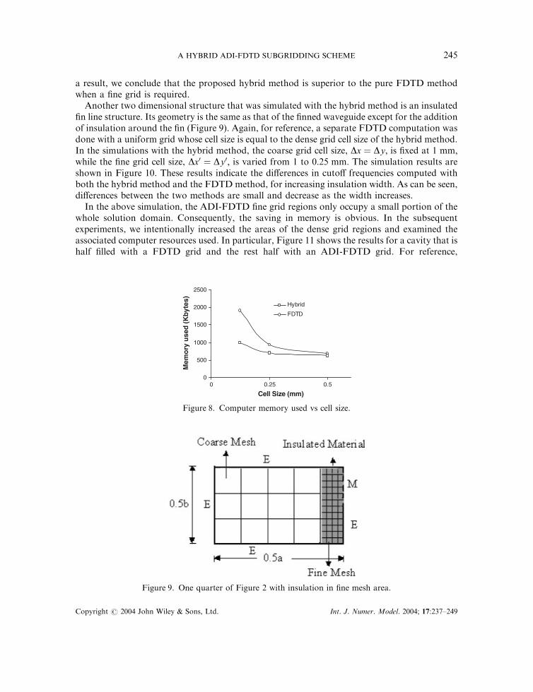
In the above simulation, the ADI-FDTD fine grid regions only occupy a small portion of thewhole solution domain. Consequently, the saving in memory is obvious. In the subsequentexperiments, we intentionally increased the areas of the dense grid regions and examined theassociated computer resources used. In particular, Figure 11 shows the results for a cavity that ishalf filled with a FDTD grid and the rest half with an ADI-FDTD grid. For reference,

0

500

1000

1500

2000

2500

0 0.25 0.5

Cell Size (mm)

Mem

ory

use

d (

Kb

ytes

)

Hybrid

FDTD

Figure 8. Computer memory used vs cell size.

Figure 9. One quarter of Figure 2 with insulation in fine mesh area.



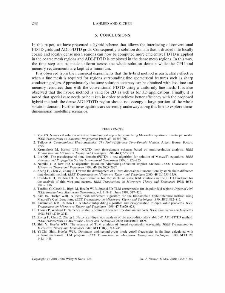
a separate FDTD simulation was run again with its cell size equal to the fine grid size employedfor the hybrid method. The cavity size was 16 mm� 8 mm: The coarse grid cell size was fixed at1 mm while the dense grid cell size was varied with different ratios of coarse to dense gridcell sizes.

Figure 11(a) shows the layout of the grid for the cavity with the proposed hybrid method.Figure 11(b) shows the relative errors when different cell size ratios were used. Figure 11(c)presents memory used by the hybrid method and the FDTD method versus grid size ratios.Figure 11(d) presents the CPU time used by the two methods with different grid size ratios.Based on these figures, the following observations are made:

(A) In the hybrid method, as the coarse to dense grid size ratio increases, the computationerror decreases.

(B) Memory used by the hybrid method is slightly higher than that required by the FDTD.In other words, when the dense ADI-FDTD grid occupies 50% of the solution domain,the memory used by the hybrid method starts to be larger than that used by the FDTDalone. This is due to the fact that the ADI-FDTD method computes more componentsthan the FDTD method.

(C) Although the hybrid method starts to use more memory, the CPU time required by theproposed hybrid method is still less than that of the FDTD, especially in the case of largegrid size ratios.

In all, it is concluded that the proposed hybrid method is effective and efficient for numericalsubgridding, provided subgridding regions do not occupy a large portion of the solutiondomain. In the 2D case, they should not exceed 50% of the domain.

A three-dimensional case involving a cavity with dimensions of 8 mm� 8 mm� 8 mmwas also computed since an analytical solution is readily available. One-half of the cavityis filled with the coarse FDTD grid, while the other half is filled with the dense ADI-FDTDgrid. The results are shown in Table III (for a grid size ratio of 1:2 and a coarse grid cellsize (FDTD) of 0:333 mm). It can be observed that the error of the hybrid method isbelow 0.88%. This indicates that the proposed hybrid method is also effective in the three-dimensional case.

0.165

0.17

0.175

0.18

0.185

0.19

0.195

0.2

0.205

0 2 4 6 8 10width of Insulated material (mm)

No

rmal

ized

cu

toff

freq

uen

cy

Hybrid

FDTD

Figure 10. Normalized cutoff frequency obtained vs width of insulator material.



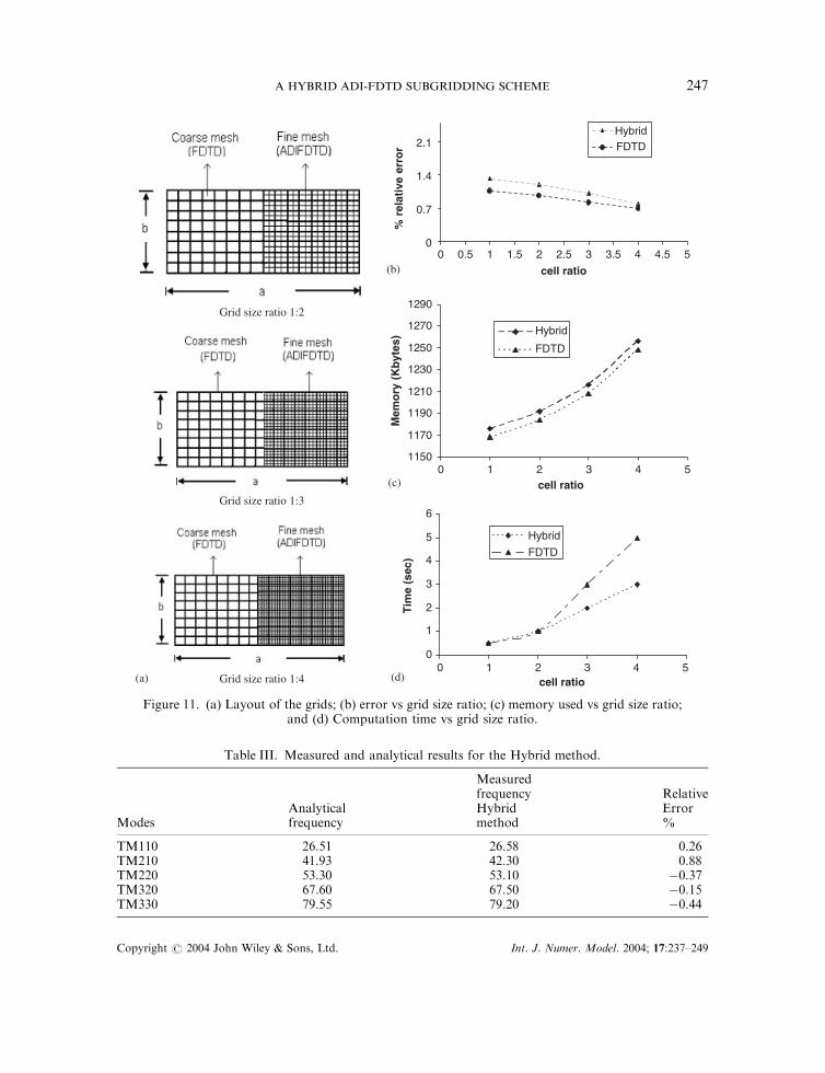
Table III. Measured and analytical results for the Hybrid method.

Measuredfrequency Relative

Analytical Hybrid ErrorModes frequency method %

TM110 26.51 26.58 0.26TM210 41.93 42.30 0.88TM220 53.30 53.10 �0.37TM320 67.60 67.50 �0.15TM330 79.55 79.20 �0.44

1150

1170

1190

1210

1230

1250

1270

1290

0 1 2 3 4 5cell ratio

Mem

ory

(K

byt

es)

0

0.7

1.4

2.1

0 1.5 2.5 3 4.540.5 1 2 3.5 5

cell ratio

% r

elat

ive

erro

r

Hybrid

FDTD

0

1

2

3

4

5

6

0 1 2 3 4 5cell ratio

Tim

e (s

ec)

Hybrid

FDTD

HybridFDTD

(b)

(c)

(d)(a)

Grid size ratio 1:2

Grid size ratio 1:3

Grid size ratio 1:4

Figure 11. (a) Layout of the grids; (b) error vs grid size ratio; (c) memory used vs grid size ratio;and (d) Computation time vs grid size ratio.



5. CONCLUSIONS

In this paper, we have presented a hybrid scheme that allows the interfacing of conventionalFDTD grids and ADI-FDTD grids. Consequently, a solution domain that is divided into locallycoarse and locally dense mesh regions can now be computed more efficiently; FDTD is appliedin the coarse mesh regions and ADI-FDTD is employed in the dense mesh regions. In this way,the time step can be made uniform across the whole solution domain while the CPU andmemory requirements are kept at a minimum.

It is observed from the numerical experiments that the hybrid method is particularly effectivewhen a fine mesh is required for regions surrounding fine geometrical features such as sharpconducting edges. Approximately the same solution accuracy can be obtained with less time andmemory resources than with the conventional FDTD using a uniformly fine mesh. It is alsoobserved that the hybrid method is valid for 2D as well as for 3D applications. Finally, it isnoted that special care needs to be taken in order to achieve better efficiency with the proposedhybrid method: the dense ADI-FDTD region should not occupy a large portion of the wholesolution domain. Further investigations are currently underway along this line to explore three-dimensional modelling scenarios.

REFERENCES

1. Yee KS. Numerical solution of initial boundary value problems involving Maxwell’s equations in isotropic media.IEEE Transactions on Antennas Propagation 1966; AP-14:302–307.

2. Taflove A. Computational Electrodynamics: The Finite-Difference Time-Domain Method. Artech House: Boston,1995.

3. Krumpholz M, Katehi LPB. MRTD: new time-domain schemes based on multiresolution analysis. IEEETransactions on Microwave Theory and Techniques 1996; 44(4):555–571.

4. Liu QH. The pseudospectral time domain (PSTD): a new algorithm for solution of Maxwell’s equations. IEEEAntennas and Propagation Society International Symposium 1997; 1:122–125.

5. Namiki T. A new FDTD algorithm based on Alternating-Direction Implicit Method. IEEE Transactions onMicrowave Theory and Techniques 1999; 47(10):2003–2007.

6. Zheng F, Chen Z, Zhang J. Toward the development of a three-dimensional unconditionally stable finite-differencetime-domain method. IEEE Transactions on Microwave Theory and Techniques 2000; 48(9):1550–1558.

7. Craddock IJ, Railton CJ. A new technique for the stable of static field solutions in the FDTD method forthe analysis of thin wire and narrow. IEEE Transactions on Microwave Theory and Techniques 1998; 46(8):1091–1096.

8. Tardioli G, Cascio L, Righi M, Hoefer WJR. Special 3D-TLM corner nodes for singular field regions. Digest of 1997IEEE International Microwave Symposium, vol. 1, 8–11, June 1997; 317–320.

9. Kim IS, Hoefer WJR. A local mesh refinement algorithm for the time-domain finite-difference method usingMaxwell’s Curl Equations. IEEE Transactions on Microwave Theory and Techniques 1990; 38(6):812–815.

10. Krishnaiah KM, Railton CJ. A Stable subgridding algorithm and its application to eigen value problems. IEEETransactions on Microwave Theory and Techniques 1999; 47(5):620–628.

11. Thoma P, Weiland T. Numerical stability of finite difference time domain methods. IEEE Transactions on Magnetics1998; 34(5):2740–2743.

12. Zheng F, Chen Z, Zhang J. Numerical dispersion analysis of the unconditionally stable 3-D ADI-FDTD method.IEEE Transactions on Microwave Theory and Techniques 2001; 49(5):1006–1009.

13. Shih Y, Hoefer WJR. The accuracy of TLM analysis of finned rectangular waveguide. IEEE Transactions onMicrowave Theory and Techniques 1980; MTT 28(7):743–746.

14. Yi-Chi- Shih, Hoefer WJR. Dominant and second-order mode cutoff frequencies in fin lines calculated witha two-dimensional TLM program. IEEE Transactions on Microwave Theory and Techniques 1980; MTT 28:1443–1448.



AUTHORS’ BIOGRAPHIES

Iftikhar Ahmed (S’02) received the BSc Electrical Engineering degree from theUniversity of Engineering and Technology Taxila, Pakistan, in 1995, the MScElectrical Engineering degree from University of engineering and Technology Lahore,Pakistan, in 1999, and is currently working toward the PhD degree in ElectricalEngineering at Dalhousie University, Halifax, NS, Canada.

His research interests include computational electromagnetics, RF circuit design,numerical modelling of RF/Microwave structures, and wireless communicationsystem design.

Zhizhang (David) Chen (S’92-M’92-SM’96) received the BEng degree from FuzhouUniversity, Fuzhou, China, in 1982, the MASc degree from Southeast University,Nanjing, China, in 1986, and the PhD degree from the University of Ottawa, Ottawa,ON, Canada, in 1992.

From January of 1993 to August of 1993, he was a Natural Science andEngineering Research Council Post-Doctoral Fellow with the Department ofElectrical and Computer Engineering, McGill University, Montreal, QC, Canada.In 1993, he joined the Department of Electrical and Computer Engineering,Dalhousie University, Halifax, NS, Canada, where he is currently a Professor. He hasauthored and coauthored over 100 journal and conference papers, as well asindustrial reports in the areas of computational electromagnetics and RF/microwaveelectronics for wireless communications. His current research interests include RF/microwave electronics, numerical modelling and simulation, and antenna designs forwireless and satellite communications.



a hybrid adi-fdtd subgridding scheme for efficient electromagnetic computation

Documents