a history of cepstrum analysis and its application to...
TRANSCRIPT

1
A History of Cepstrum Analysis and its
Application to Mechanical Problems
Robert B Randall1
1 School of Mechanical and Manufacturing Engineering
University of New South Wales, Sydney 2052, Australia
Abstract It is not widely realised that the first paper on cepstrum analysis was published two years before the FFT
algorithm, despite having Tukey as a common author, and its definition was such that it was not reversible
even to the log spectrum. After publication of the FFT in 1965, the cepstrum was redefined so as to be
reversible to the log spectrum, and shortly afterwards Oppenheim and Schafer defined the “complex
cepstrum”, which was reversible to the time domain. They also derived the analytical form of the complex
cepstrum of a transfer function in terms of its poles and zeros. The cepstrum had been used in speech
analysis for determining voice pitch (by accurately measuring the harmonic spacing), but also for separating
the formants (transfer function of the vocal tract) from voiced and unvoiced sources, and this led quite early
to similar applications in mechanics. The first was to gear diagnostics (Randall), where the cepstrum greatly
simplified the interpretation of the sideband families associated with local faults in gears, and the second was
to extraction of diesel engine cylinder pressure signals from acoustic response measurements (Lyon and
Ordubadi). Later Polydoros defined the differential cepstrum, which had an analytical form similar to the
impulse response function, and Gao and Randall used this and the complex cepstrum in the application of
cepstrum analysis to modal analysis of mechanical structures. Antoni proposed the mean differential
cepstrum, which gave a smoothed result. The cepstrum can be applied to MIMO systems if at least one
SIMO response can be separated, and a number of blind source separation techniques have been proposed for
this. Most recently it has been shown that even though it is not possible to apply the complex cepstrum to
stationary signals, it is possible to use the real cepstrum to edit their (log) amplitude spectrum, and combine
this with the original phase to obtain edited time signals. This has already been used for a wide range of
mechanical applications.
1 Introduction
The first paper on cepstrum analysis [1] defined it as “the power spectrum of the logarithm of the power
spectrum”. The original application was to the detection of echoes in seismic signals, where it was shown to
be greatly superior to the autocorrelation function, because it was insensitive to the colour of the signal. This
purely diagnostic application did not require returning to the log spectrum, and the reason for the definition
was presumably that software for producing power spectra was readily available. Even though [1] had one of
the authors of the FFT algorithm (John Tukey) as a co-author it was published two years before the FFT
algorithm [2] and thus the potential of the latter was not yet realised. Tukey himself in [1] writes “Although
spectral techniques, involving second-degree operations, are now quite familiar, the apparently simpler first-
degree Fourier techniques are less well known” (he then refers to a paper of which he is the sole author,
which confirms that he made the remark). Thus, the original cepstrum was not reversible even to the log
spectrum, and so even though the word and concept of a “lifter” (a filter in the cepstrum) was defined in the
original paper, this was enacted as a convolutive filter applied to the log spectrum rather than a window in
the cepstrum. The diagnostic application was also satisfactory for determining the voice pitch of voiced
speech [3], so speech analysis was one of the earliest applications, much of the development being done at
Bell Telephone Labs.
The early history of the development of the cepstrum was recently published by the two pioneers
Oppenheim and Schafer [4], but their paper primarily covers applications in speech analysis,

2
communications, seismology and geophysics, and no mechanical applications are given. They describe how
Oppenheim’s PhD dissertation at MIT [5] introduced the concept of “homomorphic systems”, where
nonlinear relationships could be converted into linear ones to allow linear filtering in the transform domain.
Typical examples were conversion of multiplication into addition by the log operation, and conversion of
convolution by first applying the Fourier transform (to convert the convolution to a multiplication) followed
by the logarithmic conversion. It was a small further step to perform a (linear) inverse Fourier transform on
the log spectrum to obtain a new type of cepstrum, and this was the basis of Schafer’s PhD dissertation at
MIT [6]. By retaining the phase in all operations, the “complex cepstrum” was defined as the inverse Fourier
transform of the complex logarithm of the complex spectrum, and this was thus reversible to the time
domain. Oppenheim and Schafer collaborated on a book [7], in which a number of further developments and
applications of the cepstrum were reported, in particular the analytical form of the cepstrum for sampled
signals, where the Fourier transform could be replaced by the z-transform.
2 Basic Relationships and Definitions
2.1 Formulations
The original definition of the (power) cepstrum was:
(1)
where ( )xxF f is a power spectrum, which can be an averaged power spectrum or the amplitude squared
spectrum of a single record.
The definition of the complex cepstrum is:
(2)
where ( )( ) ( ) ( ) j fF f f t A f e (3)
in terms of the amplitude and phase of the spectrum. It is worth noting that the “complex cepstrum” is
real, despite its name, because the log amplitude of the spectrum is even, and the phase spectrum is odd.
The new power cepstrum is given by:
(4)
which for the spectrum of a single record (as in (3)) can be expressed as:
(5)
The so-called real cepstrum is obtained by setting the phase to zero in Eq. (2):
(6)
which is seen to be simply a scaled version of (5).
It should be noted that the complex cepstrum requires the phase ( )f to be unwrapped to a continuous
function of frequency, and this places a limit on its application. It cannot be used for example with stationary
signals, made up of discrete frequency components (where the phase is undefined at intermediate frequencies)
and stationary random components (where the phase is random). This point is taken up later. It can only be
used with well-behaved functions such as impulse responses, where the phase is well-defined (and often
related to the log amplitude). The unwrapping can usually be accomplished using an algorithm such as
UNWRAP in Matlab, although the latter may give errors where the slope of the phase function is steep.
This problem can usually be resolved by repeatedly interpolating the spectra by factors of 2 until the same
2
( ) log ( )p xxC F f
1 1( ) log ( ) ln ( ) ( )cC F f A f j f
1( ) log ( )p xxC F f
1( ) 2ln ( )pC A f
1( ) ln ( )rC A f

3
result is obtained with successive steps. The penultimate step can then be used. Errors in unwrapping can
also occur when the amplitude is very small, so that noise affects the phase estimates.
As mentioned above, Oppenheim and Schafer in [7] derived the analytical formulation of the cepstrum
for transfer functions, from digitised signals, expressed using the z-transform in terms of their poles and
zeros in the z-plane. Thus, for a general impulse response function:
(7)
where the Ai are residues, si and zi poles in the s-plane and z-plane, respectively, and t the time sample
spacing, the transfer function in the z-plane is given by:
(8)
where the ci and ai are poles and zeros inside the unit circle in the z-plane, respectively, and the di and
bi are the (reciprocals of the) poles and zeros outside the unit circle, respectively (so that
, , , 1i i i ia b c d ). Oppenheim and Schafer [7] show that for this transfer function ( )H z , the cepstrum
can be represented as:
(9)
Here, n is time sample number, known as “quefrency” (see Section 2.2). It will be seen that the poles and
zeros inside the unit circle, which define the minimum phase part of the transfer function, have a causal
cepstrum, with positive quefrency components only, while the poles and zeros outside the unit circle,
defining the maximum phase part, form the cepstrum at negative quefrency. Oppenheim and Schafer thus
were able to demonstrate that the real and imaginary parts of the Fourier transform of the cepstrum of a
minimum phase function (the log amplitude and phase spectra, respectively) are Hilbert transforms of each
other. Hence, if it is known that a transfer function is minimum phase (often the case for many simple
mechanical structures), it is not necessary to measure or unwrap the phase, as it can be calculated from the
log amplitude. In fact, the easiest way to do this is to form the complex cepstrum (one-sided) from the real
cepstrum (real and even) by doubling positive quefrency components and setting negative quefrency
components to zero. The log amplitude and phase spectra can then be obtained by a forward transform of the
complex cepstrum.
One further property of the cepstrum, already mentioned as a homomorphic property, was developed
quite early, and that is that forcing function and transfer function effects are additive in the cepstrum. For
SIMO (single input, multiple output) systems, any output signal is the convolution of the input signal with
the impulse response function of the transmission path, and this convolutive relationship is converted to an
addition by the cepstrum operation as follows:
If ( ) ( ) ( )y t f t h t (10)
then ( ) ( ) ( )Y f F f H f (11)
log ( ) log ( ) log ( )Y f F f H f (12)
2 2
1 1
( ) i
N Ns n t n
i i i
i i
h n A e A z
1
1 1
1
1 1
(1 ) (1 )
( )
(1 ) (1 )
i o
i o
M M
i i
i i
N N
i i
i i
B a z b z
H z
c z d z
( ) ln( ) , 0
( ) , 0
( ) , 0
h
n ni i
h
i i
n ni i
h
i i
C n B n
a cC n n
n n
b dC n n
n n

4
and (13)
Note that this only applies for SIMO systems, since for MIMO (multiple input, multiple output) systems
each response signal is a sum of convolutions. This point is taken up later.
This relationship was used in speech analysis, for example to separate the speech source (voiced or
unvoiced) from the transmission effect of the vocal tract (whose resonances are called “formants”), and in [7]
a vocoder is proposed where the speech information can be considerably compressed by transmitting only
the low quefrency part of the cepstrum (giving the formants) and an indicator of whether the speech segment
is voiced or unvoiced, and if so the voice pitch. To reconstruct the speech, the formants were used to
generate a filter, which was excited either by a noise source (unvoiced) or a periodic pulse generator with
frequency the same as the voice pitch.
2.2 Terminology
In the original paper [1], the authors coined the word “cepstrum” by reversing the first syllable of
“spectrum”, the justification being that it was a “spectrum of a spectrum”. Similarly, the word “quefrency”
was obtained from “frequency”, and the authors also suggested a number of others, including:
rahmonic from harmonic
lifter from filter
gamnitude from magnitude
saphe from phase
darius from radius
dedomulation from demodulation
Of these, cepstrum, quefrency, rahmonic and lifter are useful in clarifying that the operations or features
refer to the cepstrum, rather than the spectrum or time signal, and are still regularly used in the literature, as
well as in this paper. Note that the autocorrelation function is also a “spectrum of a spectrum”, so the
distinctive feature of the cepstrum is the log conversion of the spectrum.
3 Early Applications in Mechanics and Acoustics
3.1 Diagnostics of families of harmonics or sidebands
The author became aware of the possibility of using the cepstrum to detect and quantify families of
periodically spaced spectral components by reading [3] and realised that this would not only detect families
of harmonics, but also equally spaced modulation sidebands. Local faults in gears give an impulsive
modulation of the gearmesh signals (both amplitude and frequency modulation) resulting in large numbers of
sidebands spaced at the speed of the gear on which the local fault is located. The majority of such sidebands
are only visible on a spectrum with a log amplitude scale, and so the cepstrum is an ideal way to collect the
(average) information of a large number of such sidebands into a relatively small number of rahmonics in the
cepstrum, of which the first contains most of the information. He had even experimented with calculating the
cepstrum using FFT methods before joining the company Brüel and Kjær in Copenhagen in 1971. A Fortran
version of the FFT algorithm was obtained from [8]. However, even though B&K had a fully designed mini-
computer-based FFT analyser in 1971, this was never released onto the market, and so other methods of
obtaining the cepstrum were sought. In 1973 an Application Note No. 13-150 entitled “Cepstrum Analysis
and Gearbox Fault Diagnosis” [9] was published by B&K, in which six methods were described for
calculating the (power) cepstrum, primarily for the purpose of diagnosing gear faults. Several were variations
on the theme of using a heterodyne analyser for performing the “frequency” analysis on a linear frequency
scale with constant bandwidth, first to obtain the original power spectrum on a log amplitude scale, and then
the second analysis of the log spectrum to the cepstrum on a linear scale. In between, the log spectrum was
stored in a medium, which could either be a circulating digital memory (a Digital Event Recorder type 7502),
or a tape loop on an FM tape recorder. In both cases the stored spectrum was played back at a much higher
rate than recorded. The initial analysis could either be generated directly from a continuous recording of the
signal on a tape recorder, or sometimes from a recirculated section of signal recorded in a second Digital
1 1 1log ( ) log ( ) log ( )Y f F f H f
5
Event Recorder, possibly using an analogue “Gauss Impulse Multiplier” type 5623, to apply a Gaussian,
rather than Hanning, weighting to the selected and periodically repeated signal section.
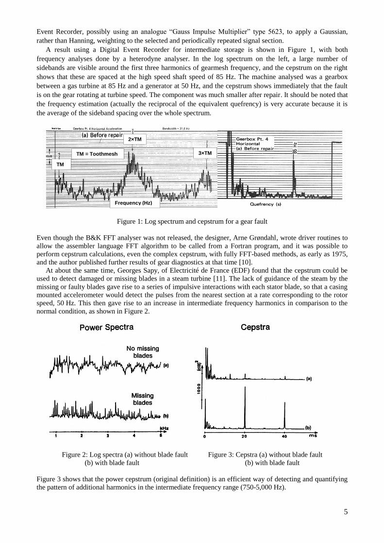
A result using a Digital Event Recorder for intermediate storage is shown in Figure 1, with both
frequency analyses done by a heterodyne analyser. In the log spectrum on the left, a large number of
sidebands are visible around the first three harmonics of gearmesh frequency, and the cepstrum on the right
shows that these are spaced at the high speed shaft speed of 85 Hz. The machine analysed was a gearbox
between a gas turbine at 85 Hz and a generator at 50 Hz, and the cepstrum shows immediately that the fault
is on the gear rotating at turbine speed. The component was much smaller after repair. It should be noted that
the frequency estimation (actually the reciprocal of the equivalent quefrency) is very accurate because it is
the average of the sideband spacing over the whole spectrum.
Figure 1: Log spectrum and cepstrum for a gear fault
Even though the B&K FFT analyser was not released, the designer, Arne Grøndahl, wrote driver routines to
allow the assembler language FFT algorithm to be called from a Fortran program, and it was possible to
perform cepstrum calculations, even the complex cepstrum, with fully FFT-based methods, as early as 1975,
and the author published further results of gear diagnostics at that time [10].
At about the same time, Georges Sapy, of Electricité de France (EDF) found that the cepstrum could be
used to detect damaged or missing blades in a steam turbine [11]. The lack of guidance of the steam by the
missing or faulty blades gave rise to a series of impulsive interactions with each stator blade, so that a casing
mounted accelerometer would detect the pulses from the nearest section at a rate corresponding to the rotor
speed, 50 Hz. This then gave rise to an increase in intermediate frequency harmonics in comparison to the
normal condition, as shown in Figure 2.
Figure 2: Log spectra (a) without blade fault Figure 3: Cepstra (a) without blade fault
(b) with blade fault (b) with blade fault
Figure 3 shows that the power cepstrum (original definition) is an efficient way of detecting and quantifying
the pattern of additional harmonics in the intermediate frequency range (750-5,000 Hz).
Frequency (Hz)
2×TM
3×TM
TM
TM = Toothmesh

6
3.2 Separation of source and transmission path
One of the first groups to apply the cepstrum to the separation of forcing function and transfer function in
mechanical systems was Professor Richard Lyon of MIT, and co-workers. With his doctoral student Afarin
Ordubadi he showed how the complex cepstrum could be used to extract the cylinder pressure (source)
signal from measured acoustic responses [12]. Figure 4 shows the estimated pressure signals from two
cylinders of a diesel engine from this paper.
Figure 4: Estimated cylinder pressure using the complex cepstrum [12]
In 1984, the author proposed using the cepstrum for separating the gearmesh forcing function (single
input) from the structural transfer function in a gearbox [13]. This was considered important because for
example an increase in the second harmonic of the gearmesh frequency might be due to tooth wear (normally
in two patches on each tooth, one on each side of the pitchline, where there is a rolling rather than sliding
action). However, it might be because a natural frequency of the structure or internals has reduced so as to
coincide with the harmonic in question because of a developing crack, and this situation might have a very
different prognosis. Figure 5 shows an example [14] based on this idea, where the periodic forcing function
of the gearmesh was removed in the cepstrum using a comb lifter adjusted to the gearmesh quefrency,
leaving a cepstrum dominated by the transfer function to the measurement point. The edited cepstrum was
transformed back to the log spectrum, which shows that the latter was little changed for two measurements
on the same gearbox, where one had the presence of cracked teeth. Even though a modal analysis was not
carried out, it is obvious that the natural frequencies did not change appreciably.
Figure 5: Use of liftering in the cepstrum to remove the forcing function component from the cepstra for
a gear with and without cracked teeth, leaving the part dominated by the structural transfer functions [14]

7
4 Later Developments up to the Present
4.1 Applications of the real cepstrum in machine diagnostics
From 1975 to 1980, the author made a number of further developments to the application of the real
cepstrum to gear diagnostics, presented at a number of conferences, and which culminated in the publication
of a second Application Note with the same title as [9], published by B&K in 1980, but also in the journal
Maintenance Management International [15]. In this, a number of practical considerations in the calculation
and interpretation of the cepstrum are discussed, of which perhaps the most important is the recommendation
to use the amplitude of the “analytic cepstrum” in place of the normal definition of the real or power
cepstrum, in particular when it is based on a section of the spectrum not starting from zero frequency (eg a
zoom spectrum) or when sidebands are not simultaneously a harmonic series passing through zero frequency
(as can happen with planetary gears because the sun speed is not a subharmonic of the mesh frequency). In
this case, the rahmonics are not necessarily positive peaks, but the quefrency corresponding to a sideband
spacing can actually be at a zero crossing between a positive and negative peak. Figure 6 illustrates this for
two slightly displaced zoom spectra of a gearbox signal.
Figure 6: Advantage of the analytic cepstrum for zoom spectra
The analytic cepstrum is simply calculated using Hilbert transform theory by setting the negative
frequency part of the log spectrum to zero. This means that the real and imaginary parts of the resulting
analytic cepstrum are Hilbert transforms, but the magnitude or envelope always has its peak at the quefrency
corresponding to the sideband spacing. Note that the analytic cepstrum (as opposed to the “complex
cepstrum”) is genuinely complex.
Ref. [16] now contains all this information plus advice on how to optimise the use of the cepstrum by
editing of the log spectrum and of the cepstrum itself to modify the log spectrum.
In 1991, Capdessus and Sidahmed showed how the cepstrum was very useful for separating the effects of
two gears with only a small difference in the numbers of teeth. As mentioned above, the harmonics of
gearmesh frequency are surrounded by sidebands spaced at the two shaft speeds, but when the ratio is close
to unity it is difficult to separate the sidebands in the spectrum. In [17] a case is presented where the numbers
of teeth on the meshing gears are 20 and 21, respectively, and the two components in the cepstrum were
quite distinct, allowing diagnosis of which gear developed a defect.
0
0

8
From 1999-2004, Mohamed El Badaoui and co-workers introduced a number of new aspects into the use
of cepstrum analysis for gear diagnostics. One was presented in [18] and considerably expanded in [20], and
is based on the fact that under fairly broad conditions there is a tendency for the sum of the first rahmonic
peaks, corresponding to each of the two gears in a meshing pair, to remain constant, so that if one increases
as the result of a local fault, the other decreases correspondingly. An example from [20] is given in Fig. 7
where A1 and A2 represent the two first rahmonics. The authors defined a diagnostic indicator d, which is
the ratio of specially normalised versions of A1 and A2 which is relatively insensitive to signal/noise ratio,
even though this changes the absolute magnitude of the numerator and denominator terms. This is seen to
give a very good trend parameter for a developing fault (in fact the same data as treated in [17]).
Figure 7: Application of the diagnostic indicator d from [20]
The other major contribution was based on the fact that the cepstrum of a signal with an inverted echo is
entirely negative, so that its integral over quefrency becomes markedly more negative when such an inverted
echo is in the analysed section of time record. The “moving cepstrum integral” (MCI) [19] was based on this
and was applied to the detection of spalled gear teeth, the rationale being that the signal on exiting a spall
would be an inverted version of the signal on entry, thus giving an inverted echo. The principle is illustrated
in Figure 8(a) and Fig. 8(b) shows an example of its application from [19].
Endo in [21] showed that there were inverted echoes in the signals from tooth cracks as well, so the MCI
could not be used alone to distinguish them.
Figure 8 (a) Principle of Moving Cepstrum Integral (b) example of application from [19]
(a) (b)

9
4.2 Applications of the cepstrum in modal analysis
Most of the following is discussed in more detail in [22].
4.2.1 The differential cepstrum
One further major theoretical development with the cepstrum was the proposal in1981 by Polydoros and
Fam of the differential cepstrum [23]. This was originally defined as the inverse z-transform of the derivative
of the log spectrum. Thus:
(14)
Because taking the derivative in one domain corresponds to multiplication by the independent variable in
the other domain, the differential cepstrum can be written in terms of the poles and zeros in the z-plane (cf
Equ.(9)) as:
(15)
Note that in [23] these equations are given for quefrency displaced by one sample (0 → 1) but the zero
origin has been maintained here to emphasize the similarity with the complex cepstrum. It will be recognised
that the form of the differential cepstrum (sums of complex exponentials) is the same as that of the impulse
response function, except that there are similar terms for both poles and zeros (the latter with negative sign)
and all “residues” are equal to unity.
4.2.2 Modal analysis using the cepstrum of response signals
In 1996, Gao and Randall [24, 25] extracted the modal properties (poles and zeros) of a transfer function
from measured response signals, in a case where the forcing function was confined to the very low quefrency
region of the response cepstrum. This applies wherever the excitation is impulsive with a relatively smooth
and flat spectrum over the frequency range of interest, eg a hammer blow, or in fact broadband random noise
in cases where the smoothed power spectrum of the response can be used, eg for minimum phase systems
where the phase does not have to be measured.
This is illustrated in Figure 9, where it can be seen that the regenerated cepstrum cannot be distinguished
from the measured one in the high quefrency region dominated by the transfer function (which was the
section curve-fitted for the poles and zeros).
Figure 9: Extraction of the complex cepstrum of a transfer function from
the response autospectrum of a beam excited by a hammer blow
(a) driving point response autospectrum (b) measured and regenerated cepstra [24]
1 1 '( )( ) Z log ( ) Z
( )d
d H zC H z
dz H z
( ) , 0n nhd i i
i i
C n a c n
( ) , 0n nhd i i
i i
C n b d n
Force cepstrum concentrated here Dominated by transfer function
(a) (b)

10
It should be noted that the force spectrum was quite flat, but fell off by about 15 dB over the frequency
range up to 3.2 kHz, though this did not affect the curve-fitting of the poles and zeros. Thus the cepstrum
method does not demand that the excitation is white, as do some other methods of operational modal
analysis.
Figure 9(a) shows the response autospectrum at the driving point (one end) of a free-free beam excited by
a hammer blow. Noise in the response is negligible. Figure 9(b) shows the cepstrum derived directly from
this, and the cepstrum of the transfer function obtained from it by curve-fitting equations of the form of (9)
for the poles and zeros inside the unit circle using a least squares optimisation (Levenberg-Marquardt)
method [24]. The cepstrum of the transfer function was then regenerated using Equ. (9). Minimum phase
properties were assumed for this simple structure. Equally good results were obtained by curve-fitting the
differential cepstrum, using both the Levenberg-Marquardt method and the ITD (Ibrahim Time Domain)
method, originally developed for extracting impulse responses from free decay vibration signals.
When an attempt was made to regenerate the frequency response functions (FRFs) from the curve-fitted
poles and zeros, it was realised that there are two pieces of information lacking to fully restore them:
1.An overall scaling factor that is part of the zero quefrency value of the cepstrum which is not curve-
fitted.
2.An equalisation curve due to the lack of residual information from out-of-band modes that are excluded
from the measured cepstrum.
In [25] it is described how this information can be obtained by other means from earlier or similar FRFs,
for example a finite element (FE) model of the structure. Neither of the two above factors is sensitive to
small changes in the exact pole and zero positions, and so it is possible to track slow changes in the dynamic
properties (such as from a developing crack) or update the FE model to have the correct (measured) in-band
poles and zeros. Examples are given in [25].
In [25] the way of generating the equalisation curves was using “phantom zeros” in-band to compensate
for the missing out-of-band poles and zeros. This was effectively the same as done for the established
Rational Fraction Polynomial method. Even though pole-zero and pole-residue models are identical for
systems with a finite number of DOFs, in practice models must be truncated. For pole-residue models, this
means that the residues are correct but the zeros wrong, but for pole-zero models the zeros are correct but the
residues wrong. Almost no compensation is required for driving point measurements, because there are equal
numbers of poles and zeros truncated in the out-of-band region, and these tend to cancel in the in-band
region. However, the fewer zeros there are in the transfer function, the greater the imbalance that has to be
compensated for with the equalisation curve.
The next approach was to simply take the dB difference between the regenerated and reference FRFs, and
smooth it to obtain the equalisation curve. Before smoothing, the difference curve would have peak-notches
because of the mismatch in actual positions of the poles and zeros. The first attempt at smoothing was done
using a lowpass lifter in the cepstrum of the difference curve, but this gave ripples because of wraparound
errors in the FFT processing. Recently, much better results have been achieved by using polynomial curve-
fitting for the smoothing [26], as illustrated in Figure 10. Note that the equalisation curve for the driving
point measurement is almost flat, whereas that for the end-to-end measurement, with no zeros, has the
steepest slope.
With respect to scaling, this method tends to give the correct result for free-free systems if the inertial
properties of the rigid body test object are correct, since these determine the zero frequency values of the
FRFs. This will be the case for example where the reference FRF is an actual measurement and the updating
is to follow a change in stiffness (eg a developing crack). It is also relatively simple to arrange for an FE
model to have the correct rigid body inertial properties. For constrained test objects, it is a little more
difficult, because the zero frequency values are then determined by the stiffness properties, and these are
likely to be affected by poor modelling of joints etc. However, a relatively simple updating of the FE model
to match the frequencies of the first one or two elastic modes will usually ensure that the zero frequency
value is correct, even if higher frequency modes are not correct because of local stiffness anomalies.
11
0 500 1000 1500 2000-30
-20
-10
0
10
20
30
Frequency (Hz)
Mag
nit
ud
e (
dB
)
0 500 1000 1500 2000-70
-60
-50
-40
-30
-20
-10
0
10
20
Frequency (Hz)
Mag
nit
ud
e (
dB
)
0 500 1000 1500 2000-60
-40
-20
0
20
40
60
Frequency (Hz)
Lo
g F
RF
(d
B)
0 500 1000 1500 2000-30
-20
-10
0
10
20
30
40
50
Frequency (Hz)
Lo
g F
RF
(d
B)
Figure 10: Driving point (left) and transfer (right) comparison showing effect of polynomial-based
equalisation curves: (a, b) Equalisation curves, (c,d) FRFs compared with measurement.
Measured (—), regenerated from OMA and scaled (···)
Ref. [24] also shows how the effects of echoes in a measurement (eg a double hit with a hammer) can be
neutralised when curve-fitting the cepstrum because the corresponding rahmonics can be eliminated by a
comb lifter.
4.2.3 The mean differential cepstrum
In 2000 [27] Antoni et al proposed the “mean differential cepstrum” (MDC), which can be calculated by a
formula similar to Equ. (14), to which it reverts for a single realization:
(16)
This permits averaging over a number of realizations, for example of the response of a system excited by
a burst random sequence. Even mixed phase FRFs can be obtained using the MDC, even in the presence of
extraneous noise in the signals. A typical result is shown in Figure 11.
Figure 11: Non-minimum phase FRF recovered using the MDC (from [27]).
(a) (b)
(c) (d)
1 '( ) *( )( )
( ) *( )hmd
E H f H fC
E H f H f

12
4.2.4 MIMO systems
As mentioned above, the cepstrum can only separate forcing and transfer functions for SIMO systems, so
in the more general MIMO case, it is first necessary to convert it into a sum of SIMOs, or at least extract one
SIMO response from the total. This is the subject of the topic “blind source separation” (BSS), and so in
principle any BSS method could be used to extract responses to a single excitation. Ref. [28] is a special
issue of Mechanical Systems and Signal Processing devoted to the applications of BSS to mechanical
systems.
One application of particular interest, not discussed there, is the extraction of the cepstrum of the
transmission path for a single cyclostationary source with a particular cyclic frequency from a MIMO
response signal. Figure 12(a) shows the cyclic spectrum of the response of a rail vehicle excited by a second
order cyclostationary source [29] in the presence of other excitations. In this case it was a burst random
signal, but the intended application was to diesel railcars where the engine firing frequency would constitute
such a source. The cyclic spectrum at cyclic frequency 1 T (with T equal to the period of the excitation
frequency) is shown in the paper to contain information only of the transfer function of that source to the
measurement point(s) and can thus be curve-fitted for the modal properties as though it were SIMO. Figure
12(b) shows a resulting (scaled) mode shape (OMA), and compares it with the result of an experimental
modal analysis (EMA) obtained using the measured excitation force.
Figure 12: (a) Cyclic spectrum of a response measurement from a passenger rail vehicle [29]
(b) Comparison of a mode shape using cepstral OMA with experimental modal analysis (EMA)
5 Editing Time Signals using the Real Cepstrum
A new development, published after both [22] and [16], introduces the possibility of editing time signals
using the real cepstrum. It was previously thought that this could only be done using the complex cepstrum,
but as pointed out above this is not possible for stationary signals and so a large number of applications are
excluded. It was realised [30] that there are many situations where editing could be carried out by
modification of the amplitude only, which could be achieved using the real cepstrum. The modified
amplitude spectrum can then be combined with the original phase spectrum of each record to generate an
edited time record. A case in point is where discrete frequencies are to be removed. Whole families of
uniformly spaced harmonics or sidebands can be removed by removing a small number of rahmonics in the
cepstrum. Removing a discrete frequency really means setting the value at that frequency to the expected
value of the noise, of which the best guide are the frequency components on either side of the discrete
(a) (b)
13
frequency, but usually at a much lower level. Setting the value of the discrete rahmonics to zero
automatically smooths over the amplitude of the log spectrum in the vicinity of the corresponding harmonics
and/or sidebands (since notches in the log spectrum would equally give non-zero cepstrum components as
for peaks) so at least the amplitude estimate would be correct. The phase in the modified spectrum at the
position of the removed components would still be the same as that for the original discrete frequencies, and
thus in general incorrect, but it should be kept in mind that these are typically spaced by 20 lines or more,
and thus often negligible once their amplitude is reduced to that of the noise components, which in any case
have random phase. The principle of the procedure is shown in Figure 13, where the original phase of each
record is retained for combination with the modified amplitude obtained by liftering the real cepstrum.
Figure 13: Schematic diagram of the cepstral method for removing selected components
such as families of spectral harmonics and/or sidebands from time signals
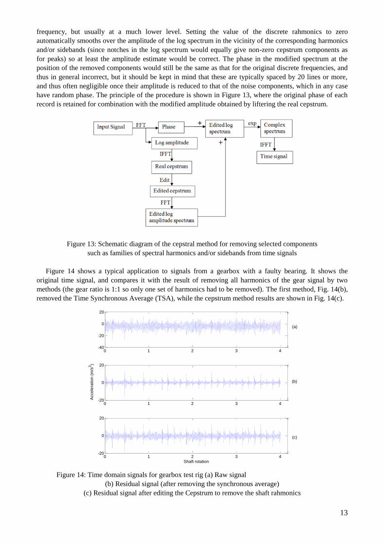
Figure 14 shows a typical application to signals from a gearbox with a faulty bearing. It shows the
original time signal, and compares it with the result of removing all harmonics of the gear signal by two
methods (the gear ratio is 1:1 so only one set of harmonics had to be removed). The first method, Fig. 14(b),
removed the Time Synchronous Average (TSA), while the cepstrum method results are shown in Fig. 14(c).
Figure 14: Time domain signals for gearbox test rig (a) Raw signal
(b) Residual signal (after removing the synchronous average)
(c) Residual signal after editing the Cepstrum to remove the shaft rahmonics
0 1 2 3 4-40
-20
0
20
0 1 2 3 4-20
0
20
0 1 2 3 4-20
0
20
Shaft rotation
Accele
ration (
m/s
2)
(a)
(b)
(c)
14
Even though the result of the cepstral method is slightly noisier than for the TSA, the subsequent
envelope analysis of the edited signals for the bearing diagnosis was just as successful.
Note that this cepstral method can also remove families of equally spaced sidebands, even where these are
not simultaneously harmonics, something which cannot be done by TSA.
5.1 Application to operational modal analysis
A frequent problem with operational modal analysis (OMA) is the presence of disturbing components in
the signal, for example discrete frequencies. These are often treated by the OMA software as modes with
very low damping. Families of harmonics and sidebands can be individually removed, as just described, but
another alternative that is often possible is to apply a lowpass lifter to the cepstrum to greatly enhance the
modal information with respect to everything else. By comparing equations (9) and (15) it is seen that both
contain damped exponentials, with the frequencies of the modes (and similar terms for the zeros), but the
cepstrum is additionally weighted by 1 n , making it shorter than the equivalent impulse response. Thus the
information about all modes is concentrated at low quefrency. Applying an exponential window (lowpass
lifter) to the cepstrum removes almost all extraneous information (including discrete frequencies) at higher
quefrencies, and the only effect on the modal information is to add a precisely known amount of extra
damping to each mode. This is the same in principle as using an exponential window in impact tests to cause
impulse responses to die out before the end of the record, but can in this case be applied to stationary signals,
rather than just transients starting at time zero.
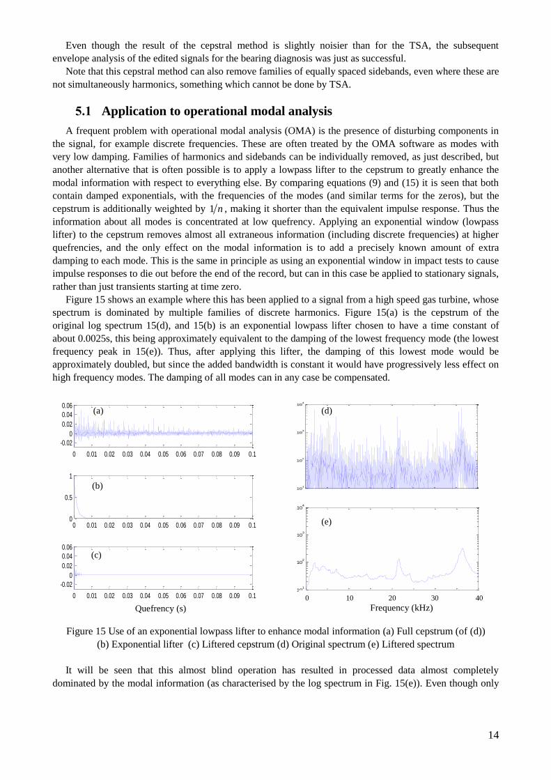
Figure 15 shows an example where this has been applied to a signal from a high speed gas turbine, whose
spectrum is dominated by multiple families of discrete harmonics. Figure 15(a) is the cepstrum of the
original log spectrum 15(d), and 15(b) is an exponential lowpass lifter chosen to have a time constant of
about 0.0025s, this being approximately equivalent to the damping of the lowest frequency mode (the lowest
frequency peak in 15(e)). Thus, after applying this lifter, the damping of this lowest mode would be
approximately doubled, but since the added bandwidth is constant it would have progressively less effect on
high frequency modes. The damping of all modes can in any case be compensated.
Figure 15 Use of an exponential lowpass lifter to enhance modal information (a) Full cepstrum (of (d))
(b) Exponential lifter (c) Liftered cepstrum (d) Original spectrum (e) Liftered spectrum
It will be seen that this almost blind operation has resulted in processed data almost completely
dominated by the modal information (as characterised by the log spectrum in Fig. 15(e)). Even though only
0 0.5 1 1.5 2 2.5 3 3.5 4
x 104
101
102
103
104
Frequency (Hz)
0 0.5 1 1.5 2 2.5 3 3.5 4
x 104
101
102
103
104
Frequency (Hz)
0 0.01 0.02 0.03 0.04 0.05 0.06 0.07 0.08 0.09 0.1
-0.02
0
0.02
0.04
0.06
0 0.01 0.02 0.03 0.04 0.05 0.06 0.07 0.08 0.09 0.10
0.5
1
0 0.01 0.02 0.03 0.04 0.05 0.06 0.07 0.08 0.09 0.1
-0.02
0
0.02
0.04
0.06
Time (s)Quefrency (s)
0 10 20 30 40
Frequency (kHz)
(a)
(b)
(c)
(d)
(e)

15
the spectrum is shown, time records are available which could be processed by standard OMA software.
Unfortunately, a modal analysis could not be carried out in this case as only one signal was available.
The same approach was however applied to the case of data from an in-flight helicopter, whose response
signals were contaminated by the harmonics of the rotor speed. In this case, the damping of the lowest mode
had a time constant of about 0.5s, which compared with 0.22s for the rotor period, so an exponential window
could not completely remove the first two rahmonics.
However, as shown in [31], the rotor harmonics could be largely removed, both by using a comb lifter
adjusted to the rahmonic spacing, and also with an exponential lifter on time constant 0.5s, but the best
results were obtained using a combination of both. These were comparable with the results of a method using
TSA to remove the rotor harmonics, but this was quite onerous because it required the signals first to be
order tracked to compensate for very small speed variations.
6 Conclusion
Few people realise that the cepstrum is older than the FFT algorithm, or that its original definition made it
less flexible as a result. Although originally applied to problems in seismology and speech analysis, similar
background situations meant that it was applied quite early to mechanical problems as well. There are two
main areas of applicability, which have been considerably developed over the years, one in detecting,
classifying and perhaps removing families of harmonics and sidebands in vibration and acoustic signals, and
the other in blind separation of source and transfer function effects, at least for SIMO systems. The latter
leads naturally to applications in operational modal analysis. Despite its long history, the author believes that
the cepstrum still has not been fully exploited, and it is hoped that this paper may stimulate further interest in
its possibilities.
Acknowledgments
The contributions of all my co-authors are gratefully acknowledged.
References
[1] B.P. Bogert, M.J.R. Healy, and J.W. Tukey, The Quefrency Alanysis of Time series for Echoes:
Cepstrum, Pseudo-Autocovariance, Cross-Cepstrum, and Saphe Cracking, in Proc. of the Symp. on
Time Series Analysis, by M. Rosenblatt (Ed.),. Wiley, NY, (1963), pp. 209-243.
[2] J.W. Cooley, J.W. Tukey, An Algorithm for the Machine Calculation of Complex Fourier Series, Math.
Of Comp., Vol. 19, No. 90, (1965), pp. 297-301.
[3] A.M. Noll, Cepstrum Pitch Determination, J.A.S.A, Vol. 41, No. 2, (1967), pp. 293-309.
[4] A.V. Oppenheim, R.W. Schafer, From Frequency to Quefrency: A History of the Cepstrum. IEEE
Signal Processing Magazine, September (2004), pp. 95-99, 106.
[5] A.V. Oppenheim, Superposition in a class of nonlinear systems, Ph.D. dissertation, MIT, May, (1964).
[6] R.W. Schafer, Echo removal by discrete generalized linear filtering, Ph.D. dissertation, MIT, Jan.
(1968).
[7] A.V. Oppenheim, R.W. Schafer, Digital Signal Processing, Englewood Cliffs, NJ: Prentice-Hall,
(1975).
[8] E.A. Robinson, Multi-channel Time Series Analysis with Digital Computer Programs. Holden-Day, San
Francisco (1967).
[9] R.B. Randall, Cepstrum Analysis and Gearbox Fault Diagnosis, Brüel and Kjær Application Note No.
13-150, Copenhagen (1973).
[10] R.B. Randall, Gearbox Fault Diagnosis using Cepstrum Analysis. Proc. IVth
World Congress on the
Theory of Machines and Mechanisms, Newcastle UK, IMechE, (1975) Vol.1 pp. 169-174.
16
[11] G. Sapy, Une Application du Traitement Numérique des Signaux au Diagnostic Vibratoire de Panne :
La Détection des Ruptures d’Aubes Mobiles de Turbines. Automatisme, Tome XX (1975), pp. 392-399.
[12] R.H. Lyon, A. Ordubadi, Use of Cepstra in Acoustic Signal Analysis, J.Mech.Design, Vol. 104, April
(1982), pp. 303-306.
[13] R.B. Randall, Separating Excitation and Structural Response Effects in Gearboxes. Third Int. Conf. on
Vib. in Rotating Machines, IMechE, York, (1984) pp. 101-107.
[14] R.B. Randall, Advanced Machine Diagnostics, The Shock and Vibration Digest, Willowbrook, IL,
USA, Vibration Institute, Vol. 29, No. 1 (1997) pp. 6-30.
[15] R.B. Randall, Cepstrum Analysis and Gearbox Fault Diagnosis, Maintenance Management
International, Elsevier (1982/1983) pp. 183-208.
[16] R.B. Randall, Vibration-based Condition Monitoring: Industrial, Aerospace and Automotive
Applications, Wiley (Chichester, UK) January (2011).
[17] C. Capdessus, M. Sidahmed, Analyse des vibrations d'un engrenage : cepstre, corrélation, spectre.
Traitement du Signal, Vol. 8, No. 5 (1991), pp. 365-372.
[18] M. El Badaoui, F. Guillet, J. Danière, Contribution du Cepstre d’Énergie au Diagnostic de Réducteur
Complexe à Engrenage, Revue Française de Mécanique, RFM, No. 1999-1, (1991) pp. 4-7.
[19] M. El Badaoui, J. Antoni, F. Guillet, J. Danière, P. Velex, Use of the moving cepstrum integral to detect
and localise tooth spalls in gears, Mechanical Systems and Signal Processing, September 2001, pp.
[20] El Badaoui, F. Guillet, J. Danière, New applications of the real cepstrum to gear signals, including
definition of a robust fault indicator, Mechanical Systems and Signal Processing, Vol. 18, No. 5,
September (2004), pp. 1031-1046.
[21] H. Endo, R.B. Randall, C. Gosselin, Differential diagnosis of spalls vs. cracks in the gear tooth fillet
region, Journal of Failure Analysis and Prevention Vol. 4 No. 5, (2004) pp. 57-65.
[22] R.B. Randall, Cepstral Methods of Operational Modal Analysis. Chapter 24 in Encyclopedia of
Structural Health Monitoring, Wiley (2009).
[23] A. Polydoros, A.T. Fam, The Differential Cepstrum: Definitions and Properties, Proc. IEEE Int. Symp.
Circuits Systems, (1981) pp. 77-80.
[24] Y. Gao, R.B. Randall, Determination of Frequency Response Functions from Response Measurements.
Part I: Extraction of Poles and Zeros from Response Cepstra, Mechanical Systems and Signal
Processing, Vol. 10 No. 3 (1996) pp. 293-317.
[25] Y. Gao, R.B. Randall, Determination of Frequency Response Functions from Response Measurements.
Part II: Regeneration of Frequency Response Functions from Poles and Zeros, Mechanical Systems and
Signal Processing, Vol. 10 No. 3 (1996), 319-340.
[26] R.B. Randall, W.A. Smith, Cepstrum-based operational modal analysis: regeneration of frequency
response functions, ACAM7, Engineers Australia, Adelaide, December, (2012).
[27] J. Antoni, F. Guillet, J. Danière, Identification of Non-Minimum Phase Transfer Functions From
Output-Only Measurements, ISMA25 Conference, KUL, Leuven Belgium, (2000).
[28] J. Antoni, S. Braun (Eds.) Special Issue: Blind Source Separation. Mechanical Systems and Signal
Processing, Vol. 19, No. 6, November (2005).
[29] D. Hanson, R.B. Randall, J. Antoni, D.J. Thompson, T.P. Waters, R.A.J. Ford, Cyclostationarity and the
cepstrum for operational modal analysis of mimo systems—Part I: Modal parameter identification,
Mechanical Systems and Signal Processing, Vol. 21 No. 6 (2007) pp. 2441-2458.
[30] N. Sawalhi, R.B. Randall, Editing Time Signals using the Real Cepstrum. MFPT conference, Virginia
Beach, May (2011).
[31] R.B. Randall, B. Peeters, J. Antoni, S. Manzato, New cepstral methods of signal pre-processing for
operational modal analysis, ISMA2012, Leuven, Belgium, September (2012) pp. 755-764.