a hierarchical voxel hash for fast 3d nearest neighbor lookup

A Hierarchical Voxel Hash for Fast 3D NearestNeighbor Lookup

Bertram Drost1 and Slobodan Ilic2

1MVTec Software GmbH, 2Technische Universitat Munchen

Abstract. We propose a data structure for finding the exact nearestneighbors in 3D in approximately O(log(log(N)) time. In contrast tostandard approaches such as k-d-trees, the query time is independentof the location of the query point and the distribution of the data set.The method uses a hierarchical voxel approximation of the data point’sVoronoi cells. This avoids backtracking during the query phase, whichis a typical action for tree-based methods such as k-d-trees. In addition,voxels are stored in a hash table and a bisection on the voxel level is usedto find the leaf voxel containing the query point. This is asymptoticallyfaster than letting the query point fall down the tree. The experimentsshow the method’s high performance compared to state-of-the-art ap-proaches even for large point sets, independent of data and query setdistributions, and illustrates its advantage in real-world applications.

1 Introduction

Quickly finding the closest point from a large set of data points in 3D is cru-cial for alignment algorithms, such as ICP, as well as industrial inspection androbotic navigation tasks. Most state-of-the-art methods for solving the nearestneighbor problem in 3D are based on recursive subdivisions of the underlyingspace to form a tree of volumes. The various subdivision strategies include uni-form subdivisions, such as octrees [14], as well as non-uniform subdivisions, suchas k-d-trees [2] and Delaunay or Voronoi based subdivisions.

Tree-based methods require two steps to find the exact nearest neighbor.First, the query point falls down the tree to find its corresponding leaf node. Sincethe query point might be closer to the boundary of the node’s volume than to thedata points contained in the leaf node, tree backtracking is required as a secondstep to search neighboring volumes for the closest data point. The proposedmethod improves the time for finding the leaf node and removes the need forpotentially expensive backtracking by using voxels to recursively subdivide space.The leaf voxel that contains the query point is found by bisecting the voxel size.For trees of depth L, this approach requires only O(log(L)) operations, insteadof O(L) operations when letting the query point fall down the tree. In addition,each voxel contains a list of all data points whose Voronoi cells intersect thatvoxel, such that no backtracking is necessary. By storing the voxels in a hash tableand enforcing a limit on the number of Voronoi intersections per voxel, the totalquery time is independent of the position of the query point and the distribution

2 Bertram Drost and Slobodan Ilic

of data points. The theoretical query time is of magnitude O(log(log(N)), whereN is the size of the target data point set.

The amount of backtracking that is required in tree-based methods dependson the position of the query point. Methods based on backtracking thereforehave non-constant query times even when using the same dataset, making themdifficult to use in real-time applications. Since the proposed method does notrequire backtracking, the query time becomes almost independent of the positionof the query point. Further, the method is largely parameter free, does not requirean a-priori definition of a maximum query range, and is straightforward and easyto implement.

We evaluate the proposed method on different synthetic datasets that showdifferent distributions of the data and query point sets, and compare it to twostate of the art methods: a self-implemented k-d-tree and the Approximate Near-est Neighbour (ANN) library [15], which, contrary to its name, allows also tosearch for exact nearest neighbors. The experiments show that the proposedmethod is significantly faster for larger data sets and shows an improved asymp-totic behaviour. As a trade-off, the proposed method uses a more expensivepreprocessing step. Finally, we demonstrate the performance of the proposedmethod within two applications on real-world datasets, pose refinement and sur-face inspection. The runtime of both applications is dominated by the nearestneighbor lookups, which is why both greatly benefit from the proposed method.

2 Related Work

An extensive overview over different nearest neighbor search strategies can befound in [17]. Nearest-neighbor search strategies can roughly be divided into tree-based and hash-based approaches. Concerning tree-based methods, variants ofthe k-d-tree [2] are state-of-the-art for applications such as ICP, navigation andsurface inspection [8]. For high-dimensional datasets, such as images or iamgedescriptors, embeddings into lower-dimensional spaces are sometimes used toreduce the complexity of the problem [13].

Many methods were proposed for improving the nearest neighbor query timeby allowing small errors in the computed closest point, i.e., by solving the ap-proximate nearest neighbor problem [1, 11, 6]. While faster, using approximationschanges the nature of the lookup and is only applicable for methods such as ICP,where a small number of incorrect correspondences can be dealt with statisti-cally. The iterative nature of ICP can be used to accelerate subsequent nearestneighbor lookups through caching [16, 10]. Such approaches are, however, onlyusable for ICP and not for defect detection or other tasks.

Yan and Bowyer [18] proposed a regular 3D grid of voxels that allow constant-time lookup for a closest point, by storing a single closest point per voxel. How-ever, such fixed-size voxel grids use excessive amounts of memory and require atradeoff between memory consumption and lookup speed. The proposed multi-level adaptive voxel grid overcomes this problem, since more and smaller voxelsare created only at the ‘interesting’ parts of the data point cloud, while thespeed advantage of hashing is mostly preserved. Glassner [9] proposed to use ahash-table for accessing octrees, which is the basis for the proposed approach.

A Hierarchical Voxel Hash for Fast 3D Nearest Neighbor Lookup 3

Using Voronoi cells is a natural way to approach the nearest neighbor prob-lem, since a query point is always contained in the Voronoi cell of its nearestneighbor. Boada et al . [5] proposed an octree that approximates generalizedVoronoi cells and that can be used to approximately solve the nearest neighborproblem [4]. Their work also gives insight into the construction costs of suchan octree. Contrary to the proposed work, their work concentrates on the con-struction of the data structure and solves the nearest neighbor problem onlyapproximately. Additionally, their proposed octree still requires O(depth) oper-ations for a query. However, their work indicates how the proposed method canbe generalized to other metrics and to shapes other than points. Similar, [12]proposed an octree-like approximation of the Voronoi tesselation. Birn et al . [3]proposed a full hierarchy of Delaunay triangulations for 2D nearest neighborlookups. However, the authors state that their approach is unlikely to work wellin 3D and beyond.

3 Method

Notation and Overview We denote points from the original data set as x ∈ Dand points of the query set q ∈ Q. Given a query point q, the objective is tofind the closest point NN(q, D) = argminx∈D |q − x|2. The individual Voronoicells of the Voronoi diagram of D are denoted voro(x), which we see as closedset.

The proposed method requires a pre-processing step where the voxel hashstructure for the data set D is created. Once this data structure is precomputed,it remains unchanged and can be used for subsequent queries. The creation ofthe data structure is done in three steps: The computation of the Voronoi cellsfor the data set D, the creation of the octree and the transformation of the octreeinto a hash table.Octree Creation Using Voronoi cells is a natural way to approach the nearestneighbor problem. A query point q is always contained within the Voronoi cellof its closest point, i.e., q ∈ voro(NN(q, D)). Thus, finding a Voronoi cell thatcontains q is equivalent to finding NN(q, D). However, the irregular and data-dependent structure of the Voronoi tessellation does not allow a direct lookup.We thus use the octree to create a more regular structure on top of the Voronoidiagram, which allows to quickly find the corresponding Voronoi cell.

After computing the Voronoi cells for the data set D, an octree is created,whose root voxel contains the expected query range. Note that the root voxelcan be several thousand times larger than the extend of the data set withoutsignificant performance implications.

Contrary to traditional octrees, where voxels are split based on the numberof contained data points, we split each voxel based on the number of intersectingVoronoi cells: Each voxel that intersects more than Mmax Voronoi cells is splitinto eight sub-voxels, which are processed recursively. Fig. 1 shows a 2D examplefor this splitting. The set of data points whose Voronoi cells intersect a voxel vis denoted

L(D, v) = {x ∈ D : voro(x) ∩ v 6= ∅}. (1)


Fig. 1. Toy example in 2D of the creation of the hierarchical voxel structure. For thedata point set (left), the Voronoi cells are computed (center). Starting with the rootvoxel that encloses all points, voxels are recursively split if the number of intersectingVoronoi cells exceeds Mmax. In this example, the root voxel is split until each voxelintersects at most Mmax = 5 Voronoi cells (right).

This splitting criterion allows a constant processing time during the query phase:For any query point q contained in a leaf voxel vleaf , the Voronoi cell of theclosest point NN(q, D) must intersect vleaf . Therefore, once the leaf node voxelthat contains q is found, at most Mmax data points must be searched for theclosest point. The given splitting criterion thus removes the requirement forbacktracking.

The cost for this is a deeper tree, since a voxel typically intersects moreVoronoi cells than it contains data points. The irregularity of the Voronoi tes-sellation and possible degenerated cases, as discussed below, make it difficult togive theoretical bounds on the depth of the octree. However, experimental vali-dation shows that the number of created voxels scales linearly with the numberof data points |D| (see Fig. 4(a)).

Hash Table The result of the recursive subdivision is an octree, as depictedin Fig. 1. To find the closest point of a given query point q, two steps arerequired: Find the leaf voxel vleaf (q) which contains q and search all points inL(D, vleaf (q)) for the closest point of q. The computation costs for finding theleaf node are on average O(depth) ≈ O(log(|D|)) when letting q fall down thetree. We propose to use the regularity of the octree to reduce those costs toO(log(depth)) ≈ O(log(log(|D|))). For this, all voxels of the octree are stored ina hash table which is indexed by the voxel’s level l(v) and its index idx(v) ∈ Zd


Level

1

2

3

4

5

6

7

8

9

Hash Table

(l = 9, idx1)

(l = 5, idx2)

(l = 3, idx3)

∅

(a)

l1 = 5

l3 = 6

l2 = 7

(b)

Fig. 2. (a) The hash table stores all voxels v, which are indexed through their levell and their index idx. The hash table allows to check for the existence of a voxel inconstant time. (b) Toy example in 2D of how to find the leaf voxel by bisecting itslevel. Finding the leaf node by letting the query point fall down the tree would requireO(depth) operations on average (green path). Instead, the leaf node is found throughbisection of its level. In each step, the hash table is used to check for the presence ofthe corresponding voxel. The search starts with the center level l1 and, since the voxelexists, proceeds with l2. Since the voxel at level l2 does not exist, level l3 is checkedand the leaf node is found.

(Fig. 2(a)). idx(v) is the integer-valued position of the voxel within the voxelgrid of its level l(v).

The leaf voxel vleaf (q) is then found through bisection of its level. The min-imum and maximum voxel level is initialized as lmin = 1 and lmax = depth.The existence of the voxel with the ‘center’ level lc = b(lmin + lmax)/2c is testedusing the hash table. If the voxel exists, the search proceeds with the interval[lc, lmax]. Otherwise, it proceeds to search the interval [lmin, lc − 1]. The searchcontinues until the interval contains only one level, which is the level of the leafvoxel vleaf (q). Fig. 2 illustrates this bisection on a toy example.

Note that in our experiments, tree depths were in the order of 20-40 such thatthe expected speedup over the traditional method was around 5. Additionally,each voxel in the hash table contains the minimum and maximum depth of itssubtree to speedup the bisection. Additionally, the lists L(D, v) are stored onlyfor the leaf nodes. The primary cost during the bisection are cache misses whenaccessing the hash table. Therefore, an inlined hash table is used to reduce theaverage amount of cache misses.

Degenerated Cases For some degenerated cases, the proposed method forsplitting voxels based on the number of intersecting Voronoi cells might notterminate. This happens when more than Mmax Voronoi cells meet at a singlepoint, as depicted in Fig. 3. To avoid infinite recursion, a limit Lmax on the depthof the octree is enforced. In such cases, the query time for points that fall withinsuch an unsplit leaf voxel is larger than for other query points. However, we


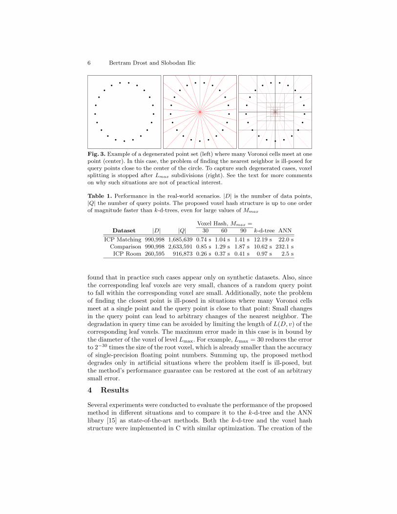
Fig. 3. Example of a degenerated point set (left) where many Voronoi cells meet at onepoint (center). In this case, the problem of finding the nearest neighbor is ill-posed forquery points close to the center of the circle. To capture such degenerated cases, voxelsplitting is stopped after Lmax subdivisions (right). See the text for more commentson why such situations are not of practical interest.

Table 1. Performance in the real-world scenarios. |D| is the number of data points,|Q| the number of query points. The proposed voxel hash structure is up to one orderof magnitude faster than k-d-trees, even for large values of Mmax

Voxel Hash, Mmax =Dataset |D| |Q| 30 60 90 k-d-tree ANN

ICP Matching 990,998 1,685,639 0.74 s 1.04 s 1.41 s 12.19 s 22.0 sComparison 990,998 2,633,591 0.85 s 1.29 s 1.87 s 10.62 s 232.1 sICP Room 260,595 916,873 0.26 s 0.37 s 0.41 s 0.97 s 2.5 s

found that in practice such cases appear only on synthetic datasets. Also, sincethe corresponding leaf voxels are very small, chances of a random query pointto fall within the corresponding voxel are small. Additionally, note the problemof finding the closest point is ill-posed in situations where many Voronoi cellsmeet at a single point and the query point is close to that point: Small changesin the query point can lead to arbitrary changes of the nearest neighbor. Thedegradation in query time can be avoided by limiting the length of L(D, v) of thecorresponding leaf voxels. The maximum error made in this case is in bound bythe diameter of the voxel of level Lmax. For example, Lmax = 30 reduces the errorto 2−30 times the size of the root voxel, which is already smaller than the accuracyof single-precision floating point numbers. Summing up, the proposed methoddegrades only in artificial situations where the problem itself is ill-posed, butthe method’s performance guarantee can be restored at the cost of an arbitrarysmall error.

4 Results

Several experiments were conducted to evaluate the performance of the proposedmethod in different situations and to compare it to the k-d-tree and the ANNlibary [15] as state-of-the-art methods. Both the k-d-tree and the voxel hashstructure were implemented in C with similar optimization. The creation of the


100

101

102

103

104

105

106

107

102 103 104 105 106

NumberofVoxels

Number of Points

Mmax = 30Mmax = 60Mmax = 90

(a)

10−5

10−4

10−3

10−2

10−1

100

101

102

103

102 103 104 105 106

Creation

Tim

eins

Number of Points


Voronoi CellsKD-Tree

ANN

(b)

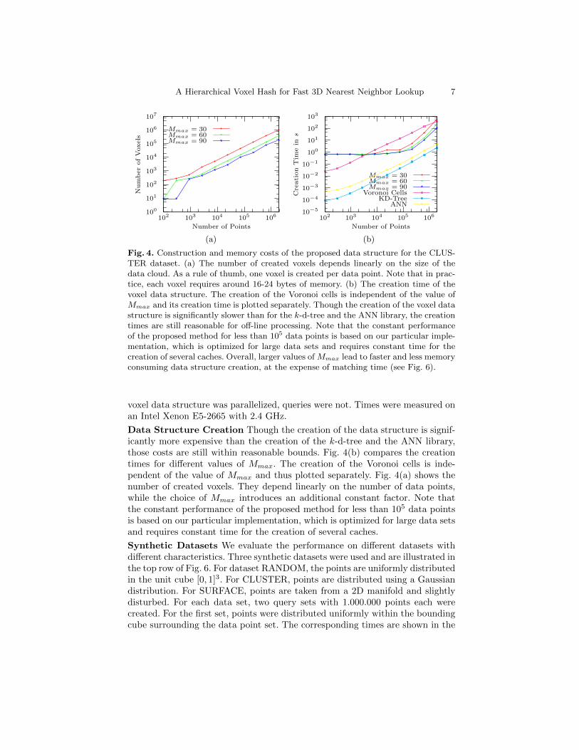
Fig. 4. Construction and memory costs of the proposed data structure for the CLUS-TER dataset. (a) The number of created voxels depends linearly on the size of thedata cloud. As a rule of thumb, one voxel is created per data point. Note that in prac-tice, each voxel requires around 16-24 bytes of memory. (b) The creation time of thevoxel data structure. The creation of the Voronoi cells is independent of the value ofMmax and its creation time is plotted separately. Though the creation of the voxel datastructure is significantly slower than for the k-d-tree and the ANN library, the creationtimes are still reasonable for off-line processing. Note that the constant performanceof the proposed method for less than 105 data points is based on our particular imple-mentation, which is optimized for large data sets and requires constant time for thecreation of several caches. Overall, larger values of Mmax lead to faster and less memoryconsuming data structure creation, at the expense of matching time (see Fig. 6).

voxel data structure was parallelized, queries were not. Times were measured onan Intel Xenon E5-2665 with 2.4 GHz.

Data Structure Creation Though the creation of the data structure is signif-icantly more expensive than the creation of the k-d-tree and the ANN library,those costs are still within reasonable bounds. Fig. 4(b) compares the creationtimes for different values of Mmax. The creation of the Voronoi cells is inde-pendent of the value of Mmax and thus plotted separately. Fig. 4(a) shows thenumber of created voxels. They depend linearly on the number of data points,while the choice of Mmax introduces an additional constant factor. Note thatthe constant performance of the proposed method for less than 105 data pointsis based on our particular implementation, which is optimized for large data setsand requires constant time for the creation of several caches.

Synthetic Datasets We evaluate the performance on different datasets withdifferent characteristics. Three synthetic datasets were used and are illustrated inthe top row of Fig. 6. For dataset RANDOM, the points are uniformly distributedin the unit cube [0, 1]3. For CLUSTER, points are distributed using a Gaussiandistribution. For SURFACE, points are taken from a 2D manifold and slightlydisturbed. For each data set, two query sets with 1.000.000 points each werecreated. For the first set, points were distributed uniformly within the boundingcube surrounding the data point set. The corresponding times are shown in the


(a) (b)

Fig. 5. Example application for the proposed method. A 3D scan of the scene wasacquired using a multi-camera stereo setup and approximate poses of the pipe joint werefound using the method of Drost et al . [7]. (a) The poses were refined using ICP. Thecorresponding nearest neighbor lookups were logged and used for the evaluation showin Table 1. (b) For each scene point close to one of the detected objects, the distanceto the object is computed and visualized. This allows the detection of defects on thesurface of the objects. The lookups were again logged and used for the performanceevaluation in Table 1.

center row of Fig. 6. The second query set has the same distribution as the dataset, with the corresponding timings shown in the bottom row of Fig. 6.

The proposed data structure is significantly faster than the simple k-d-treefor all datasets with more than 105 points. The ANN library shows similarperformance than the proposed method for Mmax = 30 for the RANDOM andCLUSTER datasets. For the SURFACE dataset, our method clearly outperformsANN even for smaller point clouds. Note that the SURFACE dataset representsa 2D manifold and thus shows the behaviour for ICP and other surface-basedapplications. Overall, the performance of the proposed method is less dependenton the distribution of data and query points. This advantage allows our methodto be used in real-time environments.

Real-World Datasets Finally, real-world examples were used for evaluating theproposed method’s performance. First, several instances of an industrial objectwere detected in a scene acquired with a multi-camera stereo setup. The originalscene and the matches are shown in Fig. 5. We found approximate positionsof the target object using the method of Drost et al . [7] and subsequently usedICP for each match for a precise alignment. The nearest neighbor lookups duringICP were logged and later evaluated with the available methods. The sizes ofthe data clouds and the lookup times are shown in Table 1.

Afterwards, we used the proposed method to find surface defects of the de-tected objects. For this, the distances of the scene points to the closest foundmodel were computed. The distances are visualized in Fig. 5(b) and show a sys-tematic error in the modeling of the object. We are, however, only interested inthe required inspection time, which is shown in Table 1.

Finally, we used a Kinect sensor to acquire two slightly rotated scans ofan office room and aligned both scans using ICP. For all three datasets, the


proposed method significantly outperforms both our k-d-tree implementationand the ANN library by up to one order of magnitude.

5 Conclusion

We proposed and evaluated a novel data structure for nearest-neighbor lookupin 3D, which can easily be extended to 2D. Compared to traditional tree-basedmethods, backtracking was made redundant by building an octree on top of theVoronoi diagram. In addition, a hash table was used, allowing a fast bisectionsearch of the leaf voxel of a query point, which is faster than letting the querypoint fall down the tree. The proposed method combines the best of tree-basedapproaches and fixed voxel grids.

The evaluation on synthetic datasets shows that the proposed method isfaster than traditional k-d-trees and the ANN library on larger datasets and has aquery time which is almost independent of the data and query point distribution.Though the proposed structure takes significantly longer to be created, thosetimes are still within reasonable bounds. The evaluation on real datasets showsthat real-world scenarios such as ICP and surface defect detection greatly benefitfrom the performance of the method.

References

1. Arya, S., Mount, D.M., Netanyahu, N.S., Silverman, R., Wu, A.Y.: An optimalalgorithm for approximate nearest neighbor searching fixed dimensions. JACM45(6), 891–923 (1998)

2. Bentley, J.L.: Multidimensional binary search trees used for associative searching.Communications of the ACM 18(9), 509–517 (1975)

3. Birn, M., Holtgrewe, M., Sanders, P., Singler, J.: Simple and fast nearest neighborsearch. In: 11th Workshop on Algorithm Engineering and Experiments (2010)

4. Boada, I., Coll, N., Madern, N., Sellares, J.A.: Approximations of 3D generalizedvoronoi diagrams. 21th Europ. Workshop on Comp. Geometry (2005)

5. Boada, I., Coll, N., Madern, N., Sellares, J.A.: Approximations of 2D and 3Dgeneralized voronoi diagrams. Int. Journal of Computer Mathematics 85(7) (2008)

6. Choi, W.S., Oh, S.Y.: Fast nearest neighbor search using approximate cached kdtree. In: IROS (2012)

7. Drost, B., Ulrich, M., Navab, N., Ilic, S.: Model globally, match locally: Efficientand robust 3D object recognition. In: CVPR (2010)

8. Elseberg, J., Magnenat, S., Siegwart, R., Nuechter, A.: Comparison of nearest-neighbor-search strategies and implementations for efficient shape registration.Journal of Software Engineering for Robotics 3(1), 2–12 (Mar 2012)

9. Glassner, A.S.: Space subdivision for fast ray tracing. Computer Graphics andApplications, IEEE 4(10), 15–24 (1984)

10. Greenspan, M., Godin, G.: A nearest neighbor method for efficient ICP. In: 3-DDigital Imaging and Modeling. IEEE (2001)

11. Greenspan, M., Yurick, M.: Approximate kd tree search for efficient ICP. In: 3DIM2003. IEEE (2003)

12. Har-Peled, S.: A replacement for voronoi diagrams of near linear size. In: Proc. onFoundations of Computer Science. pp. 94–103 (2001)

13. Hwang, Y., Han, B., Ahn, H.K.: A fast nearest neighbor search algorithm by non-linear embedding. In: CVPR (2012)


0

2

4

6

8

10

102 103 104 105 106

RANDOM

DIS

TRIB

UTIO

N

Tim

eperquery

point[µ

s]

Number of Points


KD-TreeANN

0

2

4

6

8

10

102 103 104 105 106

Number of Points

0

2

4

6

8

10

102 103 104 105 106

Number of Points

0

2

4

6

8

10

102 103 104 105 106SAM

EDIS

TRIB

UTIO

N

Tim

eperquery

point[µ

s]

Number of Points

0

2

4

6

8

10

102 103 104 105 106

Number of Points

0

2

4

6

8

10

102 103 104 105 106

Number of Points

Fig. 6. Query time per query point for different synthetic datasets and methods. Eachcolumn represents a different dataset. From left to right: RANDOM, CLUSTER, andSURFACE dataset. The x-axis shows the number of data points, i.e., |D|, the y-axisshows the average query time per query point. For the center row, query points werewere randomly selected from the cuboid surrounding the data. For the bottom row,query points were taken from the same distribution as the data points. The querytime for the proposed method is less dependent of the number of data points andalmost independent of the distribution of the data and query points. It is especially ofadvantage for very large datasets, as well as for datasets representing 2D manifolds.

14. Meagher, D.: Geometric modeling using octree encoding. Computer graphics andimage processing 19(2), 129–147 (1982)

15. Mount, D.M., Arya, S.: ANN: A library for approximate nearest neighbor search-ing, http://www.cs.umd.edu/˜mount/ANN/

16. Nuchter, A., Lingemann, K., Hertzberg, J.: Cached kd tree search for ICP algo-rithms. In: 3DIM 2007. IEEE (2007)

17. Samet, H.: Foundations of Multidimensional And Metric Data Structures. MorganKaufmann (2006)

18. Yan, P., Bowyer, K.W.: A fast algorithm for ICP-based 3D shape biometrics. Com-puter Vision and Image Understanding 107(3) (2007)

a hierarchical voxel hash for fast 3d nearest neighbor lookup

Documents